Supplementary Material: Predicting the Electronic Density Response of Condensed-Phase Systems to Electric Field Perturbations

I Machine learning parameters for bulk water and naphthalene

In bulk water, there are physical atoms distributed throughout each spherical atomic environment $A_{i}$. As such, it is not clear a priori where the dummy atom should be placed within this environment, or what the optimal width of the associated Gaussian should be. To determine these values ($x$ and $\zeta$ in Eq. (LABEL:eq:environment2) in the main text), we took a subset of 50 structures from the full training set, selected 40 of those to form a training set and used the remainder as the test set, and calculated the % RMSE error as a function of $x$ and $\zeta$, using $M=200$. Our results are shown in Fig. 1; we found that the error decreased monotonically with increasing $\zeta$ at all values of $x$, approaching an asymptote at large values, while for large values of $\zeta$ we found a broad minimum in $x$ centred at around 0.3. Therefore, $x=0.3$ and $\zeta=1.0$ Å define the dummy atom in our calculations. Since we did not observe a deep minimum in these results, we felt confident using the same parameters for naphthalene without repeating this optimisation procedure.

The learning curves for the density response to a field applied along the $x$ axis are shown in Fig. 2, using the full dataset. As can be seen, learning improves monotonically with increasing training set size, with the error reaching a plateau for $N\geq 100$. The value of this plateau is reduced as the number of reference environments is increased, converging at $M=3000$ with errors just below 12%. The equivalent learning curves for naphthalene are shown in Fig. 3, showing similar behaviour, with errors converging for $M=2000$ at around 6%.

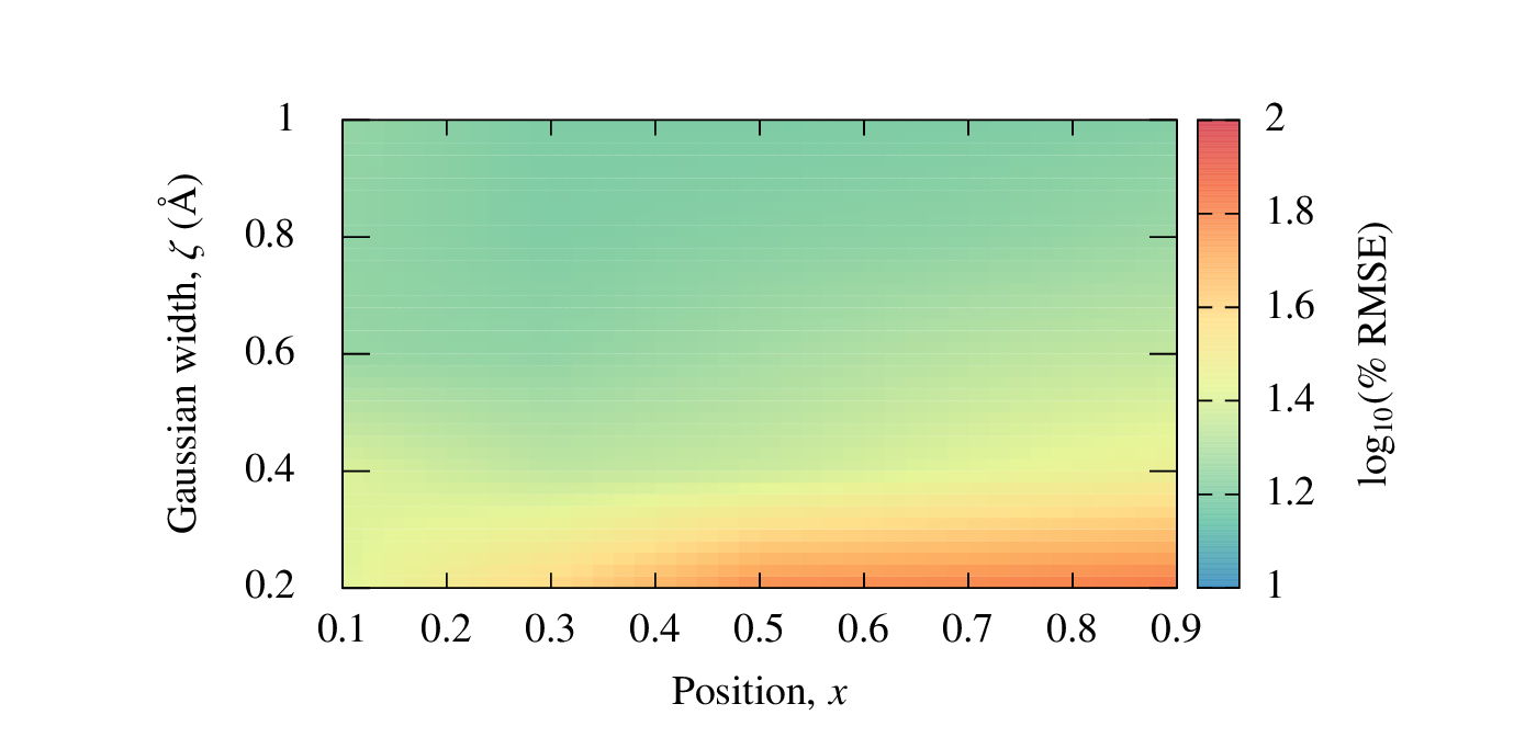
Figure 1: The % RMSE in the density response to a field applied along the $x$ axis for a test set of 10 water configurations, as a function of the parameters $x$ and $\zeta$ which define the position and Gaussian width associated with the dummy atom added to the atomic environment. In all cases the machine learning model is trained with $N=40$, $M=200$.

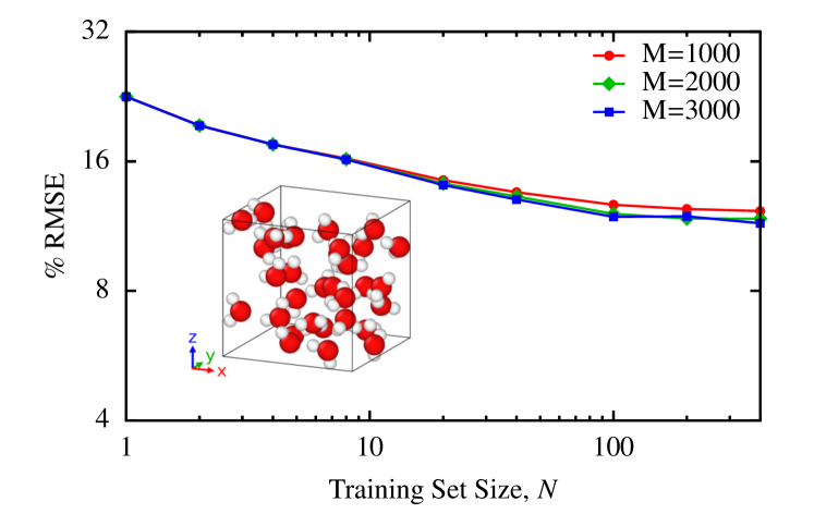
Figure 2: Learning curves for the predicted density response to an applied field along the $x$ axis for the full bulk water dataset, converging with respect to $M$.

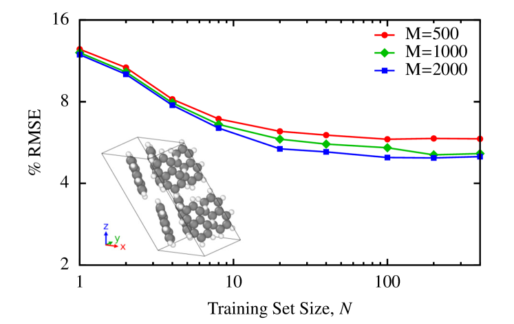
Figure 3: Learning curves for the predicted density response to an applied field along the $x$ axis for the naphthalene dataset, converging with respect to $M$.

II Explaining the errors in the dielectric susceptibility of naphthalene

As noted in the main text, we observe a counter-intuitive relationship between the error in the predicted density response of naphthalene and the error in the dielectric susceptibility derived from that predicted response. Specifically, we observe the lowest errors in the predicted response to a field applied along the $z$ axis, but the largest errors in the dielectric susceptibility tensor for the components derived from this response; the reverse is true for the predicted response to a field applied along the $x$ axis. This apparent paradox can be explained in general terms by noting that the errors in properties derived from the predicted density response depend on the distribution of the error of the density response, as well as its overall magnitude. We noted this phenomenon in our previous work predicting the electron density – in that case we found that errors in the electrostatic energy derived from the predicted density were particularly sensitive to errors in the electron density located close to the nuclei.Grisafi et al. (2022)

The errors in the predicted density response to a field applied along the $x$ and $z$ axes of a representative naphthalene configuration are shown in Figure 4. In both cases the error in the density is localised primarily on the surfaces of the molecule normal to the applied field, with a region of positive error on one surface and of negative error on the opposing surface. Since the surface area of the molecule is largest normal to the $x$ axis, we observe a larger overall error in the density response when the field is applied along the $x$ axis than when it is applied along the $z$ axis. However, from Eq. (LABEL:eq:alpha) in the main text it can be shown that for a given magnitude of error in the density response, the magnitude of the corresponding error in the polarizability is determined by the separation between the regions of positive and negative error in the density response. To illustrate this, we imagine a simple description of an error in the density response:

$$\tilde{\rho}^{(1)}_{\beta}(\bm{r})=\rho^{(1)}_{\beta}(\bm{r})+\varepsilon\delta(\bm{r}^{\prime})-\varepsilon\delta(\bm{r}^{\prime\prime}).$$ (1)

Here $\tilde{\rho}^{(1)}_{\beta}(\bm{r})$ is an approximate density response, $\rho^{(1)}_{\beta}(\bm{r})$ is the exact density response, $\varepsilon$ is the magnitude of the error found at two points in space $\bm{r}^{\prime}$ and $\bm{r}^{\prime\prime}$, and $\delta(\bm{r})$ is the Dirac delta function. There are two error terms of equal and opposite magnitude since the approximate density response must integrate to zero. The error in the polarizability arising from this error is given by

$$\begin{split}\tilde{\alpha}_{\gamma\beta}-\alpha_{\gamma\beta}=&-\int_{\textrm{u.c.}}r_{\gamma}\left(\tilde{\rho}^{(1)}_{\beta}(\bm{r})-\rho^{(1)}_{\beta}(\bm{r})\right)\textrm{d}\bm{r}\\ &=\int_{\textrm{u.c.}}r_{\gamma}\left(\varepsilon\delta(\bm{r}^{\prime})-\varepsilon\delta(\bm{r}^{\prime\prime})\right)\textrm{d}\bm{r}\\ &=\varepsilon\left(r^{\prime}_{\gamma}-r^{\prime\prime}_{\gamma}\right).\end{split}$$ (2)

Therefore, for a fixed value of the error $\varepsilon$, then the greater the spatial separation in the $\gamma$ direction between these regions of error, the larger the error in the polarizability and dielectric susceptibility. Since the long axis of naphthalene lies approximately along close to the $z$ axis, the separation between these regions is largest when a field is applied along the $z$ axis, and we therefore see much larger errors in the corresponding components of the dielectric susceptibility, despite the fact that the actual magnitude of the error in the density response is lowest for this field direction.

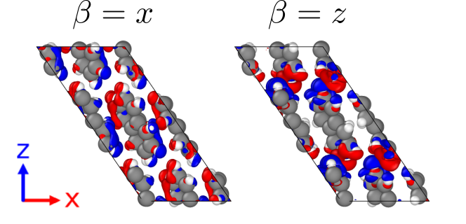
Figure 4: Isosurfaces at $\pm$ 0.01 VÅ^-2 of the error in the predicted density response to a field applied along the $x$ axis (left) and $z$ axis (right) for a particular configuration of naphthalene. Positive errors are shown in blue, negative errors in red.

References

- Grisafi et al. (2022) A. Grisafi, A. M. Lewis, M. Rossi, and M. Ceriotti, Journal of Chemical Theory and Computation (2022), 10.1021/ACS.JCTC.2C00850, arxiv:2206.14087 .