Stable intermediate phase of secondary structures for semiflexible polymers

Abstract

Systematic microcanonical inflection-point analysis of precise numerical results obtained in extensive generalized-ensemble Monte Carlo simulations reveals a bifurcation of the coil-globule transition line for polymers with a bending stiffness exceeding a threshold value. The region, enclosed by the toroidal and random-coil phases, is dominated by structures crossing over from hairpins to loops upon lowering the energy. Conventional canonical statistical analysis is not sufficiently sensitive to allow for the identification of these separate phases.

For more than a century, canonical statistical analysis has been the standard procedure for the quantitative description of thermodynamic phase transitions in systems large enough to allow for making use of the thermodynamic limit in analytic calculations and finite-size scaling methods in computational approaches. However, throughout the last few decades, interest has increasingly shifted toward understanding the thermal transition behavior of systems at smaller scales, including, but not limited to, biomolecular systems such as proteins, DNA and RNA.

The impact of finite-size and surface effects on the formation of structural phases and the transitions that separate them is so significant that conventional statistical analysis methods are not sensitive enough to provide a clear picture of the system behavior. Recently developed approaches like the generalized microcanonical inflection-point analysis method [1] overcome this issue as they allow for a systematic and unambiguous identification and classification of transitions in systems of any size.

One particularly intriguing problem is the characterization of phases for entire classes of semiflexible polymers, which, for example, include variants of DNA and RNA. This has been a long-standing problem, but simple early approaches such as the wormlike-chain or Kratky-Porod model [2] could not address this problem. Significant advances in the development of Monte Carlo algorithms and vastly improved technologies enabled the computer simulation of more complex coarse-grained models in recent years, though [3, 4, 5, 6, 7]. Yet, most of these studies still employed conventional canonical statistical analysis techniques that led to a plethora of results. This is partly due to the fact that canonical statistical analysis, which is usually based on locating extremal points in thermodynamic response functions such as the specific heat and temperature derivatives of order parameters or in free-energy landscapes, is ambiguous, inconsequential, and often not sufficiently sensitive to allow for the systematic construction of a phase diagram for finite systems.

In this Letter, we take a closer look at the most interesting part of the hyperphase diagram of the generic model for semiflexible polymers in the space of bending stiffness and temperature, where the structurally most relevant toroidal, loop, and hairpin phases separate from the wormlike chain regime of random coils. As we will show, microcanonical inflection-point analysis reveals two transitions that standard canonical analysis cannot resolve.

For this Letter, we employ the widely used generic model for semiflexible polymers, composed of the potentials of bonded and nonbonded pairs of monomers and a repulsive bending energy term. The energy of a polymer conformation with $N$ monomers $\mathbf{X}=(\mathbf{x}_{1},\mathbf{x}_{2},\ldots,\mathbf{x}_{N})$, where $\mathbf{x}_{n}$ is the position vector of the $n$th monomer, is given by $E(\mathbf{X})=\sum_{n}V_{\mathrm{b}}(r_{n\,n+1})+\sum_{n<m+1}V_{\mathrm{nb}}(r_{nm})+\kappa\sum_{k}(1-\cos\Theta_{k})$. For the nonbonded interactions we use the standard Lennard-Jones (LJ) potential $V_{\mathrm{nb}}(r)\equiv V_{\mathrm{LJ}}(r)=4\varepsilon[(\sigma/r)^{12}-(\sigma/r)^{6}]$, where $\sigma$ is the van der Waals radius. The bonded potential is given by the combination of the shifted LJ and the finitely extensible nonlinear elastic (FENE) [8, 9, 10] potential, $V_{\mathrm{b}}(r)=V_{\mathrm{LJ}}(r)-(1/2)KR^{2}\ln(1-(r-r_{0})^{2}/R^{2})$. We chose the same FENE parameter values as used in previous simulations of flexible polymers [11]: $K=(98/5)\varepsilon/r_{0}^{2}$ and $R=(3/7)r_{0}$. Monomer-monomer distances are given by $r_{nm}=|\mathbf{x}_{n}-\mathbf{x}_{m}|$, and $\Theta_{k}$ is the bending angle spanned by successive bond vectors $\mathbf{x}_{k}-\mathbf{x}_{k-1}$ and $\mathbf{x}_{k+1}-\mathbf{x}_{k}$. The bending stiffness is denoted by $\kappa$; it is a material parameter that helps distinguish classes of semiflexible polymers. The basic length scale for all distances is provided by the location of the LJ potential minimum $r_{0}$, which we set to unity in our simulations. Likewise, $\varepsilon$ is used as the basic energy scale. Hence, throughout the Letter, energies are measured in units of $\varepsilon$. For simulation efficiency, the LJ potential was cut off at $r_{\mathrm{c}}=2.5\sigma$ and shifted by $V_{\mathrm{LJ}}(r_{\mathrm{c}})$ [11]. Whereas the systematic phase-space study on a large array of $\kappa$ values was performed for chains with $N=55$ monomers, selected simulations were also run for longer chains with up to 100 monomers to verify the robustness of the results presented here.

For our simulations we employed generalized-ensemble Markov-chain Monte Carlo methodologies [12], most notably an extended version of the replica-exchange (parallel tempering) method [13, 14, 15, 16] in the combined space of simulation temperature and bending stiffness. Advanced sets of conformational updates were used to sample the phase space [17]. For reasonable statistics, up to $10^{9}$ sweeps were performed per simulation. The multi-histogram reweighting procedure [18, 19] was used to determine the densities of states. Results were verified by means of multicanonical simulations [20, 21, 22].

Canonical response quantities such as the specific heat and fluctuations of the square radius of gyration, shown in Fig. 1 for various values of $\kappa$, only exhibit one major peak suggesting enhanced thermal activity between entropically favored wormlike chains at higher temperatures and energetically more ordered structures at lower temperatures. It should also be noted that, even for this simple signal, both quantities locate the transition at different temperatures for any given value of $\kappa$. This ambiguity is common to canonical statistical analysis for finite systems.

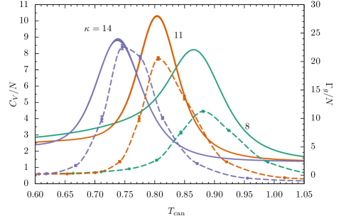
Figure 1: Canonical per-monomer fluctuations of energy $C_{V}/N=(1/N)d\langle E\rangle/dT_{\mathrm{can}}$ (solid lines) and square radius of gyration $\Gamma_{g}/N=(1/N)d\langle R^{2}_{g}\rangle/dT_{\mathrm{can}}$ (dashed lines) for a semiflexible polymer with 55 monomers as functions of the canonical heat-bath temperature at different values of the bending stiffness $\kappa$.

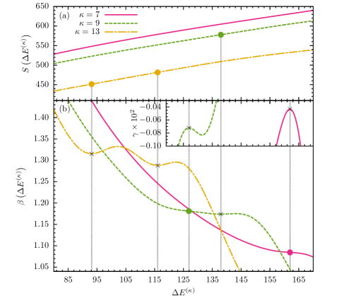
Figure 2: (a) Microcanonical entropies $S$ and (b) inverse temperatures $\beta$ as functions of the reduced energy $\Delta E^{(\kappa)}$ for different values of the bending stiffness $\kappa$. Least-sensitive inflection points indicating transitions are marked by dots. Corresponding extrema in the next-higher derivative are marked by crosses and support an easier identification of the transition point: Minima in $\beta$ indicate first-order transitions and maxima in $\gamma$ (inset) indicate second-order transitions. Dashed vertical lines help guide the eye from the inflection points to the corresponding extremum in the next-higher derivative commonly used to identify the transition energy.

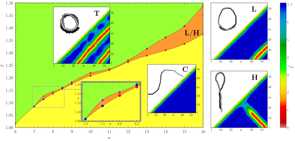
Figure 3: Hyperphase diagram for the semiflexible polymers with 55 monomers, parametrized by bending stiffness $\kappa$ and inverse microcanonical temperature $\beta$. Red diamonds mark first-order, blue dots second-order, and purple triangles third-order transitions. Solid transition lines are guides to the eye. Representative structures, characterizing the dominant types in the respective phases (C: wormlike random coils, H: hairpins, L: loops, T: toroids), and their distance maps (lower triangles in the insets) are also shown. Monomer labels are ordered from the black (first monomer) to the white end (last monomer).

In contrast, in the microcanonical inflection-point method [1] employed here, least-sensitive inflection points of the microcanonical entropy $S(E)=k_{\mathrm{B}}\ln\,g(E)$, where $g(E)$ is the density (or number) of system states at energy $E$, and its derivatives with respect to the energy are considered indicators of phase transitions. This has been motivated by the rapid change of thermodynamic quantities like the internal energy in the vicinity of canonical transition temperatures, which causes a maximally sensitive inflection point (a small variation in heat-bath temperature leads to a drastic response of the system). This results in a peak of the corresponding fluctuation or response quantity (which is why peaks in specific-heat curves like in Fig. 1 often serve as indicators of transitions in conventional canonical statistical analysis). However, in microcanonical statistical analysis the temperature is a system property. It is defined by $T(E)=[dS(E)/dE]^{-1}$ and, consequently, it is a function of the system energy. Therefore, the corresponding inflection point marking the transition in $T(E)$ is now least sensitive to changes in energy.

Extending this analogy in a systematic way, we classify a transition as of first order, if the entropy $S(E)$ exhibits a least-sensitive inflection point. Consequently, a second-order transition is characterized by a least-sensitive inflection point in the inverse microcanonical temperature $\beta(E)=dS(E)/dE$. For finite systems, higher-order transitions have to be considered seriously as well and are classified accordingly. As we will see later, third-order transitions, identified here by inflection points in $\gamma(E)=d^{2}S(E)/dE^{2}$, typically fill gaps near bifurcation points of transition lines.

It should also be noted that there are two transition categories, independent and dependent transitions [1]. However, in the model studied here, all transitions were found to be independent transitions, i.e., they are not entangled with other transition processes.

With this method, we recently found that even the two-dimensional Ising model possesses two third-order transitions in addition to the familiar second-order phase transition [1, 23]. Our method has already been successfully employed in previous studies of macromolecular systems [24, 25]. It has also proven useful in supporting the understanding of the general geometric and topological foundation of transitions in phase spaces [26, 27, 28, 29].

Microcanonical entropies $S(E)$ and inverse temperatures $\beta(E)$ are shown in Fig. 2 for various $\kappa$ values. The quantities are plotted as functions of the reduced energy $\Delta E^{(\kappa)}=E-E_{0}^{(\kappa)}$, where $E_{0}^{(\kappa)}$ is the ground-state energy estimate for the polymer with bending stiffness $\kappa$. The least-sensitive inflection points are marked by dots. For the actual quantitative identification of these inflection points, it is useful to search for extrema in the corresponding next-higher derivative. These extrema are marked by crosses.

For $\kappa=7$, we only find a single signal in the $\beta$ curve (and none in $S$), suggesting a single second-order transition in the plotted energy range. However, at $\kappa=9$, two different transitions emerge in close proximity: Least-sensitive inflection points in both $S$ and $\beta$ identify independent first- and second-order transitions. Most striking among these results are the two strong first-order transition signals found in the $\beta$ curve for $\kappa=13$.

Therefore, it is intriguing to construct the complete hyperphase diagram, parametrized by bending stiffness $\kappa$ and inverse microcanonical temperature $\beta$, in the vicinity of the bifurcation point. It is shown in Fig. 3 in this range of $\kappa$ values. We see that the coil-globule transition line, still intact from the flexible case ($\kappa=0$), begins to split into two branches at about $\kappa=7$. In fact, the structural behavior of the polymers changes qualitatively from there.

Transition points identified by microcanonical analysis of simulation data are marked by symbols. In the plotted region, the hyperphase diagram is clearly dominated by three phases. The disordered regime C is governed by wormlike random-coil structures. In this phase, entropic effects enable sufficiently large fluctuations that suppress the formation of stable energetic contacts between monomers. For $\kappa$ values just below the bifurcation, a direct transition into the toroidal phase T occurs as $\beta$ is increased beyond the transition point. However, more interestingly, a stable intermediate phase forms if $\kappa>7$. We characterize it as a mixed phase with hairpin (H) and loop (L) structures coexisting. Eventually, further cooling leads to another transition into the toroidal phase T. It is worth noting that upon increasing $\kappa$ beyond the bifurcation point, the upper line starts off with third-order transitions, then turning to second order, and eventually to first order. This is a typical characteristic feature of transition lines branching off a main line. Transitions of higher-than-second order are common in finite systems. Without their consideration, the phase diagram would contain gaps.

Exemplified simulations of longer chains with up to 100 monomers confirm the bifurcation of transition lines, but the bifurcation point shifts to larger $\kappa$ values and lower temperatures in this model, as expected.

The characterization of the phases was made simple by utilizing the distinct maps of pairwise monomer-monomer distances of the different structure types. Regions shaded red ($r_{nm}<1.2$) correspond to close contacts between monomers. Representative conformations for each phase are included in Fig. 3. The triangular maps shown underneath the structures exhibit the characteristic features of the class of structures they belong to. For extended coil-like structures prominent features are not present. Also, loops have only a small number of contacts near the tails, resulting in a short contact line parallel to the diagonal. In contrast, the toroidal structure possesses multiple windings and therefore an additional streak parallel to the diagonal appears. Hairpin structures are easily identified by the contact line that is perpendicular to the diagonal.

In order to quantify the population of the different structures in each phase, we have estimated the probabilities for each structure type in the energetic range that includes the two first-order transitions. Detailed results for $\kappa=16$ are shown in Fig. 4(a). To provide the context, we also included the $\beta$ curve as a dashed line. The two first-order transition regions are shaded in gray. The respective microcanonical Maxwell constructions define the coexistence regions of those transitions (shaded in gray in Fig. 4). They clearly do not overlap and leave an energetic gap, in which the intermediate mixed hairpin–loop crossover phase is located. This is also confirmed by the plot of the energy probability distributions $P_{\mathrm{can}}(E)=g(E)e^{-E/k_{\mathrm{B}}T_{\mathrm{can}}}/Z_{\mathrm{can}}$ (where $Z_{\mathrm{can}}=\int dEg(E)e^{-E/k_{\mathrm{B}}T_{\mathrm{can}}}$ is the canonical partition function) as shown in Fig. 4(b) for various canonical temperatures in the transition region. The envelope of these curves exhibits two noticeable suppression regions, where the inflection-point method indicated the first-order transitions.

Figure 4: (a) Microcanonical temperature and system energy dependence of frequencies for the different structure types at $\kappa=16$. (b) Canonical energy probability distributions $P_{\mathrm{can}}(E)$ at various inverse thermal energies $\beta_{\mathrm{can}}=1/k_{\mathrm{B}}T_{\mathrm{can}}$.

As expected, coil structures dominate at high energies, but their presence is rapidly diminished by the formation of more ordered hairpin structures. These conformations still provide sufficient entropic freedom for the dangling tail, which is already stabilized by van der Waals contacts, however. The loop part of the hairpin helps reducing the stiffness restraint. It is noteworthy that pure loop structures also significantly contribute to the population, although at a lesser scale in this region. The actual crossover from hairpins to loops happens within the intermediate phase, which is why we consider it a mixed phase. Even though hairpin and loop structures may be irrelevant at very low temperatures, they represent biologically significant secondary structure types at finite temperatures. The tail can be easily spliced, contact pair by contact pair, with little energetic effort, which supports essential micromolecular processes on the DNA and RNA level such as transcription and translation. The phase diagram shown in Fig. 3 tells us how important it is to discern the phase dominated by these structures.

Upon reducing the energy (and therefore also entropy), forming energetically favorable van der Waals contacts becomes the dominant structure formation strategy and loops coil in to eventually form toroids. Further lowering the energy toward the ground state may even lead to knotting [6, 7].

We would like to emphasize that we have also performed selected simulations of semiflexible chains in this generic model with 70 and 100 monomers, which essentially led to the same qualitative results. Quantitatively, we observe a shift of the bifurcation point toward higher bending stiffness values. This is expected, of course, as the number of possible energetic contacts scales with the number of monomers, which requires a larger energy penalty to break these symmetries. It also helps understand why microbiological structures are not only finite, but exist on a comparatively small, mesoscopic length scale. At the physiological scale, structure formation processes of large systems would be much more difficult to control and to stabilize. This also means that studying such systems in the thermodynamic limit may not help understanding physics at mesoscopic scales. Therefore, employing alternative statistical analysis methods as in this Letter is more beneficial than the application of standard procedures, however successful they have been in studies of other problems.

To conclude, neither canonical energetic nor structural fluctuation quantities hint at the existence of two clearly separated transitions for semiflexible polymers, which we could identify by microcanonical inflection point-analysis, though. Conventional canonical analysis is too rugged – the intermediate phase is simply washed out in the averaging process. This should be considered a problem, particularly when standard canonical analysis methods are employed in studies of finite systems. In the generic model for semiflexible polymers used in our Letter, the intermediate phase accommodates loop and hairpin structures, which are found in biomacromolecular systems including types of DNA and RNA. We conclude that bending stiffness is not only a necessary property of polymers in the formation of distinct and biologically relevant structures at finite temperatures; it also stabilizes the phase dominated by these structure types in a thermal environment, where entropy and energy effectively compete with each other. Neither flexible polymers nor crystalline structures would be equally adaptable and stable like semiflexible polymers are under physiological conditions. This is fully compliant with Nature’s governing principle, in which sufficient order is provided to enable the formation of stable mesostructures, but at the same time enough disorder allows these structures to explore variability. This makes them functional in a stochastic, thermal environment, with sufficient efficiency enabling lifeforms to exist and survive under these conditions.

We thank the Georgia Advanced Computing Resource Center at the University of Georgia for providing computational resources.

References

- [1] K. Qi and M. Bachmann, Phys. Rev. Lett. 120, 180601 (2018).
- [2] O. Kratky and G. Porod, J. Colloid Sci. 4, 35 (1949).
- [3] D. T. Seaton, S. Schnabel, D. P. Landau, and M. Bachmann, Phys. Rev. Lett. 110, 028103 (2013).
- [4] J. Zierenberg and W. Janke, Europhys. Lett. 109, 28002 (2015).
- [5] J. Wu, C. Cheng, G. Liu, P. Zhang, and T. Chen, J. Chem. Phys. 148, 184901 (2018).
- [6] S. Majumder, M. Marenz, S. Paul, and W. Janke, Macromolecules 54, 5321 (2021).
- [7] C. C. Walker, T. L. Fobe, and M. R. Shirts, Macromolecules 55, 8419 (2022).
- [8] B. Bird, C. F. Curtiss, R. C. Armstrong, and O. Hassager, Dynamics of Polymeric Liquids, 2nd ed. (Wiley, New York, 1987).
- [9] K. Kremer and G. S. Grest, J. Chem. Phys. 92, 5057 (1990).
- [10] A. Milchev, A. Bhattacharya, and K. Binder, Macromolecules 34, 1881 (2001).
- [11] K. Qi and M. Bachmann, J. Chem. Phys. 141, 074101 (2014).
- [12] M. Bachmann, Thermodynamics and Statistical Mechanics of Macromolecular Systems (Cambridge University Press, Cambridge, 2014).
- [13] R. H. Swendsen and J.-S. Wang, Phys. Rev. Lett. 57, 2607 (1986).
- [14] K. Hukushima and K. Nemoto, J. Phys. Soc. Jpn. 65, 1604 (1996).
- [15] K. Hukushima, H. Takayama, and K. Nemoto, Int. J. Mod. Phys. C 7, 337 (1996).
- [16] C. J. Geyer, in Computing Science and Statistics, Proceedings of the 23rd Symposium on the Interface, ed. by E. M. Keramidas (Interface Foundation, Fairfax Station, 1991), p. 156.
- [17] S. Schnabel, W. Janke, and M. Bachmann, J. Comput. Phys. 230, 4454 (2011).
- [18] A. M. Ferrenberg and R. H. Swendsen, Phys. Rev. Lett. 63, 1195 (1989).
- [19] S. Kumar, D. Bouzida, R. H. Swendsen, P. A. Kollman, and J. M. Rosenberg, J. Comput. Chem. 13, 1011 (1992).
- [20] B. A. Berg and T. Neuhaus, Phys. Lett. B 267, 249 (1991).
- [21] B. A. Berg and T. Neuhaus, Phys. Rev. Lett. 68, 9 (1992).
- [22] W. Janke, Physica A 254, 164 (1998).
- [23] K. Sitarachu and M. Bachmann, Phys. Rev. E 106, 014134 (2022).
- [24] D. Aierken and M. Bachmann, Polymers 12, 3013 (2020).
- [25] L. F. Trugilho and L. G. Rizzi, J. Stat. Phys. 186, 40 (2022).
- [26] G. Pettini, M. Gori, R. Franzosi, C. Clementi, and M. Pettini, Physica A 516, 376 (2019).
- [27] G. Bel-Hadj-Aissa, M. Gori, V. Penna, G. Pettini, and R. Franzosi, Entropy 22, 380 (2020).
- [28] M. Gori, R. Franzosi, G. Pettini, and M. Pettini, J. Phys. A: Math. Theor. 55 375002 (2022).
- [29] L. Di Cairano, J. Phys. A: Math. Theor. 55, 27LT01 (2022).