Possible origin of AT2021any: a failed GRB from a structured jet

Searching for afterglows not associated with any gamma-ray bursts (GRBs) is a longstanding goal of transient surveys. These surveys provide the very chance of discovering the so-called orphan afterglows. Recently, a promising orphan afterglow candidate, AT2021any, was found by the Zwicky Transient Facility. Here we perform multi-wavelength fitting of AT2021any with two different outflow models, namely the top-hat jet model and the structured Gaussian jet model. Although the two models can both fit the observed light curve well, it is found that the structured Gaussian jet model presents a better result, and thus is preferred by observations. In the framework of the Gaussian jet model, the best-fit Lorentz factor is about $68$, which indicates that AT2021any should be a failed GRB. The half-opening angle of the jet and the viewing angle are found to be 0.104 and 0.02, respectively, which means that the jet is essentially observed on-axis. The trigger time of the GRB is inferred to be about $1000$ s before the first detection of the orphan afterglow. An upper limit of $21.5\%$ is derived for the radiative efficiency, which is typical in GRBs.

1 Introduction

Gamma-ray bursts (GRBs) are energetic explosions occurring at cosmological distances. There are mainly two different phases in GRBs, the prompt emission and the follow-up afterglow phase (Piran 2004; Mészáros 2006; Kumar & Zhang 2015). The prompt emission usually peaks at sub-MeV (Fishman & Meegan 1995; Gruber et al. 2014), while the afterglow can be observed in a much broader wavelength ranging from soft X-rays to radio waves (Mészáros & Rees 1997; Sari et al. 1998; Zhang et al. 2006; Kann et al. 2010; Geng et al. 2016; Alexander et al. 2017; O’Connor et al. 2023). Generally speaking, the afterglow can last for a period ranging from days to years, whereas the prompt emission typically lasts for less than a few minutes. Despite the short duration of the prompt emission, the total energy released in $\gamma$-rays is enormous. For long-duration GRBs, the typical isotropic energy of the prompt emission is $10^{53}$ erg (Xu et al. 2023). Recently, the discovery of GRB 221009A has once again refreshed our perception of the energetics of GRBs (Ren et al. 2023; An et al. 2023; O’Connor et al. 2023; Sato et al. 2023; Yang et al. 2023). This event is found to have an isotropic energy of $\sim 10^{55}$ erg, which places it as the most energetic GRB in history (An et al. 2023; Yang et al. 2023).

For a typical GRB, both the prompt emission and the afterglow phases can be observed. However, there exist special cases of GRBs where the prompt emission is missing and only the afterglow phase could be observed. These afterglows are the so-called orphan afterglows (Rhoads 1997; Huang et al. 2002; Nakar et al. 2002; Zou et al. 2007; Gao et al. 2022). Theoretically, there are two different approaches to producing an orphan afterglow. First, if the initial Lorentz factor of the outflow is significantly less than $\sim 100$, the prompt emission will be too faint to be observed. Such explosions are also known as “failed GRBs” or “dirty fireballs” (Paczyński 1998; Dermer et al. 1999; Huang et al. 2002; Xu et al. 2012). Second, if the outflow is highly collimated (not isotropic), it is hard to detect the prompt emission when the explosion is viewed off-axis, i.e., the viewing angle is larger than the half-opening angle of the jet (Rhoads 1997; Nakar et al. 2002). In this case, the majority of $\gamma$-ray radiation from the GRB cannot be observed due to the relativistic beaming effect. However, the subsequent afterglow emission will be less beamed and can be visible to the observer in the afterglow stage (Rhoads 1997; Huang et al. 2002). These transients are called off-axis orphans.

It is also interesting to note a class of X-ray transients named X-ray flashes. Their temporal and spectral features of X-ray emissions are very similar to those of normal GRBs. The main difference is that X-ray flashes usually possess a significantly lower spectral peak energy than GRBs in the prompt emission phase. X-ray flashes can also be explained by the dirty fireball model (Huang et al. 2002) or the off-axis model (Yamazaki et al. 2002), which means they may be closely connected with orphan afterglows (Urata et al. 2015).

Assuming that all the orphan afterglows come from off-axis GRBs, we can estimate the half-opening angle of GRBs through the ratio between the orphan afterglow rate and GRB rate (Rhoads 1997; Paczyński 2000). However, as pointed out by Huang et al. (2002), there should be many orphan afterglows coming from failed GRBs since the baryon loading issue widely exists in popular progenitor models of GRBs (Piran 2004). Therefore the estimation above may not be very straightforward.

On the other hand, searching for orphan afterglows is not an easy task (Grindlay 1999; Greiner et al. 2000; Levinson et al. 2002; Rau et al. 2006; Gal-Yam et al. 2006; Khabibullin et al. 2012; Ho et al. 2018; Huang et al. 2020; Ho et al. 2022; Leung et al. 2023). So far, only six orphan afterglow candidates have been reported. One of them was found at radio wavelength by the Very Large Array (VLA): FIRST J$141918.9+394036$ (Law et al. 2018; Mooley et al. 2022). Its radio evolution and the lack of associated GRB suggest that it might be an off-axis orphan afterglow (Mooley et al. 2022). The other five transients are all found in optical bands. They are PTF11agg (Cenko et al. 2013; Wang & Dai 2013; Wu et al. 2014) discovered by the Palomar Transient Factory (Law et al. 2009), and AT2019pim (Kool et al. 2019), AT2020blt (Ho et al. 2020; Andreoni et al. 2021; Sarin et al. 2022), AT2021any (Ho et al. 2022; Gupta et al. 2022), and AT2021lfa (Ho et al. 2022; Lipunov et al. 2022) discovered by the Zwicky Transient Facility (ZTF; Bellm et al. (2019)).

With the currently available observational data, it is still a challenge to derive the physical parameters and reveal the nature of an orphan afterglow. A major problem is the lack of the trigger time of the unseen GRB potentially associated with the afterglow. Usually, the trigger time is estimated by fitting the observed light curve with a particular model (Ho et al. 2020; Gupta et al. 2022; Ho et al. 2022). Recently, Sarin et al. (2022) used the last non-detection information from an upper limit in the $r$ band to constrain the trigger time. However, the non-detection may result from bad seeing or other interferences, thus cannot provide decisive information on the trigger time.

In this study, we present an in-depth study on AT2021any, an orphan afterglow candidate found by ZTF. The trigger time, together with other parameters, will be derived by fitting the observed light curve. An efficient code is developed for this purpose. Synchrotron emission and synchrotron self-Comptonization (SSC) are considered in our modeling. The effect of synchrotron self-absorption is also included.

Our paper is organized as follows. First, the multi-wavelength observational data of AT2021any are collected and presented in Section 2. The physical models used to fit the data are then briefly described in Section 3. In Section 4, we present the fitting results of AT2021any with different approaches and compare the goodness of fitting. Finally, conclusions and discussion are presented in Section 5.

2 Observational data of AT2021any/ZTF21aayokph

AT2021any/ZTF21aayokph was discovered on $06$:$59$:$45.6$ UTC $2021$ January $16$ by ZTF (Ho et al. 2021). It had an $r$ band magnitude of $r=17.92\pm 0.06$ mag when it was first detected. The most recent non-detection was only $20.3$ minutes before the first detection (Ho et al. 2022), which gives a limiting magnitude of $r>20.28$ mag. No associated GRB was recorded during the period between the last non-detection and the first detection (Ho et al. 2022; Gupta et al. 2022). The object faded rapidly in the $r$ band, with a fading rate of $14$ mag day ^-1 during the first $3.3$ hours. The extinction-corrected color index was found to be $g-r=(0.25\pm 0.19)$ mag (Ho et al. 2022). These observations place AT2021any as a promising orphan afterglow candidate. Using spectroscopic observations, the redshift of AT2021any was later determined as $z=2.5131\pm 0.0016$ (de Ugarte Postigo et al. 2021; Ho et al. 2022). AT2021any was subsequently followed by a variety of optical facilities (see Ho et al. (2022) and Gupta et al. (2022) for more information). The multi-wavelength optical photometry data are collected and listed in Table 1. Note that the AB magnitudes in Table 1 are not corrected for the extinction of the Milky Way.

The object was followed in X-rays by Swift-XRT (Ho & Zwicky Transient Facility Collaboration 2021). The observations were performed in three different epochs, with a total exposure time of $8.2$ ks. X-ray emission was detected only in the first epoch. The unabsorbed flux density is estimated as $3.30\times 10^{-13}$ erg cm^-2 s^-1, with a neutral hydrogen column density of $N_{\rm{H}}=8.12\times 10^{20}$ cm^-2 (Willingale et al. 2013) and an assumed photon index of $\Gamma_{\rm{p}}=2$ (see Table 2).

The transient was observed in radio by VLA (Perley et al. 2021; Ho et al. 2022). Eight epochs of observations were performed from $4.90$ days to $75.77$ days after the discovery of AT2021any. We have collected the radio data obtained by Ho et al. (2022) and listed them in Table 3.

3 Dynamics and emission mechanisms of GRBs

In this section, we briefly describe the dynamic evolution and radiation process of relativistic outflows that produce GRBs. The dynamics of the outflow can be depicted by the following equations (Huang et al. 2000a, 2006; Geng et al. 2013; Xu et al. 2022)

$$\frac{dR}{dt}=\beta c\Gamma(\Gamma+\sqrt{\Gamma^{2}-1}),$$ (1)

$$\frac{dm}{dR}=2\pi R^{2}(1-\cos\theta_{\rm{j}})nm_{\rm{p}},$$ (2)

$$\frac{d\Gamma}{dm}=-\frac{\Gamma^{2}-1}{M_{\rm{ej}}+\epsilon_{\rm{r}}m+2(1-\epsilon_{\rm{r}})\Gamma m}.$$ (3)

Note that the lateral expansion of the outflow is neglected in our calculation. Here, $R$ is the shock radius in the GRB rest frame, $c$ is the speed of light, and $\Gamma$ is the Lorentz factor of the outflow with $\beta=\sqrt{\Gamma^{2}-1}/\Gamma$. $t$ is the observer’s time. $m$ is the swept-up mass of the interstellar medium (ISM), $\theta_{\rm{j}}$ is the half-opening angle of the outflow, and $m_{\rm{p}}$ is the proton’s mass. $n$ is the number density of the surrounding ISM. For a homogeneous ISM, we take $n$ as a constant. As for a wind ISM, we have $n=Ar^{-2}$, where $A$ is a coefficient depending on the mass loss rate and the speed of the wind (Chevalier & Li 1999; Dai & Lu 2001; Wu et al. 2003; Ren et al. 2023). $M_{\rm{ej}}$ is the initial mass of the ejecta and $\epsilon_{\rm{r}}$ is the radiative efficiency. In this study, note that when we calculate the dynamical evolution of a structured jet, our method is to divide the whole jet into many mini-jets. For a mini-jet located at angle $\theta$, Equation 2 should then be modified as $\frac{dm}{dR}=\sin\theta d\theta d\phi R^{2}nm_{\rm{p}}$ to calculate the swept-up mass, where $d\theta$ is the angular length of the mini-jet and $d\phi$ is its width.

Synchrotron radiation from shock-accelerated electrons is involved in GRB afterglows (Sari et al. 1998). We use the superscript prime ($\prime$) to denote the quantities in the shock comoving frame, while those without prime are in the observer frame. In the fast-cooling regime, the flux $F_{\nu^{\prime}}$ at frequency $\nu^{\prime}$ is

$$F_{\nu^{\prime}}=F_{\nu^{\prime},\rm{max}}\left\{\begin{array}[]{ll}(\frac{\nu^{\prime}}{\nu_{\rm{c}}^{\prime}})^{\frac{1}{3}},&\nu^{\prime}<\nu_{\rm{c}}^{\prime},\\ (\frac{\nu^{\prime}}{\nu_{\rm{c}}^{\prime}})^{\frac{1}{2}},&\nu_{\rm{c}}^{\prime}<\nu^{\prime}<\nu_{\rm{min}}^{\prime},\\ (\frac{\nu^{\prime}}{\nu_{\rm{min}}^{\prime}})^{-\frac{p}{2}}(\frac{\nu_{\rm{c}}^{\prime}}{\nu_{\rm{min}}^{\prime}})^{\frac{1}{2}},&\nu_{\rm{min}}^{\prime}<\nu^{\prime}<\nu_{\rm{max}}^{\prime},\end{array}\right.$$ (4)

where $\nu_{\rm{c}}^{\prime}$, $\nu_{\rm{min}}^{\prime}$, and $\nu_{\rm{max}}^{\prime}$ are characteristic frequencies corresponding to the cooling Lorentz factors $\gamma_{c}^{\prime}$, the minimum Lorentz factor $\gamma_{\rm{min}}^{\prime}$, and maximum Lorentz factor $\gamma_{\rm{max}}^{\prime}$, respectively. $p$ is the electron spectral index and $F_{\nu^{\prime},\rm{max}}$ is the peak flux density (Sari et al. 1998).

In the slow-cooling regime, when $\nu_{\rm{min}}^{\prime}<\nu^{\prime}<\nu_{\rm{max}}^{\prime}$, we have

$$F_{\nu^{\prime}}=F_{\nu^{\prime},\rm{max}}\left\{\begin{array}[]{ll}(\frac{\nu^{\prime}}{\nu_{\rm{min}}^{\prime}})^{\frac{1}{3}},&\nu^{\prime}<\nu_{\rm{min}}^{\prime},\\ (\frac{\nu^{\prime}}{\nu_{\rm{min}}^{\prime}})^{\frac{1-p}{2}},&\nu_{\rm{min}}^{\prime}<\nu^{\prime}<\nu_{\rm{c}}^{\prime},\\ (\frac{\nu^{\prime}}{\nu_{\rm{c}}^{\prime}})^{-\frac{p}{2}}(\frac{\nu_{\rm{c}}^{\prime}}{\nu_{\rm{min}}^{\prime}})^{\frac{1-p}{2}},&\nu_{\rm{c}}^{\prime}<\nu^{\prime}<\nu_{\rm{max}}^{\prime}.\end{array}\right.$$ (5)

In the case of $\nu_{\rm{max}}^{\prime}<\nu_{\rm{c}}^{\prime}$, we have

$$F_{\nu^{\prime}}=F_{\nu^{\prime},\rm{max}}\left\{\begin{array}[]{ll}(\frac{\nu^{\prime}}{\nu_{\rm{min}}^{\prime}})^{\frac{1}{3}},&\nu^{\prime}<\nu_{\rm{min}}^{\prime},\\ (\frac{\nu^{\prime}}{\nu_{\rm{min}}^{\prime}})^{\frac{1-p}{2}},&\nu_{\rm{min}}^{\prime}<\nu^{\prime}.\end{array}\right.$$ (6)

We use the Compton parameter $Y$ to denote the ratio of the inverse Compton scattering luminosity with respect to synchrotron luminosity. It can be calculated as

$$Y=\frac{-1+\sqrt{1+4\epsilon_{\rm{r,e}}\epsilon_{\rm{e}}\epsilon_{B}}}{2}.$$ (7)

Here $\epsilon_{\rm{r,e}}$ is the fraction of the electron energy that was radiated, while $\epsilon_{\rm{e}}$ is the fraction of thermal energy carried by electrons and $\epsilon_{B}$ is the ratio of magnetic field energy to the total energy (Sari & Esin 2001; Wei et al. 2006).

The synchrotron self-absorption effect is also considered in our calculations. As a result, the observed flux should be corrected by multiplying a factor of $f(\tau_{\nu^{\prime}})=(1-e^{-\tau_{\nu^{\prime}}})/\tau_{\nu^{\prime}}$, where $\tau_{\nu^{\prime}}$ is the optical depth. The self-absorption coefficients and the optical depth are calculated by following Wu et al. (2003) and Geng et al. (2016).

The observed flux density at frequency $\nu$ can be calculated as

$$F_{\nu}(\Theta)=(1+z)\mathcal{D}^{3}f(\tau_{\nu^{\prime}})F_{\nu^{\prime}},$$ (8)

where $\Theta$ stands for the angle between the velocity of emitting material and the line of sight. $\mathcal{D}=1/[\Gamma(1-\beta\cos\Theta)]$ is the Doppler factor and $\nu^{\prime}=(1+z)\nu/\mathcal{D}$. To calculate the observed flux $F_{\nu}(t)$ at a given time $t$, we need to integrate the emission power over the equal arrival time surface (EATS), which is determined by

$$t=(1+z)\int\frac{1-\beta\cos\Theta}{\beta c}dR.$$ (9)

4 Multi-wavelength fitting of the afterglow

In this section, we present multi-wavelength fitting of AT2021any by considering two different models. First, a simple top-hat jet model is used, which has a constant energy per solid angle and a uniform Lorentz factor within the jet. Secondly, we consider a structured jet model with a Gaussian profile (Kumar & Granot 2003; Troja et al. 2018; Geng et al. 2019; Lamb et al. 2021). In this case, the distribution of the kinetic energy is taken as $E(\theta)=E_{\rm{k,iso}}\exp(-\theta^{2}/\theta_{\rm{c}}^{2})$ at angle $\theta$, and the profile of the Lorentz factor is assumed to take the form of $\Gamma(\theta)=(\Gamma_{0}-1)\exp(-\theta^{2}/2\theta_{\rm{c}}^{2})+1$. Here $E_{\rm{k,iso}}$ is the isotropic equivalent energy on the jet axis ($\theta=0$) and $\Gamma_{0}$ is the corresponding Lorentz factor. $\theta_{\rm{c}}$ stands for the half-opening angle of the jet core. For convenience, we assume that the jet is cut off at an angle of $\theta_{\rm{j}}$, i.e., $E(\theta)=0$ and $\Gamma(\theta)=1$ for $\theta>\theta_{\rm{j}}$. In other words, $\theta_{\rm{j}}$ effectively denotes the edge of the structured jet.

The observed broadband X-ray flux data are converted to the flux at the frequency of $\nu=1\times 10^{18}$ Hz. To do so, a photon index of $\Gamma_{\rm{p}}=2$ is applied (Ho et al. 2022). In the optical bands, we consider a Galactic extinction of $E(B-V)=0.0575$ mag (Schlafly & Finkbeiner 2011) to convert the observed magnitudes to flux densities. The radio afterglow data in four different bands are also used in our fitting, i.e., S(3GHz), C(6GHz), X(10GHz), and Ku(15GHz) bands.

We use the Markov Chain Monte Carlo (MCMC) algorithm to get the best-fit results for the multi-wavelength afterglow of AT2021any. The parameters derived for different models are shown in Table 4. The shift time of the light curve   is defined as the time interval between the GRB trigger and the first observation. This parameter is introduced to find out the most probable trigger time of the GRB associated with AT2021any. A constant ISM density is considered here for simplicity.

4.1 The top-hat jet model

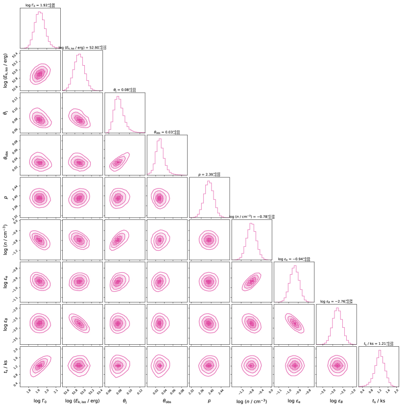
(a)

Figure 1: Parameters derived for AT2021any by using the top-hat jet model ($1\sigma-3\sigma$ confidence levels are shown). The best-fit results are marked with $1\sigma$ uncertainties above the panel of their posterior distribution.

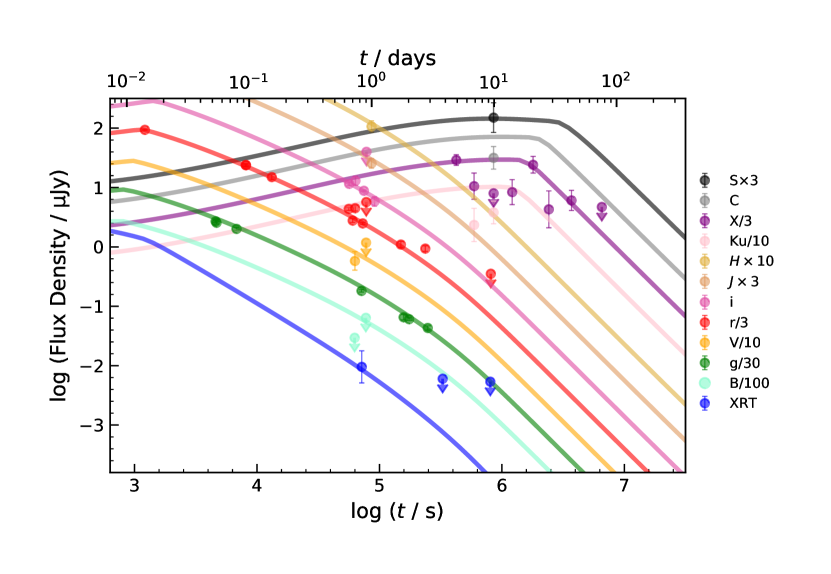
(a)

Figure 2: Observed multi-wavelength afterglow of AT2021any and the best-fit result by using the top-hat jet model (solid curves). The dashed line represents the broken power law fitting result of the $r$ band data.

We begin our fitting with the top-hat jet model. The numerical results are presented in Table 4 and the corresponding corner plot is shown in Figure 1. The best-fit value for the initial Lorentz factor of the jet ($\Gamma_{0}$) is $\sim 83$, which favors a failed GRB origin. Note that the Lorentz factor is generally sensitive to the early afterglow, especially its onset. In the case of AT2021any, although the onset of the afterglow was not clearly detected, the most recent non-detection was luckily only 20.3 minutes before the first detection. It gives a firm constraint on the onset of the afterglow. This is the reason that the Lorentz factor can be effectively inferred from the observations. The multi-wavelength observational data points and the best-fit light curves are plotted in Figure 2. We see that the X-ray and optical data are generally well-fitted. However, the radio data seem to somewhat deviate from the theoretical light curves. Note that the effect of interstellar scintillation is not included in our calculations. Small-scale inhomogeneities in the ISM can cause scintillation by changing the phase of radio waves. The line of sight to a distant source also shifts as the Earth moves, leading to radio flux fluctuations. The scattering effect will be significant when the radio frequency is smaller than the transition frequency. In fact, Ho et al. (2022) pointed out that interstellar scintillation may have a significant contribution to the radio afterglow of AT2021any. They calculated the transition frequency at the direction of AT2021any and got a result of $15$ GHz by using the NE2001 model (Cordes & Lazio 2002). Therefore, the radio light curves we considered here could be largely affected by interstellar scintillation.

In Figure 2, we see that the optical light cures have an obvious break at about $t_{\rm{b}}\sim 0.4$ days. Before this time, the temporal index is about $\alpha_{\rm{opt},1}=-0.75\pm 0.1$, while it becomes $\alpha_{\rm{opt},2}=-1.33\pm 0.23$ after the break time. Note that $\alpha_{\rm{opt},2}$ is satisfactorily consistent with the result expected for the fireball model (Sari et al. 1998), i.e. $-(3p-2)/4=-1.3$ for $p\sim 2.4$ from our best fit. It indicates that the optical band has crossed the cooling frequency at around $0.4$ days. The theoretical temporal index before the optical band crosses the cooling frequency should be $-3(p-1)/4=-1.05$. It is smaller than the observed value of $\alpha_{\rm{opt},1}=-0.75$ as mentioned above. The difference may be due to the EATS effect, which is more significant at the early stages of the afterglow.

In Figure 2, the half-opening angle of the jet is found to be $0.08^{+0.01}_{-0.01}$, while the viewing angle is $0.03^{+0.01}_{-0.01}$. It indicates that we are essentially observing the jet on the axis. An achromatic jet break could be seen in the optical light curves and the temporal decay index is around $-2$ after the jet break. The break time is about $\sim 2$ days, which is also roughly consistent with the theoretically jet break time of $t_{\rm{j}}\sim 1.2\frac{(1+z)}{2}E_{\rm{k,iso},53}^{1/3}n^{-1/3}\theta_{\rm{j},-1}^{8/3}=1.96$ days (Sari et al. 1999).

Note that the decay index of our theoretical X-ray light curve is around $1.3$ between $0.01$ and $1$ day. It is obviously steeper than the optical light curves in the same period. This is easy to understand. The frequencies of X-ray photons are much higher than that of optical photons. As a result, it is in the fast cooling regime (i.e., the frequency is higher than the characteristic cooling frequency). Then, the theoretical decay index should be $\sim-(3p-2)/4=1.3$ (Sari et al. 1998), which is well consistent with our numerical result. SSC might have some effects on the X-ray afterglow. Here we present some further discussions on this issue. The effect of SSC can be assessed by the Compton parameter $Y$, which is defined as the ratio of the inverse Compton scattering luminosity with respect to the synchrotron luminosity. As shown in Eq. (7), $Y$ is sensitively dependent on $\epsilon_{\rm{r,e}}$, i.e., the fraction of the radiated electron energy. According to Sari & Esin (2001), $\epsilon_{\rm{r,e}}$ takes the form of $\epsilon_{\rm{r,e}}=(\frac{\gamma_{\rm{min}}}{\gamma_{c}})^{p-2}$ considering that the bulk of electrons are in the slow-cooling regime at the afterglow phase. It can be further expressed as $\epsilon_{\rm{r,e}}=(1.27\times 10^{-8}\frac{p-2}{p-1}\epsilon_{\rm{e}}\epsilon_{B}\Gamma^{4}t)^{p-2}$ (Huang et al. 2000b). Taking $\Gamma\propto t^{-3/8}$ for the adiabatic expansion case (Sari et al. 1998) and combining the best-fit parameters for the top-hat jet discussed here, we finally have $\epsilon_{\rm{r,e}}\sim 0.007t^{-0.2}$. Consequently, we get $Y=\frac{-1+\sqrt{1+4.76t^{-0.2}}}{2}$ from Eq. (7). We see that the value of $Y$ will decrease from $Y=0.35$ at $t=100$ s to $Y=0.16$ at $t=10000$ s. Therefore SSC will generally have a negligible effect on the afterglow of AT2021any.

The radio light curve peaks at about $20$ days. The pre-peak temporal index of the radio light curve is about $1/2$. It indicates that the radio emission will reach the peak flux when the observed radio frequency crosses the characteristic frequency of $\nu_{\rm{min}}$ (Zhang 2018). The post-peak radio light curve is dominated by the jet break effect. Here we further address the effect of synchrotron self-absorption, which is mainly determined by the synchrotron self-absorption frequency ($\nu_{\rm{a}}$). Following Gao et al. (2013), we can derive the self-absorption frequency as $\nu_{\rm{a}}=1.03\times 10^{9}$ Hz in the case of $\nu_{\rm{a}}<\nu_{\rm{min}}<\nu_{\rm{c}}$. On the other hand, it will be $\nu_{\rm{a}}=8.3\times 10^{12}(\frac{t}{s})^{-0.72}$ Hz in the case of $\nu_{\rm{min}}<\nu_{\rm{a}}<\nu_{\rm{c}}$. In both cases, we see that $\nu_{\rm{a}}$ is in the radio ranges. Thus the synchrotron self-absorption will mainly affect the radio afterglow light curves and will have a negligible effect on the optical and X-ray light curves.

4.2 The structured jet model

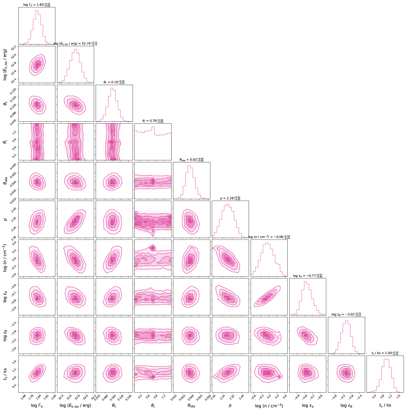
(a)

Figure 3: Parameters derived for AT2021any by using the structured jet model ($1\sigma-3\sigma$ confidence levels are shown). The best-fit results are marked with $1\sigma$ uncertainties above the panel of their posterior distribution.

We have also tried to fit the observational data with a structured jet. The best-fit results are presented in Table 4, and the corresponding corner plot is shown in Figure 3. We see that the best-fit $\Gamma_{0}$ value is $\sim 68$, which is still a typical Lorentz factor for a failed GRB. The geometry parameters are derived as $\theta_{\rm{c}}=0.10\pm 0.01$, $\theta_{\rm{j}}=0.76^{+0.50}_{-0.46}$, and $\theta_{\rm{obs}}=0.02^{+0.003}_{-0.002}$. An on-axis viewing angle is still favored here. Figure 3 shows that the error bar of $\theta_{\rm{j}}$ is relatively large. This is due to the fact that the radiation from materials outside the jet core contributes little to the observed emissions, which means that the observed flux is insensitive to $\theta_{\rm{j}}$. In fact, at the early stage, we could only see a small fraction of the jet due to the beaming effect. As the jet decelerates, the Lorentz factor is decreasing and we could see a larger area of the jet. However, the Lorentz factor of the materials outside the jet core will be too small to produce significant emissions at later stages, leading to a steep decay in the afterglow light curve. We derive $E_{\rm{k,iso}}\sim 5.50\times 10^{52}$ erg, $p\sim 2.3$, $\epsilon_{\rm{e}}\sim 0.17$, and $\epsilon_{B}\sim 0.001$ for the structured jet model. These parameter values are similar to those of the top-hat jet model. As for the ambient density $n$, the structured jet model requires a relatively larger value of $n\sim 0.87$ cm^-3 as compared to $n\sim 0.16$ cm^-3 for the top-hat jet model. It indicates that a cleaner circum-burst environment is needed for the top-hat jet model. In the framework of the structured jet model, the best-fit shift time is about $\thinspace\sim 1000$ s, which is $\sim 200$ s smaller than that obtained for the top-hat jet model.

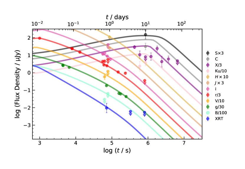
(a)

Figure 4: Observed multi-wavelength afterglow of AT2021any and the best-fit result by using the structured jet model (solid curves). The dashed line represents the broken power law fitting result of the $r$ band data.

The observational data points are compared with the best-fit light curves of the structured jet model in Figure 4. Similar to Figure 2, we see that the observed radio data points show significant fluctuations and thus could not be satisfactorily fit by the theoretical light curves (especially in the C band). Again, it may be due to the interstellar scintillation effect. The theoretical $r$ band optical light curve still possesses a shallow decay, with a timing index of $-0.69\pm 0.01$ before $t_{\rm{b}}\sim 0.35$ days. It is slightly larger than the analytical value of $-3(p-1)/4=-0.975$ and may be due to the EATS effect. After $t_{\rm{b}}\sim 0.35$ days, the timing index is $-1.33$, which is roughly consistent with the analytical result of $\sim-(3p-2)/4=-1.225$. The jet break time is about $2$ days for the structured jet model.

4.3 Comparing the goodness of fitting

We have assessed the goodness of fitting for different models. Two tests are performed for this purpose. First, we use the reduce-$\chi^{2}$, which is calculated as

$$\chi^{2}/\rm{d.o.f.}=\sum_{i}\frac{(\log f_{\rm{th},i}-\log f_{\rm{obs},i})^{2}}{\sigma_{i}^{2}}\times\frac{1}{\rm{d.o.f.}},$$ (10)

where the degree of freedom (d.o.f.) is defined as the difference between the number of observational data points and the model parameters. $f_{\rm{th},i}$ and $f_{\rm{obs},i}$ are the theoretical flux density and the observed flux density at the time of $t_{i}$, while $\sigma_{i}$ represents the error bar for each data point. The reduced-$\chi^{2}$ for each model is presented in Table 4. We find that the structured jet model has a relatively lower reduced-$\chi^{2}$, suggesting that it is the preferred model.

The second test is conducted by performing the Bayesian Information Criterion (BIC) method (Schwarz 1978). BIC is defined as

$$\rm{BIC}=-2\ln\mathcal{L}(P)+k\ln(N),$$ (11)

where $N$ is the number of observational data points and $k$ is the number of model parameters. Here $P$ stands for a set of the model parameters and $\mathcal{L}$ is the maximized value of the likelihood function. The likelihood function takes the form of (Xu et al. 2021)

$$\mathcal{L}(P)=\prod_{i}\frac{1}{\sqrt{2\pi}\sigma_{i}}\exp\left[-\frac{1}{2}\frac{(\log f_{\rm{th},i}-\log f_{\rm{obs},i})^{2}}{\sigma_{i}^{2}}\right].$$ (12)

According to the BIC test, the model which provides the minimum BIC score should be the preferred model. Usually, the BIC score is compared through $\Delta$BIC values, i.e., the difference between the best model and other models. We list the $\Delta$BIC score for each model in Table 4. Again we see that the structured jet scenario is better than the top-hat jet scenario.

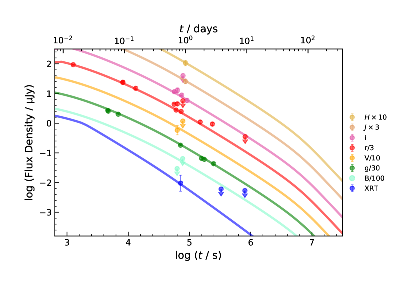
(a)

Figure 5: Observed and theoretical optical and X-ray afterglow of AT2021any. The solid curves represent the best-fit results obtained from optical and X-ray data by using the top-hat jet model.

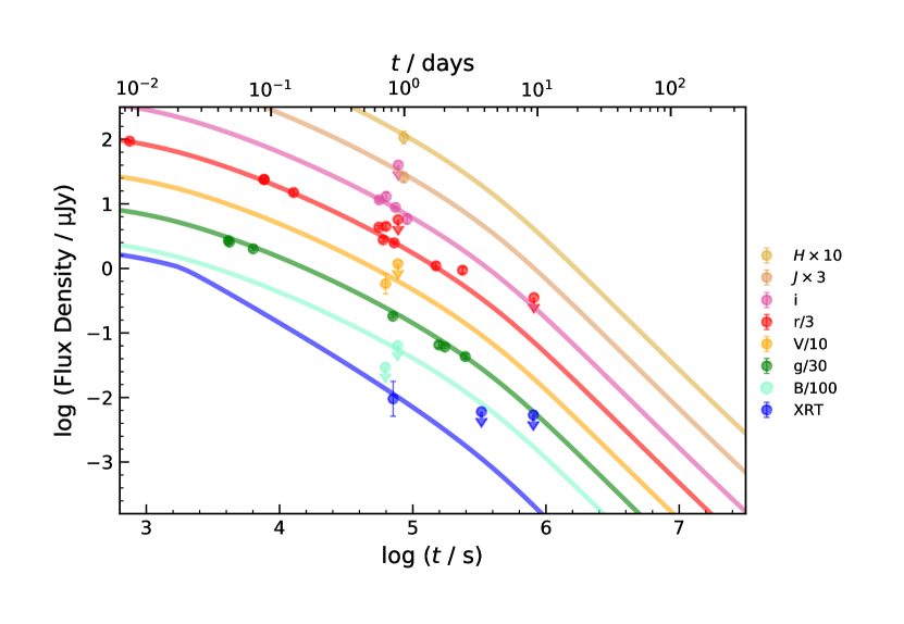
(a)

Figure 6: Observed and theoretical optical and X-ray afterglow of AT2021any. The solid curves represent the best-fit results obtained from optical and X-ray data by using the structured jet model.

Radio afterglows are largely affected by interstellar scintillation. The random fluctuation of radio flux may affect the goodness of fitting. To avoid the uncertainties caused by this factor, we have performed the model fitting by excluding all the radio data. The parameters derived are also presented in Table 4. Figure 5 and Figure 6 show the best-fit light curves for the top-hat and structured jet models, respectively. For the top-hat jet model, the geometry parameters differ significantly from the previous results when the radio data are included. The best-fit angles are $\theta_{\rm{j}}=0.17^{+0.03}_{-0.04}$ and $\theta_{\rm{obs}}=0.12^{+0.04}_{-0.04}$ now, which are relatively larger. Still, an on-axis scenario is favored. Other parameters such as $\Gamma_{0},E_{\rm{k,iso}},p,n,\epsilon_{\rm e},\epsilon_{\rm B},t_{\rm s}$ do not change too much. As for the structured jet model, the major difference induced by excluding the radio data is about the shift time. We get the new shift time as $\thinspace\sim 750$ s, which is $250$ s smaller than the previous value derived by including the radio data. Apart from this difference, the best-fit values for the other parameters are essentially similar. Finally, from both the reduce-$\chi^{2}$ test and the BIC test, the structured jet model is still preferred after excluding the radio data, thus the main conclusion remains unchanged.

To summarize, according to the above two tests, AT2021any is best described by the structured jet model. This conclusion is supported either the radio data, which are affected by interstellar scintillation, are included or excluded. Additionally, our results suggest that AT2021any should be an on-axis failed GRB.

5 Conclusions and discussion

Searching for orphan afterglows is a difficult but meaningful task. By fitting the multi-wavelength afterglow data, we will get a better understanding of the physics of orphan afterglows. In this study, two different kinds of outflows are applied to the orphan afterglow candidate of AT2021any, i.e. a top-hat jet and a structured Gaussian jet. It is found that the structured Gaussian jet model presents the best fit to the multi-wavelength light curves of AT2021any. According to our modeling, the trigger time of the GRB associated with AT2021any is about $1000$ s prior to the first detection.

In the framework of the structured Gaussian jet model, the isotropic kinetic energy is derived as $5.50\times 10^{52}$ erg. From this kinetic energy, we could estimate the $\gamma$-ray efficiency $\eta$ of the unseen GRB associated with AT2021any. The source was in the field of view of Fermi-GBM but was undetected by the instrument (Ho et al. 2022), which places a firm upper limit on the peak $\gamma$-ray flux as $\sim 1\times 10^{7}$ erg s^-1 cm^-2. Then the corresponding upper limit of the peak luminosity is $L_{\rm{p}}\lesssim 5.31\times 10^{51}$ erg s^-1 for a redshift of $z=2.513$. The upper limit of the isotropic $\gamma$-ray energy will be $E_{\gamma,\rm{iso}}=L_{\rm{p}}*T_{90}/(1+z)\lesssim 1.51\times 10^{52}$ erg for a typical burst duration of $T_{90}=10$ s (for long GRBs). So, we can get the $\gamma$-ray efficiency as $\eta=E_{\gamma,\rm{iso}}/(E_{\gamma,\rm{iso}}+E_{\rm{k,iso}})\lesssim 21.5\%$, which is roughly consistent with the result derived by Gupta et al. (2022) ($\eta\lesssim 28.6\%$). Note that the $\gamma$-ray efficiency derived here is typical for long GRBs. Some long GRBs could even have much higher $\gamma$-ray efficiencies but still could be explained by the photosphere model (Rees & Mészáros 2005; Pe’er 2008) or the internal-collision-induced magnetic reconnection and turbulence (ICMART) model (Zhang & Yan 2011; Zhang & Zhang 2014).

A relativistic fireball with a lower initial Lorentz factor is usually optically thick at the internal shock radius, but it becomes optical thin at the external radius. In other words, the photosphere radius of a dirty fireball is much larger than the internal shock radius and is much smaller than the external shock radius. In the case of AT2021any, we have $\Gamma_{0}\sim 68$, $E_{\rm{k,iso}}\sim 5.50\times 10^{52}$ erg, and $n\sim 0.87$ cm^-3 as derived from the structured Gaussian jet model. Let us consider two mini-shells ejected with a separation time of $\delta t\sim 10^{-3}$ s. The internal shock radius can be obtained as $R_{\rm{IS}}\sim 2\Gamma_{0}^{2}c\delta t=2.69\times 10^{11}$ cm (Rees & Mészáros 1994). The optical depth is dominated by electron scattering for $\Gamma_{0}<10^{5}$ (Mészáros et al. 1993), which can be calculated as $\tau_{\rm{T}}=\frac{E_{\rm{k,iso}}\sigma_{\rm{T}}}{8\pi N_{\rm{sh}}R\delta Rc^{2}m_{\rm{p}}\Gamma_{0}^{3}}$ (Mészáros & Rees 2000; Zhang 2018). Here $\sigma_{\rm{T}}$ is the electron Thomson cross-section, $N_{\rm{sh}}$ stands for the number of all the mini-shells, and $\delta R\sim 3\times 10^{7}$ cm is their typical width. Taking the burst duration as $T_{90}=10$ s and assuming $N_{\rm{sh}}\sim T_{90}/\delta t=10^{4}$, we can get the photosphere radius as $R_{\rm{ph}}=\frac{E_{\rm{k,iso}}\sigma_{\rm{T}}}{8\pi N_{\rm{sh}}\delta Rc^{2}m_{\rm{p}}\Gamma_{0}^{3}}=1.09\times 10^{13}$ cm for $\tau_{\rm{T}}=1$. At the same time, the external shock radius is $R_{\rm{ext}}=\left(\frac{3E_{\rm{k,iso}}}{2\pi nm_{\rm{p}}c^{2}\Gamma_{0}^{2}}\right)^{1/3}=1.65\times 10^{17}$ cm (Rees & Mészáros 1992; Zhang 2018). Comparing these radii, we find that they satisfy $R_{\rm{IS}}<R_{\rm{ph}}<R_{\rm{ext}}$. It indicates that for AT2021any, the synchrotron radiation of $\gamma$-rays in the prompt emission phase is invisible to us due to the optically thick condition, which is consistent with observational constraints. However, emission in the afterglow phase could be observed since it is optically thin at late stages.

Our model does not include the impact of a reverse shock. Usually, an optical orphan afterglow would be found at the early stage of the burst, when the smoking gun is still relatively bright. At this stage, the optical emission of the afterglow may be affected by the reverse shock (Wu et al. 2003; Wang & Dai 2013). Note that the reverse shock component may help us better constrain the physical parameters of an orphan afterglow. Wang & Dai (2013) engaged the reverse shock emission from a post-merger millisecond magnetar to explain the light curves of PTF11agg, another orphan afterglow candidate. They argued that the multi-wavelength light curves can be better fitted by adding a reverse shock component. Anyway, in the case of AT2021any studied here, no clear evidence supporting the existence of a reverse shock is spotted. The reason may be that the first detection is about 1000 s after the trigger, as derived from our best-fit result. However, the reverse shock is expected to take effect tens of seconds after the burst.

The lack of information on the host galaxy extinction is another factor that may affect the goodness of the multi-wavelength fitting. Sarin et al. (2022) added two additional parameters in their fitting of the orphan afterglow candidate AT2020blt to account for the host galaxy extinction. These two parameters are both related to the hydrogen column density of the host galaxy (Güver & Özel 2009). On the other hand, overestimating the host galaxy extinction could distort the light curve. So, the extinction of the host galaxy is a tricky problem in the multi-wavelength fitting. It needs to be considered cautiously.

Table 1: Optical Photometry of AT2021any

Date	$\Delta t$	Telescope	Filter	Magnitude
(MJD)	(s)			(AB)
59230.2916	997.84	P48	r	17.92 $\pm$ 0.02
59230.3307	4376.08	P48	g	19.35 $\pm$ 0.05
59230.3316	4453.84	P48	g	19.41 $\pm$ 0.06
59230.3563	6587.92	P48	g	19.67 $\pm$ 0.06
59230.3712	7875.28	P48	r	19.4 $\pm$ 0.05
59230.3717	7918.48	P48	r	19.41 $\pm$ 0.05
59230.4303	12981.5	P48	r	19.91 $\pm$ 0.11
59230.8004	55922.3	DOT	R	21.25 $\pm$ 0.06
59230.8052	56337	DOT	I	21.36 $\pm$ 0.08
59230.8765	62497.4	CAHA	B	¡22.97
59230.8803	60233.7	CAHA	V	22.17 $\pm$ 0.39
59230.8838	62825.7	CAHA	R	21.22 $\pm$ 0.12
59230.8873	63128.1	CAHA	I	21.23 $\pm$ 0.19
59230.9767	63430.5	NOT	g	22.28 $\pm$ 0.05
59230.9772	71154.6	GTC	r	21.74 $\pm$ 0.08
59230.9957	72796.2	NOT	r	21.86 $\pm$ 0.04
59231.0147	74437.8	NOT	i	21.65 $\pm$ 0.03
59231.047	77228.6	CAHA	B	¡22.13
59231.0504	77522.3	CAHA	V	¡21.4
59231.0538	77816.1	CAHA	R	¡20.96
59231.0572	78109.8	CAHA	I	¡20.01
59231.1475	85911.8	LBT	J	21.62 $\pm$ 0.2
59231.1475	85911.8	LBT	H	21.36 $\pm$ 0.24
59231.2062	90983.4	LDT	i	22.1 $\pm$ 0.2
59231.9736	149433	MPG	g	23.39 $\pm$ 0.11
59232.0096	157287	CAHA	r	22.75 $\pm$ 0.13
59232.1705	174299	MPG	g	23.47 $\pm$ 0.06
59233.0184	236593	CAHA	r	22.92 $\pm$ 0.12
59233.0206	247748	MPG	g	23.84 $\pm$ 0.09
59239.5469	811620	DOT	r	¡23.98

Table 2: X-ray Afterglow Data of AT2021any

Date	$\Delta t$	Flux
(MJD)	(s)	($10^{-13}$ erg s-1 cm-2)
59231.1	71491.6	3.3 $\pm$ 0.9
59234.1	328100	¡2.10
59239.6	804164	¡1.90

Table 3: Radio Afterglow Data of AT2021any

Data	$\Delta t$	Band	Flux
(MJD)	(s)		($\rm{\mu Jy}$)
59235.2	424003.6	X	91 $\pm$ 5
59235.2	424003.6	X	63 $\pm$ 6
59235.2	424003.6	X	116 $\pm$ 8
59235.2	424003.6	X	66 $\pm$ 9
59235.2	424003.6	X	62 $\pm$ 7
59235.2	424003.6	X	99 $\pm$ 8
59235.2	424003.6	X	133 $\pm$ 9
59237.1	592483.6	Ku	21 $\pm$ 4
59237.1	592483.6	Ku	20 $\pm$ 6
59237.1	592483.6	Ku	24 $\pm$ 6
59237.1	592483.6	Ku	25 $\pm$ 9
59237.1	592483.6	Ku	20 $\pm$ 7
59237.1	592483.6	Ku	32 $\pm$ 8
59237.1	592483.6	X	25 $\pm$ 4
59237.1	592483.6	X	33 $\pm$ 6
59237.1	592483.6	X	¡15
59237.1	592483.6	X	37 $\pm$ 9
59237.1	592483.6	X	35 $\pm$ 8
59237.1	592483.6	X	29 $\pm$ 8
59240.2	855139.6	C	¡22
59240.2	855139.6	C	34 $\pm$ 7
59240.2	855139.6	C	30 $\pm$ 5
59240.2	855139.6	Ku	31 $\pm$ 6
59240.2	855139.6	Ku	46 $\pm$ 9
59240.2	855139.6	S	67 $\pm$ 14
59240.2	855139.6	S	38 $\pm$ 11
59240.2	855139.6	S	¡47
59240.2	855139.6	X	¡21
59240.2	855139.6	X	¡27
59244.3	1212835.6	X	24 $\pm$ 5
59244.3	1212835.6	X	32 $\pm$ 4
59244.3	1212835.6	X	16 $\pm$ 4
59244.3	1212835.6	X	34 $\pm$ 6
59244.3	1212835.6	X	32 $\pm$ 6
59244.3	1212835.6	X	20 $\pm$ 6
59244.3	1212835.6	X	¡24
59251.1	1797763.6	X	78 $\pm$ 6
59251.1	1797763.6	X	89 $\pm$ 6
59251.1	1797763.6	X	67 $\pm$ 9
59251.1	1797763.6	X	98 $\pm$ 8
59251.1	1797763.6	X	78 $\pm$ 7
59251.1	1797763.6	X	72 $\pm$ 11
59251.1	1797763.6	X	43 $\pm$ 15
59258.3	2416387.6	X	13 $\pm$ 4
59273.1	3701155.6	X	18 $\pm$ 3
59306.1	6547171.6	X	¡12
59306.1	6547171.6	X	¡17

Table 4: The Best-Fit Results for the Top-hat Jet Model and the Structured jet Model and Their Corresponding Goodness of Fitting

	Fitting with radio data		Fitting without radio data
Parameters	Top-hat jet	Structured jet	Top-hat jet	Structured jet
$\log\leavevmode\nobreak\ \Gamma_{0}$	1.92 ${}^{+0.06}_{-0.05}$	1.83 ${}^{+0.04}_{-0.04}$	1.95 ${}^{+0.12}_{-0.08}$	1.81 ${}^{+0.04}_{-0.04}$
$\log\leavevmode\nobreak\ (E_{\rm{k,iso}}/\rm{erg})$	52.90 ${}^{+0.12}_{-0.12}$	52.74 ${}^{+0.12}_{-0.13}$	53.10 ${}^{+0.12}_{-0.10}$	52.99 ${}^{+0.15}_{-0.13}$
$\theta_{\rm{c}}$	…	0.10 ${}^{+0.01}_{-0.01}$	…	0.11 ${}^{+0.01}_{-0.01}$
$\theta_{\rm{j}}$	0.08 ${}^{+0.01}_{-0.01}$	0.76 ${}^{+0.50}_{-0.46}$	0.17 ${}^{+0.03}_{-0.04}$	0.80 ${}^{+0.48}_{-0.46}$
$\theta_{\rm{obs}}$	0.03 ${}^{+0.01}_{-0.01}$	0.02 ${}^{+0.003}_{-0.002}$	0.12 ${}^{+0.04}_{-0.04}$	0.02 ${}^{+0.003}_{-0.003}$
$p$	2.39 ${}^{+0.02}_{-0.02}$	2.28 ${}^{+0.05}_{-0.05}$	2.41 ${}^{+0.02}_{-0.02}$	2.35 ${}^{+0.05}_{-0.06}$
$\log\leavevmode\nobreak\ (n/\rm{cm}^{-3})$	-0.78 ${}^{+0.19}_{-0.19}$	-0.06 ${}^{+0.26}_{-0.24}$	-0.73 ${}^{+0.20}_{-0.18}$	-0.17 ${}^{+0.19}_{-0.19}$
$\log\leavevmode\nobreak\ \epsilon_{\rm{e}}$	-0.94 ${}^{+0.05}_{-0.05}$	-0.77 ${}^{+0.07}_{-0.06}$	-1.03 ${}^{+0.07}_{-0.08}$	-0.88 ${}^{+0.07}_{-0.07}$
$\log\leavevmode\nobreak\ \epsilon_{B}$	-2.76 ${}^{+0.24}_{-0.24}$	-3.03 ${}^{+0.21}_{-0.22}$	-2.99 ${}^{+0.16}_{-0.15}$	-3.23 ${}^{+0.16}_{-0.17}$
$t_{\rm{s}}/\rm{ks}$	1.21 ${}^{+0.23}_{-0.23}$	1.00 ${}^{+0.22}_{-0.22}$	1.26 ${}^{+0.49}_{-0.48}$	0.75 ${}^{+0.31}_{-0.36}$
$\chi^{2}/$ d.o.f.	167.10/26	148.23/25	113.60/16	103.48/15
$\Delta$BIC	9.85	0	7.62	0