Abstract

We introduce a quasi-periodic restricted Hamiltonian to describe the secular motion of a small-mass planet in a multi-planetary system. In particular, we refer to the motion of $\upsilon$-And $\mathbf{b}$ which is the innermost planet among those discovered in the extrasolar system orbiting around the $\upsilon$-Andromedæ A star. We preassign the orbits of the Super-Jupiter exoplanets $\upsilon$-And $\mathbf{c}$ and $\upsilon$-And $\mathbf{d}$ in a stable configuration. The Fourier decompositions of their secular motions are reconstructed by using the well known technique of the (so called) Frequency Analysis and are injected in the equations describing the orbital dynamics of $\upsilon$-And $\mathbf{b}$ under the gravitational effects exerted by those two external exoplanets (that are expected to be major ones in such an extrasolar system). Therefore, we end up with a Hamiltonian model having $2+3/2$ degrees of freedom; its validity is confirmed by the comparison with several numerical integrations of the complete $4$-body problem. Furthermore, the model is enriched by taking into account also the effects due to the relativistic corrections on the secular motion of the innermost exoplanet. We focus on the problem of the stability of $\upsilon$-And $\mathbf{b}$ as a function of the parameters that mostly impact on its orbit, that are the initial values of its inclination and the longitude of its node (as they are measured with respect to the plane of the sky). In particular, we study the evolution of its eccentricity, which is crucial to exclude orbital configurations with high probability of (quasi)collision with the central star in the long-time evolution of the system. Moreover, we also introduce a normal form approach, that is based on the complete average of our restricted model with respect to the angles describing the secular motions of the major exoplanets. Therefore, our Hamiltonian model is further reduced to a system with $2$ degrees of freedom, which is integrable because it admits a constant of motion that is related to the total angular momentum. This allows us to very quickly preselect the domains of stability for $\upsilon$-And $\mathbf{b}$, with respect to the set of the initial orbital configurations that are compatible with the observations.

1 Introduction

The $\upsilon$-Andromedæ system was the first ever to be discovered among the ones that host at least two exoplanets. In fact, a few years after the discovery of the first exoplanet, the evidence for multiple companions of the $\upsilon$-Andromedæ system was announced (see [21] and [1], respectively). In particular, the observations made with the detection tecnique of the Radial Velocity (hereafter, RV) revealed the existence of orbital objects with three different periods, $4.6$, $241$ and $1267$ days, which revolve around $\upsilon$-Andromedæ A, that is the brightest star of a binary hosting also the red dwarf $\upsilon$-Andromedæ B. Such exoplanets were named $\upsilon$-And $\mathbf{b}$, $\mathbf{c}\,$ and $\mathbf{d}\,$ in increasing order with respect to their distance from the main star. Since $\upsilon$-Andromedæ B is very far with respect to these other bodies (i.e., $\sim 750\,$AU), then it is usual to not consider its negligible gravitational effects when the dynamical behavior of the planetary system orbiting around $\upsilon$-Andromedæ A is studied.

None of the present detection methods allows us to know all the orbital parameters of an extrasolar planet. For instance, the RV technique does not provide any information about both the inclination and the longitude of node. In the $\upsilon$-Andromedæ case, these two orbital elements were measured (although with rather remarkable error bars) for both $\upsilon$-And $\mathbf{c}$ and $\upsilon$-And $\mathbf{d}$ thanks to observational data taken from the Hubble Space Telescope (see [22]). The information provided by such an application of astrometry significantly complemented the knowledge about this extrasolar system; in fact, it has led to the evaluation of the masses of $\upsilon$-And $\mathbf{c}$ and $\upsilon$-And $\mathbf{d}$ (ranging in $13.98^{+2.3}_{-5.3}\>M_{J}$ and $10.25^{+0.7}_{-3.3}\>M_{J}$, respectively) and of their mutual inclination ($29.9^{\circ}\pm 1^{\circ}$). It is well known that only minimum limits for the masses can be deduced by observations made with the RV method (due to the intrinsic limitations of such a technique). Moreover, the mutual inclination between planetary orbits plays a crucial role for what concerns the stability of extrasolar systems (see, e.g., [28]). Thus, the orbital configuration of $\upsilon$-Andromedæ is probably one of the most accurately known among the extrasolar multi-planetary systems which have been discovered so far.

The question of the orbital stability of $\upsilon$-Andromedæ is quite challenging. Numerical integrations revealed that unstable orbits are frequent. Moreover, these extensive explorations allowed to locate four different regions of initial values of the orbital parameters (consistent with all observational constraints) yielding dynamically stable orbital configurations for the three planets of the system (see [5]). All these sets of parameters correspond to values of the mass of $\upsilon$-And $\mathbf{c}$ that are relatively small, in the sense that they are much closer to the lower bound of the range $13.98^{+2.3}_{-5.3}\>M_{J}$ than to the upper one. On the other hand, according to a numerical criterion inspired from normal form theory and introduced in [18], the most robust orbital configurations correspond to the largest possible value of the mass of $\upsilon$-And $\mathbf{c}$ in the above range. In the vicinity of the initial conditions giving rise to the most robust orbital configuration, the existence of KAM tori for the dynamics of a secular three-body problem including $\upsilon$-And $\mathbf{c}$ and $\upsilon$-And $\mathbf{d}$ was proved in a rigorous computer–assisted way (see [3]).

In the present paper we aim to extend the study of the stability to the orbital dynamics of $\upsilon$-And $\mathbf{b}$, still adopting a hierarchical approach. In the case of the particular extrasolar system under consideration, this means that we assume the mass of $\upsilon$-And $\mathbf{b}$ so small with respect to the ones of $\upsilon$-And $\mathbf{c}$ and $\upsilon$-And $\mathbf{d}$, that the motion of the innermost planet $\mathbf{b}$ can be modeled with a good approximation via a restricted four-body problem. More precisely, in order to study the dynamical behavior, we preassign the secular motions of the Super-Jupiter exoplanets $\mathbf{c}$ and $\mathbf{d}$ in correspondence to the quasi-periodic orbit that is expected to be the most robust. The Fourier decompositions of the secular motions of $\mathbf{c}$ and $\mathbf{d}$ are reconstructed by using the well known technique of the (so called) Frequency Analysis (see e.g. [14]) and are injected in the equations describing the orbital dynamics of $\upsilon$-And $\mathbf{b}$, under the gravitational effects exerted by those two external exoplanets. This way to introduce a quasi-periodic restricted model has been recently used to study the long-term dynamics of our Solar System (see [24] and [12]).

The advantage of introducing a secular quasi-periodic restricted Hamiltonian looks evident. In our present case (referring to the $\upsilon$-Andromedæ system with planets $\mathbf{b}\,$, $\mathbf{c}\,$, $\mathbf{d}\,$), we start with a Hamiltonian model having $9$ degrees of freedom, ending up with a simpler one with $2+3/2$ degrees of freedom, where the short periods are dropped. This explains why numerical explorations of the restricted Hamiltonian model are much faster. Our main purpose is further promoting this procedure, in such a way to introduce a new simplified model with just two degrees of freedom. Indeed, in the present paper, we show that this can be done by adopting a suitable normal form approach, which is so accurate to produce an integrable Hamiltonian that can be used to efficiently characterize the stability domain with respect to the unknown orbital parameters of $\upsilon$-And $\mathbf{b}$, i.e., the inclination and the longitude of the node.

The present work is organized as follows. In Section 2, Frequency Analysis is used to reconstruct the Fourier decompositions of the secular motions of the outer exoplanets $\upsilon$-And $\mathbf{c}$ and $\upsilon$-And $\mathbf{d}$. In Section 3, the secular quasi-periodic restricted Hamiltonian model (with $2+3/2$ degrees of freedom) is introduced and validated through the comparison with several numerical integrations of the complete four-body problem, hosting planets $\mathbf{b}\,$, $\mathbf{c}\,$, $\mathbf{d}\,$ of the $\upsilon$-Andromedæ system. The double normalization procedure allowing to perform a sort of averaging which further simplifies the model is described with a rather general approach in Section 4. In Section 5 this normal form procedure is applied to the quasi-periodic restricted Hamiltonian, in such a way to derive an integrable model with $2$ degrees of freedom describing the secular orbital dynamics of $\upsilon$-And $\mathbf{b}\,$. Such a simplified model is used to study $\upsilon$-And $\mathbf{b}$ stability domain in the parameters space of the initial values of the inclination and the longitude of node. All this computational procedure is repeated in Section 6 starting from a version of the secular quasi-periodic restricted Hamiltonian model which includes also relativistic corrections; this allows us to appreciate the effects on the orbital dynamics due to General Relativity.

2 Determination of the outer planets motion

To prescribe the orbits of the giant planets $\upsilon$-And $\mathbf{c}$ and $\upsilon$-And $\mathbf{d}$, we start from the Hamiltonian of the three-body problem (hereafter, $3$BP) in Poincaré heliocentric canonical variables, using the formulation based on the reduced masses $\beta_{2}\,$, $\beta_{3}\,$, that is

$$\mathcal{H}= \sum_{j=2}^{3}\left(\frac{{\bm{p}}_{j}\cdot{\bm{p}}_{j}}{2\,\beta_{j}}-\frac{\mathcal{G}\,m_{0}\,m_{j}}{r_{j}}\right)+\frac{{\bm{p}_{2}}\cdot{\bm{p}_{3}}}{m_{0}}-\frac{\mathcal{G}\,m_{2}\,m_{3}}{|{\bm{r}_{2}}-{\bm{r}_{3}}|}\,,$$ (1)

where $m_{0}$ is the mass of the star, $m_{j}\,$, ${\bm{r}}_{j}\,$, ${\bm{p}}_{j}\,$, $j=2,3$, are the masses, astrocentric position vectors and conjugated momenta of the planets, respectively, $\mathcal{G}$ is the gravitational constant and $\beta_{j}=m_{0}m_{j}/(m_{0}+m_{j})$, $j=2,3$, are the reduced masses. Let us remark that, in the following, we use the indexes $2$ and $3$ respectively, for the inner ($\upsilon$-And $\mathbf{c}$) and outer ($\upsilon$-And $\mathbf{d}$) planets between the giant ones, while the index $1$ is used to refer to $\upsilon$-And $\mathbf{b}$

In order to set up a quasi-periodic restricted model for the description of the motion of $\upsilon$-And $\mathbf{b}$, we need to characterize the motion of the giant planets; this can be done through the Frequency Analysis method, starting from the numerical integration of the complete $3$BP Hamiltonian, reported in equation (1) (i.e., before any expansions and averaging). Thus, we numerically integrate the complete Hamiltonian (1) using a symplectic method of type $\mathcal{SBAB}_{3}\,$, which is described in [16]. As initial orbital parameters for the outer planets, we adopt those reported in Table 1, corresponding to the most robust planetary orbit compatible with the observed data available for $\upsilon$-And $\mathbf{c}$ and $\upsilon$-And $\mathbf{d}$ (see [22]), according to the criterion of “minimal area” explained in [18].

	$\upsilon$-And $\mathbf{c}$	$\upsilon$-And $\mathbf{d}$
$m\,[M_{J}]$	$15.9792$	$9.9578$
$a(0)\,[AU]$	$0.829$	$2.53$
$\mathrm{e}(0)$	$0.239$	$0.31$
$\mathrm{i}(0)\,[^{\circ}]$	$6.865$	$25.074$
$M(0)\,[^{\circ}]$	$355$	$335$
$\omega(0)\,[^{\circ}]$	$245.809$	$254.302$
$\Omega(0)\,[^{\circ}]$	$229.325$	$7.374$

Table 1: Chosen values of the masses and of the initial orbital parameters for $\upsilon$-And $\mathbf{c}$ and $\upsilon$-And $\mathbf{d}$, compatible with the observed data available, as reported in [22].

Having fixed as initial orbital parameters the ones described in Table 1, it is possible to compute their correspondent values in the Laplace reference frame (i.e., the invariant reference frame orthogonal to the total angular momentum vector ${\bm{r}}_{2}\times{\bm{p}}_{2}+{\bm{r}}_{3}\times{\bm{p}}_{3}\,$) and to perform the numerical integration of the full $3$BP corrisponding to these initial values. Then, it is possible to express the discrete results produced by the numerical integrations in the canonical Poincaré variables $(\xi_{j},\eta_{j})$, $(P_{j},Q_{j})$ (momenta-coordinates) given by

$$\xi_{j}=\sqrt{2\Gamma_{j}}\cos(\gamma_{j})=\sqrt{2\Lambda_{j}}\,\sqrt{1-\sqrt{1-\mathrm{e}_{j}^{2}}}\cos(\varpi_{j})\,,$$ (2)

$$\eta_{j}=\sqrt{2\Gamma_{j}}\sin(\gamma_{j})=-\sqrt{2\Lambda_{j}}\,\sqrt{1-\sqrt{1-\mathrm{e}_{j}^{2}}}\sin(\varpi_{j})\,,\qquad j=1,\,2,\,3\,,\quad$$

$$P_{j}=\sqrt{2\Theta_{j}}\cos(\theta_{j})=2\sqrt{\Lambda_{j}}\,\sqrt[4]{1-\mathrm{e}_{j}^{2}}\,\sin\left(\frac{\mathrm{i}_{j}}{2}\right)\cos(\Omega_{j})\,,$$

$$Q_{j}=\sqrt{2\Theta_{j}}\sin(\theta_{j})=-2\sqrt{\Lambda_{j}}\,\sqrt[4]{1-\mathrm{e}_{j}^{2}}\,\sin\left(\frac{\mathrm{i}_{j}}{2}\right)\sin(\Omega_{j})\,$$

where $\Lambda_{j}=\beta_{j}\sqrt{\mu_{j}a_{j}}\,$, $\beta_{j}=m_{0}m_{j}/(m_{0}+m_{j})\,$, $\mu_{j}=\mathcal{G}\left(m_{0}+m_{j}\right)\,$, and $\mathrm{e}_{j}\,$, $\mathrm{i}_{j}\,$, $\omega_{j}\,$, $\Omega_{j}$, $\varpi_{j}=\omega_{j}+\Omega_{j}$ refer, respectively, to the eccentricity, inclination, argument of the periastron, longitudes of the node and of the periastron of the $j$-th planet.

However, the numerical integrations do not allow to obtain a complete knowledge of the motion laws $t\mapsto(\xi_{j}(t),\eta_{j}(t))$, $t\mapsto(P_{j}(t),Q_{j}(t))$ ($j=2,3$), producing only discrete time series made by sets of finite points computed on a regular grid in the interval $[0,T]\,$. The computational method of Frequency Analysis (hereafter, FA) allows however to reconstruct with a good accuracy the motion laws by using suitable continuous in the time variable $t$ functions. This has been done recently in [24] and [12], in order express the motion of the Jovian planets of our Solar System as a Fourier decomposition including just a few of the main terms. In the present Section, we basically follow that approach; therefore, here we limit ourselves to report some definitions which are essential in order to make our computational procedure well definite (see, e.g., [14] for an introduction and a complete exposition about FA). We consider analytic quasi-periodic motion laws $t\mapsto z(t)$. This means that the function $z:\mathbb{R}\mapsto\mathbb{C}$ admits the following Fourier series decomposition:

$$z(t)=\sum_{{\bm{k}}\in\mathbb{Z}^{n}}a_{{\bm{k}}}e^{i({\bm{k}}\cdot{\bm{\omega}}t+\vartheta_{\bm{k}})}\,,$$ (3)

where ${\bm{\omega}}\in\mathbb{R}^{n}$ is the so called fundamental angular velocity vector, while $a_{\bm{k}}\in\mathbb{R}_{+}\cup\{0\}$ and $\vartheta_{\bm{k}}\in\mathbb{T}\,$, $\forall\>{\bm{k}}\in\mathbb{Z}^{n}$; moreover, the sequence $\{a_{k}\}_{{\bm{k}}\in\mathbb{Z}^{n}}$ is assumed to satisfy an exponential decay law, i.e., $|a_{{\bm{k}}}|\leq c\,e^{-|{\bm{k}}|\sigma}$ $\forall\,{\bm{k}}\in\mathbb{Z}^{n}$ with $c$ and $\sigma$ real positive parameters. The FA allows us to find an approximation of $z(t)$ of the following form:

$$z(t)\simeq\sum_{s=1}^{\mathcal{N}_{C}}a_{s;T}e^{i(\nu_{T}^{(s)}t+\vartheta_{s;T})}$$ (4)

where ${\mathcal{N}_{C}}$ is the number of components we want to consider. The equation (4) is an approximation of the motion $z(t)$ in the sense that if ${\mathcal{N}_{C}}\to+\infty$ and $T\to+\infty\,$, the right hand side of (4) converges to (3). Moreover, $a_{s;T}\in\mathbb{R_{+}}\,$ and $\vartheta_{s;T}\in[0,2\pi)$ are called respectively the amplitude and the initial phase of the $s$-th component, while $\nu_{T}^{(s)}$ is a local maximum point of the function

$$\nu\mapsto\mathcal{A}(\nu)=\frac{1}{T}\left|\int_{0}^{T}z(t)\,e^{-i\nu t}\,\mathcal{W}(t)\,dt\right|\,,$$ (5)

where $\mathcal{W}$ is a suitable weight function such that ${\int_{0}^{T}\mathcal{W}(t)\,dt=T}\,$. Following [14], we use the so called “Hanning filter”, defined (in $[0,T]$) as $\mathcal{W}(t)=1-\cos[\pi(2t/T-1)]\,$.

The numerical integration of the $3$BP (equation (1)) produces a discretization of the signals $t\mapsto\xi_{j}(t)+i\eta_{j}(t)$ and $t\mapsto P_{j}(t)+iQ_{j}(t)\,$, that are $\{(\xi_{j}(s\Delta),\eta_{j}(s\Delta))\}_{s=0}^{\mathcal{N}_{P}}$ and $\{(P_{j}(s\Delta),Q_{j}(s\Delta))\}_{s=0}^{\mathcal{N}_{P}}\,$ ($j=2,3$), where $s=0,\ldots,\mathcal{N}_{P}$ and the sampling time is $\Delta=T/\mathcal{N}_{P}\,$. These discretizations allow to compute (by numerical quadrature) the integral in (5) and, consequently, a few of local maximum points of the function (5) considering, as $z(t)$, $\xi_{2}(t)+i\eta_{2}(t)\,$, $\xi_{3}(t)+i\eta_{3}(t)\,$, $P_{2}(t)+iQ_{2}(t)$ and $P_{3}(t)+iQ_{3}(t)\,$.

Then, we use the FA to compute a quasi-periodic approximation of the secular dynamics of the giant planets $\upsilon$-And $\mathbf{c}$ and $\upsilon$-And $\mathbf{d}$, i.e.,

$$\xi_{j}(t)+i\eta_{j}(t)\simeq\sum_{s=1}^{\mathcal{N}_{C}}A_{j,s}e^{i({\bm{k}}_{j,s}\cdot{\bm{\theta}}(t)+\vartheta_{j,s})}\,,$$ (6)

$$P_{j}(t)+iQ_{j}(t)\simeq\sum_{s=1}^{\widetilde{\mathcal{N}}_{C}}\tilde{A}_{j,s}e^{i(\tilde{{\bm{k}}}_{j,s}\cdot{\bm{\theta}}(t)+\tilde{\vartheta}_{j,s})}\,,$$

$j=2,3\,$, where the angular vector

$${\bm{\theta}}(t)=(\theta_{3}(t),\theta_{4}(t),\theta_{5}(t))=(\omega_{3}\,t,\omega_{4}\,t,\omega_{5}\,t):={\bm{\omega}}\,t$$ (7)

depends linearly on time and ${\bm{\omega}}\in\mathbb{R}^{3}$ is the fundamental angular velocity vector whose components are listed in the following:

$$\begin{aligned} &\omega_{3}=-2.4369935819462266\cdot 10^{-3}\,,\\ &\omega_{4}=-1.04278712796661375\cdot 10^{-3}\,,\\ &\omega_{5}=\phantom{-}4.88477275490260560\cdot 10^{-3}\,.\end{aligned}$$ (8)

Hereafter, the secular motion of the outer planets $t\mapsto(\xi_{j}(t),\eta_{j}(t),P_{j}(t),Q_{j}(t))$, $j=2,3$, is approximated as it is written in both the r.h.s. of formula (6). The numerical values of the coefficients which appear in the quasi-periodic decompositions of the motions laws are reported in Tables 5, 5, 5 and 5.

$s$	$\nu_{T}^{(s)}\qquad\qquad\qquad$	$k_{3}^{(s)}$	$k_{4}^{(s)}$	$k_{5}^{(s)}$	$|\nu_{T}^{(s)}-{\bm{k}}^{(s)}\cdot{\bm{\omega}}|$	$A_{s}$	$\vartheta_{s}$
$0$	$-2.43699358194622660\cdot 10^{-3}$	$1$	$0$	$0$	$0.0000$	$3.8182\cdot 10^{-1}$	$4.611$
$1$	$-1.04274752029517815\cdot 10^{-3}$	$0$	$1$	$0$	$3.9608\cdot 10^{-8}$	$1.4219\cdot 10^{-1}$	$2.434$
$2$	$1.22065297958166112\cdot 10^{-2}$	$-1$	$0$	$2$	$9.2959\cdot 10^{-9}$	$9.0935\cdot 10^{-2}$	$3.898$
$3$	$-3.83123872535040154\cdot 10^{-3}$	$2$	$-1$	$0$	$3.8689\cdot 10^{-8}$	$4.0358\cdot 10^{-2}$	$3.593$

.

Table 2: Decomposition of the signal $\xi_{2}(t)+i\,\eta_{2}(t)\,$ as it is provided by the FA.

$s$	$\nu_{T}^{(s)}\qquad\qquad\qquad$	$k_{3}^{(s)}$	$k_{4}^{(s)}$	$k_{5}^{(s)}$	$|\nu_{T}^{(s)}-{\bm{k}}^{(s)}\cdot{\bm{\omega}}|$	$A_{s}$	$\vartheta_{s}$
$0$	$-2.43699698221569363\cdot 10^{-3}$	$1$	$0$	$0$	$3.4003\cdot 10^{-9}$	$5.6387\cdot 10^{-1}$	$1.469$
$1$	$-1.04278712796661375\cdot 10^{-3}$	$0$	$1$	$0$	$0.0000$	$1.1039\cdot 10^{-1}$	$2.437$
$2$	$-3.83100979083359590\cdot 10^{-3}$	$2$	$-1$	$0$	$1.9025\cdot 10^{-7}$	$2.7811\cdot 10^{-2}$	$3.566$
$3$	$1.22065393849870793\cdot 10^{-2}$	$-1$	$0$	$2$	$2.9324\cdot 10^{-10}$	$2.4050\cdot 10^{-3}$	$7.556\cdot 10^{-1}$

.

Table 3: Decomposition of the signal $\xi_{3}(t)+i\,\eta_{3}(t)\,$ as it is provided by the FA.

$s$	$\nu_{T}^{(s)}\qquad\qquad\qquad$	$\tilde{k}_{3}^{(s)}$	$\tilde{k}_{4}^{(s)}$	$\tilde{k}_{5}^{(s)}$	$|\nu_{T}^{(s)}-\tilde{{\bm{k}}}^{(s)}\cdot{\bm{\omega}}|$	$\tilde{A}_{s}$	$\tilde{\vartheta}_{s}$
$0$	$4.88477275490260560\cdot 10^{-3}$	$0$	$0$	$1$	$0.0000$	$5.5389\cdot 10^{-1}$	$2.670$
$1$	$-9.75856551797929864\cdot 10^{-3}$	$2$	$0$	$-1$	$1.944\cdot 10^{-7}$	$4.9772\cdot 10^{-2}$	$1.914\cdot 10^{-1}$
$2$	$-8.36452054946431114\cdot 10^{-3}$	$1$	$1$	$-1$	$3.2915\cdot 10^{-8}$	$2.2433\cdot 10^{-2}$	$4.351$
$3$	$6.27899221605471031\cdot 10^{-3}$	$-1$	$1$	$1$	$1.3007\cdot 10^{-8}$	$1.2854\cdot 10^{-2}$	$5.208\cdot 10^{-1}$
$4$	$3.49055804503076465\cdot 10^{-3}$	$1$	$-1$	$1$	$8.2559\cdot 10^{-9}$	$1.0041\cdot 10^{-2}$	$1.678$

.

Table 4: Decomposition of the signal $P_{2}(t)+i\,Q_{2}(t)\,$ as it is provided by the FA.

$s$	$\nu_{T}^{(s)}\qquad\qquad\qquad$	$\tilde{k}_{3}^{(s)}$	$\tilde{k}_{4}^{(s)}$	$\tilde{k}_{5}^{(s)}$	$|\nu_{T}^{(s)}-\tilde{{\bm{k}}}^{(s)}\cdot{\bm{\omega}}|$	$\tilde{A}_{s}$	$\tilde{\vartheta}_{s}$
$0$	$4.88477277322339754\cdot 10^{-3}$	$0$	$0$	$1$	$1.8321\cdot 10^{-11}$	$5.6348\cdot 10^{-1}$	$5.812$
$1$	$-9.75856522554671181\cdot 10^{-3}$	$2$	$0$	$-1$	$1.9469\cdot 10^{-7}$	$5.1543\cdot 10^{-2}$	$3.333$
$2$	$-8.36452090216070580\cdot 10^{-3}$	$1$	$1$	$-1$	$3.2563\cdot 10^{-8}$	$2.3352\cdot 10^{-2}$	$1.209$
$3$	$3.49054260511432292\cdot 10^{-3}$	$1$	$-1$	$1$	$2.3696\cdot 10^{-8}$	$1.3434\cdot 10^{-2}$	$4.821$
$4$	$6.27897429080374707\cdot 10^{-3}$	$-1$	$1$	$1$	$4.9181\cdot 10^{-9}$	$9.7673\cdot 10^{-3}$	$3.664$

.

Table 5: Decomposition of the signal $P_{3}(t)+i\,Q_{3}(t)\,$ as it is provided by the FA.

In order to verify that the numerical solutions are well approximated by the quasi-periodic decompositions computed above, we compare the time evolution of the variables $\xi_{2}$, $\xi_{3}$, $\eta_{2}$, $\eta_{3}$, $P_{2}$, $P_{3}$, $Q_{2}$, $Q_{3}$ as obtained by the numerical integration and by the FA. Figure 1 shows that the quasi-periodic approximations nearly perfectly superpose to the plots of the numerical solutions.

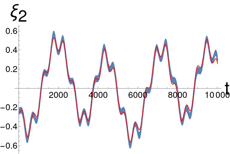
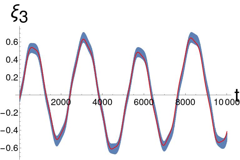
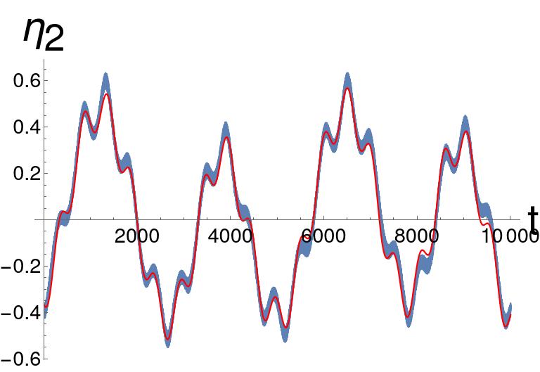
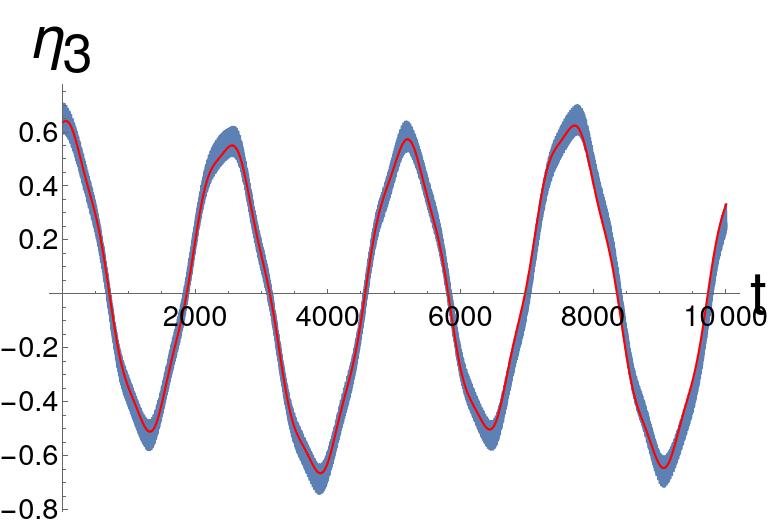
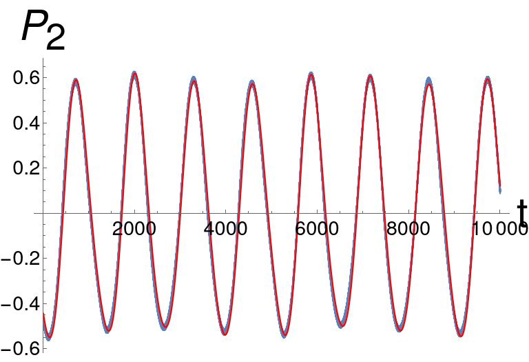
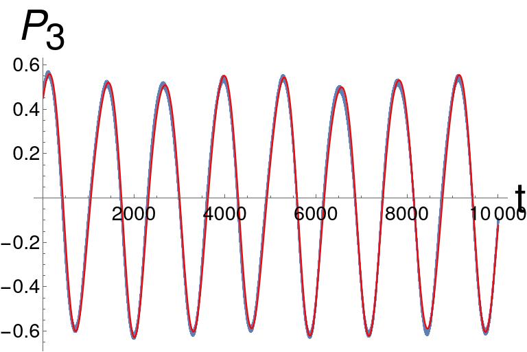
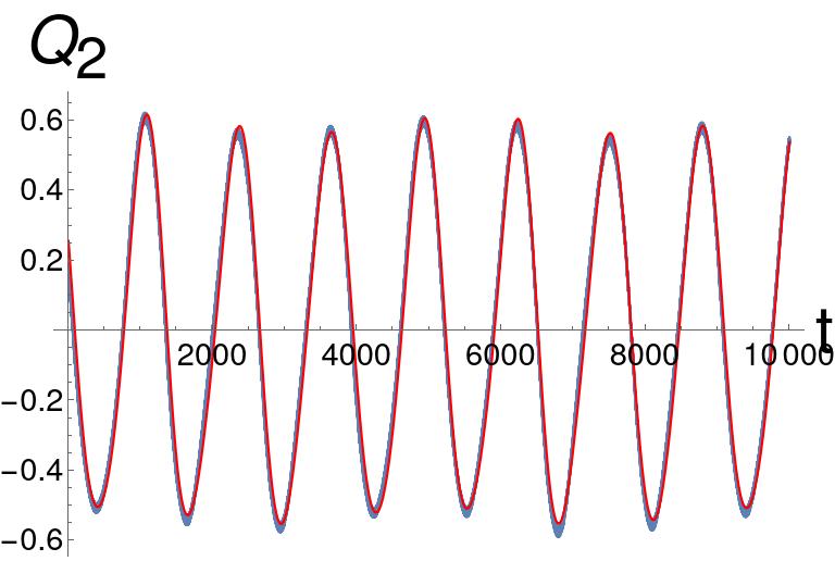
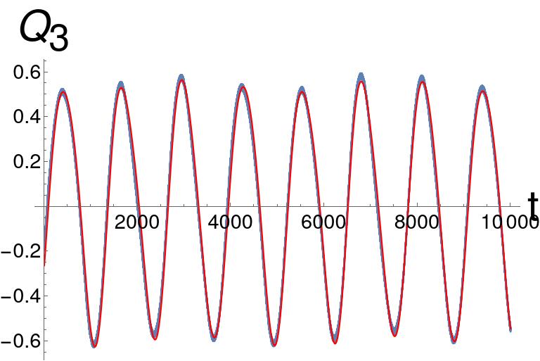
Figure 1: Dynamical behavior of the variables $\xi_{2}$, $\xi_{3}$, $\eta_{2}$, $\eta_{3}$, $P_{2}$, $P_{3}$, $Q_{2}$, $Q_{3}$ (their definition is reported in (2)) as it is computed by numerical integration of the complete (non secular) three-body problem and by the quasi-periodic approximation provided by the FA; the corresponding plots are in blue and red, respectively.

3 The secular quasi-periodic restricted (SQPR) Hamiltonian

Having preassigned the motion of the two outer planets $\upsilon$-And $\mathbf{c}$ and $\upsilon$-And $\mathbf{d}\,$, it is now possible to properly define the secular model for a quasi-periodic restricted four-body problem (hereafter, $4$BP). We start from the Hamiltonian of the $4$BP, given by

$$\mathcal{H}_{4BP}=\sum_{j=1}^{3}\left(\frac{{\bm{p}}_{j}\cdot{\bm{p}}_{j}}{2\,\beta_{j}}-\frac{\mathcal{G}\,m_{0}\,m_{j}}{r_{j}}\right)+\sum_{1\leq i<j\leq 3}\frac{{\bm{p}_{i}}\cdot{\bm{p}_{j}}}{m_{0}}-\sum_{1\leq i<j\leq 3}\frac{\mathcal{G}\,m_{i}\,m_{j}}{|{\bm{r}_{i}}-{\bm{r}_{j}}|}\,.$$ (9)

We recall that the so called secular model of order one in the masses is given by averaging with respect to the mean motion angles, i.e.,

$$\mathcal{H}_{sec}({\bm{\xi}},{\bm{\eta}},{\bm{P}},{\bm{Q}})=\>\int_{\mathbb{T}^{3}}\!\!\!\!\frac{\mathcal{H}_{4BP}({\bm{\Lambda}},{\bm{\lambda}},{\bm{\xi}},{\bm{\eta}},{\bm{P}},{\bm{Q}})}{8\pi^{3}}\,d\lambda_{1}d\lambda_{2}d\lambda_{3}\,.$$ (10)

In the l.h.s. of the equation above, we disregard the dependence on the actions ${\bm{\Lambda}}$, because in the secular approximation of order one in the masses their values $\Lambda_{j}=\beta_{j}\sqrt{\mu_{j}\,a_{j}}\,$, $j=1,2,3$, are constant. Due to the d’Alembert rules (see, e.g., [26] and [25]), it is well known that the secular Hamiltonian can be expanded in the following way:

$$\mathcal{H}_{sec}({\bm{\xi}},{\bm{\eta}},{\bm{P}},{\bm{Q}})=\sum_{s=0}^{\mathcal{N}/2}\sum_{\begin{subarray}{c}|{\bm{i}}|+|{\bm{l}}|+\quad\,\>\>\\ |{\bm{m}}|+|{\bm{n}}|=2s\end{subarray}}\!\!\!\!\!\!c_{{\bm{i}},{\bm{l}},{\bm{m}},{\bm{n}}}\prod_{j=1}^{3}\xi_{j}^{i_{j}}\eta_{j}^{l_{j}}P_{j}^{m_{j}}Q_{j}^{n_{j}}\,,$$ (11)

where $\mathcal{N}$ is the order of truncation in powers of eccentricity and inclination. We fix $\mathcal{N}=8$ in all our computations.

Since we aim at describing the dynamical secular evolution of the innermost planet $\upsilon$-And $\mathbf{b}\,$, it is sufficient to consider the interactions between the two pairs $\upsilon$-And $\mathbf{b}$, $\upsilon$-And $\mathbf{c}$ and $\upsilon$-And $\mathbf{b}$, $\upsilon$-And $\mathbf{d}$. In more details, let $\mathcal{H}_{sec}^{\mathfrak{i}-\mathfrak{j}}$ be the secular Hamiltonian derived from the three-body problem for the planets $\mathfrak{i}$ and $\mathfrak{j}$, averaging with respect to the mean longitudes $\lambda_{\mathfrak{i}}\,$, $\lambda_{\mathfrak{j}}\,$. Its expansion writes as

$$\mathcal{H}^{\mathfrak{i}-\mathfrak{j}}_{sec}(\xi_{\mathfrak{i}},\eta_{\mathfrak{i}},P_{\mathfrak{i}},Q_{\mathfrak{i}},\xi_{\mathfrak{j}},\eta_{\mathfrak{j}},P_{\mathfrak{j}},Q_{\mathfrak{j}})=\sum_{s=0}^{\mathcal{N}/2}\sum_{\begin{subarray}{c}|{\bm{i}}|+|{\bm{l}}|+\quad\,\>\>\\ |{\bm{m}}|+|{\bm{n}}|=2s\end{subarray}}\!\!\!\!\!\!c_{{\bm{i}},{\bm{l}},{\bm{m}},{\bm{n}}}\prod_{j=\mathfrak{i},\mathfrak{j}}\xi_{j}^{i_{j}}\eta_{j}^{l_{j}}P_{j}^{m_{j}}Q_{j}^{n_{j}}\,.$$ (12)

Therefore, a restricted non-autonomous model which approximates the secular dynamics of $\upsilon$-And $\mathbf{b}$ can be defined by considering the terms

$$\mathcal{H}^{1-2}_{sec}(\xi_{1},\eta_{1},P_{1},Q_{1},\xi_{2}(t),\eta_{2}(t),P_{2}(t),Q_{2}(t))+\mathcal{H}^{1-3}_{sec}(\xi_{1},\eta_{1},P_{1},Q_{1},\xi_{3}(t),\eta_{3}(t),P_{3}(t),Q_{3}(t))$$

where $\xi_{2}(t)$, $\eta_{2}(t)$, …$P_{3}(t)$, $Q_{3}(t)$ are replaced with the corresponding quasi-periodic approximations written in both the r.h.s. appearing in formula (6). Let us stress that, having prescribed the motion of the two outermost planets $\upsilon$-And $\mathbf{c}$ and $\upsilon$-And $\mathbf{d}\,$, at this stage the Hamiltonian $\mathcal{H}_{sec}^{2-3}$ does not need to be reconsidered; indeed, it would introduce additional terms that disappear in the equations of motion (see formula (15) which is written below).

We can finally introduce the quasi-periodic restricted Hamiltonian model for the secular dynamics of $\upsilon$-And $\mathbf{b}\,$; it is given by the following $2+3/2$ degrees of freedom Hamiltonian:

$$\mathcal{H}_{sec,\,2+\frac{3}{2}}({\bm{p}},{\bm{q}},\xi_{1},\eta_{1},P_{1},Q_{1}) =\omega_{3}\,p_{3}+\omega_{4}\,p_{4}+\omega_{5}\,p_{5}$$ (13)

$$\phantom{=}+\mathcal{H}^{1-2}_{sec}(\xi_{1},\eta_{1},P_{1},Q_{1},\xi_{2}({\bm{q}}),\eta_{2}({\bm{q}}),P_{2}({\bm{q}}),Q_{2}({\bm{q}}))$$

$$\phantom{=}+\mathcal{H}^{1-3}_{sec}(\xi_{1},\eta_{1},P_{1},Q_{1},\xi_{3}({\bm{q}}),\eta_{3}({\bm{q}}),P_{3}({\bm{q}}),Q_{3}({\bm{q}}))\,,$$

where the pairs of canonical coordinates referring to the planets $\upsilon$-And $\mathbf{c}$ and $\upsilon$-And $\mathbf{d}$ (that are $\xi_{2}\,$, $\eta_{2}\,$, …$P_{3}\,$, $Q_{3}$) are replaced by the corresponding finite Fourier decomposition written in formula (6) as a function of the angles ${\bm{\theta}}$, renamed as ${\bm{q}}$, i.e.,

$${\bm{q}}=(q_{3}\,,\,q_{4}\,,\,q_{5}):=(\theta_{3}\,,\,\theta_{4}\,,\,\theta_{5})={\bm{\theta}}\,.$$ (14)

Let us focus on the summands appearing in the first row of (13), i.e., the Hamiltonian term ${\bm{\omega}}\cdot{\bm{p}}\,$, where ${\bm{\omega}}$ is the fundamental angular velocity vector (defined in formula (LABEL:freq.fond.CD)) and ${\bm{p}}=(p_{3},p_{4},p_{5})$ is made by three so called “dummy variables”, which are conjugated to the angles ${\bm{q}}$. The role they play is made clear by the equations of motion for the innermost planet, which write in the following way in the framework of the restricted quasi-periodic secular approximation:

$$\begin{cases}\dot{q_{3}}=\partial\mathcal{H}_{sec,\,2+\frac{3}{2}}/\partial p_{3}=\omega_{3}\\ \dot{q_{4}}=\partial\mathcal{H}_{sec,\,2+\frac{3}{2}}/\partial p_{4}=\omega_{4}\\ \dot{q_{5}}=\partial\mathcal{H}_{sec,\,2+\frac{3}{2}}/\partial p_{5}=\omega_{5}\\ \dot{\xi}_{1}=-\partial\mathcal{H}_{sec,\,2+\frac{3}{2}}/\partial\eta_{1}=-\partial\big{(}\mathcal{H}^{1-2}_{sec}+\mathcal{H}^{1-3}_{sec}\big{)}/\partial\eta_{1}\\ \dot{\eta}_{1}=\partial\mathcal{H}_{sec,\,2+\frac{3}{2}}/\partial\xi_{1}=\partial\big{(}\mathcal{H}^{1-2}_{sec}+\mathcal{H}^{1-3}_{sec}\big{)}/\partial\xi_{1}\\ \dot{P}_{1}=-\partial\mathcal{H}_{sec,\,2+\frac{3}{2}}/\partial Q_{1}=-\partial\big{(}\mathcal{H}^{1-2}_{sec}+\mathcal{H}^{1-3}_{sec}\big{)}/\partial Q_{1}\\ \dot{Q}_{1}=\partial\mathcal{H}_{sec,\,2+\frac{3}{2}}/\partial P_{1}=\partial\big{(}\mathcal{H}^{1-2}_{sec}+\mathcal{H}^{1-3}_{sec}\big{)}/\partial P_{1}\end{cases}\,.$$ (15)

Due to the occurrence of the term ${\bm{\omega}}\cdot{\bm{p}}$ in the Hamiltonian $\mathcal{H}_{sec,\,2+\frac{3}{2}}\,$, the first three equations admit ${\bm{q}}(t)={\bm{\omega}}t$ as a solution, in agreement with formulæ (7) and (14). This allows to reinject the wanted quasi-periodic time-dependence in the Fourier approximations $\xi_{2}({\bm{q}})$, $\eta_{2}({\bm{q}})$, $\ldots$ $P_{3}({\bm{q}})$, $Q_{3}({\bm{q}})$. As a matter of fact, we do not need to compute the evolution of $({p}_{3}(t),{p}_{4}(t),{p}_{5}(t))$ because they do not exert any influence on the motion of $\upsilon$-And $\mathbf{b}\,$; they are needed just if one is interested in checking that the energy is preserved, because it is given by the evaluation of $\mathcal{H}_{sec,\,2+\frac{3}{2}}\,$.

We also recall that, in order to produce a restricted quasi-periodic secular model, it is possible to apply the closed-form averaging, which is compared in [20] with the computational method that is adopted here and is based on the expansions in Laplace coefficients. Finally, we emphasize what is discussed below.

Remark 3.1.

The Hamiltonian $\mathcal{H}_{sec,\,2+\frac{3}{2}}$ is invariant with respect to a particular class of rotations. Thus, it admits a constant of motion that could be reduced, so to decrease by one the number of degrees of freedom of the model.

In order to clarify the statement above, it is convenient to introduce a complete set of action-angle variables, defining two new pairs of canonical coordinates $\xi_{1}=\sqrt{2\Gamma_{1}}\cos(\varpi_{1})$, $\eta_{1}=\sqrt{2\Gamma_{1}}\sin(-\varpi_{1})$, $P_{1}=\sqrt{2\Theta_{1}}\cos(\Omega_{1})$, $Q_{1}=\sqrt{2\Theta_{1}}\sin(-\Omega_{1})$, referring to a pair of orbital angles of $\upsilon$-And $\mathbf{b}$, i.e., $\varpi_{1}$ and $\Omega_{1}\,$, that are the longitudes of the pericenter and of the node, respectively (see definition (2) of the Poincaré canonical variables). Thus, it is possible to verify the following invariance law:

$${-\frac{\partial\,\mathcal{H}_{sec,\,2+\frac{3}{2}}}{\partial\xi_{1}}\,\,\frac{\partial\,\xi_{1}}{\partial\varpi_{1}}-\frac{\partial\,\mathcal{H}_{sec,\,2+\frac{3}{2}}}{\partial\eta_{1}}\,\frac{\partial\,\eta_{1}}{\partial\varpi_{1}}-\frac{\partial\,\mathcal{H}_{sec,\,2+\frac{3}{2}}}{\partial P_{1}}\,\frac{\partial P_{1}}{\partial\Omega_{1}}-\frac{\partial\,\mathcal{H}_{sec,\,2+\frac{3}{2}}}{\partial Q_{1}}\,\frac{\partial Q_{1}}{\partial\Omega_{1}}}$$

Therefore, $p_{3}+p_{4}+p_{5}+\Gamma_{1}+\Theta_{1}$ is preserved; such a quantity, apart from an inessential additional constant, is equivalent to the total angular momentum.

The above invariance law is better understood, recalling that $q_{3}$ and $q_{4}$ correspond to the longitudes of the pericenters of $\upsilon$-And $\mathbf{c}$ and $\upsilon$-And $\mathbf{d}$, respectively, while $q_{5}$ refers to the longitude of the nodes of $\upsilon$-And $\mathbf{c}$ and $\upsilon$-And $\mathbf{d}$ (that in the Laplace frame, determined by taking into account only these two exoplanets, are opposite one to the other). This identification is due to the way we have determined $(q_{3},q_{4},q_{5})$ by decomposing some specific signals of the secular dynamics of the outer exoplanets (this is made by using the Frequency Analysis, as it is explained in Section 2). Thus, the aforementioned invariance law is due to the fact that the dynamics of the model we are studying does depend just on the pericenters arguments of the three exoplanets and on the difference between the longitude of the nodes of $\upsilon$-And $\mathbf{b}$ and $\upsilon$-And $\mathbf{c}$, i.e., $\Omega_{1}-\Omega_{2}=\Omega_{1}-\Omega_{3}-\pi$. Therefore, the Hamiltonian is invariant with respect to any rotation of the same angle that is applied to all the longitudes of the nodes; as it is well known, by Noether theorem, this is equivalent to the preservation of the total angular momentum.

3.1 Numerical validation of the SQPR model

In order to validate our secular quasi-periodic restricted (hereafter SQPR) model describing the dynamics of $\upsilon$-And $\mathbf{b}$, we want to compare the numerical integrations of the complete 4BP with the ones of the equations of motion (15). Let us recall that the chosen values of parameters and initial conditions for the two outer planets are given in Table 1. For what concerns the orbital elements of the innermost planet $\upsilon$-And $\mathbf{b}$, both the inclination $\mathrm{i}_{1}$ and the longitude of the ascending node $\Omega_{1}$ are unknown (see, e.g., [22]). The available data for $\upsilon$-And $\mathbf{b}$ are reported in Table 7. Among the possible values of the initial orbital parameters of $\upsilon$-And $\mathbf{b}$, we have chosen $a_{1}\,$, $\mathrm{e}_{1}$, $M_{1}$ and $\omega_{1}$ as in the stable prograde trial PRO2 described in [5]. They are reported in Table 7 and are compatible with the available ranges of values appearing in Table 7. Let us recall that the dynamical evolution of the SQPR model does not depend on the mass of $\upsilon$-And $\mathbf{b}$, therefore, the choice about its value is not reported in Table 7. For what concerns the unknown initial values of the inclination and of the longitude of nodes, we have decided to vary them so as to cover a $2$D regular grid of values $(\mathrm{i}_{1}(0),\,\Omega_{1}(0))\in I_{\mathrm{i}}\times I_{\Omega}=[6.865^{\circ},34^{\circ}]\times[0^{\circ},360^{\circ}]$, dividing $I_{\mathrm{i}}$ and $I_{\Omega}$, respectively, in $20$ and $60$ sub-intervals; this means that the widths of the grid-steps are equal to $1.35675^{\circ}$ and $6^{\circ}$ in inclination and longitude of nodes, respectively. Let us recall that the lowest possible value of the interval $I_{\mathrm{i}}$, i.e. $\mathrm{i}_{2}(0)=6.865^{\circ}$, corresponds to the inclination of $\upsilon$-And $\mathbf{c}$. Considering values smaller than $\mathrm{i}_{2}(0)$ could be incoherent with the assumptions leading to the SPQR model we have just introduced; indeed, the factor $1/\sin(\mathrm{i}_{1}(0))$ increases the mass of the exoplanet by one order of magnitude with respect to the minimal one. Therefore, for small values of $\mathrm{i}_{1}(0)$ the mass of $\upsilon$-And $\mathbf{b}$ could become so large that the effects exerted by its gravitational attraction on the outer exoplanets could not be neglected anymore. On the other hand, it will be shown in the sequel that the stability region for the orbital motion of $\upsilon$-And $\mathbf{b}$ nearly completely disappears for values of $\mathrm{i}_{1}(0)$ larger than $34^{\circ}$. These are the reasons behind our choice about the lower and upper limits of $I_{\mathrm{i}}$.

	$\upsilon$-And $\bf{b}$
$m\,\sin(\mathrm{i})\,[M_{J}]$	$0.69\pm 0.016$
$a(0)\,[AU]$	$0.0594\pm 0.0003$
$\mathrm{e}(0)$	$0.012\pm 0.005$
$\omega(0)\,[^{\circ}]$	$44.106\pm 25.561$

Table 6: Available data for the orbital parameters of the exoplanet $\upsilon$-And $\mathbf{b}$. The values above are reported from Table $13$ of [22].

	$\upsilon$-And $\bf{b}$
$a(0)\,[AU]$	$0.0594$
$\mathrm{e}(0)$	$0.011769$
$M(0)\,[^{\circ}]$	$103.53$
$\omega(0)\,[^{\circ}]$	$51.14$

Table 7: Values of the initial orbital parameters for $\upsilon$-And $\mathbf{b}$ as they have been selected in the stable prograde trial PRO2 of [5] (Table $3\,$).

We emphasize that the study of the stability domain, as it is deduced by the numerical integrations, can help us to obtain information about the possible ranges of the unknown values $(\mathrm{i}_{1}(0),\Omega_{1}(0))$. Moreover, the comparisons between the numerical integrations of the complete $4$BP and the ones of the SQPR model aim to demonstrate that the agreement is sufficiently good so that it becomes possible to directly work with the latter Hamiltonian model, that has to be considered easier than the former, because the degrees of freedom are $2+3/2$ instead of $9$.

3.1.1 Numerical integration of the complete $4$-body problem

For each pair of values $(\mathrm{i}_{1}(0)\,,\Omega_{1}(0))\in I_{\mathrm{i}}\times I_{\Omega}$ ranging in the $20\times 60$ regular grid we have previously prescribed, we first compute the corresponding initial orbital elements of the three exoplanets in the Laplace-reference frame, then we perform the numerical integration of the complete 4BP Hamiltonian (9) by using the symplectic method of type $\mathcal{SBAB}_{3}\,$. Contrary to the SPQR model, the numerical integrations of the 4BP are affected by the mass of $\upsilon$-And $\mathbf{b}$; its value is simply fixed in such a way that $m_{1}=0.674/\sin(\mathrm{i}_{1}(0))\,$.

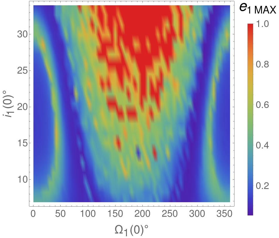
(a)

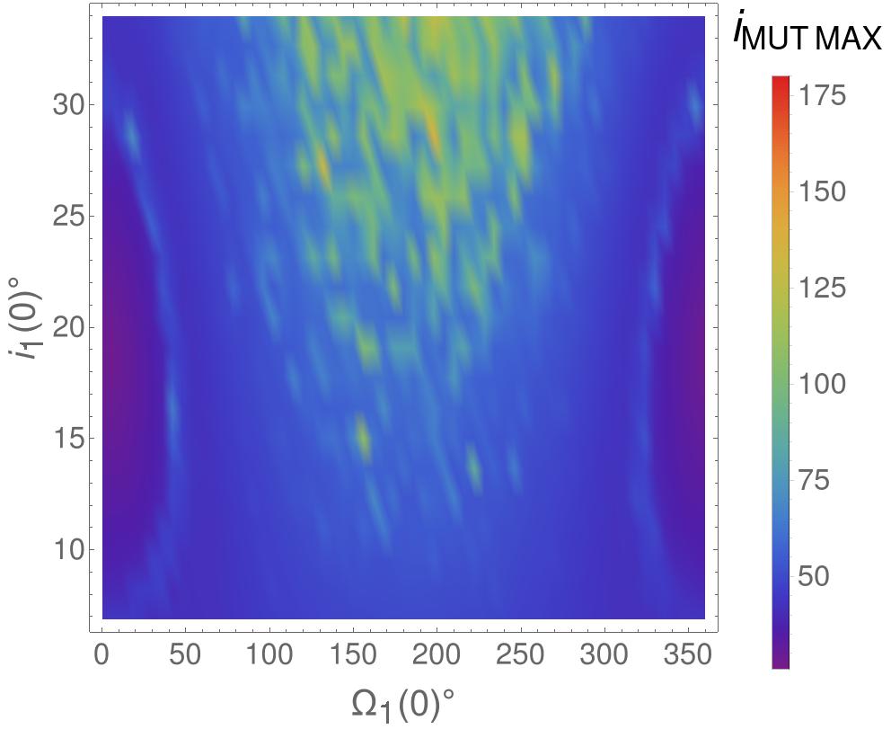
(b)

Figure 2: Color-grid plots of the maximal value reached by the eccentricity of $\upsilon$-And $\mathbf{b}$ (on the left) and by the mutual inclination between $\upsilon$-And $\mathbf{b}$ and $\upsilon$-And $\mathbf{c}$ (on the right). The maxima are computed during the symplectic numerical integrations of the 4BP which cover a timespan of $10^{5}$ yr.

The largest value reached by the eccentricity can be considered as a very simple numerical indicator about the stability of the orbital configurations. The maximum eccentricity obtained along each of the $21\times 60$ numerical integrations is reported in the left panel of Figure 2. In particular, since we are interested in initial conditions leading to regular behavior, i.e., avoiding quasi-collisions, every time that the eccentricity $\mathrm{e}_{1}$ exceeds a threshold value (fixed to be equal to $0.85$), in the color-grid plots its maximal value is arbitrarily set equal to one. Moreover, since we expect that $\upsilon$-And $\mathbf{c}$ is the most massive planet in that extrasolar system and being it the closest one to $\upsilon$-And $\mathbf{b}$, it is natural to focus the attention also on the mutual inclination between $\upsilon$-And $\mathbf{b}$ and $\upsilon$-And $\mathbf{c}\,$. Let us recall that it is defined in such a way that

$$\cos(\mathrm{i}_{{mut}_{\mathbf{b}\mathbf{c}}})=\cos(\mathrm{i}_{1})\cos(\mathrm{i}_{2})+\sin(\mathrm{i}_{1})\sin(\mathrm{i}_{2})\cos(\Omega_{1}-\Omega_{2})\,;$$ (16)

therefore, for each numerical integration it is also possible to compute the maximal value reached by $\mathrm{i}_{{mut}_{\mathbf{b}\mathbf{c}}}\,$. The results are reported in the right panel of Figure 2. In both those panels the color-grid plots are provided as functions of the initial values of the longitude of nodes $\Omega_{1}$ and the inclination $\mathrm{i}_{1}\,$, which are reported on the $x$ and $y$ axes, respectively. By comparing the two plots in the Figure panels 2a and 2b, one can easily appreciate that the regions which have to be considered as dynamically unstable, because the eccentricity of $\mathrm{e}_{1}$ can grow to large values, correspond also to large mutual inclinations of the planetary orbits of $\upsilon$-And $\mathbf{b}$ and $\upsilon$-And $\mathbf{c}$.

We remark that the value of the initial mean anomaly $M_{1}(0)$ is missing among the available observational data reported in Table 7. As a matter of fact, mean anomalies of exoplanets are in general so poorly known that usually their values are not reported in the public databases. However, in order to understand if (and up to what extent) the initial value $M_{1}(0)$ can affect the dynamics of $\upsilon$-And $\mathbf{b}\,$, we repeat all the numerical integrations of the $4$BP for four different initial values of $M_{1}\,$, chosen so as to have one of them belonging to each of the quadrants $[0^{\circ},90^{\circ}]\,$, $[90^{\circ},180^{\circ}]\,$, $[180^{\circ},270^{\circ}]\,$ and $[270^{\circ},360^{\circ}]\,$. In Figure 3 we report three examples; in particular, they show the color-grid plots of the maximal value reached by the eccentricity $\mathrm{e}_{1}\,$, taking $M_{1}(0)$ as $360^{\circ}/7=51.4286^{\circ}$, $4\cdot 360^{\circ}/7=205.714^{\circ}$ and $6\cdot 360^{\circ}/7=308.571^{\circ}$, respectively. For what concerns the region $[90^{\circ},180^{\circ}]$, let us recall that Figure 2a refers to $M_{1}(0)=103.53^{\circ}$. The comparison between Figures 2a and 3 shows that the choice of the value of $M_{1}(0)$ does not seem to produce any remarkable impact on the global structure of the dinamical stability of these exoplanetary orbits.

Figure 3: Color-grid plots of the maximal value reached by the eccentricity of $\upsilon$-And $\mathbf{b}$. The maxima are computed during the symplectic numerical integrations of the 4BP which cover a timespan of $10^{5}$ yr. The results are obtained by numerical integrations which refer to sets of initial conditions that differ (passing from one panel to another) just because of the choice of the initial values of the mean anomaly; from left to right the plots refer to $M_{1}(0)$ equal to $51.4286^{\circ}$, $205.714^{\circ}$, and $308.571^{\circ}$, respectively.

Moreover, the same conclusion applies also to the increasing factor $1/\sin(\mathrm{i}_{1}(0))$ (with $\mathrm{i}_{1}(0)\in I_{\mathrm{i}}$) which multiplies the minimal mass of $\upsilon$-And $\mathbf{b}\,$ in such a way to determine the value of $m_{1}\,$. In fact, substantial differences are not observed between Figures 2 and 4.

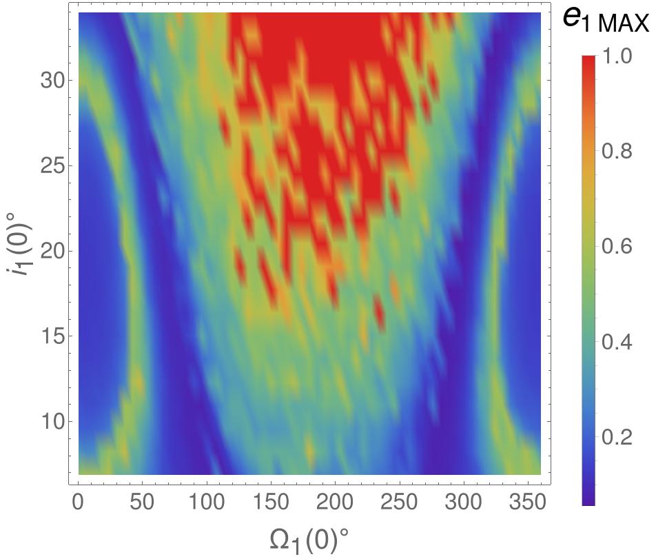
(a)

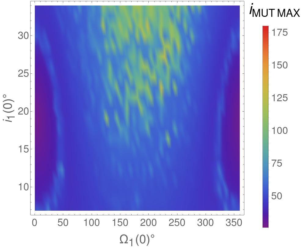
(b)

Figure 4: Color-grid plots of the maximal value reached by the eccentricity of $\upsilon$-And $\mathbf{b}$ (on the left) and by the mutual inclination between $\upsilon$-And $\mathbf{b}$ and $\upsilon$-And $\mathbf{c}$ (on the right). The maxima are computed during the symplectic numerical integrations of the 4BP which cover a timespan of $10^{5}$ yr. As the only difference with respect to the numerical integration whose results are reported in Figure 2, here the mass of $\upsilon$-And $\mathbf{b}$ is always kept fixed so as to be equal to its minimal value $m_{1}=0.674\,$.

3.1.2 Numerical integration of the secular quasi-periodic restricted model

We want now to compare the previous results with those found in the SQPR approximation of the $4$-body problem, performing numerical integrations of the system of equations (15). In order to make these comparisons coherent, also here we consider the data listed in Table 7 as initial conditions for the orbital elements of $\upsilon$-And $\mathbf{b}$ which are completed with the values of $(\mathrm{i}_{1}(0)\,,\Omega_{1}(0))$ ranging in the $20\times 60$ regular grid that covers $I_{\mathrm{i}}\times I_{\Omega}=[6.865^{\circ},34^{\circ}]\times[0^{\circ},360^{\circ}]$. At the beginning of the computational procedure, the initial values of the orbital elements are determined in the Laplace reference frame, which is fixed by taking into account only the two outermost planets (i.e., the total angular momentum of the system is given only by the sum of the angular momentum of $\upsilon$-And $\mathbf{c}$ and $\upsilon$-And $\mathbf{d}\,$). Of course, this is made in agreement with our choice to consider a restricted framework, because we are assuming that the mass of $\upsilon$-And $\mathbf{b}$ is so small that can be neglected.

For each numerical integration we compute the maximal value reached by the eccentricity $\mathrm{e}_{1}$ and the mutual inclination $\mathrm{i}_{{mut}_{\mathbf{b}\mathbf{c}}}\,$. The results are reported in the color-grid plots of the left and right panels of Figure 5, respectively. Once again, they are provided as functions of $\Omega_{1}(0)$ and $\mathrm{i}_{1}(0)\,$, whose values appear on the $x$ and $y$ axes, respectively.

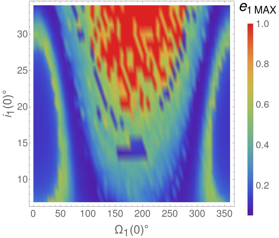
(a)

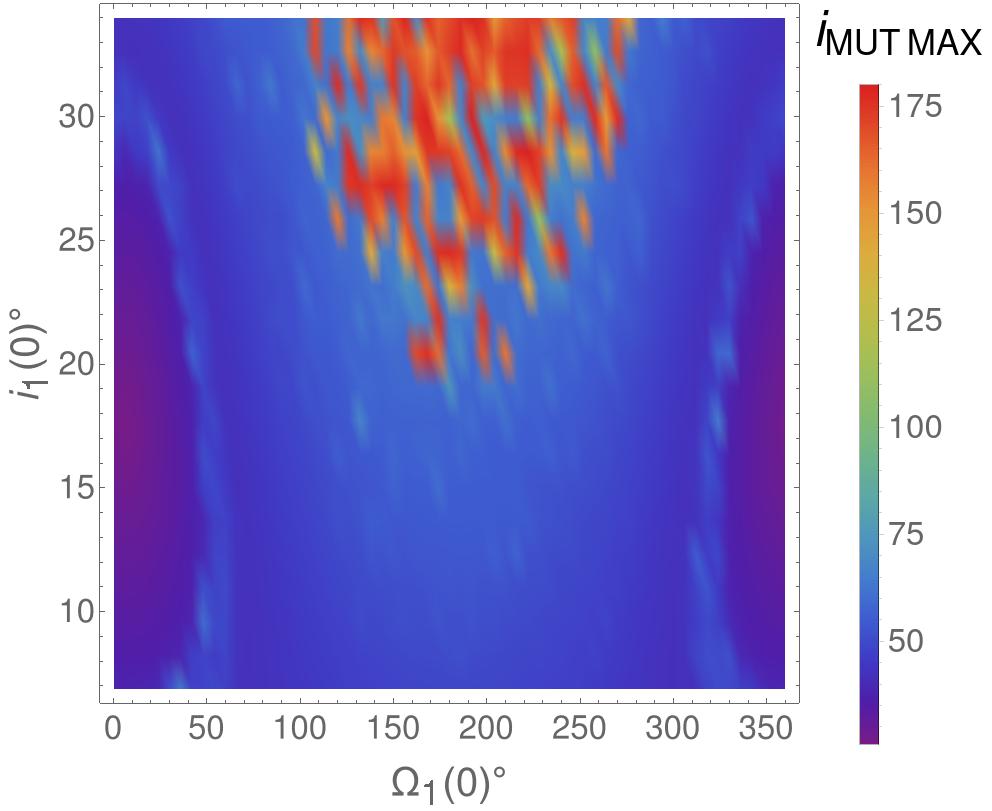
(b)

Figure 5: Color-grid plots of the maximal value reached by the eccentricity of $\upsilon$-And $\mathbf{b}$ (on the left) and by the mutual inclination between $\upsilon$-And $\mathbf{b}$ and $\upsilon$-And $\mathbf{c}$ (on the right). The maxima are computed along the RK4 numerical integrations of the equations of motion (15) of the SQPR model, covering a timespan of $10^{5}$ yr.

Comparing Figures 2a with 5a and 2b with 5b, respectively, we can immediately conclude the striking similarity of the color-grid plots, implying the same dependence of the dynamics on the initial values of the orbital elements $\mathrm{i}_{1}(0)$ and $\Omega_{1}(0)\,$ in either model. In particular, the regions of stability located at the two lateral sides of the plots, where the orbit of $\upsilon$-And $\mathbf{b}$ does not become very eccentric, are identical. This occurs also for what concerns the plots of the maximal mutual inclination. However, some discrepancies are evident in the central parts of the panels, i.e. for values of $\Omega_{1}(0)$ ranging between $90^{\circ}$ and $270^{\circ}$. We stress that this lack of agreement between the results provided by the two models is expected in these central regions of the panels. Indeed, let us recall that the SQPR model has been introduced starting from some classical expansions in powers of eccentricities and inclinations. Therefore, it is reasonable to expect a deterioration of the accuracy of the SQPR model in the orbital dynamics depicted in the central regions of the plots where large values of the eccentricity $\mathrm{e}_{1}$ and the mutual inclination are attained. We emphasize that similar remarks about the very strong impact of the initial value $\Omega_{1}(0)$ on the orbital stability of $\upsilon$-And $\mathbf{b}$ can be found in Section 4.2 of [27].

A further exploration of the stable and chaotic regions of Figure 5a can be done by applying the so called Frequency Map Analysis method (see, e.g., [13]), in order to study the signal $\xi_{1}(t)+i\eta_{1}(t)$ produced by the numerical integration of the system (15), i.e., in the SQPR approximation. We perform the numerical integrations as prescribed at the beginning of the present Section, taking into account only a few values in $I_{\mathrm{i}}\,$ for the initial inclinations, i.e., $\mathrm{i}_{1}(0)=6.865^{\circ},\,8.22175^{\circ},\,9.5785^{\circ},\,10.9353^{\circ}$ and $\Omega_{1}(0)\in I_{\Omega}\,$. In Figure 6 we report the behaviour of the angular velocity corresponding to the first component of the approximation of $\xi_{1}(t)+i\eta_{1}(t)$, as obtained by applying the FA computational algorithm; therefore, this quantity is related to the precession rate of $\varpi_{1}\,$. As initial value for the inclination $\mathrm{i}_{1}(0)$ we fix $6.865^{\circ}$ for Figure 6a and $10.9353^{\circ}$ for Figure 6b. We do not report the cases $(\mathrm{i}_{1}(0),\Omega_{1}(0))\in\{8.22175^{\circ},\,9.5785^{\circ}\}\times I_{\Omega}\,$, since the behaviour of those plots is similar to the ones in Figure 6.

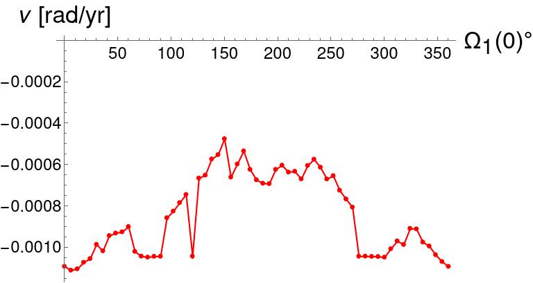
(a)

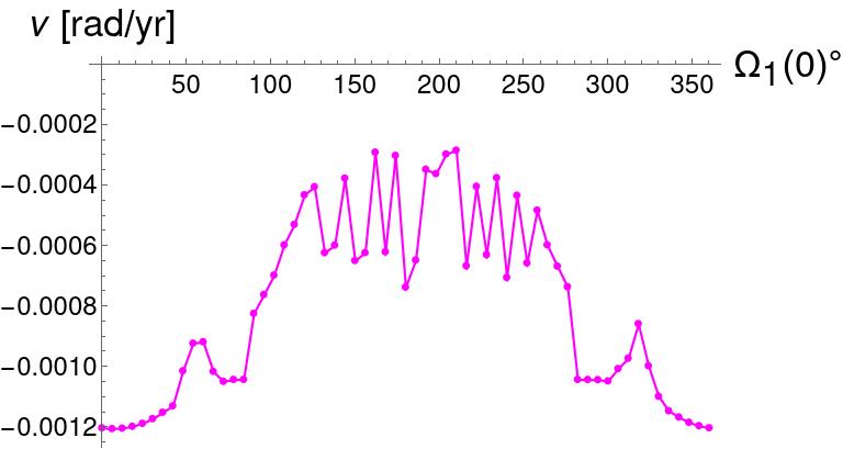
(b)

Figure 6: Behaviour of the fundamental angular velocity $\nu$ as obtained by applying the Frequency Map Analysis method to the signal $\xi_{1}(t)+i\eta_{1}(t)\,$, computed through the RK4 numerical integration of the SQPR model (15), covering a timespan of $1.31072\cdot 10^{5}$ yr. We take, as initial conditions, $(\mathrm{i}_{1}(0),\Omega_{1}(0))\in\{6.865^{\circ}\}\times I_{\Omega}$ for the left panel and $(\mathrm{i}_{1}(0),\Omega_{1}(0))\in\{10.9353^{\circ}\}\times I_{\Omega}$ for the right one.

The situation is well described in Figure 6b and analogous considerations can be done for Figure 6a. For what concerns the values of $\Omega_{1}(0)$ in the range $[0,\sim 50^{\circ}]$ and $[\sim 325^{\circ},\,360^{\circ}]$ we can observe a regular behaviour of the angular velocity $\nu$ which is also monotone with the only exception of the local minimum. According to the interpretation of the Frequency Map Analysis (in the light of KAM theory), such a regular regime is due to the presence of many invariant tori which fill the stability region located at the two lateral sides of the plot 5a. Instead for values of $\Omega_{1}(0)$ in $[\sim 50^{\circ},\sim 70^{\circ}]\cup[\sim 300^{\circ},\,\sim 325^{\circ}]$ and $\Omega_{1}(0)$ in $[\sim 120^{\circ},\,\sim 270^{\circ}]$ we observe a strongly irregular behaviour, which corresponds to the lateral green stripes and the internal green region of Figure 5a. Thus, they represent chaotic regions in proximity of a secular resonance. Indeed, in Figure 6b the angular velocity is constant for values of $\Omega_{1}(0)$ in $[\sim 70^{\circ},\,\sim 85^{\circ}]$ and $[\sim 280^{\circ},\,\sim 300^{\circ}]$ (corresponding to part of the blue central stripes of Figure 5a). More precisely, the value of $\nu$ is equal to $\simeq-1.04\cdot 10^{-3}\,$, that is $\omega_{4}\,$, i.e., one of the fundamental angular velocities which characterize the quasi-periodic motion of the outer planets (see Eq. (LABEL:freq.fond.CD)). This allows us to conclude that they represent the stable central part of a resonant region.

4 Introduction of a secular model by a normal form approach

This Section aims at manipulating the Hamiltonian with normal form algorithms in order to define a new model that is more compact; this allows us to simulate the secular dynamics of $\upsilon$-And $\mathbf{b}$ with much faster numerical integrations. In fact, we describe a reduction of the number of degrees of freedom (DOF) of our Hamiltonian model. For such a purpose, we apply two normal form methods: first, we perform the construction of an elliptic torus, hence, we proceed removing the angles ($q_{3},q_{4},q_{5}\,$) whose evolution is linearly depending on time. The latter elimination is made by applying a normalization method à la Birkhoff in such a way to introduce a so called resonant normal form that includes, at least partially, the long-term effects due to the outer planets motion.

4.1 Normal form algorithm constructing elliptic tori

In [9] the existence of invariant elliptic tori in 3D planetary problems with $n$ bodies has been proved by using a normal form method which is explicitly constructive. However, such an approach does not look suitable to be directly applied to Hamiltonian secular models, because in this latter case the separation between fast and slow dynamics is lost. Therefore, we follow the explanatory notes [17], where the algorithm constructing the normal form for elliptic tori is compared with the classical one à la Kolmogorov, which is at the basis of the original proof scheme of the KAM theorem. We first summarize this general procedure leading to the construction of elliptic tori. We then add some comments explaining how this general method can be suitably adapted to our problem.

We start considering a Hamiltonian $\mathcal{H}^{(0)}$ written as follows:

$$\mathcal{H}^{(0)}({\bm{p}},{\bm{q}},{\bm{I}},{\bm{\alpha}}) =\mathcal{E}^{(0)}+{\bm{\omega}}^{(0)}\cdot{\bm{p}}+{\bm{\Omega}}^{(0)}\cdot{\bm{I}}+\sum_{s\geq 0}\sum_{l\geq 3}f_{l}^{(0,s)}({\bm{p}},{\bm{q}},{\bm{I}},{\bm{\alpha}})$$ (17)

$$\phantom{=}+\sum_{s\geq 1}f_{0}^{(0,s)}({\bm{q}})+\sum_{s\geq 1}f_{1}^{(0,s)}({\bm{q}},{\bm{I}},{\bm{\alpha}})+\sum_{s\geq 1}f_{2}^{(0,s)}({\bm{p}},{\bm{q}},{\bm{I}},{\bm{\alpha}})\,,$$

where $\mathcal{E}^{(0)}$ is a constant term, representing the energy, $({\bm{p}},{\bm{q}})\in\mathbb{R}^{n_{1}}\times\mathbb{T}^{n_{1}}\,$, $({\bm{I}},{\bm{\alpha}})\in\mathbb{R}^{n_{2}}_{\geq 0}\times\mathbb{T}^{n_{2}}$ are action-angle variables and $({\bm{\omega}}^{(0)},{\bm{\Omega}}^{(0)})\in\mathbb{R}^{n_{1}}\times\mathbb{R}^{n_{2}}$ is the angular velocity vector. The symbol $f_{l}^{(r,s)}$ is used to denote a function of the variables $({\bm{p}},{\bm{q}},{\bm{I}},{\bm{\alpha}})\,$, such that $l$ is the total degree in the square root of the actions $({\bm{p}}\,,{\bm{I}})$, $s$ is the index such that the maximum trigonometric degree, in the angles $({\bm{q}},{\bm{\alpha}})\,$, is $sK$ (for a fixed positive integer $K$) and $r$ refers to the normalization step. In more details, we can say that $f_{l}^{(0,s)}\!\!\in\mathfrak{P}_{l,sK}\,$, which is a class of functions that we introduce as follows.

Definition 4.1.

We say that $g\in\mathfrak{P}_{l,sK}$ if $\displaystyle{g\in\!\!\!\!\bigcup_{\begin{subarray}{c}\widehat{m}\geq 0,\,\widehat{l}\geq 0\\ 2\widehat{m}+\widehat{l}=l\end{subarray}}\!\!\!\!\widehat{\mathfrak{P}}_{\widehat{m},\widehat{l},sK}\,,}$ where

$$\widehat{\mathfrak{P}}_{\widehat{m},\widehat{l},sK}=\Bigg{\{} g:\mathbb{R}^{n_{1}}\times\mathbb{T}^{n_{1}}\times\mathbb{R}_{\geq 0}^{n_{2}}\times\mathbb{T}^{n_{2}}\to\mathbb{R}\,:$$

$$g({\bm{p}},{\bm{q}},{\bm{I}},{\bm{\alpha}})\!=\!\!\!\!\!\sum_{\begin{subarray}{c}{\bm{m}}\in\mathbb{N}^{n_{1}}\\ |{\bm{m}}|=\widehat{m}\end{subarray}}\sum_{\begin{subarray}{c}{\bm{l}}\in\mathbb{N}^{n_{2}}\\ |{\bm{l}}|=\widehat{l}\end{subarray}}\sum_{\begin{subarray}{c}{\bm{k}}\in\mathbb{Z}^{n_{1}}\\ |{\bm{k}}|+|\widehat{{\bm{l}}}|\leq sK\end{subarray}}\!\!\!\!\!\!\!\!\!\!\!\!\!\!\!\!\sum_{\begin{subarray}{c}\qquad\quad\widehat{l}_{j}=-l_{j},-l_{j}+2,\ldots,l_{j}\\ j=1,\ldots,n_{2}\end{subarray}}\!\!\!\!\!\!\!\!\!\!\!c_{{\bm{m}},{\bm{l}},{\bm{k}},\widehat{{\bm{l}}}}\,\,\,{\bm{p}}^{{\bm{m}}}\left(\sqrt{{\bm{I}}}\right)^{{\bm{l}}}e^{i\left({\bm{k}}\cdot{\bm{q}}+\widehat{{\bm{l}}}\cdot{\bm{\alpha}}\right)}\Bigg{\}}\,.$$

A few remarks about the above definition are in order. First, since we deal with real functions, the complex coefficients must be such that $c_{{\bm{m}},{\bm{l}},-{\bm{k}},-\widehat{{\bm{l}}}}=\bar{c}_{{\bm{m}},{\bm{l}},{\bm{k}},\widehat{{\bm{l}}}}\,$. Moreover, the rules about the integer coefficients vector $\widehat{{\bm{l}}}$ are such that, $\forall\,j=1,\ldots,n_{2}\,$, the $j$-th component of the Fourier harmonic $\widehat{l}_{j}$ (that refers to the angle $\alpha_{j}$) must have the same parity with respect to the corresponding degree $l_{j}$ of $\sqrt{I_{j}}$ and must satisfy the inequality $|\widehat{l}_{j}|\leq l_{j}\,$.

Let us here emphasize that our SQPR model of the secular dynamics of $\upsilon$-And $\mathbf{b}$ can be reformulated in such a way to be described by a Hamiltonian of the type (17); this will be explained in detail at the beginning of Section 5.

The following statement plays a substantial role, since it ensures that the structure of the functions $f_{l}^{(r,s)}$ is preserved while the normalization algorithm is iterated.

Lemma 4.1.

Let us consider two generic functions $g\in\mathfrak{P}_{l,sK}$ and $h\in\mathfrak{P}_{m,rK}\,$, where $K$ is a fixed positive integer number. Then

$$\{g,h\}=L_{h}\,g\,\in\,\mathfrak{P}_{l+m-2,\,(r+s)K}\qquad\forall\,l,\,m,\,r,\,s\,\in\,\mathbb{N}\,,$$

where we trivially extend the definition 4.1 in such a way that $\mathfrak{P}_{-2,\,sK}=\mathfrak{P}_{-1,\,sK}=\{0\}$ $\forall\ s\in\mathbb{N}$.

The algorithm constructing the normal form for elliptic tori is applied to Hamiltonians of the type (17), where the terms appearing in the second row (namely, $\sum_{s\geq 1}\sum_{l=0}^{2}f_{l}^{(0,s)}({\bm{p}},{\bm{q}},{\bm{I}},{\bm{\alpha}})\,$) are considered as the perturbation to remove. Therefore, one can easily realize that such a perturbation must be sufficiently small so that the procedure behaves well as regards convergence. There are general situations where this essential smallness condition is satisfied. For instance, this occurs for Hamiltonian systems in the neighborhood of a stable equilibrium point; in fact, it is possible to prove that, $f_{l}^{(0,s)}=\mathcal{O}(\varepsilon^{s})\,$, where $\varepsilon$ is a small parameter which denotes the first approximation of the distance (expressed in terms of the actions) between the elliptic torus and the stable equilibrium point. The elimination of the small perturbing terms can be done through a sequence of canonical transformations, leading the Hamiltonian in the following final form:

$$\mathcal{H}^{(\infty)}(\tilde{{\bm{p}}},\tilde{{\bm{q}}},\tilde{{\bm{I}}},\tilde{{\bm{\alpha}}}) =\mathcal{E}^{(\infty)}+{\bm{\omega}}^{(\infty)}\cdot\tilde{{\bm{p}}}+{\bm{\Omega}}^{(\infty)}\cdot\tilde{{\bm{I}}}+\sum_{s\geq 0}\sum_{l\geq 3}f_{l}^{(\infty,s)}(\tilde{{\bm{p}}},\tilde{{\bm{q}}},\tilde{{\bm{I}}},\tilde{{\bm{\alpha}}})\,,$$ (18)

with $f_{l}^{(\infty,s)}\in\mathfrak{P}_{l,sK}\,$. Therefore, for any initial conditions of type $({\bm{0}},\tilde{{\bm{q}}}_{0},{\bm{0}},\tilde{{\bm{\alpha}}})$ (where $\tilde{{\bm{q}}_{0}}\in\mathbb{T}^{n_{1}}$ and the value of $\tilde{{\bm{\alpha}}}\in\mathbb{T}^{n_{2}}$ does not play any role), the motion law $(\tilde{{\bm{p}}}(t),\tilde{{\bm{q}}}(t),\tilde{{\bm{I}}}(t),\tilde{{\bm{\alpha}}}(t))=({\bm{0}},\tilde{{\bm{q}}}_{0}+{\bm{\omega}}^{(\infty)}t,{\bm{0}},\tilde{{\bm{\alpha}}})$ is a solution of the Hamilton’s equations related to $\mathcal{H}^{(\infty)}\,$. This quasi-periodic solution (having ${\bm{\omega}}^{(\infty)}$ as constant angular velocity vector) lies on the $n_{1}$-dimensional invariant torus such that the values of the action coordinates are $\tilde{{\bm{p}}}={\bm{0}},$ $\tilde{{\bm{I}}}={\bm{0}}\,$.

The generic $r$-th step of the algorithm is defined as follows. Let us assume that after $r-1$ normalization steps the expansion of the Hamiltonian can be written as

$$\mathcal{H}^{(r-1)}({\bm{p}},{\bm{q}},{\bm{I}},{\bm{\alpha}}) =\mathcal{E}^{(r-1)}+{\bm{\omega}}^{(r-1)}\!\!\cdot{\bm{p}}+{\bm{\Omega}}^{(r-1)}\!\!\cdot{\bm{I}}+\!\sum_{s\geq 0}\sum_{l\geq 3}f_{l}^{(r-1,s)}({\bm{p}},{\bm{q}},{\bm{I}},{\bm{\alpha}})$$ (19)

$$\phantom{=}+\sum_{s\geq r}f_{0}^{(r-1,s)}({\bm{q}})+\sum_{s\geq r}f_{1}^{(r-1,s)}({\bm{q}},{\bm{I}},{\bm{\alpha}})+\sum_{s\geq r}f_{2}^{(r-1,s)}({\bm{p}},{\bm{q}},{\bm{I}},{\bm{\alpha}}),$$

with $f_{l}^{(r-1,s)}\in\mathfrak{P}_{l,sK}\,$. By comparing formula (17) with (19), one immediately realizes that the assumption above is satisfied in the case with $r=1$ for what concerns the expansion of the initial Hamiltonian $\mathcal{H}^{(0)}$.

The $r$-th normalization step consists of three substeps, each of them involving a canonical transformation which is expressed in terms of the Lie series having $\chi_{0}^{(r)}$, $\chi_{1}^{(r)}$, $\chi_{2}^{(r)}$ as generating function, respectively. Therefore, the new Hamiltonian that is introduced at the end of the $r$-th normalization step is defined as follows:

$$\mathcal{H}^{(r)}=\exp\left(L_{\chi_{2}^{(r)}}\right)\exp\left(L_{\chi_{1}^{(r)}}\right)\exp\left(L_{\chi_{0}^{(r)}}\right)\mathcal{H}^{(r-1)}\,,$$ (20)

where $\exp\left(L_{\chi}\right)\cdot=\sum_{j\geq 0}(L_{\chi}^{j}\cdot)/j!$ is the Lie series operator, $L_{\chi}\cdot=\{\cdot,\chi\}$ is the Lie derivative with respect to the dynamical function $\chi\,$, and $\{\cdot,\cdot\}$ represents the Poisson bracket.

First substep (of the r-th normalization step)

The first substep aims to remove the term depending only on the angles ${\bm{q}}$ up to trigonometric degree $rK\,$, i.e., $f_{0}^{(r-1,r)}$ (included in the first sum of the second row of (19)), which has to be considered as $\mathcal{O}(\varepsilon^{r})\,$. The first generating function $\chi_{0}^{(r)}({\bm{q}})$ is determined by solving the following homological equation:

$$\{{\bm{\omega}}^{(r-1)}\cdot{\bm{p}},\chi_{0}^{(r)}\}+f_{0}^{(r-1,r)}({\bm{q}})=\left\langle f_{0}^{(r-1,r)}\right\rangle_{{\bm{q}}}\,.$$ (21)

Since $f_{0}^{(r-1,r)}\in\mathfrak{P}_{0,rK}\,$, its Fourier expansion can be written $f_{0}^{(r-1,r)}({\bm{q}})=\sum_{|k|\leq rK}c_{{\bm{k}}}^{(r-1)}e^{i{\bm{k}}\cdot{\bm{q}}}$. Because of the homological equation (21), we find

$$\chi_{0}^{(r)}({\bm{q}})=\sum_{0<|k|\leq rK}\frac{c_{{\bm{k}}}^{(r-1)}}{i\,{\bm{k}}\cdot{\bm{\omega}}^{(r-1)}}e^{i{\bm{k}}\cdot{\bm{q}}}\,;$$ (22)

the above solution is well defined if the non-resonance condition

$${\bm{k}}\cdot{\bm{\omega}}^{(r-1)}\neq 0\quad\quad\forall\,0<{\bm{k}}\leq rK$$

is satisfied. We can now apply the Lie series operator $\exp\big{(}L_{\chi_{0}^{(r)}}\big{)}$ to $\mathcal{H}^{(r-1)}\,$. This allows us to write the expansion of the new intermediate Hamiltonian as follows:

$$\mathcal{H}^{(I;\,r)}({\bm{p}},{\bm{q}},{\bm{I}},{\bm{\alpha}}) =\exp\left(L_{\chi_{0}^{(r)}}\right)\mathcal{H}^{(r-1)}$$ (23)

$$=\mathcal{E}^{(r)}+{\bm{\omega}}^{(r-1)}\cdot{\bm{p}}+{\bm{\Omega}}^{(r-1)}\cdot{\bm{I}}+\sum_{s\geq 0}\sum_{l\geq 3}f_{l}^{(I;\,r,s)}({\bm{p}},{\bm{q}},{\bm{I}},{\bm{\alpha}})$$

$$\phantom{=}+\sum_{s\geq r}f_{0}^{(I;\,r,s)}({\bm{q}})+\sum_{s\geq r}f_{1}^{(I;\,r,s)}({\bm{q}},{\bm{I}},{\bm{\alpha}})+\sum_{s\geq r}f_{2}^{(I;\,r,s)}({\bm{p}},{\bm{q}},{\bm{I}},{\bm{\alpha}})\,,$$

where (by abuse of notation) for the new canonical coordinates we adopt the same symbols as the old ones. From a practical point of view, the new Hamiltonian terms can be conveniently defined in such a way to mimic what is usually done in any programming language. First, we introduce the new summands as the old ones, so that $f_{l}^{(I;\,r,s)}=f_{l}^{(r-1,s)}$ $\forall\,l\geq 0\,$, $s\geq 0\,$. Hence, each term generated by Lie derivatives with respect to $\chi^{(r)}_{0}$ is added to the corresponding class of functions. By a further abuse of notation, this is made by the following sequence of redefinitions:

$$f_{l-2j}^{(I;\,r,s+jr)}\hookleftarrow\frac{1}{j!}L_{\chi_{0}^{(r)}}^{j}f_{l}^{(r-1,s)}\qquad\forall\,l\geq 0,\,1\leq j\leq\lfloor l/2\rfloor,\,s\geq 0\,,$$ (24)

where with the notation $a\hookleftarrow b$ we mean that the quantity $a$ is redefined so as to be equal $a+b\,$. In fact, since $\chi_{0}^{(r)}\in\mathfrak{P}_{0,rK}\,$, Lemma 4.1 ensures that each application of the Lie derivative operator $L_{\chi_{0}^{(r)}}$ decreases by $1$ the degree in ${\bm{p}}$ (that is obviously equivalent to $2$ in the square root of the actions), while the trigonometrical degree in the angles ${\bm{q}}$ is increased by $rK\,$. By using repeatedly such a simple rule, one can easily verify that $f_{l}^{(I;\,r,s)}\in\mathfrak{P}_{l,sK}$ $\forall\,l\geq 0,\,s\geq 0\,$. Moreover, due to the homological equation (21), we set $f_{0}^{(I;\,r,r)}=0$ and update the energy value in such a way that $\mathcal{E}^{(r)}=\mathcal{E}^{(r-1)}+\left\langle f_{0}^{(r-1,r)}\right\rangle_{{\bm{q}}}\,$, where $\left\langle\cdot\right\rangle_{{\bm{q}}}$ is used to denote the angular average with respect to ${\bm{q}}$.

Second substep (of the r-th normalization step)

The second substep aims to remove the term that is linear in $\sqrt{{\bm{I}}}$ and independent on ${\bm{p}}\,$, i.e. $f_{1}^{(I;r,r)}$, which is included in the second sum appearing in the second row of (23). The second generating function $\chi_{1}^{(r)}({\bm{q}},{\bm{I}},{\bm{\alpha}})$ is determined solving the following homological equation:

$$\{{\bm{\omega}}^{(r-1)}\cdot{\bm{p}}+{\bm{\Omega}}^{(r-1)}\cdot{\bm{I}},\chi_{1}^{(r)}\}+f_{1}^{(I;\,r,r)}({\bm{q}},{\bm{I}},{\bm{\alpha}})=0\,.$$ (25)

Since $f_{1}^{(I;\,r,r)}\in\mathfrak{P}_{1,rK}\,$, we can write its expansion as

$$f_{1}^{(I;\,r,r)}({\bm{q}},{\bm{I}},{\bm{\alpha}})=\sum_{0\leq|{\bm{k}}|\leq rK-1}\ \sum_{j=1}^{n_{2}}\sqrt{I_{j}}\left[c_{{\bm{k}},j}^{(+)}e^{i\left({\bm{k}}\cdot{\bm{q}}+\alpha_{j}\right)}+c_{{\bm{k}},j}^{(-)}e^{i\left({\bm{k}}\cdot{\bm{q}}-\alpha_{j}\right)}\right]\,;$$

due to the homological equation (25), we find

$$\chi_{1}^{(r)}({\bm{q}},{\bm{I}},{\bm{\alpha}})=\sum_{0\leq{\bm{k}}\leq rK-1}\sum_{j=1}^{n_{2}}\sqrt{I_{j}}\Bigg{[}\frac{c_{{\bm{k}},j}^{(+)}}{i\,\left({\bm{k}}\cdot{\bm{\omega}}^{(r-1)}+\Omega_{j}^{(r-1)}\right)}e^{i\left({\bm{k}}\cdot{\bm{q}}+\alpha_{j}\right)}\ +\frac{c_{{\bm{k}},j}^{(-)}}{i\,\left({\bm{k}}\cdot{\bm{\omega}}^{(r-1)}-\Omega_{j}^{(r-1)}\right)}e^{i\left({\bm{k}}\cdot{\bm{q}}-\alpha_{j}\right)}\Bigg{]}\,.$$ (26)

The above expression is well defined provided that the first Melnikov non-resonance condition is satisfied, i.e.,

$$\min_{\begin{subarray}{c}0<|{\bm{k}}|\leq rK-1\\ |{\bm{l}}|=1\end{subarray}}\left|{\bm{k}}\cdot{\bm{\omega}}^{(r-1)}+{\bm{l}}\cdot{\bm{\Omega}}^{(r-1)}\right|\geq\frac{\gamma}{(rK)^{\tau}}\quad\quad\mathrm{and}\quad\quad\min_{|{\bm{l}}|=1}\left|\,{\bm{l}}\cdot{\bm{\Omega}}^{(r-1)}\right|\geq\gamma\,,$$ (27)

for a pair of fixed values of $\gamma>0$ and $\tau>n_{1}-1\,$ (see [17] and reference therein).

We can now apply the transformation $\exp\left(L_{\chi_{1}^{(r)}}\right)$ to the Hamiltonian $\mathcal{H}^{(I;\,r)}\,$. By the usual abuse of notation (i.e., the new canonical coordinates are denoted with the same symbols of the old ones), the expansion of the new Hamiltonian can be written as

$$\mathcal{H}^{(II;\,r)}({\bm{p}},{\bm{q}},{\bm{I}},{\bm{\alpha}}) =\exp\left(L_{\chi_{1}^{(r)}}\right)\mathcal{H}^{(I;\,r)}$$ (28)

$$=\mathcal{E}^{(r)}+{\bm{\omega}}^{(r-1)}\cdot{\bm{p}}+{\bm{\Omega}}^{(r-1)}\cdot{\bm{I}}+\sum_{s\geq 0}\sum_{l\geq 3}f_{l}^{(II;\,r,s)}({\bm{p}},{\bm{q}},{\bm{I}},{\bm{\alpha}})$$

$$\phantom{=}+\sum_{s\geq r+1}f_{0}^{(II;\,r,s)}({\bm{q}})+\sum_{s\geq r}f_{1}^{(II;\,r,s)}({\bm{q}},{\bm{I}},{\bm{\alpha}})+\sum_{s\geq r}f_{2}^{(II;\,\,r,s)}({\bm{p}},{\bm{q}},{\bm{I}},{\bm{\alpha}})\,,$$

where in the last row of the previous formula, it is possible to start the first sum from $r+1$ instead of $r\,$, being $f_{0}^{(II;\,r,r)}=f_{0}^{(I;\,r,r)}=0\,$. In an analogous way as in the first substep, it is convenient to first define the new Hamiltonian terms as the old ones, i.e., $f_{l}^{(II;\,r,s)}=f_{l}^{(I;\,r,s)}$ $\forall\,l\geq 0\,$, $s\geq 0\,$. Hence, each term generated by the Lie derivatives with respect to $\chi^{(r)}_{1}$ is added to the corresponding class of functions. This is made by the following sequence of redefinitions:

$$f_{l-j}^{(II;\,r,s+jr)}\hookleftarrow\frac{1}{j!}L_{\chi_{1}^{(r)}}^{j}f_{l}^{(I;\,r,s)}\qquad\forall\,l\geq 0,\,1\leq j\leq l,\,s\geq 0\,,$$ (29)

$$f_{0}^{(II;\,r,2r)}\hookleftarrow\frac{1}{2}L_{\chi_{1}^{(r)}}^{2}\left({\bm{\omega}}^{(r-1)}\cdot{\bm{p}}+\Omega^{(r-1)}\cdot{\bm{I}}\right)\,.$$

In fact, since $\chi_{1}^{(r)}\in\mathfrak{P}_{1,rK}$ is linear in $\sqrt{{\bm{I}}}$, each application of the Lie derivative operator $L_{\chi_{1}^{(r)}}$ decreases by $1$ the degree in square root of the actions, while the trigonometrical degree in the angles is increased by $rK\,$; such a rule holds because of Lemma 4.1. Moreover, thanks to the homological equation (25), one can easily remark that $f_{1}^{(II;\,r,r)}=0\,$. A repeated application of Lemma 4.1 allows us to verify also that $f_{l}^{(II;\,r,s)}\in\mathfrak{P}_{l,sK}\,$, $\forall l\geq 0,\,s\geq 0\,$.

Third substep (of the r-th normalization step)

The last substep aims to remove the term $f_{2}^{(II;\,r,r)}$ which is quadratic in the square root of the actions (i.e., either quadratic in $\sqrt{{\bm{I}}}$ or linear in ${\bm{p}}\,$) and included in the third sum appearing in the second row of (28). The third generating function $\chi_{2}^{(r)}({\bm{p}},{\bm{q}},{\bm{I}},{\bm{\alpha}})$ is determined by solving the following homological equation:

$$\{{\bm{\omega}}^{(r-1)}\cdot{\bm{p}}+{\bm{\Omega}}^{(r-1)}\cdot{\bm{I}},\chi_{2}^{(r)}\}+f_{2}^{(II;\,r,r)}({\bm{p}},{\bm{q}},{\bm{I}},{\bm{\alpha}})=\left\langle f_{2}^{(II;\,r,r)}\right\rangle_{{\bm{q}},{\bm{\alpha}}}\,.$$ (30)

Since $f_{2}^{(II;\,r,r)}\in\mathfrak{P}_{2,rK}\,$, we can write it (according to definition 4.1 with $2\widehat{m}+\widehat{l}=2$ and $s=r\,$) as follows:

$$f_{2}^{(II;\,r,r)}({\bm{p}},{\bm{q}},{\bm{I}},{\bm{\alpha}}) =\sum_{\begin{subarray}{c}{\bm{m}}\in\mathbb{N}^{n_{1}}\\ |{\bm{m}}|=1\end{subarray}}\sum_{\begin{subarray}{c}{\bm{k}}\in\mathbb{Z}^{n_{1}}\\ |{\bm{k}}|\leq rK\end{subarray}}c_{{\bm{m}},{\bm{k}}}\,\,{\bm{p}}^{{\bm{m}}}e^{i\,{\bm{k}}\cdot{\bm{q}}}+\sum_{\begin{subarray}{c}{\bm{l}}\in\mathbb{N}^{n_{2}}\\ |{\bm{l}}|=2\end{subarray}}\sum_{\begin{subarray}{c}{\bm{k}}\in\mathbb{Z}^{n_{1}}\\ |{\bm{k}}|+|\widehat{{\bm{l}}}|\leq rK\end{subarray}}\!\!\!\!\!\!\!\!\!\!\!\!\!\!\!\!\!\sum_{\begin{subarray}{c}\quad\qquad\widehat{l}_{j}=-l_{j},-l_{j}+2,\ldots,l_{j}\\ \>\>\,\,\,j=1,\ldots,n_{2}\end{subarray}}\!\!\!\!\!\!\!\tilde{c}_{{\bm{l}},{\bm{k}},\widehat{{\bm{l}}}}\,\,\left(\sqrt{{\bm{I}}}\right)^{{\bm{l}}}e^{i\left({\bm{k}}\cdot{\bm{q}}+\widehat{{\bm{l}}}\cdot{\bm{\alpha}}\right)}\,.$$

Due to the homological equation (30), we obtain

$$\chi_{2}^{(r)}({\bm{p}},{\bm{q}},{\bm{I}},{\bm{\alpha}}) =\sum_{\begin{subarray}{c}{\bm{m}}\in\mathbb{N}^{n_{1}}\\ |{\bm{m}}|=1\end{subarray}}\sum_{\begin{subarray}{c}{\bm{k}}\in\mathbb{Z}^{n_{1}}\\ 0<|{\bm{k}}|\leq rK\end{subarray}}\frac{c_{{\bm{m}},{\bm{k}}}\,\,{\bm{p}}^{{\bm{m}}}e^{i\,{\bm{k}}\cdot{\bm{q}}}}{i\,{\bm{k}}\cdot{\bm{\omega}}^{(r-1)}}$$ (31)

$$\phantom{=}+\sum_{\begin{subarray}{c}{\bm{l}}\in\mathbb{N}^{n_{2}}\\ |{\bm{l}}|=2\end{subarray}}\sum_{\begin{subarray}{c}{\bm{k}}\in\mathbb{Z}^{n_{1}}\\ 0<|{\bm{k}}|+|\widehat{{\bm{l}}}|\leq rK\end{subarray}}\!\!\!\!\!\!\!\!\!\!\!\!\!\!\!\!\!\sum_{\begin{subarray}{c}\quad\qquad\widehat{l}_{j}=-l_{j},-l_{j}+2,\ldots,l_{j}\\ \>\>\,\,\,j=1,\ldots,n_{2}\end{subarray}}\frac{\tilde{c}_{{\bm{l}},{\bm{k}},\widehat{{\bm{l}}}}\,\,\left(\sqrt{{\bm{I}}}\right)^{{\bm{l}}}e^{i\left({\bm{k}}\cdot{\bm{q}}+\widehat{{\bm{l}}}\cdot{\bm{\alpha}}\right)}}{i\left({\bm{k}}\cdot{\bm{\omega}}^{(r-1)}+\widehat{{\bm{l}}}\cdot{\bm{\Omega}}^{(r-1)}\right)}\,,$$

provided that both the non-resonance condition and the Melnikov one of second kind are satisfied, i.e.,

$${\bm{k}}\cdot{\bm{\omega}}^{(r-1)}\neq 0\quad\forall\,0<{\bm{k}}\leq rK\,,\ \,\min_{\begin{subarray}{c}0<|{\bm{k}}|\leq rK-2\\ |{\bm{l}}|=2\end{subarray}}\left|{\bm{k}}\cdot{\bm{\omega}}^{(r-1)}+{\bm{l}}\cdot{\bm{\Omega}}^{(r-1)}\right|\geq\frac{\gamma}{(rK)^{\tau}}\,,$$ (32)

with the same values of the constant parameters $\gamma>0$ and $\tau>n_{1}-1$ appearing in (27).

We can now apply the transformation $\exp\left(L_{\chi_{2}^{(r)}}\right)$ to the Hamiltonian $\mathcal{H}^{(II;\,r)}\,$. By the usual abuse of notation (i.e., the new canonical coordinates are denoted with the same symbols as the old ones), the expansion of the new Hamiltonian can be written as

$$\mathcal{H}^{(r)}({\bm{p}},{\bm{q}},{\bm{I}},{\bm{\alpha}}) =\exp\left(L_{\chi_{2}^{(r)}}\right)\mathcal{H}^{(II;\,r)}$$ (33)

$$=\mathcal{E}^{(r)}+{\bm{\omega}}^{(r-1)}\cdot{\bm{p}}+{\bm{\Omega}}^{(r-1)}\cdot{\bm{I}}+\sum_{s\geq 0}\sum_{l\geq 3}f_{l}^{(r,s)}({\bm{p}},{\bm{q}},{\bm{I}},{\bm{\alpha}})$$

$$\phantom{=}+\sum_{s\geq r+1}f_{0}^{(r,s)}({\bm{q}})+\sum_{s\geq r+1}f_{1}^{(r,s)}({\bm{q}},{\bm{I}},{\bm{\alpha}})+\sum_{s\geq r}f_{2}^{(r,s)}({\bm{p}},{\bm{q}},{\bm{I}},{\bm{\alpha}})\,.$$

Once again, it is convenient to first define the new Hamiltonian terms as the old ones, i.e., $f_{l}^{(r,s)}=f_{l}^{(II;\,r,s)}$ $\forall\,l\geq 0\,$, $s\geq 0\,$. Hence, each term generated by the Lie derivatives with respect to $\chi^{(r)}_{2}$ is added to the corresponding class of functions. This is made by the following sequence of redefinitions:

$$f_{l}^{(\,r,s+jr)}\hookleftarrow\frac{1}{j!}L_{\chi_{1}^{(r)}}^{j}f_{l}^{(II;\,r,s)}\qquad\forall\,l\geq 0,\,j\geq 1,\,s\geq 0\,,$$ (34)

$$f_{2}^{(r,jr)}\hookleftarrow\frac{1}{j!}L_{\chi_{2}^{(r)}}^{j}\left({\bm{\omega}}^{(r-1)}\cdot{\bm{p}}+{\bm{\Omega}}^{(r-1)}\cdot{\bm{I}}\right)\qquad\forall\,j\geq 1\,.$$

In fact, since $\chi_{2}^{(r)}\in\mathfrak{P}_{2,rK}$ is either quadratic in $\sqrt{{\bm{I}}}$ or linear in ${\bm{p}}$, each application of the Lie derivative operator $L_{\chi_{2}^{(r)}}$ does not modify the degree in the square root of the actions, while the trigonometric degree in the angles is increased by $rK\,$. By applying Lemma 4.1 one can verify also that $f_{l}^{(r,s)}\in\mathfrak{P}_{l,sK}\,$, $\forall l\geq 0,\,s\geq 0\,$.

Because of the homological equation (30), it immediately follows that the term that cannot be removed, that is $f_{2}^{(r,r)}=\left\langle f_{2}^{(II;\,r,r)}\right\rangle_{{\bm{q}},{\bm{\alpha}}}\in\mathfrak{P}_{2,0}\,$, is exactly of the same type with respect to the main term that is linear in the actions, i.e., ${\bm{\omega}}^{(r-1)}\cdot{\bm{p}}+{\bm{\Omega}}^{(r-1)}\cdot{\bm{I}}$. It looks then natural to update the angular velocity vectors so that

$${\bm{\omega}}^{(r)}={\bm{\omega}}^{(r-1)}+\nabla_{{\bm{p}}}\left(\left\langle f_{2}^{(II;\,r,r)}\right\rangle_{{\bm{q}},{\bm{\alpha}}}\right),\quad\,{\bm{\Omega}}^{(r)}={\bm{\Omega}}^{(r-1)}+\nabla_{{\bm{I}}}\left(\left\langle f_{2}^{(II;\,r,r)}\right\rangle_{{\bm{q}},{\bm{\alpha}}}\right),$$ (35)

where, as usual, the symbols $\nabla_{{\bm{p}}}$ and $\nabla_{{\bm{I}}}$ denote the gradient with respect to the action variables ${\bm{p}}$ and ${\bm{I}}$, respectively, and to set $f_{2}^{(r,r)}=0\,$. Therefore, the expansion of the Hamiltonian $\mathcal{H}^{(r)}$ can be rewritten as

$$\mathcal{H}^{(r)}({\bm{p}},{\bm{q}},{\bm{I}},{\bm{\alpha}}) =\mathcal{E}^{(r)}+{\bm{\omega}}^{(r)}\cdot{\bm{p}}+{\bm{\Omega}}^{(r)}\cdot{\bm{I}}+\sum_{s\geq 0}\sum_{l\geq 3}f_{l}^{(r,s)}({\bm{p}},{\bm{q}},{\bm{I}},{\bm{\alpha}})+\sum_{s\geq r+1}\sum_{l=0}^{2}f_{l}^{(r,s)}({\bm{p}},{\bm{q}},{\bm{I}},{\bm{\alpha}})\,,$$ (36)

where $f_{l}^{(r,s)}\in\mathfrak{P}_{l,sK}\,$ and $\mathcal{E}^{(r)}\in\mathfrak{P}_{0,0}\,$ is a constant.

It is now possible to iterate the algorithm, by performing the (next) $(r+1)$-th normalization step. The convergence of this normal form algorithm is proved in [2] under suitable conditions.

In order to implement such a kind of normalization algorithm with the aid of a computer, we have to deal with Hamiltonians including a finite number of summands in their expansions in Taylor-Fourier series. To fix the ideas, let us suppose that we set a truncation rule in such a way as to neglect all the terms with a trigonometric degree greater than $\mathcal{N}_{S}K$, for a fixed positive integer value of the parameter $\mathcal{N}_{S}\,$. After iteratively performing $\mathcal{N}_{S}$ steps of the constructive algorithm, we end up with an approximation of the Hamiltonian which is in the normal form corresponding to an elliptic torus, i.e.,

$$\mathcal{H}^{(\mathcal{N}_{S})}({\bm{p}},{\bm{q}},{\bm{I}},{\bm{\alpha}}) =\mathcal{E}^{(\mathcal{N}_{S})}+{\bm{\omega}}^{(\mathcal{N}_{S})}\cdot{\bm{p}}+{\bm{\Omega}}^{(\mathcal{N}_{S})}\cdot{\bm{I}}+\sum_{s=0}^{\mathcal{N}_{S}}\sum_{l\geq 3}f_{l}^{(\mathcal{N}_{S},s)}({\bm{p}},{\bm{q}},{\bm{I}},{\bm{\alpha}})\,.$$ (37)

The Hamiltonian $\mathcal{H}^{(\mathcal{N}_{S})}$ represents the natural starting point for the application of a second (Birkhoff-like) algorithm, which aims to produce a new normal form in such a way to remove the dependence on the angles ${\bm{q}}$, as explained in the next Subsection.

4.2 Construction of the resonant normal form in such a way to average with respect to the angles $\mathit{\bf{q}}$

Consider a Hamiltonian $\mathcal{H}_{B}^{(0)}$ of the form:

$$\mathcal{H}_{B}^{(0)}({\bm{p}},{\bm{q}},{\bm{I}},{\bm{\alpha}}) =\mathcal{E}_{B}+{\bm{\omega}}_{B}\cdot{\bm{p}}+{\bm{\Omega}}_{B}\cdot{\bm{I}}+\sum_{s=0}^{\mathcal{N}_{S}}\sum_{l\geq 3}g_{l}^{(0,s)}({\bm{p}},{\bm{q}},{\bm{I}},{\bm{\alpha}})\,,$$ (38)

where $\mathcal{E}_{B}$ is a constant term, representing the energy, $({\bm{p}},{\bm{q}})\in\mathbb{R}^{n_{1}}\times\mathbb{T}^{n_{1}}\,$, $({\bm{I}},{\bm{\alpha}})\in\mathbb{R}^{n_{2}}_{\geq 0}\times\mathbb{T}^{n_{2}}$ are action-angle variables, $({\bm{\omega}}_{B},{\bm{\Omega}}_{B})\in\mathbb{R}^{n_{1}}\times\mathbb{R}^{n_{2}}$ are the frequencies, $\mathcal{N}_{S}$ is a fixed positive integer (ruling the truncations in the Fourier series) and $g_{l}^{(0,s)}\in\mathfrak{P}_{l,sK}\,$, $\forall\,l\geq 0,\,0\leq s\leq\mathcal{N}_{S}\,$. In practice, we are starting from the normalized Hamiltonian of the previous Subsection $\mathcal{H}^{(\mathcal{N}_{S})}\,$, given by equation (37), where we have defined $\mathcal{H}^{(0)}_{B}:=\mathcal{H}^{(\mathcal{N}_{S})}\,$, $\mathcal{E}_{B}:=\mathcal{E}^{(\mathcal{N}_{S})}\,$, $({\bm{\omega}}_{B},{\bm{\Omega}}_{B}):=({\bm{\omega}}^{(\mathcal{N}_{S})},{\bm{\Omega}}^{(\mathcal{N}_{S})})$ and $g_{l}^{(0,s)}:=f_{l}^{(\mathcal{N}_{S},s)}\in\mathfrak{P}_{l,sK}\,$ $\forall\,l\geq 0,\,0\leq s\leq\mathcal{N}_{S}\,$; this is done also in order to simplify the notation. By comparison with equation (37), it is easy to remark that $g_{l}^{(0,s)}:=f_{l}^{(\mathcal{N}_{S},s)}=0\,$, $\forall\,0\leq l\leq 2\,$, $1\leq s\leq\mathcal{N}_{S}\,$.

The aim of the present algorithm is to delete the dependence of $\mathcal{H}^{(0)}_{B}$ on the angles ${\bm{q}}\,$, reducing by $n_{1}$ the number of degrees of freedom. In order to do this, we have to act on the terms $g_{l}^{(0,s)}({\bm{p}},{\bm{q}},{\bm{I}},{\bm{\alpha}})$ such that $s\geq 1$ and $l\geq 3$, removing their dependence on ${\bm{q}}\,$; indeed, for $s=0\,$, the sum $\sum_{l\geq 3}g_{l}^{(0,0)}({\bm{p}},{\bm{I}})\,$ does not depend on the angles, thus it is already in normal form. This elimination can be done by a sequence of canonical transformations. If convergent, this would lead the Hamiltonian to the following final normal form:

$$\mathcal{H}_{B}^{(\infty)}(\tilde{{\bm{p}}},\tilde{{\bm{I}}},\tilde{{\bm{\alpha}}}) =\mathcal{E}_{B}+{\bm{\omega}}_{B}\cdot\tilde{{\bm{p}}}+{\bm{\Omega}}_{B}\cdot\tilde{{\bm{I}}}+\sum_{s=0}^{\infty}\sum_{l\geq 3}g_{l}^{(\infty,s)}(\tilde{{\bm{p}}},\tilde{{\bm{I}}},\tilde{{\bm{\alpha}}})\,,$$ (39)

where $(\tilde{{\bm{p}}},\tilde{{\bm{I}}},\tilde{{\bm{\alpha}}})$ denote the new variables; it is evident that, having removed the dependence on $\tilde{{\bm{q}}}\,$, the conjugate momenta vector $\tilde{{\bm{p}}}$ is constant. However, as typical of the computational procedures à la Birkhoff, the constructive algorithm produces divergent series if the normalization is iterated infinitely many times. For this reason, it is convenient to look for an optimal order of normalization to which the algorithm is stopped. In our approach, we have not to consider such a problem, because we are dealing with truncated series; this is done in order to keep our discussion as close as possible to the practical implementations where the maximal degree in actions of the expansions is usually rather low.

The generic $r$-th step of this new normalization algorithm is defined as follows. After $r-1$ steps, the Hamiltonian (38) takes the form

$$\mathcal{H}_{B}^{(r-1)}({\bm{p}},{\bm{q}},{\bm{I}},{\bm{\alpha}}) =\mathcal{E}_{B}+{\bm{\omega}}_{B}\cdot{\bm{p}}+{\bm{\Omega}}_{B}\cdot{\bm{I}}+\sum_{l\geq 3}g_{l}^{(r-1,0)}({\bm{p}},{\bm{I}})$$ (40)

$$\phantom{=}+\sum_{s=1}^{\mathcal{N}_{S}}\sum_{3\leq l\leq r+1}g_{l}^{(r-1,s)}({\bm{p}},{\bm{I}},{\bm{\alpha}})+\sum_{s=1}^{\mathcal{N}_{S}}\sum_{l\geq r+2}g_{l}^{(r-1,s)}({\bm{p}},{\bm{q}},{\bm{I}},{\bm{\alpha}})\,,$$

with $g_{l}^{(r-1,s)}\in\mathfrak{P}_{l,sK}\,$.

The $r$-th normalization step consists of a sequence of $\mathcal{N}_{S}$ substeps, each of them involving a canonical transformation which is expressed in terms of the Lie series having $\chi_{B}^{(j;\,r)}$ as generating function, with $j=1,\,\ldots\,,\mathcal{N}_{S}\,$. Therefore, the new Hamiltonian introduced at the end of the $r$-th normalization step of this algorithm is defined as follows:

$${\mathcal{H}}_{B}^{(r)}=\exp\left(L_{\chi_{B}^{(\mathcal{N}_{S};\,r)}}\right)\ldots\exp\left(L_{\chi_{B}^{(3;\,r)}}\right)\exp\left(L_{\chi_{B}^{(2;\,r)}}\right)\exp\left(L_{\chi_{B}^{(1;\,r)}}\right)\mathcal{H}_{B}^{(r-1)}\,.$$ (41)

The generating functions $\chi_{B}^{(j;\,r)}$ are defined so as to remove the dependence on ${\bm{q}}$ from the perturbing term of lowest order in the square root of the actions, i.e., $\sum_{s=1}^{\mathcal{N}_{S}}g_{r+2}^{(r-1,s)}({\bm{p}},{\bm{q}},{\bm{I}},{\bm{\alpha}})\,$.

j-th substep of the r-th step of the algorithm constructing the resonant normal form

After $j-1$ substeps, the Hamiltonian can be written as follows:

$$\mathcal{H}_{B}^{(j-1;\,r)}({\bm{p}},{\bm{q}},{\bm{I}},{\bm{\alpha}}) =\mathcal{E}_{B}+{\bm{\omega}}_{B}\cdot{\bm{p}}+{\bm{\Omega}}_{B}\cdot{\bm{I}}+\sum_{l\geq 3}g_{l}^{(j-1;\,r,0)}({\bm{p}},{\bm{I}})$$ (42)

$$\phantom{=}+\sum_{s=1}^{\mathcal{N}_{S}}\sum_{3\leq l\leq r+1}g_{l}^{(j-1;\,r,s)}({\bm{p}},{\bm{I}},{\bm{\alpha}})+\sum_{s=1}^{j-1}g_{r+2}^{(j-1;\,r,s)}({\bm{p}},{\bm{I}},{\bm{\alpha}})$$

$$\phantom{=}+\sum_{s=j}^{\mathcal{N}_{S}}g_{r+2}^{(j-1;\,r,s)}({\bm{p}},{\bm{q}},{\bm{I}},{\bm{\alpha}})+\sum_{s=1}^{\mathcal{N}_{S}}\sum_{l\geq r+3}g_{l}^{(j-1;\,r,s)}({\bm{p}},{\bm{q}},{\bm{I}},{\bm{\alpha}}),$$

where, for $j=1\,$, we set $\mathcal{H}_{B}^{(0;\,r)}:=\mathcal{H}_{B}^{(r-1)}\,$ and $g_{l}^{(0;\,r,s)}=g_{l}^{(r-1,s)}\,$, $\forall l\geq 0$, $\forall\,0\leq s\leq\mathcal{N}_{S}\,$.

The $j$-th substep generating function $\chi_{B}^{(j;\,r)}$ is determined by the following homological equation:

$$\begin{aligned} \{{\bm{\omega}}_{B}\cdot{\bm{p}}+{\bm{\Omega}}_{B}\cdot{\bm{I}}\,,\chi_{B}^{(j;\,r)}\}+g_{r+2}^{(j-1;\,r,j)}({\bm{p}},{\bm{q}},{\bm{I}},{\bm{\alpha}})=\left\langle g_{r+2}^{(j-1;\,r,j)}\right\rangle_{{\bm{q}}}\end{aligned}\,.$$ (43)

Proceeding in a similar way as in the description of the third substep of the previous Subsection 4.1, first we write the expansion of the perturbing function in the form

$$g_{r+2}^{(j-1;\,r,j)}({\bm{p}},{\bm{q}},{\bm{I}},{\bm{\alpha}})=\sum_{2|{\bm{m}}|+|{\bm{l}}|=r+2}\,\,\sum_{{\bm{m}}\in\mathbb{N}^{n_{1}}}\,\sum_{{\bm{l}}\in\mathbb{N}^{n_{2}}}\,\sum_{\begin{subarray}{c}{\bm{k}}\in\mathbb{Z}^{n_{1}}\\ |{\bm{k}}|+|\widehat{{\bm{l}}}|\leq jK\end{subarray}}\!\!\!\!\!\!\!\!\!\!\!\!\!\!\!\!\sum_{\begin{subarray}{c}\quad\qquad\widehat{l}_{j_{2}}=-l_{j_{2}},-l_{j_{2}}+2,\ldots,l_{j_{2}}\\ \>\>\,\,\,j_{2}=1,\ldots,n_{2}\end{subarray}}\!\!\!\!\!\!\!c_{{\bm{m}},{\bm{l}},{\bm{k}},\widehat{{\bm{l}}}}\,\,{\bm{p}}^{{\bm{m}}}\left(\sqrt{{\bm{I}}}\right)^{{\bm{l}}}e^{i\left({\bm{k}}\cdot{\bm{q}}+\widehat{{\bm{l}}}\cdot{\bm{\alpha}}\right)}\,.$$ (44)

The solution of the homological equation (43) is then

$$\chi_{B}^{(j;\,r)}({\bm{p}},{\bm{q}},{\bm{I}},{\bm{\alpha}})=\sum_{2|{\bm{m}}|+|{\bm{l}}|=r+2}\,\,\sum_{{\bm{m}}\in\mathbb{N}^{n_{1}}}\,\sum_{{\bm{l}}\in\mathbb{N}^{n_{2}}}\,\sum_{\begin{subarray}{c}{\bm{k}}\in\mathbb{Z}^{n_{1}}\,,\,|{\bm{k}}|>0\\ |{\bm{k}}|+|\widehat{{\bm{l}}}|\leq jK\end{subarray}}$$ (45)

$$\ \sum_{\begin{subarray}{c}\quad\qquad\widehat{l}_{j_{2}}=-l_{j_{2}},-l_{j_{2}}+2,\ldots,l_{j_{2}}\\ \>\>\,j_{2}=1,\ldots,n_{2}\end{subarray}}\!\!\!\!\!\!\!\,\,\,\,\,\frac{c_{{\bm{m}},{\bm{l}},{\bm{k}},\widehat{{\bm{l}}}}}{i\left({\bm{k}}\cdot{\bm{\omega}}_{B}+\widehat{{\bm{l}}}\cdot{\bm{\Omega}}_{B}\right)}\,\,\,\,{\bm{p}}^{{\bm{m}}}\left(\sqrt{{\bm{I}}}\right)^{{\bm{l}}}e^{i\left({\bm{k}}\cdot{\bm{q}}+\widehat{{\bm{l}}}\cdot{\bm{\alpha}}\right)}\,.$$

We can now apply the transformation $\exp\big{(}L_{\chi_{B}^{(j;\,r)}}\big{)}$ to the Hamiltonian $\mathcal{H}_{B}^{(j-1;\,r)}\,$. By the usual abuse of notation (i.e., the new canonical coordinates are denoted with the same symbols of the old ones), the expansion of the new Hamiltonian can be written as

$$\mathcal{H}_{B}^{(j;\,r)}({\bm{p}},{\bm{q}},{\bm{I}},{\bm{\alpha}}) =\exp\left(L_{\chi_{B}^{(j;\,r)}}\right)\mathcal{H}_{B}^{(j-1;\,r)}$$ (46)

$$=\mathcal{E}_{B}+{\bm{\omega}}_{B}\cdot{\bm{p}}+{\bm{\Omega}}_{B}\cdot{\bm{I}}+\sum_{l\geq 3}g_{l}^{(j;\,r,0)}({\bm{p}},{\bm{I}})$$

$$\phantom{=}+\sum_{s=1}^{\mathcal{N}_{S}}\sum_{3\leq l\leq r+1}g_{l}^{(j;\,r,s)}({\bm{p}},{\bm{I}},{\bm{\alpha}})+\sum_{s=1}^{j}g_{r+2}^{(j;\,r,s)}({\bm{p}},{\bm{I}},{\bm{\alpha}})$$

$$\phantom{=}+\sum_{s=j+1}^{\mathcal{N}_{S}}g_{r+2}^{(j;\,r,s)}({\bm{p}},{\bm{q}},{\bm{I}},{\bm{\alpha}})+\sum_{s=1}^{\mathcal{N}_{S}}\sum_{l\geq r+3}g_{l}^{(j;\,r,s)}({\bm{p}},{\bm{q}},{\bm{I}},{\bm{\alpha}})\,.$$

In a similar way to what has been done previously, it is convenient to first define the new Hamiltonian terms as the old ones, i.e., $g_{l}^{(j;\,r,s)}=g_{l}^{(j-1;\,r,s)}$ $\forall\,l\geq 0\,$, $0\leq s\leq\mathcal{N}_{S}\,$; hence, each term generated by the Lie derivatives with respect to $\chi_{B}^{(j;\,r)}$ is added to the corresponding class of functions. This is made by the following sequence of redefinitions

$$g_{l+mr}^{(j;\,r,s+mj)}\hookleftarrow\frac{1}{m!}L_{\chi_{B}^{(j;\,r)}}^{m}g_{l}^{(j;\,r,s)}\qquad\forall\,l\geq 0,\,1\leq m\leq\lfloor(\mathcal{N}_{S}-s)/j\rfloor,\,0\leq s\leq\mathcal{N}_{S}\,,$$ (47)

$$g_{2+mr}^{(j;\,r,mj)}\hookleftarrow\frac{1}{m!}L_{\chi_{B}^{(j;\,r)}}^{m}\left({\bm{\omega}}_{B}\cdot{\bm{p}}+\Omega_{B}\cdot{\bm{I}}\right)\qquad\forall\,1\leq m\leq\lfloor\mathcal{N}_{S}/j\rfloor\,.$$

In fact, since $\chi_{B}^{(j;\,r)}\in\mathfrak{P}_{r+2,jK}\,$, each application of the Lie derivative operator $L_{\chi_{B}^{(j;\,r)}}$ increases the degree in square root of the actions and the trigonometrical degree in the angles by $r$ and $jK\,$, respectively. Moreover, thanks to the homological equation (43) and the second rule included in formula (47) (in the case with $m=1$), one can easily remark that $g_{r+2}^{(j;\,r,j)}=\left\langle g_{r+2}^{(j-1;\,r,j)}\right\rangle_{{\bm{q}}}\,$. By applying Lemma 4.1 one can verify also that $g_{l}^{(j;\,r,s)}\in\mathfrak{P}_{l,sK}\,$, $\forall l\geq 0,\,s\geq 0\,$.

The $r$-th step of the algorithm constructing the resonant normal form is completed at the end of the iterative repetition of the $j$-th substep for $j=1,\,\ldots\,,\,\mathcal{N}_{S}\,$. Therefore, the expansion of the Hamiltonian can be written in the following form:

$${\mathcal{H}}_{B}^{(r)}({\bm{p}},{\bm{q}},{\bm{I}},{\bm{\alpha}}) =\exp\left(L_{\chi_{B}^{(\mathcal{N}_{S};\,r)}}\right)\cdots\exp\left(L_{\chi_{B}^{(1;\,r)}}\right)\mathcal{H}_{B}^{(r-1)}$$ (48)

$$=\mathcal{E}_{B}+{\bm{\omega}}_{B}\cdot{\bm{p}}+{\bm{\Omega}}_{B}\cdot{\bm{I}}+\sum_{l\geq 3}g_{l}^{(r,0)}({\bm{p}},{\bm{I}})$$

$$\phantom{=}+\sum_{s=1}^{\mathcal{N}_{S}}\sum_{3\leq l\leq r+2}g_{l}^{(r,s)}({\bm{p}},{\bm{I}},{\bm{\alpha}})+\sum_{s=1}^{\mathcal{N}_{S}}\sum_{l\geq r+3}g_{l}^{(r,s)}({\bm{p}},{\bm{q}},{\bm{I}},{\bm{\alpha}})\,,$$

where $g_{l}^{(r,s)}:=g_{l}^{(\mathcal{N}_{S};\,r,s)}\,$, $\forall\,l\geq 0\,$, $0\leq s\leq\mathcal{N}_{S}\,$. Then, the normalization algorithm can be iteratively repeated. Since we are interested in the computer implementation, we consider finite sequences of Hamiltonians whose expansion is truncated up to a finite degree, say, $\mathcal{N}_{L}$ in the square root of the actions. Therefore, the iteration of $\mathcal{N}_{L}-2$ normalization steps of the algorithm constructing the resonant normal form are sufficient to obtain

$$\mathcal{H}_{B}^{(\mathcal{N}_{L}-2)}({\bm{p}},{\bm{I}},{\bm{\alpha}})=\mathcal{E}_{B}+{\bm{\omega}}_{B}\cdot{\bm{p}}+{\bm{\Omega}}_{B}\cdot{\bm{I}}+\sum_{s=0}^{\mathcal{N}_{S}}\sum_{l=3}^{\mathcal{N}_{L}}g_{l}^{(\mathcal{N}_{L}-2,s)}({\bm{p}},{\bm{I}},{\bm{\alpha}})\,.$$ (49)

The Hamiltonian (49) does not depend on the angles ${\bm{q}}$. Therefore, the corresponding actions ${\bm{p}}$ are constant and they can be considered as parameters whose values are fixed by the initial conditions; this allows us to decrease the number of degrees of freedom by $n_{1}\,$, passing from $n_{1}+n_{2}$ to $n_{2}$.

5 Application of the normalization algorithms to the secular quasi-periodic restricted model of the dynamics of $\upsilon$-And $\mathbf{b}$

The SQPR model can be reformulated in such a way as to resume the form of a Hamiltonian of the type (17), to which we can sequentially apply both normalization procedures described in the two previous Subsections. In fact, the canonical change of variables

$$\xi_{1}=\sqrt{2I_{1}}\cos(\alpha_{1})\,,\qquad \eta_{1}=\sqrt{2I_{1}}\sin(\alpha_{1})\,,$$ (50)

$$P_{1}=\sqrt{2I_{2}}\cos(\alpha_{2})\,,\qquad Q_{1}=\sqrt{2I_{2}}\sin(\alpha_{2})\,,$$

allows to rewrite the expansion of the SQPR Hamiltonian (13) as follows:

$$\mathcal{H}_{sec,\,2+3/2}({\bm{p}},{\bm{q}},{\bm{I}},{\bm{\alpha}}) =\omega_{3}\,p_{3}+\omega_{4}\,p_{4}+\omega_{5}\,p_{5}$$ (51)

$$\phantom{=}+\sum_{\begin{subarray}{c}l_{1}+l_{2}=0\\ (l_{1}\,,\,l_{2})\in\mathbb{N}^{2}\end{subarray}}^{\mathcal{N}_{L}}\sum_{\begin{subarray}{c}(k_{3}\,,\,k_{4}\,,\,k_{5})\in\mathbb{Z}^{3}\\ |{\bm{k}}|\leq\mathcal{N}_{S}K\end{subarray}}\!\!\!\!\!\!\!\!\!\!\!\!\!\!\!\!\!\!\!\!\!\!\!\sum_{\begin{subarray}{c}\qquad\qquad k_{j}=-l_{j},-l_{j}+2,\ldots,l_{j}\\ j=1,\,2\end{subarray}}\!\!\!\!\!\!\!\!\!\!\!\!\!\!\!\!\!\!\!\!\!c_{{\bm{l}},{\bm{k}}}(\sqrt{I_{1}})^{l_{1}}(\sqrt{I_{2}})^{l_{2}}e^{i(k_{1}\alpha_{1}+k_{2}\alpha_{2}+k_{3}q_{3}+k_{4}q_{4}+k_{5}q_{5})},$$

where ${\bm{k}}=(k_{1},\ldots,k_{5})\in\mathbb{Z}^{5}\,$. The r.h.s. of the above equation can be expressed in the general and more compact form described in equation (17), by setting $n_{1}=3\,$, $n_{2}=2\,$, ${\bm{\omega}}^{(0)}={\bm{\omega}}=(\omega_{3},\omega_{4},\omega_{5})\in\mathbb{R}^{3}$, that are the fundamental frequencies of the two outer planets (described in equation (LABEL:freq.fond.CD)), while ${\bm{\Omega}}^{(0)}\in\mathbb{R}^{2}$ can be easily determined by performing the so called diagonalization of the Hamiltonian part that is quadratic in the square root of the actions ${\bm{I}}$ and not depending on the angles ${\bm{q}}$ (see, e.g., [8]). In the equation above, the parameters $\mathcal{N}_{L}$ and $\mathcal{N}_{S}$ define the truncation order of the expansions in Taylor and Fourier series, respectively, in such a way to represent on the computer just a finite number of terms that are not too many to handle with; in our computations we fix $\mathcal{N}_{L}=6$ as maximal power degree in square root of the actions and we include Fourier terms up to a maximal trigonometric degree of $8$, putting $\mathcal{N}_{S}=4\,$, $K=2\,$. We recall that setting $K=2$ is quite natural for Hamiltonian systems close to stable equilibria as it is for models describing the secular planetary dynamics, see, e.g., [10]. Let us also remark that a simple reordering of the summands according to the total trigonometric degree $|{\bm{k}}|$ in the angles $({\bm{q}},{\bm{\alpha}})$ allows us to represent the second row of formula (51) as a sum of Hamiltonian terms each of them is belonging to a functions class of type $\mathfrak{P}_{l,sK}\,$, which is unique for any positive integer $K$ if we ask for the minimality of the index $s$. These comments can be used all together in order to formally verify that the new expansion of $\mathcal{H}_{sec,\,2+3/2}$ in (51) can be finally reexpressed in the same form as $\mathcal{H}^{(0)}$ in (17).

Furthermore, in the case of our SQPR model of the secular dynamics of $\upsilon$-And $\mathbf{b}$, the only term depending on the action variables ${\bm{p}}$ (that are the so called dummy variables) is ${\bm{\omega}}^{(0)}\cdot{\bm{p}}\,$; thus, none of the Hamiltonian term $f_{l}^{(0,s)}$ depends on ${\bm{p}}\,$. This fact would allow to introduce some simplification in the computational algorithm. For instance, the value of the angular velocity vector ${\bm{\omega}}^{(0)}$ is not modified during the first normalization procedure (i.e. the algorithmic construction of the elliptic tori) and it remains equal to its initial value, given by the fundamental frequencies described in (LABEL:freq.fond.CD). Therefore, the expansion of the starting Hamiltonian in the special case of our SQPR model can be rewritten as

$$\mathcal{H}^{(0)}({\bm{p}},{\bm{q}},{\bm{I}},{\bm{\alpha}}) =\mathcal{E}^{(0)}+{\bm{\omega}}^{(0)}\cdot{\bm{p}}+{\bm{\Omega}}^{(0)}\cdot{\bm{I}}+\sum_{s=0}^{\mathcal{N}_{S}}\sum_{l=3}^{\mathcal{N}_{L}}f_{l}^{(0,s)}({\bm{q}},{\bm{I}},{\bm{\alpha}})+\sum_{s=1}^{\mathcal{N}_{S}}\sum_{l=0}^{2}f_{l}^{(0,s)}({\bm{q}},{\bm{I}},{\bm{\alpha}})\,;$$ (52)

however, in our opinion, for what concerns the general description of the previous Subsections it has been worth to consider also an eventual dependence of $f_{l}^{(0,s)}$ on ${\bm{p}}\,$ in order to keep the discussion of the constructive procedure as general as possible.

The first algorithm to be applied aims to construct the normal form corresponding to an invariant elliptic torus. It starts from the Hamiltonian $\mathcal{H}_{sec,\,2+3/2}$ rewritten in the same form as $\mathcal{H}^{(0)}$ in (17) (more precisely as in (52)) and its computational procedure is fully detailed in Subsection 4.1. Therefore, we perform $\mathcal{N}_{S}$ normalization steps of this first normalization algorithm. This allows us to bring the Hamiltonian in the following (intermediate) normal form:

$$\begin{aligned} \mathcal{H}^{(\mathcal{N}_{S})}({\bm{p}},{\bm{q}},{\bm{I}},{\bm{\alpha}})&=\mathcal{E}^{(\mathcal{N}_{S})}+{\bm{\omega}}^{(\mathcal{N}_{S})}\cdot{\bm{p}}+{\bm{\Omega}}^{(\mathcal{N}_{S})}\cdot{\bm{I}}+\sum_{s=0}^{\mathcal{N}_{S}}\sum_{l=3}^{\mathcal{N}_{L}}f_{l}^{(\mathcal{N}_{S},s)}({\bm{q}},{\bm{I}},{\bm{\alpha}})\,,\end{aligned}$$

where $f_{l}^{(\mathcal{N}_{S},s)}\in\mathfrak{P}_{l,sK}$ $\forall\ l=3,\,\ldots\,,\,\mathcal{N}_{L},\>s=0\,,\,\ldots\,,\,\mathcal{N}_{S}$ and the angular velocity vector related to the angles ${\bm{q}}$ is such that ${\bm{\omega}}^{(\mathcal{N}_{S})}={\bm{\omega}}^{(0)}=(\omega_{3},\omega_{4},\omega_{5})$, whose components are given in (LABEL:freq.fond.CD).

It is now possible to apply the second algorithm aiming to construct a resonant normal form where the dependence on the angles ${\bm{q}}=(q_{3},q_{4},q_{5})$ is completely removed. Such a normalization starts from the Hamiltonian $\mathcal{H}^{(\mathcal{N}_{S})}$ obtained after the first normalization procedure. Therefore, we perform $\mathcal{N}_{L}-2$ normalization steps of the above algorithm, each of them involving $\mathcal{N}_{S}$ substeps as described in Subsection 4.2; this allows us to bring the Hamiltonian in the following (final) normal form:

$$\mathcal{H}_{2DOF}({\bm{p}},{\bm{I}},{\bm{\alpha}}) =\mathcal{E}_{B}+{\bm{\omega}}_{B}\cdot{\bm{p}}+{\bm{\Omega}}_{B}\cdot{\bm{I}}+\sum_{l=3}^{\mathcal{N}_{L}}g_{l}^{(\mathcal{N}_{L}-2,0)}({\bm{I}})+\sum_{s=1}^{\mathcal{N}_{S}}\sum_{l=3}^{\mathcal{N}_{L}}g_{l}^{(\mathcal{N}_{L}-2,s)}({\bm{I}},{\bm{\alpha}})\,,$$ (53)

where $g_{l}^{(\mathcal{N}_{L}-2,s)}\in\mathfrak{P}_{l,sK}$ $\forall\ l=3,\,\ldots\,,\,\mathcal{N}_{L},\>s=0\,,\,\ldots\,,\,\mathcal{N}_{S}$ and it still holds true that ${\bm{\omega}}_{B}={\bm{\omega}}^{(0)}\,$.

All the algebraic manipulations that are prescribed by the normal form algorithms have been performed by using the symbolic manipulator Mathematica as a programming framework.

We emphasize that $\mathcal{H}_{2DOF}$ is an integrable Hamiltonian. In fact, due to the preservation of the total angular momentum, discussed in Remark 3.1, the following invariance law is satisfied:

$$\frac{\partial\,\mathcal{H}_{2DOF}}{\partial\alpha_{1}}+\frac{\partial\,\mathcal{H}_{2DOF}}{\partial\alpha_{2}}=0\,;$$ (54)

thus, from the Hamilton’s equations for $\mathcal{H}_{2DOF}\,$, we can immediately deduce that $I_{1}+I_{2}$ is a constant of motion. Therefore, $\mathcal{H}_{2DOF}$ is integrable because of the Liouville theorem (see, e.g., [7]), since it admits a complete system of constants of motion in involution, that are the dummy variables ${\bm{p}}$ (which could be disregarded in (53), reducing the model to 2 DOF), $I_{1}+I_{2}$ and the Hamiltonian itself.

In view of the numerical explorations of the dynamical evolution of our new model described by the integrable Hamiltonian $\mathcal{H}_{2DOF}({\bm{p}},{\bm{I}},{\bm{\alpha}})$, it is convenient to introduce the canonical transformations related to the so called semianalytic method of integration for the equations of motion (see, e.g., [10]). In order to fix the ideas, let us focus on the second algorithm, designed to construct a resonant normal form. This normalization procedure can be summarized by the transformation that is obtained by iteratively applying all the Lie series to the canonical variables. This is done as follows:

$$I_{i} =\exp\left(L_{\chi_{B}^{(\mathcal{N}_{S};\,\mathcal{N}_{L}-2)}}\right)\dots\exp\left(L_{\chi_{B}^{(2;\,\mathcal{N}_{L}-2)}}\right)\exp\left(L_{\chi_{B}^{(1;\,\mathcal{N}_{L}-2)}}\right)\ldots\dots$$ (55)

$$\qquad\qquad\qquad\qquad\ldots\exp\left(L_{\chi_{B}^{(\mathcal{N}_{S};\,1)}}\right)\dots\exp\left(L_{\chi_{B}^{(2;\,1)}}\right)\exp\left(L_{\chi_{B}^{(1;\,1)}}\right)I_{i}\bigg{|}_{{{\bm{I}}=\tilde{{\bm{I}}}}\atop{{\bm{\alpha}}=\tilde{{\bm{\alpha}}}}}\,,$$

$$\alpha_{i} =\exp\left(L_{\chi_{B}^{(\mathcal{N}_{S};\,\mathcal{N}_{L}-2)}}\right)\dots\exp\left(L_{\chi_{B}^{(2;\,\mathcal{N}_{L}-2)}}\right)\exp\left(L_{\chi_{B}^{(1;\,\mathcal{N}_{L}-2)}}\right)\ldots\dots$$

$$\qquad\qquad\qquad\qquad\ldots\exp\left(L_{\chi_{B}^{(\mathcal{N}_{S};\,1)}}\right)\dots\exp\left(L_{\chi_{B}^{(2;\,1)}}\right)\exp\left(L_{\chi_{B}^{(1;\,1)}}\right)\alpha_{i}\bigg{|}_{{{\bm{I}}=\tilde{{\bm{I}}}}\atop{{\bm{\alpha}}=\tilde{{\bm{\alpha}}}}}\,,$$

for $i=1,2\,$. We introduce the symbol $\mathscr{C}_{B}$ to denote the change of coordinates defined by the above expressions, i.e., $({\bm{I}},{\bm{\alpha}})=\mathscr{C}_{B}({\bm{q}},\tilde{{\bm{I}}},\tilde{{\bm{\alpha}}})\,$. We can proceed in the same way for what concerns the algorithm constructing the normal form corresponding to an invariant elliptic torus. In fact, we first introduce the application of all the Lie series to the canonical variables in such a way to write, $\forall\ i=1,2\,$,

$$I_{i}= \exp\left(L_{\chi_{2}^{(\mathcal{N}_{S})}}\right)\exp\left(L_{\chi_{1}^{(\mathcal{N}_{S})}}\right)\exp\left(L_{\chi_{0}^{(\mathcal{N}_{S})}}\right)\ldots$$ (56)

$$\qquad\qquad\qquad\qquad\qquad\ldots\exp\left(L_{\chi_{2}^{(1)}}\right)\exp\left(L_{\chi_{1}^{(1)}}\right)\exp\left(L_{\chi_{0}^{(1)}}\right)I_{i}\bigg{|}_{{{\bm{I}}=\hat{{\bm{I}}}}\atop{{\bm{\alpha}}=\hat{{\bm{\alpha}}}}}\,,$$

$$\alpha_{i}= \exp\left(L_{\chi_{2}^{(\mathcal{N}_{S})}}\right)\exp\left(L_{\chi_{1}^{(\mathcal{N}_{S})}}\right)\exp\left(L_{\chi_{0}^{(\mathcal{N}_{S})}}\right)\ldots$$

$$\qquad\qquad\qquad\qquad\qquad\ldots\exp\left(L_{\chi_{2}^{(1)}}\right)\exp\left(L_{\chi_{1}^{(1)}}\right)\exp\left(L_{\chi_{0}^{(1)}}\right)\alpha_{i}\bigg{|}_{{{\bm{I}}=\hat{{\bm{I}}}}\atop{{\bm{\alpha}}=\hat{{\bm{\alpha}}}}}\,;$$

finally, we use the symbol $\mathscr{C}$ to summarize the whole change of coordinates that is defined by the whole expression above, i.e., $({\bm{I}},{\bm{\alpha}})=\mathscr{C}({\bm{q}},\hat{{\bm{I}}},\hat{{\bm{\alpha}}})\,$. Let us now introduce the function $\mathscr{F}:\mathbb{T}^{3}\times\mathbb{R}_{\geq 0}^{2}\times\mathbb{T}^{2}\to\mathbb{R}_{\geq 0}^{2}\times\mathbb{T}^{2}$, which is defined so that

$$\mathscr{F}({\bm{q}},\tilde{{\bm{I}}},\tilde{{\bm{\alpha}}})=\mathscr{C}\big{(}{\bm{q}},\mathscr{C}_{B}({\bm{q}},\tilde{{\bm{I}}},\tilde{{\bm{\alpha}}})\big{)}\,,$$ (57)

where we have omitted to put the $\tilde{\phantom{q}}$ symbol on top of ${\bm{q}}$ in order to stress that the angles ${\bm{q}}$ are not affected by the change of coordinates. Moreover, let also introduce the symbol ${\cal A}$ to denote the usual canonical transformation defining the action-angle variables for the harmonic oscillator, i.e., by formula (50), in our case this means that

$${\cal A}({\bm{I}}\,,{\bm{\alpha}})=\big{(}\sqrt{2I_{1}}\cos(\alpha_{1}),\,\sqrt{2I_{1}}\sin(\alpha_{1}),\,\sqrt{2I_{2}}\cos(\alpha_{2}),\,\sqrt{2I_{2}}\sin(\alpha_{2})\big{)}\,.$$ (58)

By applying the Exchange Theorem (see [11] and [6]), the solutions of the equations of motions related to $\mathcal{H}_{2DOF}$ can be mapped to those for $\mathcal{H}_{sec,\,2+3/2}\,$. Indeed, assume that $t\mapsto\big{(}\tilde{{\bm{p}}}(t),\,\tilde{{\bm{q}}}(t),\,\tilde{{\bm{I}}}(t),\,\tilde{{\bm{\alpha}}}(t)\big{)}$ is an orbit corresponding to the integrable flow induced by $\mathcal{H}_{2DOF}\,$; in particular, in our model we have that $\tilde{{\bm{q}}}(t)={\bm{\omega}}_{B}t={\bm{\omega}}t$, where the components of the angular velocity vector ${\bm{\omega}}$ are given in equation (LABEL:freq.fond.CD). Therefore, the orbit

$$t\mapsto\big{(}{\bm{\omega}}t\,,\,{\cal A}\big{(}\mathscr{F}({\bm{\omega}}t,\tilde{{\bm{I}}}(t),\tilde{{\bm{\alpha}}}(t))\big{)}\big{)}$$ (59)

is an approximate solution of the Hamilton’s equations (15).

For our purposes, it is also useful to construct the inverse of the function $\mathscr{F}$, which maps from the original canonical coordinates to the ones referring to the resonant normal form. Therefore, it is convenient to replace all the compositions of Lie series appearing in the r.h.s. of (56) with the following expressions, $\forall\ i=1,2\,$:

$$\hat{I}_{i}=\exp\left(L_{-\chi_{0}^{(1)}}\right)\exp\left(L_{-\chi_{1}^{(1)}}\right)\exp\left(L_{-\chi_{2}^{(1)}}\right)\ldots$$ (60)

$$\qquad\qquad\qquad\qquad\qquad\ldots\exp\left(L_{-\chi_{0}^{(\mathcal{N}_{S})}}\right)\exp\left(L_{-\chi_{1}^{(\mathcal{N}_{S})}}\right)\exp\left(L_{-\chi_{2}^{(\mathcal{N}_{S})}}\right)I_{i}\,,$$

$$\hat{\alpha}_{i}=\exp\left(L_{-\chi_{0}^{(1)}}\right)\exp\left(L_{-\chi_{1}^{(1)}}\right)\exp\left(L_{-\chi_{2}^{(1)}}\right)\ldots$$

$$\qquad\qquad\qquad\qquad\qquad\ldots\exp\left(L_{-\chi_{0}^{(\mathcal{N}_{S})}}\right)\exp\left(L_{-\chi_{1}^{(\mathcal{N}_{S})}}\right)\exp\left(L_{-\chi_{2}^{(\mathcal{N}_{S})}}\right)\alpha_{i};$$

gathering all the corresponding changes of coordinates allows us to define $\mathscr{C}^{-1}({\bm{q}},{\bm{I}},{\bm{\alpha}})$. Proceeding in an analogous way, we can introduce the inverse function of $\mathscr{C}_{B}\,$; in more detail, we can start from formula (55), by reversing the order of all the Lie series and by changing the sign to all the generating functions, then we can define $\mathscr{C}_{B}^{-1}({\bm{q}},{\bm{I}},{\bm{\alpha}})$. Therefore, we can introduce also

$$\mathscr{F}^{-1}({\bm{q}},{\bm{I}},{\bm{\alpha}})=\mathscr{C}_{B}^{-1}\big{(}{\bm{q}},\mathscr{C}^{-1}({\bm{q}},{\bm{I}},{\bm{\alpha}})\big{)}\,.$$ (61)

We are now ready to exploit the (cheap) numerical solutions of the $2$ DOF integrable Hamiltonian, which is described in (53), in order to retrieve information about the secular dynamics of $\upsilon$-And $\mathbf{b}$ through our SQPR model. This can be done thanks to the knowledge of the approximate solution (59). The initial conditions are selected in the same way as in Subsection 3.1.2: we consider the initial orbital elements reported in Table 7 and the minimal possible value of the mass of $\upsilon$-And $\mathbf{b}\,$, i.e., $m_{1}=0.674$ $M_{J}\,$. These data are completed with the values of $(\mathrm{i}_{1}(0)\,,\Omega_{1}(0))$ ranging in the $20\times 60$ regular grid that covers $I_{\mathrm{i}}\times I_{\Omega}=[6.865^{\circ},34^{\circ}]\times[0^{\circ},360^{\circ}]$; moreover, all these initial values of the orbital elements are translated in the Laplace reference frame, which refers only to the two outermost exoplanets. Hence, we can compute a set of $21\times 60$ initial conditions of type $\big{(}{\bm{I}}(0),{\bm{\alpha}}(0)\big{)}={\cal A}^{-1}\big{(}\xi_{1}(0),\eta_{1}(0),P_{1}(0),Q_{1}(0)\big{)}$, by using formula (2) with $j=1\,$, (50) and the definition (58). Finally, we can translate the initial conditions to initial values of the canonical coordinates found after the resonant normal form, by computing $\big{(}\tilde{{\bm{I}}}(0),\tilde{{\bm{\alpha}}}(0)\big{)}=\mathscr{F}^{-1}\big{(}{\bm{0}},{\bm{I}}(0),{\bm{\alpha}}(0)\big{)}$.

As shown below, an important information is obtained by a criterion allowing to identify those domains of initial conditions in which the series are either divergent or slowly converging. We introduce such a criterion to preselect initial conditions that are admissible. From a mathematical point of view, the identity $({\bm{I}}(0),{\bm{\alpha}}(0))=({\bm{I}}^{O}(0),{\bm{\alpha}}^{O}(0)):=\mathscr{F}\big{(}{\bm{0}},\mathscr{F}^{-1}\big{(}{\bm{0}},{\bm{I}}(0),{\bm{\alpha}}(0)\big{)}\big{)}\,$ holds in a domain where the normalization procedure is convergent, provided that no truncations are applied to the series $\mathscr{F}$ and $\mathscr{F}^{-1}$ and that the computation of the series is not affected by any round-off errors. Due to the errors and truncations introduced in the computation, however, in general we obtain that $({\bm{I}}(0),{\bm{\alpha}}(0))\neq({\bm{I}}^{O}(0),{\bm{\alpha}}^{O}(0))\,$. In the domain where the series expansions are rapidly converging the difference $({\bm{I}}(0),{\bm{\alpha}}(0))-({\bm{I}}^{O}(0),{\bm{\alpha}}^{O}(0))$ is small. When, instead, we obtain a large difference, this is an indicator that we are outside the domain of convergence of the series. The situation is represented graphically below.

​​​​​​​​​​​ Figure 7: Graphical representation of the definitions about the initial conditions.

In view of the above, we define the following preselection criterion of admissible initial conditions. For any initial condition $({\bm{I}}(0),{\bm{\alpha}}(0))$ we compute the quantities

$$\mathfrak{r}_{1}=\frac{\sqrt{I_{1}(0)}-\sqrt{I_{1}^{O}(0)}}{\sqrt{I_{1}(0)}}\,,\qquad\quad\mathfrak{r}_{2}=\frac{\sqrt{I_{2}(0)}-\sqrt{I_{2}^{O}(0)}}{\sqrt{I_{2}(0)}}\,.$$ (62)

The use of the quantities $\sqrt{I_{1}}$ and $\sqrt{I_{2}}$ is motivated by the fact that they are of the same order of magnitude as the eccentricity and the inclination of $\upsilon$-And $\mathbf{b}\,$, respectively. Moreover, it is useful to define also the following ratios

$$\mathfrak{R}_{1}(t)=\frac{\sqrt{\big{(}\tilde{\xi}_{1}(t)\big{)}^{2}+\big{(}\tilde{\eta}_{1}(t)\big{)}^{2}}}{\sqrt{\big{(}\tilde{\xi}_{1}(0)\big{)}^{2}+\big{(}\tilde{\eta}_{1}(0)\big{)}^{2}}}\,,\qquad\qquad\mathfrak{R}_{2}(t)=\frac{\sqrt{\big{(}\tilde{P}_{1}(t)\big{)}^{2}+\big{(}\tilde{Q}_{1}(t)\big{)}^{2}}}{\sqrt{\big{(}\tilde{P}_{1}(0)\big{)}^{2}+\big{(}\tilde{Q}_{1}(0)\big{)}^{2}}}\,,$$ (63)

where

$$t\mapsto\big{(}{\bm{\omega}}t,\,\tilde{\xi}_{1}(t),\tilde{\eta}_{1}(t),\tilde{P}_{1}(t),\tilde{Q}_{1}(t)\big{)}:=\big{(}{\bm{\omega}}t\,,\,{\cal A}\big{(}\mathscr{F}({\bm{\omega}}t,\tilde{{\bm{I}}}(t),\tilde{{\bm{\alpha}}}(t))\big{)}\big{)}$$

is the approximate solution of Hamilton’s equations (15), as produced by the semi-analytic integration scheme summarized in formula (59). Comparing formula (63) with the definition of the Poincaré canonical variables in (2), it is easy to realize that $\mathfrak{R}_{1}$ and $\mathfrak{R}_{2}$ are functions of the time that describe the behavior of the orbital excursions with respect to the eccentricity and the inclination of $\upsilon$-And $\mathbf{b}\,$, respectively. We then investigate the behavior of the following function:

$$\tilde{\mathrm{e}}_{1}(t)=\sqrt{\frac{2\tilde{I}_{1}(t)}{\Lambda_{1}}-\frac{\tilde{I}_{1}^{2}(t)}{\Lambda_{1}^{2}}}\,.$$ (64)

Note that $\tilde{\mathrm{e}}_{1}$ would be equal to the eccentricity of $\upsilon$-And $\mathbf{b}$ if $\tilde{I}_{1}$ was replaced by $\big{(}\xi_{1}^{2}+\eta_{1}^{2}\big{)}/2$, with $(\xi_{1}\,,\,\eta_{1})$ defined in (2). However, the new action $\tilde{I}_{1}$ is conjugated to $\big{(}\tilde{\xi}_{1}^{2}+\tilde{\eta}_{1}^{2}\big{)}/2$ wich is only nearly equal to $\big{(}{\xi}_{1}^{2}+{\eta}_{1}^{2}\big{)}/2\,$, since the composition of the transformations $\mathscr{C}$ and $\mathscr{C}_{B}$ is near-to-identity. Therefore, we can consider $\tilde{\mathrm{e}}_{1}$ as an approximate evaluation of the eccentricity under the resonant normal form model.

For each pair $\big{(}\mathrm{i}_{1}(0),\Omega_{1}(0)\big{)}\,$ of the $21\times 60$ points definining the grid which covers $I_{\mathrm{i}}\times I_{\Omega}=[6.865^{\circ},34^{\circ}]\times[0^{\circ},360^{\circ}]$ we determine the corresponding initial conditions of type $({\bm{I}}(0),{\bm{\alpha}}(0))$, as explained above, and we proceed as follows:

• if $\max\{\mathfrak{r}_{1}\,,\,\mathfrak{r}_{2}\}>1$, then the corresponding initial condition is considered as “non-admissible”, i.e. outside the domain of applicability of the series. Then, we skip the step below and pass directly to consider the next initial conditions of the grid;

• If the initial conditions is admissible, we numerically solve the equations of motion for the integrable Hamiltonian model with $2$ DOF described in (53), using a RK4 method and starting from $\big{(}{\bm{0}},\,\tilde{{\bm{I}}}(0),\tilde{{\bm{\alpha}}}(0)\big{)}$; during such a numerical integration, we compute the maximal values attained by the three previously defined quantitative indicators, that are

  $$\mathfrak{R}_{1\,{\rm MAX}}=\max_{t}\{\mathfrak{R}_{1}(t)\},\ \>\mathfrak{R}_{2\,{\rm MAX}}=\max_{t}\{\mathfrak{R}_{2}(t)\},\ \>\tilde{\mathrm{e}}_{1\,{\rm MAX}}=\max_{t}\{\tilde{\mathrm{e}}_{1}(t)\}.$$

The results about the maxima of the functions defined in (63)–(64) are reported in Figures 8–9. The white central regions of those pictures correspond to those pairs $\big{(}\mathrm{i}_{1}(0),\Omega_{1}(0)\big{)}\,$ for which we obtain failure of the preliminary test, i.e. $\max\{\mathfrak{r}_{1}\,,\,\mathfrak{r}_{2}\}>1$. We immediately recognize that the missing part of the plots (where the determination of the initial conditions is considered so unreliable that the corresponding numerical integrations are not performed at all) nearly coincides with the central region of Figure 2a, where the orbital eccentricity of $\upsilon$-And $\mathbf{b}$ reaches critical values. We conclude that the stability domain in the space of the initial values of $\mathrm{i}_{1}(0)$ and $\Omega_{1}(0)$ (which are unknown observational data) can be reconstructed in a reliable way through the application of the above criterion, which only involves the series transformations, as well as through the numerical solutions of our integrable secular model with $2$ DOF. We emphasize that this allows to reduce significantly the computational cost with respect to the long-term symplectic integrations of the complete $4$-body problem, which is a $9$ DOF Hamiltonian system.

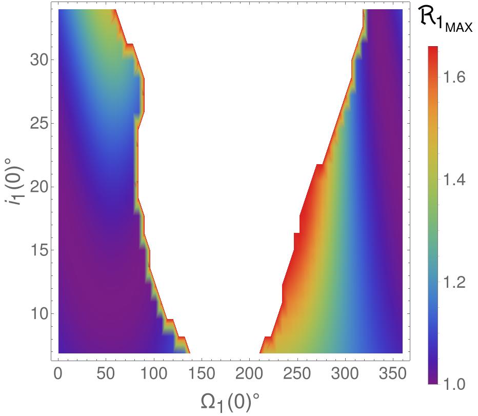
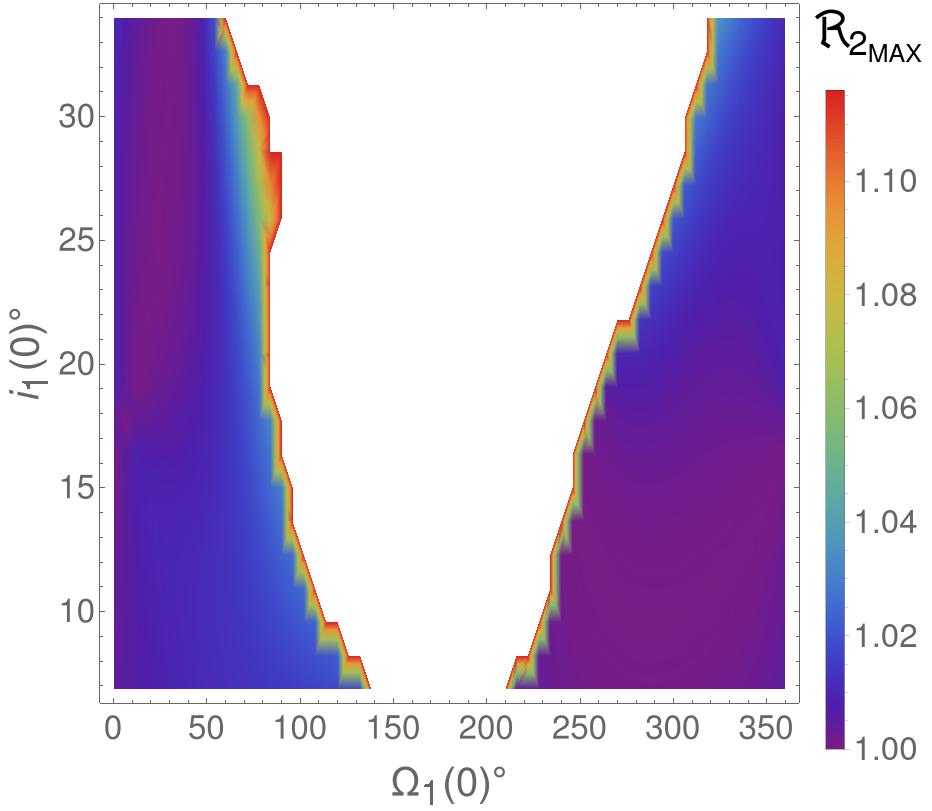
Figure 8: Color-grid plots of the maximal values reached by the ratio $\mathfrak{R}_{1}$ (on the left) and $\mathfrak{R}_{2}\,$ (on the right); see the text for more details.

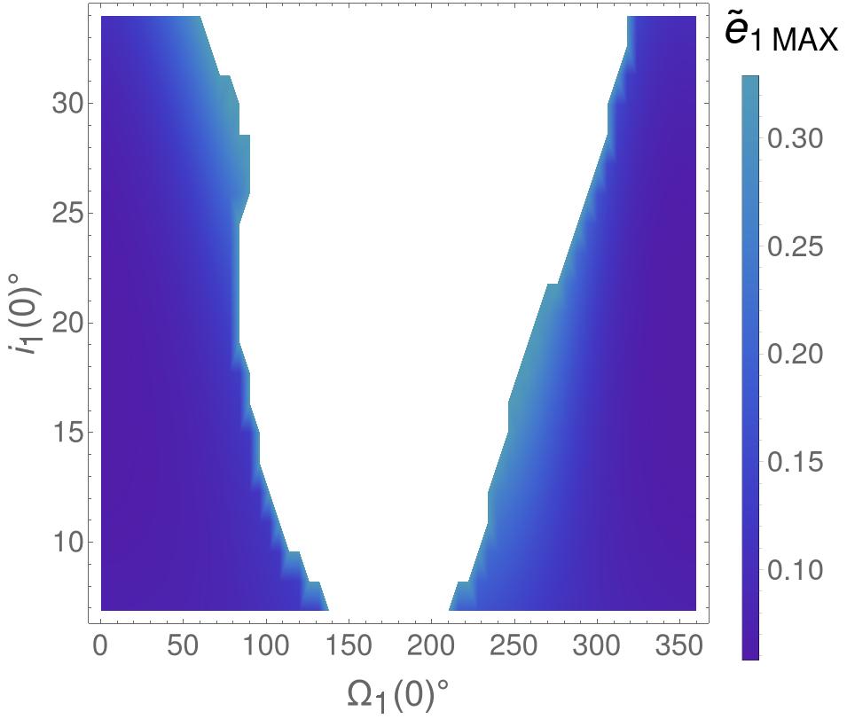
Figure 9: Color-grid plots of the maximum of the function $\tilde{\mathrm{e}}(t)$, which is defined in (64).

Comparing the regions of the stability domain at the border near the (white) central ones, we see that all three numerical indicators plotted in Figures 8–9 increase their values when the unstable zone is approached. This is in agreement with the expectations and the comparison with Figure 2a. On the other hand, the $2$ DOF secular model is unable to capture the region of instability internal to the stable one, highlighted by two green stripes starting from the bottom of Figure 2a in correspondence with $\Omega_{1}(0)=0^{\circ}=360^{\circ}$. The two curved stripes look rather symmetric and they join each other around the point $\big{(}\mathrm{i}_{1}(0)\,,\,\Omega_{1}(0)\big{)}\simeq\big{(}30^{\circ},\,0^{\circ}\big{)}=\big{(}30^{\circ},\,360^{\circ}\big{)}$. Since the dependence of the Hamiltonian on the angles ${\bm{q}}$ (which describes the dynamics of the outer exoplanets) is removed from the $2$DOF model, it seems reasonable that some of the resonances are not present in the normal form generated by the algorithm à la Birkhoff, although they play a remarkable role in the dynamics of more complex models.

6 Secular orbital evolution of $\upsilon$-And $\mathbf{b}$ taking also into account relativistic effects

In this Section we study the dynamics of $\upsilon$-And $\mathbf{b}$ in the framework of a secular quasi-periodic restricted Hamiltonian model where also corrections due to general relativity are taken into account. Since we focus on the orbital dynamics of the innermost planet of the $\upsilon$-Andromedæ system and it is very close to a star that is about 30% more massive than the Sun (let us recall that the value of the semi-major axis of $\upsilon$-And $\mathbf{b}$ is reported in Table 7, i.e., $a_{1}=0.0594$ AU), it is natural to expect that the corrections due to general relativity can play a relevant role for the system under consideration. Similarly as in the previous Sections, we study these effects in the framework of a $2$ DOF secular model. We start by considering the following Hamiltonian:

$$\mathcal{H}=\mathcal{H}_{4BP}+\mathcal{H}_{GR}\,,$$

where $\mathcal{H}_{4BP}$ defines the four body problem (see (9)) and $\mathcal{H}_{GR}$ describes the general (post-Newtonian) relativistic corrections to the Newtonian mechanics. Following [23], the secular quasi-periodic restricted Hamiltonian which includes corrections due to the General Relativity (hereafter, GR) is obtained by removing the dependence of the Hamiltonian on the fast angles. Therefore, we introduce

$$\mathcal{H}^{(GR)}_{sec}=\int_{\mathbb{T}^{3}}\frac{\mathcal{H}_{4BP}}{8\pi^{3}}\,d\lambda_{1}d\lambda_{2}d\lambda_{3}+\int_{\mathbb{T}}\frac{\mathcal{H}_{GR}}{2\pi}\,dM_{1}\,:=\mathcal{H}^{(NG)}_{sec}+\left\langle\mathcal{H}_{{GR}}\right\rangle_{M_{1}}\,,$$ (65)

where the expansion of the mean of the $4BP$ Hamiltonian $\mathcal{H}^{(NG)}_{sec}$ (recall definition (10)) is explicitely written in equation (11), while the average of the GR contribution with respect to the mean anomaly of $\upsilon$-And $\mathbf{b}$ is given by

$$\left\langle\mathcal{H}_{{GR}}\right\rangle_{M_{1}}=-\frac{3\,\mathcal{G}^{2}\,m_{0}^{2}\,m_{1}}{a_{1}^{2}c^{2}\sqrt{1-\mathrm{e}_{1}^{2}}}+\frac{15\,\mathcal{G}^{2}\,m_{0}^{2}\,m_{1}}{8a_{1}^{2}c^{2}}-\frac{\mathcal{G}^{2}\,m_{0}\,m_{1}^{2}}{8a_{1}^{2}c^{2}}\,,$$ (66)

$c$ being the velocity of light in vacuum. In the above expression of $\left\langle\mathcal{H}_{{GR}}\right\rangle_{M_{1}}\,$, the summand where the eccentricity of $\upsilon$-And $\mathbf{b}$ (i.e., $\mathrm{e}_{1}$) occurs in the denominator is the only to be untrivial, in the sense that the other two give additional constant contribution to the secular Hamiltonian and, then, they can be disregarded. By proceeding in a similar way to what has been already done for the classical expansions of the initial Hamiltonian (1), it is possible to express $\left\langle\mathcal{H}_{{GR}}\right\rangle_{M_{1}}$ in the Poincaré variables $(\xi_{1},\eta_{1})$, described in equation (2).

Thus, keeping in mind the procedure explained in Section 3, one easily realizes that the secular quasi-periodic restricted model of the dynamics of $\upsilon$-And $\mathbf{b}$ which includes relativistic corrections (hereafter, SQPR-GR) can be described by the following $2+3/2$ DOF Hamiltonian:

$$\mathcal{H}^{(GR)}_{sec,\,2+\frac{3}{2}}({\bm{p}},{\bm{q}},\xi_{1},\eta_{1},P_{1},Q_{1}) =\omega_{3}\,p_{3}+\omega_{4}\,p_{4}+\omega_{5}\,p_{5}$$ (67)

$$\phantom{=}+\mathcal{H}^{(NG)}_{sec}(q_{3},q_{4},q_{5},\xi_{1},\eta_{1},P_{1},Q_{1})+\left\langle\mathcal{H}_{GR}\right\rangle_{M_{1}}(\xi_{1},\eta_{1})\,,$$

where the angular velocity vector ${\bm{\omega}}=(\omega_{3},\omega_{4},\omega_{5}\,)$ is given in (LABEL:freq.fond.CD) and $\mathcal{H}^{(NG)}_{sec}$ can be replaced by $\mathcal{H}^{1-2}_{sec}+\mathcal{H}^{1-3}_{sec}$ appearing in formula (13). Finally, in the framework of this SQPR-GR model, the equations for the orbital motion of the innermost planet can be written as

$$\begin{cases}\dot{q_{3}}=\partial\mathcal{H}^{(GR)}_{sec,2+\frac{3}{2}}/\partial p_{3}=\omega_{3}\\ \dot{q_{4}}=\partial\mathcal{H}^{(GR)}_{sec,2+\frac{3}{2}}/\partial p_{4}=\omega_{4}\\ \dot{q_{5}}=\partial\mathcal{H}^{(GR)}_{sec,2+\frac{3}{2}}/\partial p_{5}=\omega_{5}\\ \dot{\xi}_{1}=-\partial\left(\mathcal{H}_{sec}^{(NG)}(q_{3},q_{4},q_{5},\xi_{1},\eta_{1},P_{1},Q_{1})+\left\langle\mathcal{H}_{GR}\right\rangle_{M_{1}}(\xi_{1},\eta_{1})\right)/\partial\eta_{1}\\ \dot{\eta}_{1}=\partial\left(\mathcal{H}_{sec}^{(NG)}(q_{3},q_{4},q_{5},\xi_{1},\eta_{1},P_{1},Q_{1})+\left\langle\mathcal{H}_{GR}\right\rangle_{M_{1}}(\xi_{1},\eta_{1})\right)/\partial\xi_{1}\\ \dot{P}_{1}=-\partial\mathcal{H}_{sec}^{(NG)}(q_{3},q_{4},q_{5},\xi_{1},\eta_{1},P_{1},Q_{1})/\partial Q_{1}\\ \dot{Q}_{1}=\partial\mathcal{H}_{sec}^{(NG)}(q_{3},q_{4},q_{5},\xi_{1},\eta_{1},P_{1},Q_{1})/\partial P_{1}\end{cases}\,.$$ (68)

6.1 Numerical integration of the SQPR-GR model

Similarly as in Subsection 3.1.2, we numerically integrate the equations of motion for the secular quasi-periodic restricted Hamiltonian with general relativistic corrections, defined in formula (68). As initial values of the orbital parameters $a_{1}(0)$, $\mathrm{e}_{1}(0)$, $M_{1}(0)$ and $\omega_{1}(0)$ we take those reported in Table 7; moreover, we set $m_{1}=0.674$ as value for the mass of $\upsilon$-And $\mathbf{b}$ and $(\mathrm{i}_{1}(0)\,,\Omega_{1}(0))$ ranging in the $20\times 60$ regular grid that covers $I_{\mathrm{i}}\times I_{\Omega}=[6.865^{\circ},34^{\circ}]\times[0^{\circ},360^{\circ}]$. Hence, it is possible to compute the corresponding initial values of the orbital elements in the Laplace reference frame (which is determined taking into account $\upsilon$-And $\mathbf{c}$ and $\upsilon$-And $\mathbf{d}$ only) and to perform $21\times 60$ numerical integrations starting from all these initial data. Once again, for each numerical integration, we are interested in determining the maximal values reached by the eccentricity of $\upsilon$-And $\mathbf{b}$ and by the maximal mutual inclination between $\upsilon$-And $\mathbf{b}$ and $\upsilon$-And $\mathbf{c}\,$. The results are reported in the color-grid plots of Figure 10.

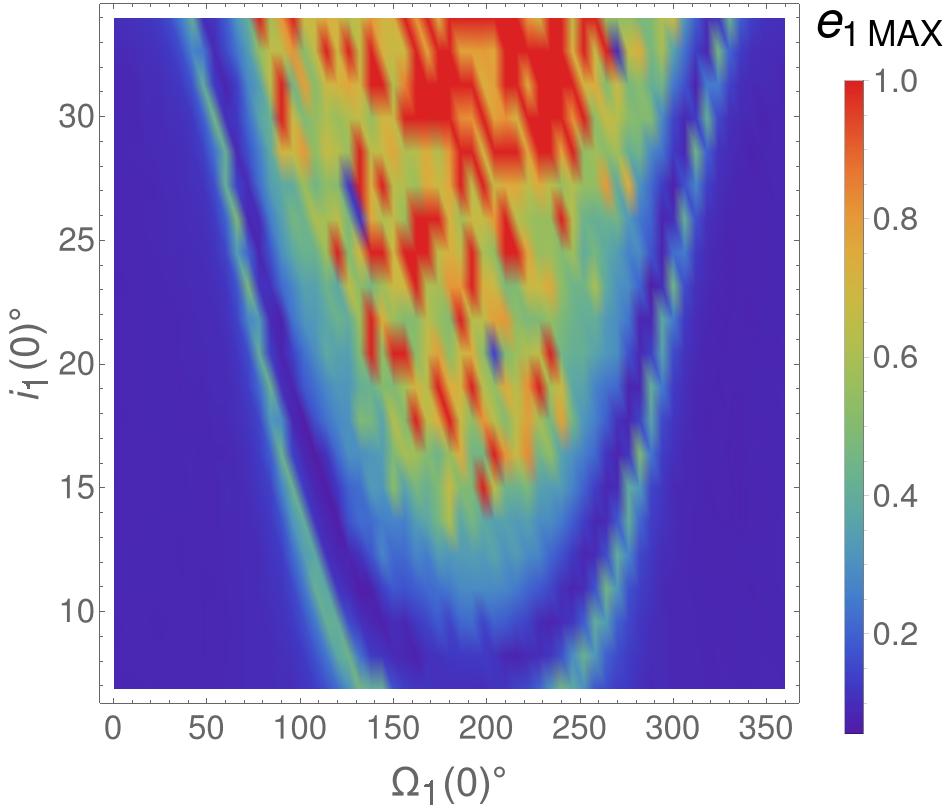
(a)

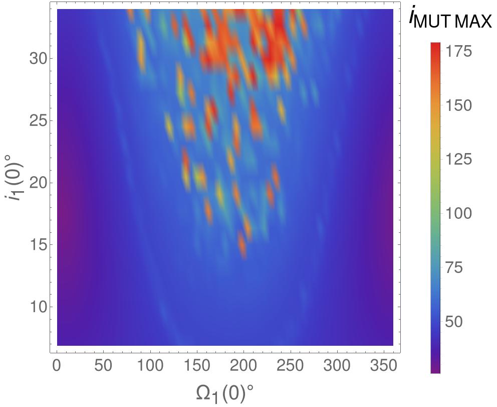
(b)

Figure 10: Color-grid plots of the maximal value reached by the eccentricity of $\upsilon$-And $\mathbf{b}$ (on the left) and by the mutual inclination between $\upsilon$-And $\mathbf{b}$ and $\upsilon$-And $\mathbf{c}$ (on the right). The maxima are computed during the RK4 numerical integrations (each of them covering a timespan of $10^{5}$ yr) of the SQPR-GR equations of motion (68), which cover a timespan of $10^{5}$ yr.

By comparing Figure 10a with Figure 5a, one can immediately realize that the regions colored in blue are much wider in the former than in the latter one. Indeed, the darker regions refer to initial conditions which generate motions with maximal values of the eccentricity of $\upsilon$-And $\mathbf{b}$ that are relatively low, while the zones colored in red or yellow correspond to such large values of the eccentricity implying that those orbits have to be considered unstable. Therefore, our numerical explorations highlight that the effects due to general relativity play a stabilizing role on the orbital dynamics of the innermost planet. This conclusion is in agreement with was already remarked about the past evolution of our Solar System, in particular for what concerns the orbital eccentricity of Mercury (see [15]).

Moreover, as already done in Section 3.1.2, in order to further explore the stable and chaotic regions of Figure 10a, we apply the Frequency Map Analysis method to the signal $\xi_{1}(t)+i\eta_{1}(t)$ as produced by the numerical integration of the system (68), i.e., in the SQPR-GR approximation. We perform the numerical integrations as described at the beginning of the present Section, taking into account only a few values in $I_{\mathrm{i}}\,$ for the initial inclinations, i.e. $\mathrm{i}_{1}(0)=6.865^{\circ},\,8.22175^{\circ},\,9.5785^{\circ},\,10.9353^{\circ}$ and $\Omega_{1}(0)\in I_{\Omega}\,$. In Figure 11 we report the behaviour of the angular velocity $\nu$ corresponding to the first component of the approximation of $\xi_{1}(t)+i\eta_{1}(t)$, as obtained by applying the FA computational algorithm; we recall that this quantity is related to the precession rate of $\varpi_{1}\,$. As initial value for the inclination $\mathrm{i}_{1}(0)$ we fix $6.865^{\circ}$ for Figure 11a and $10.9353^{\circ}$ for Figure 11b. Also here, we do not report the cases $(\mathrm{i}_{1}(0),\Omega_{1}(0))\in\{8.22175^{\circ},\,9.5785^{\circ}\}\times I_{\Omega}\,$, since the behaviour of these plots is similar to the ones in Figure 11.

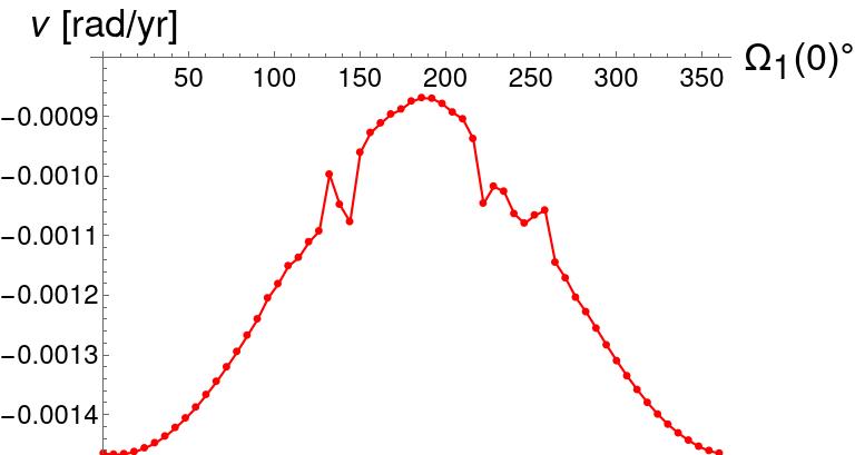
(a)

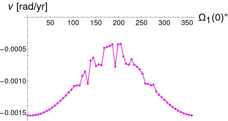
(b)

Figure 11: Behaviour of the fundamental angular velocity $\nu$ as obtained by applying the Frequency Map Analysis method to the signal $\xi_{1}(t)+i\eta_{1}(t)\,$, computed through the RK4 numerical integration of the SQPR-GR model (68), covering a timespan of $1.31072\cdot 10^{5}$ yr. We take, as initial conditions, $(\mathrm{i}_{1}(0),\Omega_{1}(0))\in\{6.865^{\circ}\}\times I_{\Omega}$ for the left panel and $(\mathrm{i}_{1}(0),\Omega_{1}(0))\in\{10.9353^{\circ}\}\times I_{\Omega}$ for the right one.

The situation is well described by Figure 11a and analogous considerations hold for Figure 11b apart a few main differences which will be highlighted in the following discussion. When the values of $\Omega_{1}(0)$ are ranging in $[0,\sim 120^{\circ}]$ and $[\sim 260^{\circ},\,360^{\circ}]$ we can observe a regular behaviour of the angular velocity $\nu$ which is also nearly monotone, with the only exception around a local minimum. According to the Frequency Map Analysis method, such a regular regime is due to the presence of many invariant tori which fill the stability region located at the two lateral sides of the plot 10a. In the case of Figure 11a, this also applies when $\Omega_{1}(0)$ is ranging in $[\sim 150^{\circ},\sim 220^{\circ}]$, which corresponds to the stable blue internal area of Figure 10a. On the other hand, in the case of Figure 11b, for the same range of initial values of the node longitude of $\upsilon$-And $\mathbf{b}$, the behaviour is not so regular; this is in agreement with the fact that in correspondence with $\mathrm{i}_{1}(0)\sim 11^{\circ}$ the plot of the maximal values of $\mathrm{e}_{1}$ in the central region highlights the occurrence of chaotical phenomena. Moreover, for what concerns values of $\Omega_{1}(0)$ in $[\sim 120^{\circ},\,\sim 150^{\circ}]$ and $[\sim 220^{\circ},\,\sim 260^{\circ}]$ (corresponding to the green stripes of Figure 10a), Figure 11a shows a behaviour typical of the crossing of a resonance in the chaotic region surrounding a separatrix. The value of the angular velocity for which this phenomenon takes place is, again, related to $\omega_{4}\simeq-1.04\cdot 10^{-3}$ (as it can be easily appreciated looking to the small plateau appearing in Figure 11b).

Comparing Figure 11 with Figure 6 the enlargement of the stable region is evident. Moreover, we can also see how much this phenomenon is influenced by the modification of the pericenter precession rate of the inner planet due to relativistic effects. Indeed, looking at the values reported on the $y$-axis of Figures 11 and 6, one can appreciate that the fundamental angular velocity, in the case of the SQPR model, takes values remarkably closer to zero with respect to those assumed in the case of the SQPR-GR model.

6.2 Application of the normalization algorithms to the secular quasi-periodic restricted model of the dynamics of $\upsilon$-And $\mathbf{b}$ with relativistic corrections

Starting from Hamiltonian (67), we can reapply the normalization algorithms described in Subsections 4.1 and 4.2. All this computational procedure ends up with the introduction of a new $2$ DOF Hamiltonian model which can be written in the following form (analogous to the one reported in formula (53)):

$$\begin{aligned} \mathcal{H}_{2DOF}^{(GR)}({\bm{I}},{\bm{\alpha}})&=\mathcal{E}_{B;GR}+{\bm{\Omega}}_{B;GR}\cdot{\bm{I}}+\sum_{s=0}^{\mathcal{N}_{S}}\sum_{l=3}^{\mathcal{N}_{L}}h_{l}^{(\mathcal{N}_{L}-2,s)}({\bm{I}},{\bm{\alpha}})\,,\end{aligned}$$ (69)

where $\mathcal{E}_{B;GR}\in\mathbb{R}$, ${\bm{\Omega}}_{B;GR}\in\mathbb{R}^{2}$ and $h_{l}^{(\mathcal{N}_{L}-2,s)}\in\mathfrak{P}_{l,2s}$ $\forall\ l=3,\,\ldots\,,\,\mathcal{N}_{L}\,,\>s=0\,,\,\ldots\,,\,\mathcal{N}_{S}\,$. We emphasize that also $\mathcal{H}_{2DOF}^{(GR)}$ is integrable because of the same reasons already discussed in Section 5; indeed, after having checked that ${\partial\mathcal{H}_{2DOF}^{(GR)}}/{\partial\alpha_{1}}\,+\,{\partial\mathcal{H}_{2DOF}^{(GR)}}/{\partial\alpha_{2}}\,=\,0\,$, we can apply the Liouville theorem, because there are two independent constants of motion, i.e., $I_{1}+I_{2}$ and $\mathcal{H}_{2DOF}^{(GR)}$ itself.

Moreover, also for this new model we can reproduce the same kind of numerical exploration described in Section 5. In particular, we can compute the values of the numerical indicators $\mathfrak{R}_{1\,{\rm MAX}}\,$, $\mathfrak{R}_{2\,{\rm MAX}}$ and $\tilde{\mathrm{e}}_{1\,{\rm MAX}}$ corresponding to each pair $\big{(}\mathrm{i}_{1}(0),\Omega_{1}(0)\big{)}\,$ of the $21\times 60$ points definining the regular grid which covers $I_{\mathrm{i}}\times I_{\Omega}=[6.865^{\circ},34^{\circ}]\times[0^{\circ},360^{\circ}]$. In the following, we analyze the color-grid plots for a few different values of the parameter ruling the truncation in the trigonometric degree, namely $\mathcal{N}_{S}\,$, and in the square root of the action, i.e., $\mathcal{N}_{L}\,$. The color-grid plots for the maximal value reached by $\mathfrak{R}_{1}\,$ and $\tilde{\mathrm{e}}_{1}$ are reported in Figures 12–14.

Let us recall that $\mathfrak{R}_{2\,{\rm MAX}}$ is an evaluation of the maximal excursion of the inclination of $\upsilon$-And $\mathbf{b}$. For the sake of brevity, its plots are omitted and they are not included in Figures 12–14, because in our numerical explorations the ranges of values experienced by $\mathfrak{R}_{2\,{\rm MAX}}$ are so narrow that their analysis does not look so significant. Therefore, it is better to focus on the plots of $\mathfrak{R}_{1\,{\rm MAX}}$ and $\tilde{\mathrm{e}}_{1\,{\rm MAX}}\,$; let us recall that both of them refer to the eccentricity of $\upsilon$-And $\mathbf{b}$. By comparing Figures 12–14, one can appreciate a well known phenomenon concerning the constructive algorithms à la Birkhoff: the greater the number of normalization steps (i.e., $\mathcal{N}_{L}-2$), the smaller the domain of applicability (see, e.g., [6] for the discussion about the determination of the optimal step).

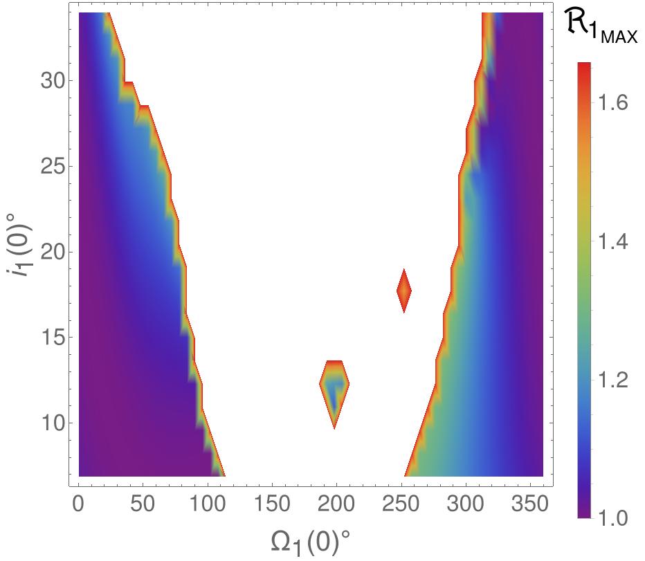
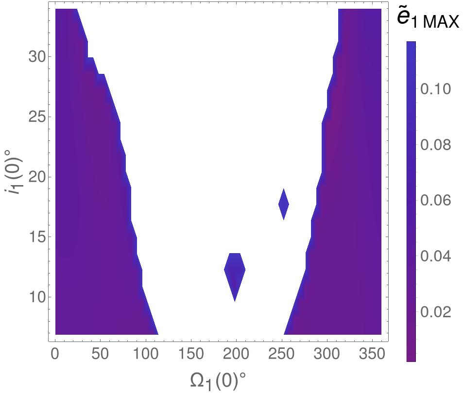
Figure 12: Color-grid plots of the maximal values reached by the ratio $\mathfrak{R}_{1}(t)$ (on the left) and the function $\tilde{\mathrm{e}}(t)$ (on the right), which are defined in (63)–(64). These laws of motion are computed along the flow induced by the $2$ DOF Hamiltonian $\mathcal{H}_{2DOF}^{(GR)}$ which takes into account also GR corrections and is defined in (69), in the particular case with $\mathcal{N}_{S}=5$ and $\mathcal{N}_{L}=6$.

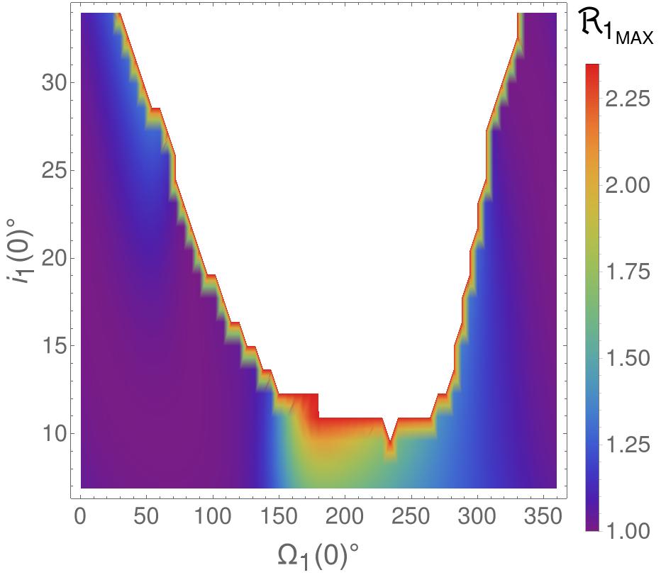
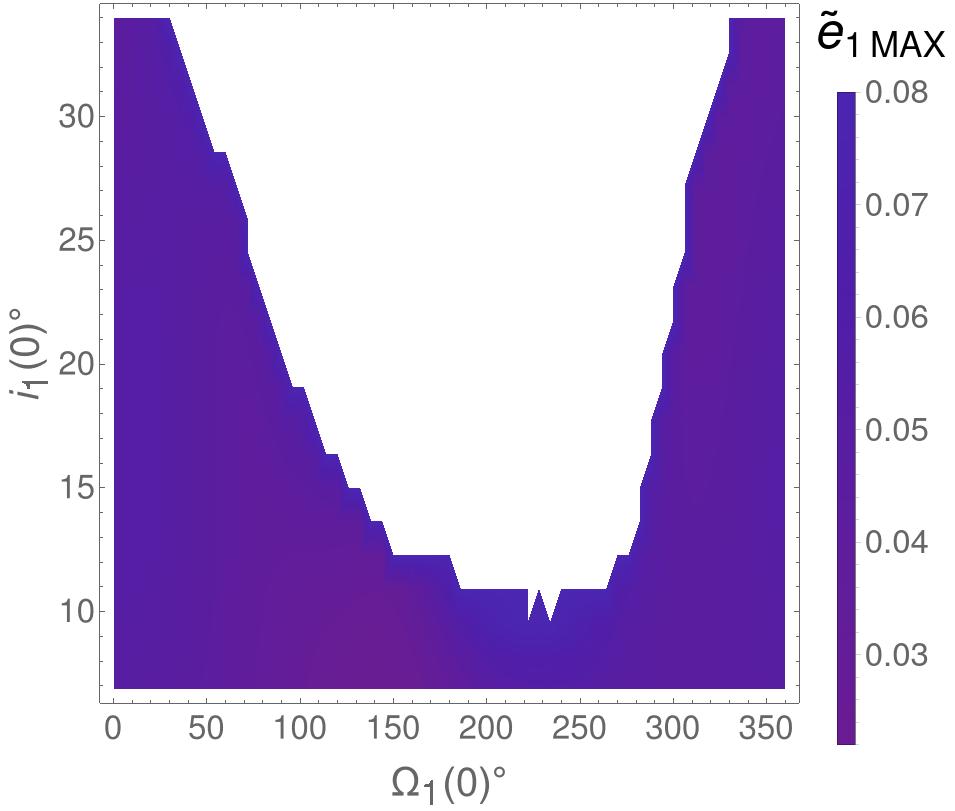
Figure 13: Same as in Figure 12, in the case with $\mathcal{N}_{S}=6$ and $\mathcal{N}_{L}=5$.

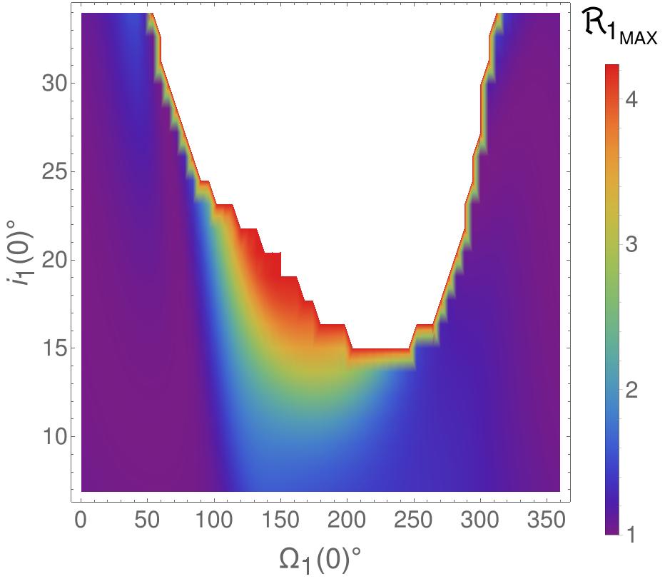
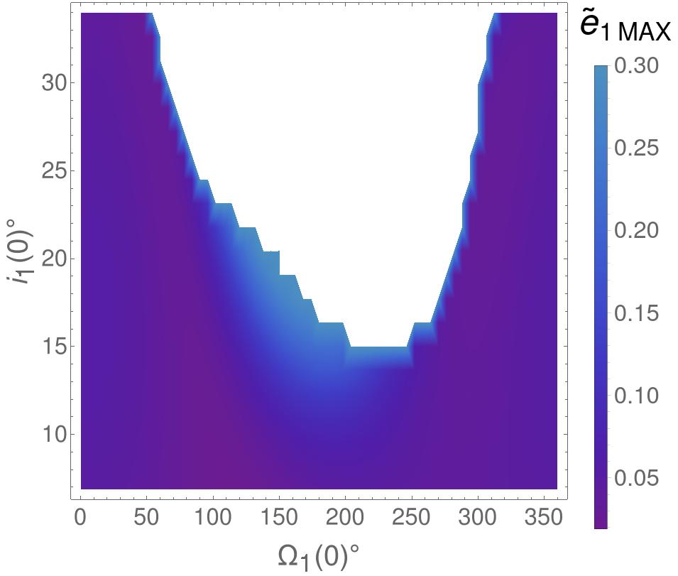
Figure 14: Same as in Figure 12, in the case with $\mathcal{N}_{S}=6$ and $\mathcal{N}_{L}=4$.

By comparing Figures 13–14 also with Figure 10a, we observe that in the cases with $\mathcal{N}_{L}=4,\,5$ our computational procedure is able to reconstruct with a good accuracy the $U$–shaped border of the stability domain. Note that the horizontal strip at the bottom of the plots corresponds to orbital motions which look stable, since the eccentricity of $\upsilon$-And $\mathbf{b}$ does not reach large values (with the eventual exception of the narrow green areas that in Figure 10a are expected to correspond to resonant regions). This highlights a main difference with the non-relativistic model discussed in Section 5, because in that case there is an interval of values of $\Omega_{1}(0)$ centered about $180^{\circ}$ for which none of the initial inclinations $\mathrm{i}_{1}(0)\in[6.865^{\circ},34^{\circ}]$ corresponds to a stable orbital configuration (see Figure 5a). The reliability of our simplified $2$ DOF Hamiltonian model (which is defined in formula (69) and takes into account also GR corrections) is enforced also by the fact that it is able to capture also this phenomenon.

References

- [1] R. P. Butler, G. W. Marcy, D. A. Fischer, T. M. Brown, A. R. Contos, S. G. Korzennik, P. Nisenson, and R. W. Noyes. Evidence for multiple companions to Andromedae. The Astrophysical Journal, 526(2):916, dec 1999.
- [2] C. Caracciolo. Normal form for lower dimensional elliptic tori in Hamiltonian systems. Mathematics in Engineering, 4(6):1–40, 2022.
- [3] C. Caracciolo, U. Locatelli, M. Sansottera, and M. Volpi. Librational KAM tori in the secular dynamics of the Andromedæ planetary system. Monthly Notices of the Royal Astronomical Society, 510(2):2147–2166, 2022.
- [4] S. Curiel, J. Cantó, L. Georgiev, C. Chávez, and A. Poveda. A fourth planet orbiting Andromedae. Astronomy & Astrophysics, 525:A78, 2011.
- [5] R. Deitrick, R. Barnes, B. McArthur, T. R. Quinn, R. Luger, A. Antonsen, and G. F. Benedict. The three-dimensional architecture of the andromedae planetary system. The Astrophysical Journal, 798(1):46, 2015.
- [6] A. Giorgilli. Notes on exponential stability of Hamiltonian systems. Pubblicazioni della Classe di Scienze, Scuola Normale Superiore, Pisa. Centro di Ricerca Matematica “Ennio De Giorgi”, 2003.
- [7] A. Giorgilli. Notes on Hamiltonian Dynamical Systems, volume 102. Cambridge University Press, 2022.
- [8] A. Giorgilli, A. Delshams, E. Fontich, L. Galgani, and C. Simó. Effective stability for a Hamiltonian system near an elliptic equilibrium point, with an application to the restricted three–body problem. J. Differential Equations, 77:167–198, 1989.
- [9] A. Giorgilli, U. Locatelli, and M. Sansottera. On the convergence of an algorithm constructing the normal form for lower dimensional elliptic tori in planetary systems. Celestial Mechanics and Dynamical Astronomy, 119:397–424, 2014.
- [10] A. Giorgilli, U. Locatelli, and M. Sansottera. Secular dynamics of a planar model of the Sun-Jupiter-Saturn-Uranus system; effective stability in the light of Kolmogorov and Nekhoroshev theories. Regular and Chaotic Dynamics, 22:54–77, 2017.
- [11] W. Gröbner. Die Lie-reihen und ihre Anwendungen, volume 3. Deutscher Verlag der Wissenschaften, 1967.
- [12] N. H. Hoang, F. Mogavero, and J. Laskar. Long-term instability of the inner Solar System: numerical experiments. Monthly Notices of the Royal Astronomical Society, 514(1):1342–1350, 2022.
- [13] J. Laskar. Introduction to Frequency Map Analysis. In C. Simó, editor, Hamiltonian Systems with Three or More Degrees of Freedom, pages 134–150. Springer Netherlands, Dordrecht, 1999.
- [14] J. Laskar. Frequency map analysis and quasiperiodic decompositions. In E. Lega, D. Benest, and C. Froeschlé, editors, Hamiltonian systems and Fourier analysis: new prospects for gravitational dynamics. Cambridge Scientific Pub Ltd, 2005.
- [15] J. Laskar and M. Gastineau. Existence of collisional trajectories of Mercury, Mars and Venus with the Earth. Nature, 459(7248):817–819, 2009.
- [16] J. Laskar and P. Robutel. High order symplectic integrators for perturbed Hamiltonian systems. Celestial Mechanics and Dynamical Astronomy, 80(1):39–62, 2001.
- [17] U. Locatelli, C. Caracciolo, M. Sansottera, and M. Volpi. Invariant KAM tori: from theory to applications to exoplanetary systems. I-Celmech training school, Springer PROMS, 2022.
- [18] U. Locatelli, C. Caracciolo, M. Sansottera, and M. Volpi. A numerical criterion evaluating the robustness of planetary architectures; applications to the Andromedæ system. Proceedings of the International Astronomical Union, 15(S364):65–84, 2022.
- [19] U. Locatelli and A. Giorgilli. Invariant tori in the secular motions of the three-body planetary systems. Celestial Mechanics and Dynamical Astronomy, 78(1):47–74, 2000.
- [20] R. Mastroianni. Hamiltonian secular theory and KAM stability in exoplanetary systems with 3D orbital architecture. PhD Thesis, Dep. of Mathematics “Tullio-Levi Civita”, Univ. of Padua, 2023.
- [21] M. Mayor and D. Queloz. A Jupiter-mass companion to a solar-type star. Nature, 378(6555):355–359, 1995.
- [22] B. E. McArthur, G. F. Benedict, R. Barnes, E. Martioli, S. Korzennik, E. Nelan, and R. P. Butler. New observational constraints on the Andromedae system with data from the Hubble Space Telescope and Hobby-Eberly Telescope. The Astrophysical Journal, 715(2):1203–1220, 2010.
- [23] C. Migaszewski and K. Goździewski. Secular dynamics of a coplanar, non-resonant planetary system under the general relativity and quadrupole moment perturbations. Monthly Notices of the Royal Astronomical Society, 392(1):2–18, 2009.
- [24] F. Mogavero and J. Laskar. The origin of chaos in the Solar System through computer algebra. Astronomy & Astrophysics, 662:L3, 2022.
- [25] A. Morbidelli. Modern celestial mechanics: aspects of solar system dynamics. 2002.
- [26] C. D. Murray and S. F. Dermott. Solar system dynamics. Cambridge university press, 1999.
- [27] D. Piskorz, B. Benneke, N. R. Crockett, A. C. Lockwood, G. A. Blake, T. S. Barman, C. F. Bender, J. S. Carr, and J. A. Johnson. Detection of water vapor in the thermal spectrum of the non-transiting hot Jupiter Upsilon Andromedae b. The Astronomical Journal, 154(2):78, 2017.
- [28] M. Volpi, A. Roisin, and A.-S. Libert. The 3D secular dynamics of radial-velocity-detected planetary systems. Astronomy & Astrophysics, 626:A74, 2019.