Curvature Estimates of Nodal Sets of Harmonic Functions in the Plane

Abstract.

In this paper we study curvature estimates for nodal sets of harmonic functions in the plane. We prove that at any point $p$, the curvature of any nodal curve of a harmonic function $u$ is upper bounded by

$$\left|\kappa(u)(p)\right|\leq\frac{8}{nr},$$

where $u$ has only $n$ nodal curves in $B_{r}(p)$ across $p$. This result is sharp, for which the equality case can be characterized when $u$ is the real part of some holomorphic function related to Koebe functions. This curvature estimate was known only for $n=1$ by Ü. Kuran. Our result extends it to general case, and yields the equality case. Thus we prove that, for harmonic functions, the curvature of every nodal curve at any point $p$ is upper bounded by the distance between $p$ and other nodal curves, and the distance from $p$ to the boundary of the domain.

1. Introduction

The study of nodal sets of harmonic functions is an active research area in the geometric theory of PDEs dating back to the origins of potential theory. Analytically, the length of nodal curves of solutions of elliptic equations in the plane is bounded by the area of the region and the gradient of the solution [AG]. For hamonic functions on $\mathbb{R}^{n}$ ($n\geq 2$), Hausdorff measures of nodal sets and singular sets are bounded by the frequency of harmonic functions [HL]. Geometrically, in $\mathbb{R}^{2}$, the nodal set of any harmonic function $u$ at some point $p$ can be locally biholomorphic to $\{z\in\mathbb{C}|Re\,z^{n}=0\}$, where $n$ is the vanishing order of $u$ at $p$, and the nodal set constitutes of some maximal analytic curves [WWZ], which are called nodal curves. In particular, the nodal set of a harmonic function at any non-critical point $p$ is a nodal curve. Moreover, Ü. Kuran first proved in 1969 that at any non-critical point $p$, the curvature of the nodal curve of a harmonic function is upper bounded and the bound depends only on the distance from $p$ to the boundary and to other nodal curves, see [K]. De Carli and Hudson gave another proof in [CH]. Stefan Steinerberger discovered the equivalent condition when the equality holds in the estimate [SS]. Some subtle examples of nodal sets of harmonic functions were shown in [F, FDH, EAD]. Besides, topological properties and the shape properties of nodal sets of elliptical PDEs were given in [SP, BM, KW].

For hamonic functions on $\mathbb{R}^{n}$ ($n\geq 2$), a positive lower bound for the principal curvature of strict convex nodal sets has been proved in [CAMY]. More convexity results related to solutions of linear or nonlinear elliptical PDEs can be found in [KB, BBJ, CA, GRM]. There are also some remarkable results about solutions of elliptical PDEs on annuli, see [DNJ, JJMO]. However, the results mentioned above are about non-critical points, while few results related to critical points were proved.

This paper aims to show that in $\mathbb{R}^{2}$, even at any critical point of a harmonic funtion, the curvature of any nodal curve at that point can be bounded, which is the main result of the paper, see Theorem 2. Therefore, at any point of the nodal set, the curvature is always bounded. This geometric property tells us that the nodal set cannot ‘bend very much’, corresponding to the analytic property that the Hausdorff measure of nodal sets is bounded.

We assume that a harmonic funtion $u$ is defined on a connected region $\Omega$, and $u$ is not a constant. The vanishing order of $u$ at a point $p\in\Omega$ is denoted by $n(u,p)$. The nodal set of $u$ is denoted by $\Gamma$. We identify $\mathbb{R}^{2}$ with $\mathbb{C}$, so that in any ball $B_{r}(p)\subset\Omega$, we can find a holomophic function $f$ satisfying

$$f(z)=u(z)+iv(z),$$

where $v(z)$ is the conjugate function of $u$ in $B_{r}(p)$.

The partial derivatives $\partial u/\partial x$ and $\partial u/\partial y$ are abbreviated as $u_{x}$ and $u_{y}$ respectively. Let $\kappa(u)(p)$ be the curvature of some nodal curve of $u$ at the point $p$.

The following theorem was proved by Ludwig Bieberbach [BL] in 1916. This is the main ingredient for our proof of curvature estimates. Here is the statement:

Theorem 1.

(Bieberbach) Let $f:B_{1}(0)\rightarrow\mathbb{C}$ be holomorphic and injective in $B_{1}(0)$. Assume $f$ has Taylor series of the form

$$f(z)=z+\sum_{n\geq 2}a_{n}z^{n},$$

i.e. $f(0)=0,f^{\prime}(0)=1$. Then the following inequality holds,

$$\left|a_{2}\right|\leq 2.$$

Moreover, the equality holds if and only if

$$f(z)=k_{\theta}(z)=\frac{z}{\left(1-e^{i\theta}z\right)^{2}},$$

where $e^{i\theta}=a_{2}/2$, and $k_{\theta}(z)$ is called rotated Koebe function.

With Bieberbach Theorem, we can prove our main theorem.

Theorem 2.

Let $\Omega$ be a region, $u:\Omega\subseteq\mathbb{R}^{2}\rightarrow\mathbb{R}$ be a non-constant harmonic function satisfying $u(p)=0$, and $r$ be the maximal distance satisfying $u$ has only $n$ nodal curves intersecting at $p$ in $B_{r}(p)\subset\Omega$. Then

$$\left|\kappa(u)(p)\right|\leq\frac{8}{nr}.$$

Moreover, the equality holds if and only if $u(z)=A\cdot\Re f(\frac{z-p}{r}e^{i\alpha})$, where $A$ and $\alpha$ is a constant and

$$f(z)=\frac{z^{n}(1+e^{i\tilde{\theta}_{k}}z)}{(1-e^{i\tilde{\theta}_{k}}z)^{3}},$$

where $\tilde{\theta}_{k}=-\frac{(n+1)}{n}(k\pi+\frac{1}{2}\pi)$ and $k\leq n-1$ is a non-negative integer.

The case $n=1$ is the result proved by Ü. Kuran [K], using Poisson integrals. In fact, Ü. Kuran proved the same result in higher dimensions as well. And the equality case of $n=1$ was proved by Stefan Steinerberger [SS]. But for general cases when $n\geq 2$, it is difficult to derive curvature estimates by Poisson integrals.

In this paper, our proof of the main theorem relies on the complex analysis, regarding any harmonic function $u$ as the real part of some holomorphic function $f$. As nodal curves in nodal set are all analytic, the curvature of each curve exists even at critical points of $u$. Furthermore, by expending the curvature calculation formula along a fixed nodal curve, we prove that the curvature at $p$ depends only on the ratio of $f^{(n+1)}(0)$ and $f^{(n)}(0)$. With Cauchy’s argument principle and a subtle observation, we can prove the number of zeros of $f$ is just $n$, which tells us $f(z)=z^{n}h(z)$, where $h(z)$ is a holomorphic function in $B_{1}(0)$ and never vanishes. Applying Bieberbach Theorem to the primitive function of $h(z)$, we can derive the ratio of $f^{(n+1)}(0)$ and $f^{(n)}(0)$, which gives the inequality. The equality case is also from the equality case in Bieberbach Theorem.

Besides the main theorem, we can also derive another curvature estimate by Bieberbach Theorem, with a somehow stronger condition.

Theorem 3.

Let $\Omega$ be a region, $u:\Omega\subseteq\mathbb{R}^{2}\rightarrow\mathbb{R}$ be a non-constant harmonic function with vanishing order $n=n(u,p)\geq 1$, and let $d$ be the maximal distance that satisfies $\nabla^{n}u$ never vanishes in $B_{d}(p)\subset\Omega$. Then

$$\left|\kappa(u)(p)\right|\leq\frac{8}{n(n+1)d}.$$

In particular, the equality holds if and only if $u(z)=A\cdot\Re f(\frac{z-p}{d}e^{i\alpha})$ in the ball $B_{d}(p)\subset\Omega$, where $A$ and $\alpha$ is a constant and f is represented by

$$f(z)=\sum_{m=1}^{+\infty}\frac{m!}{(m+n-1)!}e^{i(m-1)\tilde{\theta}_{k}}z^{m+n-1},$$

where $\tilde{\theta}_{k}=-\frac{(n+1)}{n}(k\pi+\frac{1}{2}\pi)$ and $k\leq n-1$ is a non-negative integer.

2. curvature estimates of intersecting nodal curves

We first note that locally, $u$ is the real part of some analytic function $f(z)$. After setting $f(p)=0$, the vanishing order $n(u,p)$ is just the vanishing order of $f$ at $p$ (Recall $f^{\prime}(p)=u_{x}(p)-iu_{y}(p)$). So locally, there exists a complex constant $c$, so that $\Re\ c(z-p)^{n(u,p)}$ can be an asymptotic formula of $u(z)$ at $p$. Therefore, there are $n(u,p)$ curves intersecting at $p$, whose tangents divide $2\pi$ equally. Moreover, the curves are analytic. See [WWZ] for more details.

By assuming $n(u,p)=1$ in $B_{r}(p)$, we know that there is only one nodal curve across $p=(x_{p},y_{p})$. After a certain rotation, we can have $u_{x}(p)\neq 0$ and take $x$ locally as a smooth function about $y$. By the implicit function theorem, if $u_{x}(x(y),y)\neq 0$, then we obtain a small neighborhood of $p$, in which

$$x^{\prime}(y)=-\frac{u_{y}(x(y),y)}{u_{x}(x(y),y)}.$$

Differentiate the above formula, we get

$$x^{\prime\prime}(y_{p})=\frac{-u_{y}(p)^{2}u_{xx}(p)+2u_{x}(p)u_{y}(p)u_{xy}(p)-u_{x}(p)^{2}u_{yy}(p)}{u_{x}(p)^{3}}.$$

It is well known that the curvature of the graph of a function $x=x(y)\in C^{2}(\mathbb{R})$ at a point $p=(x(y),y)$ can be expressed as follow:

$$\kappa(x)(p)=\frac{x^{\prime\prime}(y)}{\left(1+[x^{\prime}(y)]^{2}\right)^{3/2}}.$$

So, we have

(2.1) $$\quad\kappa(u)(p)=\frac{-u_{y}(p)^{2}u_{xx}(p)+2u_{x}(p)u_{y}(p)u_{xy}(p)-u_{x}(p)^{2}u_{yy}(p)}{\left(u_{x}(p)^{2}+u_{y}(p)^{2}\right)^{3/2}}.$$

In fact, the calculation above does not need $u_{x}(x(y),y)\neq 0$.

Through simple calculation, setting $u=\Re f$, we can easily derive the following formula

(2.2) $$\kappa(u)(p)=\left|f^{\prime}(p)\right|\Re\left(\frac{f^{\prime\prime}(p)}{(f^{\prime}(p))^{2}}\right).$$

See [RPJ] for more details.

First, we have the following essential estimate:

Lemma 4.

Let $u$ be a harmonic function defined in $B_{r}(0)$, with $u(z)=\Re f(z)$, and satisfy $u(0)=0,\forall k\leq n-1,\,\nabla^{k}u(0)=0$ (as a tensor of order $k$), while $\nabla^{n}u(0)\neq 0$ (where $n=n(u,0)\geq 1$ is the vanishing order of u at $0$). Let $\kappa$ be the curvature of some curve $\gamma$ of the nodal set at the origin, then we have:

(2.3) $$\left|\kappa(u)(0)\right|\leq\frac{2}{n^{2}+n}\left|\frac{f^{(n+1)}(0)}{f^{(n)}(0)}\right|.$$

Moreover, the equality holds if and only if

$$f^{(n+1)}(0)=e^{-i(n+1)\theta_{k}}\left|f^{(n+1)}(0)\right|$$

where

$$\theta_{k}=\frac{k\pi+\frac{1}{2}\pi-arg(f^{(n)}(0))}{n},\qquad 0\leq k\leq n-1.$$

Proof.

By $Cauchy-Riemann$ equations, we have: $\partial f/\partial z=\partial f/\partial z+\partial f/\partial\bar{z}=\partial f/\partial x=u_{x}-iu_{y}$, therefore

$$f^{(n)}=\frac{\partial^{n}f}{\partial z^{n}}=\frac{\partial^{n}u}{\partial x^{n}}-i\frac{\partial^{n}u}{\partial x^{n-1}\partial y}.$$

Let $\gamma$ be parametrized by arc length, and $\gamma(0)=0$. Along $\gamma=\gamma(t)$ (i.e. $z=\gamma(t)$), by expension we have

(2.4) $$0=\Re\,f(\gamma(t))=\Re\,\left(\frac{z^{n}}{n!}f^{(n)}(0)+\frac{z^{n+1}}{(n+1)!}f^{(n+1)}(0)+o(z^{n+1})\right),$$

where $o(z^{n+1})$ satisfies $\lim\limits_{z\rightarrow 0}o(z^{n+1})/z^{n+1}=0$. Thus along $\gamma$:

$$\Re\,\left(\frac{z^{n}}{n!}f^{(n)}(0)\right)=-\Re\,\left(\frac{z^{n+1}}{(n+1)!}f^{(n+1)}(0)+o(z^{n+1})\right),\quad z=\gamma(t)\rightarrow 0.$$

Specially, $\gamma$ approaches the origin as

$$\Re\,\frac{\gamma(t)^{n}f^{(n)}(0)}{\left|\gamma(t)\right|^{n}}\rightarrow 0.$$

By setting $\gamma(t)=r(t)e^{i\theta(t)}$, we get an integer $k$ satisfying $0\leq k\leq n-1$ and

$$\theta(t)=\frac{k\pi+\frac{1}{2}\pi-arg(f^{(n)}(0))}{n}+o(1),\qquad 0\leq k\leq n-1.$$

Denoting $\theta_{k}:=\lim\limits_{t\rightarrow 0}\theta(t)$, we have $\theta(t)=\theta_{k}+o(1)$. Thus,

(2.5) $$\Re\,\left(e^{in\theta_{k}}f^{(n)}(0)\right)=0.$$

Without loss of generality, we assume $f^{(n)}(0)=\pm ie^{-in\theta_{k}}\left|f^{(n)}(0)\right|$.

On the other hand, expand $f^{\prime}(z)$ and $f^{\prime\prime}(z)$ at the origin:

$$f^{\prime}(z) = \frac{z^{n-1}}{(n-1)!}f^{(n)}(0)+\frac{z^{n}}{n!}f^{(n+1)}(0)+o(z^{n})$$

$$f^{\prime\prime}(z) = \frac{z^{n-2}}{(n-2)!}f^{(n)}(0)+\frac{z^{n-1}}{(n-1)!}f^{(n+1)}(0)+o(z^{n-1}).$$

Because every nodal curve is analytic [WWZ], the curvature of each nodal curve at the origin exists and is continuous. Thus we only need to take the limit of the curvature to calculate $\kappa(u)(0)$. Combined with equation(2.2) we have ($z=\gamma(t)\rightarrow 0$)

$$\kappa(u)(0)=\lim\limits_{z\rightarrow 0}\left|f^{\prime}(z)\right|\Re\,\left(\frac{f^{\prime\prime}(z)}{(f^{\prime}(z))^{2}}\right)$$

$$= \lim\limits_{z\rightarrow 0}\frac{\Re\,\left(f^{\prime\prime}(z)(\overline{f^{\prime}(z)})^{2}\right)}{\left|f^{\prime}(z)\right|^{3}}$$

$$= \lim\limits_{z\rightarrow 0}\left(\frac{\Re\,\left(\frac{\bar{z}^{n}|z|^{2(n-2)}\overline{f^{(n)}(0)}\left|f^{(n)}(0)\right|^{2}}{(n-2)!(n-1)!(n-1)!}+\frac{2\bar{z}^{n+1}|z|^{2(n-2)}\overline{f^{(n+1)}(0)}\left|f^{(n)}(0)\right|^{2}}{(n-2)!(n-1)!n!}\right)}{\left|\frac{z^{n-1}}{(n-1)!}f^{(n)}(0)\right|^{3}}\right.$$

$$+ \left.\frac{\Re\,\left(\frac{\bar{z}^{n-1}|z|^{2(n-1)}(\overline{f^{(n)}(0)})^{2}f^{(n+1)}(0)}{(n-1)!(n-1)!(n-1)!}\right)}{\left|\frac{z^{n-1}}{(n-1)!}f^{(n)}(0)\right|^{3}}\right)$$

$$\left(\text{combined with equation (\ref{E3.10}), and note}\ \Re\,(\overline{z^{n}f^{(n)}(0)})=\mathrm{Re}\,(z^{n}f^{(n)}(0))\right)$$

$$= \lim\limits_{z\rightarrow 0}\frac{\Re\,\left(\frac{(n+2)\bar{z}^{n+1}|z|^{2(n-2)}\overline{f^{(n+1)}(0)}\left|f^{(n)}(0)\right|^{2}}{(n-2)!(n-1)!(n+1)!}+\frac{\bar{z}^{n-1}|z|^{2(n-1)}(\overline{f^{(n)}(0)})^{2}f^{(n+1)}(0)}{(n-1)!(n-1)!(n-1)!}\right)}{\left|\frac{z^{n-1}}{(n-1)!}f^{(n)}(0)\right|^{3}}.$$

The infinitesimals above are all $o(z^{3(n-1)})$, so we omit them. For the first term in the last equation, we get

$$I = \lim\limits_{z\rightarrow 0}\frac{\Re\,\left(\frac{(n+2)\bar{z}^{n+1}|z|^{2(n-2)}\overline{f^{(n+1)}(0)}\left|f^{(n)}(0)\right|^{2}}{(n-2)!(n-1)!(n+1)!}\right)}{\left|\frac{z^{n-1}}{(n-1)!}f^{(n)}(0)\right|^{3}}$$

$$= \lim\limits_{z\rightarrow 0}\frac{n^{2}+n-2}{n^{2}+n}\frac{\Re\left(z^{n+1}f^{(n+1)}(0)\right)}{\left|z\right|^{n+1}\left|f^{(n)}(0)\right|}\quad(z=\gamma(t))$$

$$= \frac{n^{2}+n-2}{n^{2}+n}\frac{\Re\left(e^{i(n+1)\theta_{k}}f^{(n+1)}(0)\right)}{\left|f^{(n)}(0)\right|}.$$

For the second term in the last equation, we have

$$II = \lim\limits_{z\rightarrow 0}\frac{\Re\,\left(\frac{\bar{z}^{n-1}|z|^{2(n-1)}(\overline{f^{(n)}(0)})^{2}f^{(n+1)}(0)}{(n-1)!(n-1)!(n-1)!}\right)}{\left|\frac{z^{n-1}}{(n-1)!}f^{(n)}(0)\right|^{3}}$$

$$= \lim\limits_{z\rightarrow 0}\frac{\Re\,\left(\bar{z}^{n-1}(\overline{f^{(n)}(0)})^{2}f^{(n+1)}(0)\right)}{\left|z\right|^{n-1}\left|f^{(n)}(0)\right|^{3}}$$

$$= \lim\limits_{t\rightarrow 0}\frac{\Re\left(\overline{\gamma(t)}^{n-1}(\overline{f^{(n)}(0)})^{2}f^{(n+1)}(0)\right)}{\left|\gamma(t)\right|^{n-1}\left|f^{(n)}(0)\right|^{3}}$$

$$= \frac{\Re\left(e^{-i(n-1)\theta_{k}}(\overline{f^{(n)}(0)})^{2}f^{(n+1)}(0)\right)}{\left|f^{(n)}(0)\right|^{3}}.$$

From (2.5), we know

$$II = \frac{\Re\left(e^{i(n+1)\theta_{k}}f^{(n+1)}(0)(\overline{e^{in\theta_{k}}f^{(n)}(0)})^{2}\right)}{\left|f^{(n)}(0)\right|^{3}}$$

$$= -\frac{\Re\left(e^{i(n+1)\theta_{k}}f^{(n+1)}(0)\right)}{\left|f^{(n)}(0)\right|}.$$

From the equations above, we know that $\kappa(u)(0)$ exists and is finite, and we can obtain

(2.6) $$\kappa(u)(0) = \left(\frac{n^{2}+n-2}{n^{2}+n}-1\right)\frac{\Re\left(e^{i(n+1)\theta_{k}}f^{(n+1)}(0)\right)}{\left|f^{(n)}(0)\right|}$$

$$= -\frac{2}{n^{2}+n}\frac{\Re\left(e^{i(n+1)\theta_{k}}f^{(n+1)}(0)\right)}{\left|f^{(n)}(0)\right|}.$$

With the property that $\left|\Re z\right|\leq\left|z\right|$ and $\left|\Re z\right|=\left|z\right|\iff\Im z=0$, the conclusion is established. ∎

Remark 5.

In fact, every nodal curve $\gamma(t)=r(t)e^{i\theta(t)}$ corresponds to a certain argument $\theta_{k},0\leq k\leq n-1$, the amount of which is just $n$, implying that the nodal curves are approximating $\{\Re z^{n}=0\}$. And the equation (2.6) gives the calculation formula of $\kappa(u)(0)$.

There is a subtle observation about the sign of $u$ on the boundary $\partial B_{1}(0)$ and the zeros of the corresponding holomorphic function $f$. Using Cauchy’s argument principle, we have the following lemma, which is also useful in our proof.

Lemma 6.

Let $r>0$, $u$ be a non-constant harmonic function defined in $B_{r}(0)$ and $u\in C(\overline{B_{r}(0)}),u(0)=0$. Assume $u$ changes its sign for $2n$ times on $\partial B_{r}(0)$, where $n$ is a positive integer. If $f$ satisfies $u=\Re f,$ $f(0)=0,f\in C(\overline{B_{r}(0)})$ and $f$ has no zeros on $\partial B_{r}(0)$, then $N_{f}\leq n$, where $N_{f}$ is the number of zeros of $f$

Proof.

Cauchy’s argument principle tells us that

$$N_{f}=\frac{1}{2\pi}\Delta_{\partial B_{r}(0)}arg\ f(z),$$

that is, the number of zeros is equal to the winding number of $f$ with respect to the origin.

If $N_{f}\geq n+1$, we know that $arg\ f|_{\partial B_{r}(0)}$ must range, for instance, from $\theta$ to $\theta+2\pi N_{f}$, where $\theta\in\mathbb{R}$. But $u=\Re f=\left|f\right|\cos{(argf)}$, which means $u$ must change signs for at least $2N_{f}=2(n+1)$ times on the boundary, which leads to a contradiction. ∎

Now, we are ready to prove the curvature estimate for all $n(u,0)\geq 1$:

Proof of Theorem 2. Without loss of generality, we take $d=1,p=0$ (otherwise, replace $u(z)$ by $v(z)=u(dz+p)$), where $u$ has only $n\geq 1$ nodal curves intersecting at the origin in $B_{1}(0)\subset\Omega$.

First, set $u=\Re f$, and select a conjugate function of $u$ such that $f(0)=0$. Choose any curve $\gamma$ in the nodal set, we just need to prove that the curvature of $\gamma$ at origin is bounded.

By the condition that $u$ has $n$ nodal curves across the origin, we know that $f$ has expansion:

$$f(z)=a_{n}z^{n}+a_{n+1}z^{n+1}+\cdots,$$

where $a_{n}\neq 0$, and $f^{(n)}(0)=n!a_{n}$

By Lemma 4, we only need to estimate the upper bound of $a_{n+1}/a_{n}$, that is,

(2.7) $$\quad\left|\kappa(u)(0)\right|\leq\frac{2}{n^{2}+n}\left|\frac{(n+1)a_{n+1}}{a_{n}}\right|=\frac{2}{n}\left|\frac{a_{n+1}}{a_{n}}\right|.$$

Assume $f\in C(\overline{B_{1}(0)})$ and $f$ has no zeros or poles on $\partial B_{1}(0)$. By maximum principle, we know that any subset of the nodal set of $u$ can not form a closed contour, so any pair of the $n$ nodal curves cannot intersect at any point except for the origin. As $u=\Re f$ has only $n$ nodal curves in $B_{1}(0)$, we know that $u$ changes signs for $2n$ times along the boundary. By Lemma 6, we know $f$ has no more than $n$ zeros in $B_{1}(0)$. But by the expansion of $f$, we know that $f$ has at least $n$ zeros. So $f$ has exactly $n$ zeros in $B_{1}(0)$. Let $f(z)=a_{n}z^{n}h(z)$, where

$$h(z)=1+\frac{a_{n+1}}{a_{n}}z+\cdots$$

then $h\in C(\overline{B_{1}(0)})$, and $h$ is analytic and has no zeros in $B_{1}(0)$. Therefore,

(2.8) $$H(z):=\int_{0}^{z}h(w)d\,w=z+\frac{a_{n+1}}{2a_{n}}z^{2}+\cdots,$$

where $H^{\prime}(z)=h(z)\neq 0$ in $B_{1}(0)$. By Bieberbach Theorem, we have

(2.9) $$\left|\frac{a_{n+1}}{2a_{n}}\right|\leq 2,$$

thus we can conclude from (2.7)

(2.10) $$\left|\kappa(u)(0)\right|\leq\frac{8}{n},$$

the equality holds if and only if

$$\left|\frac{\Re\left(e^{i(n+1)\theta_{k}}a_{n+1}\right)}{2a_{n}}\right|=\left|\frac{\Re\left(e^{i(n+1)\theta_{k}}f^{(n+1)}(0)\right)}{2(n+1)\left|f^{(n)}(0)\right|}\right|=2.$$

That is, $e^{i(n+1)\theta_{k}}a_{n+1}=4\left|a_{n}\right|$ (or $-4\left|a_{n}\right|$, similarly), where $\theta_{k}$ is the given in Lemma 4

$$\theta_{k}=\frac{k\pi+\frac{1}{2}\pi-arg(f^{(n)}(0))}{n}.$$

By Bieberbach Theorem and Lemma 4, setting $a_{n}=1$ after a rotation and scaling (where $arg(f^{(n)}(0))=0$), the equality holds if and only if

$$H(z)=\frac{z}{(1-e^{i\theta}z)^{2}},$$

where

$$2e^{i\theta}=\frac{a_{n+1}}{2a_{n}}=2e^{-i(n+1)\theta_{k}}=2e^{-i\frac{(n+1)}{n}(k\pi+\frac{1}{2}\pi)},$$

for some $0\leq k\leq n-1$.

Denote $\theta=\tilde{\theta}_{k}=-\frac{(n+1)}{n}(k\pi+\frac{1}{2}\pi)$, then the equality holds if and only if

$$u(z)=\Re\frac{z^{n}(1+e^{i\tilde{\theta}_{k}}z)}{(1-e^{i\tilde{\theta}_{k}}z)^{3}}.$$

From calculation, we know that when $u(z)=\Re\frac{z^{n}(1+e^{i\tilde{\theta}_{k}}z)}{(1-e^{i\tilde{\theta}_{k}}z)^{3}}$, $\left|\kappa(u)(0)\right|=8/n$

But when $\left|\kappa(u)(0)\right|=8/n$, we know that $f$ has a pole on $\partial B_{1}(0)$, so in this case, $\left|\kappa(u)(0)\right|<8/n$.

For the general case, if $\partial B_{1}(0)$ is not in $\Omega$, or $f$ has poles or zeros on $\partial B_{1}(0)$, then from the singularity of zeros and poles of holomorphic functions, we can find a series $\{\epsilon_{k}\}_{k=1}^{\infty}$, where $\epsilon_{k}\rightarrow 0+$ as $k\rightarrow\infty$, satisfying $f$ has no poles or zeros in $\partial B_{1-\epsilon_{k}}(0)$. Because only $n$ nodal curves are contained in $B_{1}(0)$ and intersect at the origin, we have $\forall 0<r<1$, $u$ changes its sign for $2n$ times on $\partial B_{r}(0)$, which means Lemma 6 is still valid for $B_{r}(0)$.

Applying the conclusion we derive before to $B_{1-\epsilon_{k}}(0)$, we can get

(2.11) $$\left|\kappa(u)(0)\right|\leq\frac{8}{(1-\epsilon_{k})n}.$$

Setting $\epsilon_{k}\rightarrow 0+$, we derive the inequality. By the discussion above, we know that $H(z)=z/(1-e^{i\theta}z)^{2}$ has no critical points in $B_{1-\epsilon_{k}}(0)$. As $\epsilon_{k}\rightarrow 0+$, we know that $H(z)$ has no critical points in $B_{1}(0)$. So the equality holds if and only if after a rotation and a scaling,

$$u(z)=\Re\frac{z^{n}(1+e^{i\tilde{\theta}_{k}}z)}{(1-e^{i\tilde{\theta}_{k}}z)^{3}},$$

which completes the proof. $\square$

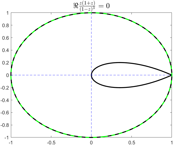
Figure 1. $u=0$

Remark 7.

In fact, when equality holds in Theorem 2 for $n=1$, we have

$$u(x,y)=\frac{-x^{5}+2x^{4}-2x^{3}y^{2}+x^{2}\left(6y^{2}-2\right)-x(y^{4}-1)+4y^{2}\left(y^{2}-1\right)}{\left(x^{2}-x+y^{2}+1\right)^{3}}.$$

The graph of $\{u=0\}$ is illustrated as above. We can see that $\{u=0\}$ almost forms a closed contour in $B_{1}(0)$, which is the equality case of Theorem 2.

Applying Bieberbach theorem directly, we can give a proof of Theorem 3.

Proof of Theorem 3. Without loss of generality, we take $d=1,p=0$ (otherwise, replace $u(z)$ by $v(z)=u(dz+p)$), and after a rotation and scaling, we set $\tilde{u}_{x}(0)=1,\tilde{u}_{y}(0)=0$, where $\tilde{u}:=\partial^{n-1}u/\partial x^{n-1}$ (note only $\tilde{u}_{x},\tilde{u}_{y}$ counts in $\nabla^{n}u$).

Since $B_{1}(0)$ is simply connected, there is an analytic function $f(z)$ defined in $B_{1}(0)$, such that $u(z)=\Re f(z)$ and $f(0)=0$. From the condition, we know that $\left|\nabla\tilde{u}\right|\neq 0$ in $B_{1}(0)$. Note

$$f^{(n)}(z)=\frac{\partial^{n}u}{\partial x^{n}}(z)-i\frac{\partial^{n}u}{\partial x^{n-1}\partial y}(z),$$

i.e. $\left|f^{(n)}(z)\right|=\left|\nabla\tilde{u}(z)\right|\neq 0$ in $B_{1}(0)$, $f^{(n-1)}(0)=0,f^{(n)}(0)=1$. So $f^{(n-1)}$ is injective and can be represented by

(2.12) $$f^{(n-1)}(z)=z+a_{2}z^{2}+a_{3}z^{3}+\cdots,$$

where $a_{2}=\frac{f^{(n+1)}(0)}{2}$. Applying Bieberbach theorem to $f^{(n-1)}$, we have $\left|a_{2}\right|\leq 2$, and $\left|a_{2}\right|=2$ holds if and only if $f^{(n-1)}(z)=\frac{z}{(1-e^{i\theta}z)^{2}}$, which are the rotated Koebe functions.

By the equation (2.6)

$$\left|\kappa(u)(0)\right| = \left|\frac{2}{n^{2}+n}\frac{\Re\left(e^{i(n+1)\theta_{k}}f^{(n+1)}(0)\right)}{\left|f^{(n)}(0)\right|}\right|\leq\frac{4}{n^{2}+n}\left|a_{2}\right|\leq\frac{8}{n^{2}+n},$$

where

$$\theta_{k}=\frac{k\pi+\frac{1}{2}\pi}{n},\quad 0\leq k\leq n-1,$$

and

$$\left|\kappa(u)(0)\right|=\frac{8}{n^{2}+n}\iff e^{i\theta}=e^{-i(n+1)\theta_{k}},\quad i.e.\ \theta=\tilde{\theta}_{k},$$

where $\tilde{\theta}_{k}$ is the same as in Theorem 2. In this case,

$$f^{(n-1)}(z)=\sum_{m=1}^{+\infty}e^{i(m-1)\tilde{\theta}_{k}}z^{m},$$

Thus, with the fact $f(0)=0$ and $\left|f^{(k)}(0)\right|=\left|\nabla\left(\frac{\partial^{k-1}u}{\partial x^{k-1}}\right)(0)\right|=0$, we have

$$f(z)=\sum_{m=1}^{+\infty}\frac{m!}{(m+n-1)!}e^{i(m-1)\tilde{\theta}_{k}}z^{m+n-1},$$

which completes the proof. $\square$

Remark 8.

For $n=1$, Theorem 3 tells us the curvature of nodal sets of harmonic functions at any non-critical point can be also bounded by the distance between the point and the nearest critical point.

Remark 9.

It seems that the condition in Theorem 3 is slightly stronger than the condition in Theorem 2. In fact, on the contrast, $u(0)=0,\nabla u\neq 0$ in $B_{1}(0)$ does not mean that $\Gamma=\{u=0\}\cap B_{1}(0)$ only has one nodal curve when $n=1$. For instance, using Riemman mapping theorem, we get a conformal function $f:B_{1}(0)\rightarrow\Omega$ with $f(0)=0$, where $\Omega$ is illustrated in figure 2.

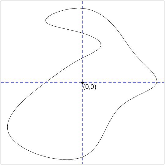
Figure 2. domain of $\Omega$

Let $u(x,y)=\Re f(x+iy)$, then $u$ has no critical points in $B_{1}(0)$ and the sign of $u$ changes four times. That is, besides the nodal curve across the origin, there is another nodal curve in $B_{1}(0)$.