CauF-VAE: Causal Disentangled Representation Learning with VAE and Causal Flows

Abstract

Disentangled representation learning aims to learn a low dimensional representation of data where each dimension corresponds to one underlying generative factor. Due to the causal relationships between generative factors in real-world situations, causal disentangled representation learning has received widespread attention. In this paper, we first propose a variant of autoregressive flows, called causal flows, which incorporate true causal structure of generative factors into the flows. Then, we design a new VAE model based on causal flows named Causal Flows Variational Autoencoders (CauF-VAE) to learn causally disentangled representations. We provide a theoretical analysis of the disentanglement identifiability of CauF-VAE by incorporating supervised information on the ground-truth factors. The performance of CauF-VAE is evaluated on both synthetic and real datasets, showing its capability of achieving causal disentanglement and performing intervention experiments. Moreover, CauF-VAE exhibits remarkable performance on downstream tasks and has the potential to learn true causal structure among factors.

1 Introduction

Representation learning aims to learn a representation of data that allows for easier extraction of useful information when constructing classifiers or other predictors [1]. Disentangled representation learning is an important step towards better representation learning. It assumes that high dimensional data is generated by low dimensional, semantically meaningful factors, called ground-truth factors. Thus, disentangled representation learning refers to learning a representation where changes in one dimension are caused by only one factor of variation in the data [2]. The common framework for obtaining disentangled representations is Variational Autoencoders (VAE) [3].

Recently, many unsupervised methods of learning disentangled representations with VAE have been proposed , mainly by imposing independent constraints on the posterior or aggregate posterior of latent variables $\mathbf{z}$ through KL divergence [4, 5, 6, 7, 8, 9, 10]. Later, authors in [2] proposed that it is almost impossible to achieve disentanglement in an unsupervised manner without inductive bias. Therefore, some weakly supervised or supervised methods were proposed[11, 12, 13, 14, 15]. However, most of them assumed that the generative factors are independent of each other, while in the real world, the generative factors of interest are likely to have causal relationships with each other. At this point, the above models can’t achieve disentanglement of causally related factors [12, 16]. In order to achieve the purpose of causal disentanglement, many state-of-the-art methods have been proposed [12, 13, 17, 18, 19].

Normalizing flows [20] are common methods for improving inference ability of VAE. By composing invertible transformations, they make the posterior distribution of VAE closer to the true posterior distribution. One of the most popular normalizing flows is autoregressive flows[21], which has been brought into VAE[22]. It has been discovered that the causal order of variables can be learned via autoregressive flows[23]. Inspired by this application, we develop causal flows that can impose true causal structure on the variables.

In this paper, we introduce causal flows that incorporate causal structure information of ground-truth factors, and propose a causal disentanglement model, called CauF-VAE, which combines VAE with causal flows to learn causally disentangled representations. After encoding the input data by VAE’s encoder and processing it through causal flows, we obtain the causally disentangled representations, which will be fed into the decoder for the reconstruction of the original image. To theoretically guarantee causal disentanglement of our model, we also include supervised information about the underlying factors. The contributions of our work are as follows:

(1) We introduce causal flows, the improved autoregressive flows that integrate true causal structure information of ground-truth factors.

(2) We propose a new VAE model, CauF-VAE, which employs the causal flows to learn causally disentangled representations.

(3) We theoretically prove that CauF-VAE satisfies disentanglement identifiability.

(4) We empirically show that CauF-VAE can achieve causal disentanglement and perform intervention experiments on both synthetic and real datasets. Our model exhibits excellent performance in terms of sampling efficiency in downstream tasks, and further experiments indicate its potential to learn true causal structure.

2 Background

2.1 Variational Autoencoders

Let $\{\mathbf{x}_{j}\}_{j=1}^{N}$ denote i.i.d training data, $\mathbf{x}\in\mathbb{R}^{n}$ be the observed variables and $\mathbf{z}\in\mathbb{R}^{d}$ be the latent variables. The dataset $\mathcal{X}$ has an empirical data distribution denoted as $q_{\mathcal{X}}$. The generative model defined over $\mathbf{x}$ and $\mathbf{z}$ is $p_{\bm{{\bm{\theta}}}}(\mathbf{x},\mathbf{z})=p(\mathbf{z})p_{\bm{\theta}}(\mathbf{x}|\mathbf{z})$, where ${\bm{\theta}}$ is the parameter of the decoder. Typically, $p(\mathbf{z})=N({\bm{0}},{\mathbf{I}})$, $p_{\bm{\theta}}(\mathbf{x}|\mathbf{z})=N(f_{\bm{\theta}}(\mathbf{z}),\sigma^{2}{\mathbf{I}})$, where $f_{\bm{\theta}}(\mathbf{z})$ is a neural network. Then, the marginal likelihood $p_{\bm{\theta}}(\mathbf{x})=\int p_{\bm{\theta}}(\mathbf{x},\mathbf{z})d\mathbf{z}$ is intractable to maximize. Therefore, VAE[3] introduces a parametric inference model $q_{\bm{\phi}}(\mathbf{z}|\mathbf{x})=N(\mu_{\bm{\phi}}(\mathbf{x}),diag(\sigma_{\bm{\phi}}^{2}(\mathbf{x}))$, also called an encoder or a recognition model, to obtain the variational lower bound on the marginal log-likelihood, i.e., the Evidence Lower BOund (ELBO):

$$\rm{ELBO}(\bm{\phi},\bm{\theta}) = \mathbb{E}_{q_{\mathcal{X}}}\left[{\rm{log}}\,p_{\bm{\theta}}(\mathbf{x})-D_{{\rm{KL}}}(q_{\bm{\phi}}(\mathbf{z}|\mathbf{x})||p_{\bm{\theta}}(\mathbf{z}|\mathbf{x}))\right]$$ (1)

$$= \mathbb{E}_{q_{\mathcal{X}}}\left[\mathbb{E}_{q_{\bm{\phi}}(\mathbf{z}|\mathbf{x})}({\rm{log}}\,p_{\bm{\theta}}(\mathbf{x},\mathbf{z})-{\rm{log}}\,q_{\bm{\phi}}(\mathbf{z}|\mathbf{x}))\right]$$

$$= \mathbb{E}_{q_{\mathcal{X}}}\left[\mathbb{E}_{q_{\bm{\phi}}(\mathbf{z}|\mathbf{x})}{\rm{log}}\,p_{\bm{\theta}}(\mathbf{x}|\mathbf{z})-D_{{\rm{KL}}}(q_{\bm{\phi}}(\mathbf{z}|\mathbf{x})||p(\mathbf{z}))\right]$$

As can be seen from equation (1), maximizing $\mathcal{L}(\mathbf{x},{\bm{\phi}},{\bm{\theta}})$ will simultaneously maximize ${\rm{log}}\,p_{\bm{\theta}}(\mathbf{x})$ and minimize $D_{{\rm{KL}}}(q_{\bm{\phi}}(\mathbf{z}|\mathbf{x})||p_{\bm{\theta}}(\mathbf{z}|\mathbf{x}))\geq 0$. Therefore, we wish $q_{\bm{\phi}}(\mathbf{z}|\mathbf{x})$ to be flexible enough to match the true posterior $p_{\bm{\theta}}(\mathbf{z}|\mathbf{x})$. At the same time, based on the third line of equation (1), which is often used as objective function of VAE, we require that $q_{\bm{\phi}}(\mathbf{z}|\mathbf{x})$ is efficiently computable, differentiable, and sampled from.

2.2 Autoregressive Normalizing Flows

Normalizing flows[20] are effective solutions to the issues mentioned above. The flows construct flexible posterior distribution through expressing $q_{\bm{\phi}}(\mathbf{z}|\mathbf{x})$ as an expressive invertible and differentiable mapping $\bm{g}$ of a random variable with a relatively simple distribution, such as an isotropic Normal. Typically, $\bm{g}$ is obtained by composing a sequence of invertible and differentiable transformations $\bm{g}_{1},\bm{g}_{2},\ldots,\bm{g}_{K}$, i.e., $\bm{g}=\bm{g}_{K}\circ\cdots\circ\bm{g}_{1},\bm{g}_{k}:\mathbb{R}^{d+n}\rightarrow\mathbb{R}^{d},\forall k=1\ldots K$. If we define the initial random variable (the output of encoder) as $\mathbf{z}_{0}$ and the final output random variable as $\mathbf{z}_{K}$, then $\mathbf{z}_{k}=\bm{g}_{k}(\mathbf{z}_{k-1},\mathbf{x}),\forall k$. In this case, we can use $\bm{g}$ to obtain the conditional probability density function of $\mathbf{z}_{K}$ by applying the general probability-transformation formula[24]:

$$q_{{\bm{\phi}}}(\mathbf{z}_{K}|\mathbf{x})=q_{\bm{\phi}}(\mathbf{z}_{0}|\mathbf{x})\left|{\rm{det}}\,J_{\bm{g}(\mathbf{z}_{0},\mathbf{x})}\right|$$ (2)

where ${\rm{det}}\,J_{\bm{g}(\mathbf{z}_{0},\mathbf{x})}$ is the Jacobian determinants of $\bm{g}$ with respect to $\mathbf{z}_{0}$.

Autoregressive flows are one of the most popular normalizing flows[21, 24]. By carefully designing the function $\bm{g}$, the Jacobian matrix in equation (2) becomes a lower triangular matrix, so the determinant can be computed in linear time. For illustration, we will only use a single-step flow with notation $\bm{g}$. Multi-layer flows are simply the composition of the function represented by a single-step flow, as mentioned earlier. And we will denote the input to the function $\bm{g}$ as $\mathbf{z}$ and its output as $\widetilde{\mathbf{z}}$. In the autoregressive flows, $\bm{g}$ has the following form:

$$\mathbf{\widetilde{z}}=\bm{g}(\mathbf{z},\mathbf{x})=\left[g^{1}(\mathbf{z}^{1};\bm{h}^{1})\ldots g^{d}(\mathbf{z}^{d};\bm{h}^{d})\right]^{\rm T}\quad{\rm{where}}\quad\bm{h}^{i}=\bm{c}^{i}(\mathbf{\widetilde{z}}^{<i},\mathbf{x})$$ (3)

where $g^{i}$, an invertible function of input $\mathbf{z}^{i}$, is termed as a transformer. Here $\mathbf{z}^{i}$ stands for the i-th element of vector $\mathbf{z}$, and $\bm{c}^{i}$ is the i-th conditioner, a function of the first $i-1$ elements of $\widetilde{\mathbf{z}}$, which determines part of parameters of the transformer $g^{i}$. We use neural networks to fit $\bm{c}$. IAF[22] improves the performance of VAE by using autoregressive flows to generate more flexible posterior distribution.

Performing causal inference tasks

The ordering of variables in autoregressive flows can be explained using the Structural Equation Models (SEMs)[23, 25], due to the similarity between equation (3) and the SEMs. A special form of autoregressive flows (affine flows) allows us to obtain a new class of causal models. Moreover, we could efficiently learn the causal direction between two variables or pairs of multivariate variables from a dataset by using autoregressive flows according to [23].

3 Causal Flows

Motivated by the connection between autoregressive flows and SEMs, we propose an extension to the autoregressive flows by incorporating an adjacency matrix $A$. The extended flows still involve functions with tractable Jacobian determinants.

In autoregressive flows, according to equations (3) and the third section in [23], causal order is established among variables $\mathbf{\widetilde{z}}^{1},\cdots,\mathbf{\widetilde{z}}^{d}$. Given the causal graph of the variables $\mathbf{\widetilde{z}}^{1},\cdots,\mathbf{\widetilde{z}}^{d}$, let $A\in\mathbb{R}^{d\times d}$ denote its corresponding weighted adjacency matrix, $A_{i,:}$ is the row vector of $A$ and $A_{i,j}$ is nonzero only if $\mathbf{{\widetilde{z}}}^{j}$ is the parent node of $\mathbf{{\widetilde{z}}}^{i}$, then $A$ corresponding to the causal order in autoregressive flows is a full lower-triangular matrix. The conditioner can be written in the form of $\bm{c}^{i}(\mathbf{\widetilde{z}}\circ A,\mathbf{x})$, where $\circ$ is the element-wise product.

The binary adjacency matrix corresponding to $A$ is $\mathbf{I}_{A}=\mathbf{I}(A\neq 0)$, here $\mathbf{I}$ is the element-wise indicator function. If we utilize prior knowledge about the true causal structure among variables, i.e., if a certain causal structure$(A$ or $\mathbf{I}_{A})$ among variables is known, then $A$ is still a lower triangular matrix, but some of its entries are set to 0 according to the underlying causal graph. We can integrate such $A$ into the conditioner, which is also denoted as $\bm{c}^{i}(\mathbf{\widetilde{z}}\circ A,\mathbf{x})$. In the following text, we will refer to it as the causal conditioner.

We define autoregressive flows that use a causal conditioner as Causal Flows. Besides the conditioner, we also need to specify the transformer to construct flows[24, 26]. The transformer can be any invertible function, and in this paper, we focus on affine transformer, which is one of the simplest transformers. At this point, causal flows $\bm{g}$ can be formulated as follows:

$$\widetilde{\mathbf{z}}^{i}=g^{i}(\mathbf{z}^{i};\bm{h}^{i})=\mathbf{z}^{i}\,{\rm{exp}}(s_{i}(\widetilde{\mathbf{z}}\circ A_{i,:},\mathbf{x}))+t_{i}(\widetilde{\mathbf{z}}\circ A_{i,:},\mathbf{x})$$ (4)

where $\bm{s}=\left[s_{1},\cdots,s_{d}\right]^{\rm{T}}\in\mathbb{R}^{d}$ and $\bm{t}=\left[t_{1},\cdots,t_{d}\right]^{\rm{T}}\in\mathbb{R}^{d}$ are defined by the conditioner, i.e., $\bm{h}^{i}=\left\{s_{i},t_{i}\right\}$, while $s_{1}$ and $t_{1}$ are constants.

Given that the derivative of the transformer with respect to $\mathbf{z}^{i}$ is ${\rm{exp}}(s_{i}(\widetilde{\mathbf{z}}\circ A_{i,:}))$ and $A$ is lower-triangular, the log absolute Jacobian determinant is:

$${\rm{log}}\,\left|{\rm{det}}\,J_{\bm{g}(\mathbf{z},\mathbf{x})}\right|=\sum_{i=1}^{d}{\rm{log}}\,{\rm{exp}}(s_{i}(\widetilde{\mathbf{z}}\circ A_{i,:},\mathbf{x}))=\sum_{i=1}^{d}s_{i}(\widetilde{\mathbf{z}}\circ A_{i,:},\mathbf{x})$$ (5)

Now, we are able to derive the log probability density function of $\widetilde{\mathbf{z}}$ using the following expression:

$${\rm log}\,q_{{\bm{\phi}}}(\widetilde{\mathbf{z}}|\mathbf{x})={\rm log}\,q_{\bm{\phi}}(\mathbf{z}|\mathbf{x})-\sum_{i=1}^{d}s_{i}(\widetilde{\mathbf{z}}\circ A_{i,:},\mathbf{x})$$ (6)

It is worth emphasizing that the computation of autoregressive flows in equation (3) needs to be performed sequentially, meaning that $\widetilde{\mathbf{z}}^{<i}$ must be calculated before $\widetilde{\mathbf{z}}^{i}$. Due to the sampling requirement in VAE, this approach may not be computationally efficient. However, in causal disentanglement applications of VAE, the number of factors of interest is often relatively small. Additionally, we’ve found that using a single layer of causal flows and lower-dimensional latent variables are enough to lead to better results, so the computational cost of the model is not significantly affected by sequential sampling.

4 CauF-VAE: Causal Flows for VAE Disentanglement

This section focuses on addressing the issue of causal disentanglement in VAE. The main approach is to introduce causal flows into VAE, since we expect that causal flows have the same ability as autoregressive flows to learn the order of variables, and further enabling VAE to learn the causal structure between its latent variables by imposing the causal structure information to the model. Moreover, we will incorporate supervised information into the model to achieve the alignment between latent variables and the ground-truth factors, ultimately achieving causal disentanglement.

First, we introduce some notations following [12]. We denote $\bm{\xi}\in\mathbb{R}^{m}$ as the underlying ground-truth factors of interest for data $\mathbf{x}$, with distribution $p_{\bm{\xi}}$. For each underlying factor $\bm{\xi}^{i}$, we denote $\bm{y}^{i}$ as some continuous or discrete annotated observation satisfying $\bm{y}^{i}={\mathbb{E}}(\bm{\xi}^{i}|\mathbf{\mathbf{x}})$, where the superscript $i$ still denotes the i-th element of each vector. Let $\mathcal{D}=\left\{(\mathbf{x}_{j},\bm{y}_{j},\mathbf{u}_{j})\right\}_{j=1}^{N}$ denotes a labeled dataset, where $\bm{u}_{j}\in\mathbb{R}^{k}$ is the additional observed variable. Depending on the context, the variable $\mathbf{u}$ can take on various meanings, such as serving as the time index in a time series, a class label, or another variable that is observed concurrently [27]. We get $\bm{y}^{i}={\mathbb{E}}(\bm{\xi}^{i}|\mathbf{\mathbf{x}},\mathbf{u})$, where $i=1,\cdots,m$. This is because if $\mathbf{u}$ is ground-truth factor $\bm{y}$, it is obviously true, otherwise, $\bm{y}^{i}={\mathbb{E}}(\bm{\xi}^{i}|\mathbf{\mathbf{x}},\mathbf{u})={\mathbb{E}}(\bm{\xi}^{i}|\mathbf{\mathbf{x}})$. We will view the encoder and flows as an unified stochastic transformation $E$, with the learned representation $\widetilde{\mathbf{z}}$ as its final output, i.e., $\widetilde{\mathbf{z}}=E(\mathbf{x},\mathbf{u})$. Additionally, in the stochastic transformation $E(\mathbf{x},\mathbf{u})$, we use $\bar{E}(\mathbf{x},\mathbf{u})$ to denote its deterministic part, i.e., $\bar{E}(\mathbf{x},\mathbf{u})=\mathbb{E}(E(\mathbf{x},\mathbf{u})|\mathbf{x},\mathbf{u})$.

Now, we adopt the definition of causal disentanglement as follows:

Definition 1 (Disentangled representation[12])

Considering the underlying factor $\bm{\xi}\in\mathbb{R}^{m}$ of data $\mathbf{x}$, $E$ is said to learn a disentangled representation with respect to $\bm{\xi}$ if there exists a one-to-one function $r_{i}$ such that ${{\bar{E}}(\mathbf{x},\mathbf{u})}^{i}=r_{i}(\bm{\xi}^{i}),\forall i=1,\cdots,m$.

As noted in [12], the purpose of this definition is to guarantee some degree of alignment between the latent variable $E(\mathbf{x})$ and the underlying factor $\bm{\xi}$ in the model. In our approach, we will also supervise each latent variable with label for each underlying factor, thus establishing such component-wise relationship between them.

4.1 CauF-VAE

To learn a disentangled representation that meets the definition mentioned above, we proceed to present the full probabilistic form of CauF-VAE.

We define the inference model (see Figure 1) that utilizes causal flows as follows:

$$q_{{\bm{\phi}}}(\mathbf{z}|\mathbf{x},\mathbf{u}) = q_{{\bm{\epsilon}}}(\mathbf{z}-{\bm{\phi}}(\mathbf{x},\mathbf{u}))$$ (7)

$$\mathbf{z} \sim q_{{\bm{\phi}}}(\mathbf{z}|\mathbf{x},\mathbf{u})$$ (8)

$$\widetilde{\mathbf{z}} = \bm{g}(\mathbf{z},\mathbf{x})$$ (9)

$$q_{{\bm{\phi}},{\bm{\gamma}}}(\widetilde{\mathbf{z}}|\mathbf{x},\mathbf{u}) = q_{\bm{\phi}}(\mathbf{z}|\mathbf{x},\mathbf{u})\prod\limits_{i=1}^{d}{\rm exp}(-s_{i}(\widetilde{\mathbf{z}}\circ A_{i,:},\mathbf{x}))$$ (10)

where we use ${\bm{\gamma}}=(\bm{s},\bm{t},A)\in\bm{\Gamma}$ to denote parameters of causal flows. Equation (7) indicates that $\mathbf{z}=\bm{\phi}(\mathbf{x},\mathbf{u})+\bm{\epsilon}$, where the probability density of ${\bm{\epsilon}}$ is $q_{\bm{\epsilon}}(\bm{\epsilon})=\mathcal{N}(\bm{0},{\mathbf{I}})$ and $\bm{\phi}(\mathbf{x},\mathbf{u})$ denotes the encoder. Equation (8) and (9) describe the process of transforming the original encoder output $\mathbf{z}$ into the final latent variable representation $\widetilde{\mathbf{z}}$ by using causal flows. Eventually, the posterior distribution obtained by the inference model is represented by equation (10). Now, the parameters of stochastic transformation $E(\mathbf{x},\mathbf{u})$ are $\bm{\phi}$ and ${\bm{\gamma}}$.

Then, the conditional generative model is defined as follows:

$$p_{\bm{{\theta}}}(\mathbf{x},\widetilde{\mathbf{z}}|\mathbf{u}) = p_{\mathbf{f}}(\mathbf{x}|\widetilde{\mathbf{z}},\mathbf{u})p_{\mathbf{T},\bm{\lambda}}(\widetilde{\mathbf{z}}|\mathbf{u})$$ (11)

$$p_{\mathbf{f}}(\mathbf{x}|\widetilde{\mathbf{z}},\mathbf{u}) = p_{\mathbf{f}}(\mathbf{x}|\widetilde{\mathbf{z}})\quad=\quad p_{\bm{\zeta}}(\mathbf{x}-\mathbf{f}(\widetilde{\mathbf{z}}))$$ (12)

$$p_{\mathbf{T},\bm{\lambda}}(\widetilde{\mathbf{z}}|\mathbf{u})=\begin{cases}\frac{Q(\widetilde{\mathbf{z}}^{\leq m})e^{<\mathbf{T}(\widetilde{\mathbf{z}}^{\leq m}),\bm{\lambda}(\mathbf{u})>}}{Z(\mathbf{u})}\\ \mathcal{N}(\bm{0}_{(d-m)\times 1},\mathbf{I}_{(d-m)\times(d-m)})\end{cases}$$ (13)

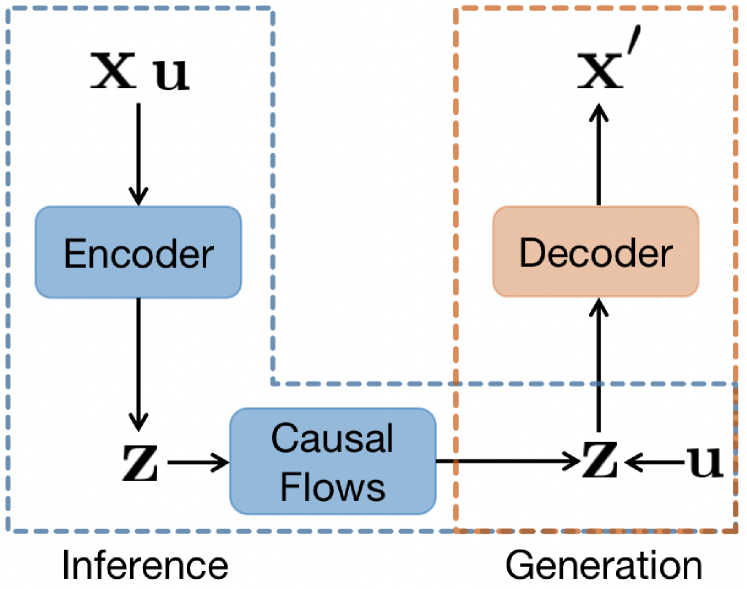
Figure 1: Model structure of
CauF-VAE.

where $\bm{\theta}=(\mathbf{f},\mathbf{T},\bm{\lambda})\in\bm{\Theta}$ are model parameters. Equation (11) describes the process of generating $\mathbf{x}$ from $\mathbf{z}$. Equation (12) indicates that $\mathbf{x}=\mathbf{f}(\widetilde{\mathbf{z}})+\bm{\zeta}$, where $p_{\bm{\zeta}}({\bm{\zeta}})=\mathcal{N}(\bm{0},{\mathbf{I}})$ and the decoder $\mathbf{f}(\widetilde{\mathbf{z}})$ is assumed to be an invertible function, which is approximated by a neural network. As presented in equation (13), we use the exponential conditional distribution[28] for the first $m$ dimensions and another distribution (e.g., standard normal distribution) for the remaining $d-m$ dimensions to capture other non-interest factors for generation[12], where $\mathbf{T}:{\mathbb{R}}^{d}\rightarrow{\mathbb{R}}^{d\times l}$ is the sufficient statistic, ${\bm{\lambda}}:{\mathbb{R}}^{k}\rightarrow{\mathbb{R}}^{d\times l}$ is the corresponding parameter, $Q:{\mathbb{R}}^{d}\rightarrow{\mathbb{R}}$ is the base measure, $Z(\mathbf{u})$ is the normalizing constant and $<\cdot,\cdot>$ denotes the dot product. If $d=m$, we will only use the conditional prior in the first line of (13). We present the model structure of CauF-VAE in Figure 1.

The prior distribution will no longer be a factorial distribution after adding information $\mathbf{u}$, thus it can better reflect the actual situation. Additionally, when we have labels $\bm{y}$ or use $\mathbf{u}$ to represent the labels, we can add a regularization term in the objective function to promote the consistency between $\bm{\xi}$ and $E(\mathbf{x})$[11, 12]. Now we suppose that the dataset $\mathcal{X}$ has an empirical data distribution denoted by $q_{\mathcal{X}}(\mathbf{x},\mathbf{u})$. Our goal turns into maximizing the variational lower bound on the marginal likelihood $p_{\bm{\theta}}(\mathbf{x}|\mathbf{u})$. Therefore, the loss function of CauF-VAE is formulated as follows:

$$\mathcal{L}(\bm{\phi},\bm{\gamma},\bm{\theta}) = -{\rm{ELBO}}(\bm{\phi,\gamma,\theta})+\beta_{sup}\mathcal{L}_{sup}(\bm{\phi},\bm{\gamma})$$ (14)

$$= \mathbb{E}_{q_{\mathcal{X}}}\left[\mathbb{E}_{q_{{\bm{\phi}},{\bm{\gamma}}}(\widetilde{\mathbf{z}}|\mathbf{x},\mathbf{u})}{\rm{log}}\,p_{\mathbf{f}}(\mathbf{x}|\widetilde{\mathbf{z}},\mathbf{u})-D_{{\rm{KL}}}(q_{{\bm{\phi}},{\bm{\gamma}}}(\widetilde{\mathbf{z}}|\mathbf{x},\mathbf{u})||p_{\mathbf{T},\bm{\lambda}}(\widetilde{\mathbf{z}}|\mathbf{u}))\right]$$

$$+\quad\beta_{sup}{\mathbb{E}}_{(\mathbf{x},\bm{y},\mathbf{u})}\left[l_{sup}(\bm{\phi},\bm{\gamma})\right]$$

where $\beta_{sup}\textgreater 0$ is a hyperparameter, $l_{sup}(\bm{\phi},\bm{\gamma})=\sum_{i=1}^{m}-\bm{y}^{i}{\rm log}\,\sigma({\bar{E}}(\mathbf{x},\mathbf{u})^{i})-(1-\bm{y}^{i}){\rm log}\,(1-\sigma({\bar{E}}(\mathbf{x},\mathbf{u})^{i}))$ is the cross-entropy loss if ${\bm{y}}^{i}$ is the binary label, and $l_{sup}(\bm{\phi},\bm{\gamma})=\sum_{i=1}^{m}(\bm{y}^{i}-{\bar{E}}(\mathbf{x},\mathbf{u})^{i})^{2}$ is the Mean Squared Error (MSE) if ${\bm{y}}^{i}$ is the continuous observation. The loss term $\mathcal{L}_{sup}$ aligns the factor of interest $\bm{\xi}\in\mathbb{R}^{m}$ with the first $m$ dimensions of the latent variable $\mathbf{z}$, which is a technique proposed in [12, 15] to satisfy the Definition 1.

Disentanglement Identifiability Analysis

Following the approach in [12], we establish the identifiability of disentanglement of CauF-VAE, which confirms that our model can learn disentangled representations. As we only focus on disentangling the factors of interest, we will, for simplicity, present our proposition in the case where $d=m$. We refer to the properties of the exponential family in the Appendix A.1[28, 29], which are used in the proof of the proposition.

Proposition 1

Under the assumptions of infinite capacity for $E$ and $\mathbf{f}$, the solution $(\bm{\phi}^{*},\bm{\gamma}^{*},\bm{\theta}^{*})\in{\rm argmin}_{\bm{\phi},\bm{\gamma},\bm{\theta}}\mathcal{L}(\bm{\phi},\bm{\gamma},\bm{\theta})$ of the loss function (14) guarantees that ${\bar{E}}_{\bm{\phi}^{*},\bm{\gamma}^{*}}(\mathbf{x})$ is disentangled with respect to $\xi$, as defined in Definition 1.

Proof See Appendix A.2.

In Proposition 1, we consider the deterministic part of the posterior distribution as the learned representation, to demonstrate the disentanglement identifiability of CauF-VAE.

Our model utilizes two types of supervised information: extra information $\mathbf{u}$ and the labels $\bm{y}$ of the ground-truth factors. In our experiments, we set $\mathbf{u}$ to be the same as $\bm{y}$, so that we only need to use one type of supervised information. With the help of the supervised information, we achieve disentanglement identifiability by using the conditional prior and additional regularization terms, which further guarantees that $\widetilde{\mathbf{z}}^{i}$ is a causal disentangled representation, for $1\leq i\leq m$. This means that the latent variables can capture the true underlying factors successfully.

5 Related Work

Causally disentangled representation learning based on VAE

Recently, achieving causally disentangled representations by VAE has received wide attention[18]. The disentangled causal mechanisms investigated in [17] and [18] assumed that the underlying factors were conditionally independent given a shared confounder. Our proposed model, in contrast, considers more general scenarios where the generative factors can exhibit more complex causal relationships. CausalVAE[13] designed an structural causal model (SCM) layer to model the causally generative mechanisms of data. DEAR[12] used a SCM to construct prior distribution, and employs Generative Adversarial Networks (GAN) to train the model. Unlike SCM-based methods, we leverage the intrinsic properties of flow models to achieve disentanglement and do not rely on external algorithms for training.

It has been proposed that causal relationships from latent variables to the reconstructed images may not hold due to the entangled structure of decoder[19]. So a disentangled decoder needs to be trained. We believe that our model can generate images sampled from the interventional distributions, which can satisfy practical needs. Moreover, we focus on representation learning, so the disentangled representations output by the encoder should be given more consideration.

Causal structure in flows

We could efficiently learn the causal direction between two variables by using autoregressive flows. Motivated by this application, we design causal flows. In a separate parallel work, authors of [30] proposed a generalized graphical normalizing flows. Similar to our design, they also utilized a conditioner that incorporated an adjacency matrix. However, their work differs from ours as we focus on developing the causal conditioner to incorporate causal structure knowledge into flows for achieving causally disentangled representation in VAE. Instead, they explored the relationship between different flows from Bayesian network perspective and designed a graph conditioner primarily for better density estimation.

6 Experiments

We empirically evaluate CauF-VAE, and demonstrate that the learned representations are causally disentangled, enabling the model to perform well on various tasks. Our experiments are conducted on both synthetic dataset and real human face image dataset, and we compare CauF-VAE with some state-of-the-art VAE-based disentanglement methods.

6.1 Experimental setup

We utilize the same datasets as [12] where the underlying generative factors are causally related. The synthetic dataset is Pendulum[13], with labels and causal graph of the factors shown in Figure 2(a). The labels are all continuous. The training and testing sets consist of 5847 and 1461 samples, respectively. The real human face dataset is CelebA[31], with 40 discrete labels. We consider two sets of causally related factors named CelebA(Attractive) and CelebA(Smile) with causal graphs also depicted in Figure 2(b) and 2(c). The training and testing sets consist of 162770 and 19962 samples, respectively.

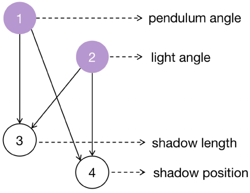
(a) Pendulum

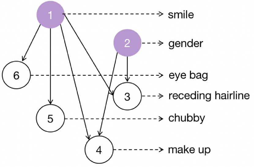
(b) CelebA(Attractive)

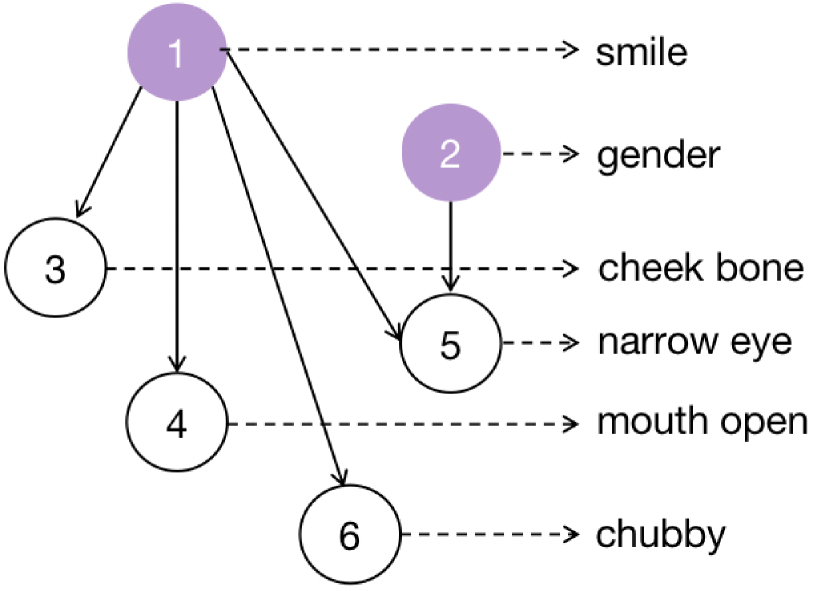
(c) CelebA(Smile)

Figure 2: Causal graphs of Pendulum and CelebA. The colored circles represent the causal variables in the graphs. In Figures (a), (b), and (c), we label the underlying factors we are interested in each dataset.

We compare our method with several representative VAE-based models for disentanglement[2], including $\beta$-VAE[4], $\beta$-TCVAE[7], and DEAR[12]. We also compare with vanilla VAE[3]. To ensure a fair comparison with equal amounts of supervised information, for each of these methods we use the same conditional prior and loss term as in CauF-VAE. For comprehensive implementation details and hyperparameters, please refer to the Appendix B.

6.2 Experimental Results

Causally Disentangled Representation

To verify that CauF-VAE indeed learns causally disentangled representations, we conduct intervention experiments. Intervention experiments involve performing the "do-operation" in causal inference[32], which allows us to visually observe the causal disentanglement of representations. Taking a single-step causal flow as an example, we demonstrate step by step how our model performs "do-operation". First, given a trained model, we input the sample $\mathbf{x}$ into the encoder, obtaining an output $\mathbf{z}$. Assuming we wish to perform the "do-operation" on $\widetilde{\mathbf{z}}^{i}$, i.e., $do(\widetilde{\mathbf{z}}^{i}=c)$, we follow the approach in [23] by treating equation (4) as SEMs. Specifically, we set the input and output of $\widetilde{\mathbf{z}}^{i}$ to the control value $c$, while other values are computed iteratively from input to output. Finally, the resulting $\widetilde{\mathbf{z}}$ is decoded to generate the desired image, which corresponds to generating images from the interventional distribution of factor $\widetilde{\mathbf{z}}$.

We perform intervention experiments by applying the "do-operation" to $m-1$ variables in the first $m$ dimensions of the latent variables, resulting in the change of only one variable. This operation, which has been referred to as "traverse", aims to test the disentanglement of our model [12]. Figures 3 and 4 show the experimental results of the CauF-VAE and DEAR on Pendulum and CelebA(Smile). We observe that when traversing a latent variable dimension, CauF-VAE has almost only one factor changing, while DEAR has multiple factors changing. This is clearly shown by comparing "traverse" results of the third row for shadow length in Figures 3(a) and 3(b), as well as the second row for gender in Figures 4(a) and 4(b). Therefore, our model can better achieve causal disentanglement.

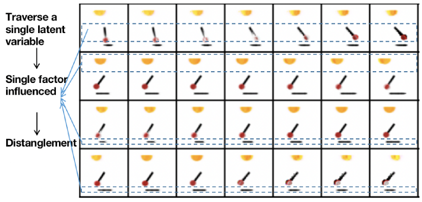
(a) Traverse of CauF-VAE

(b) Traverse of DEAR

Figure 3: Results of traverse experiments on Pendulum. Each row corresponds to a variable that we traverse on, specifically, pendulum angle, light angle, shadow length, and shadow position.

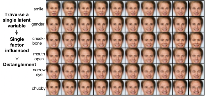
(a) Traverse of CauF-VAE

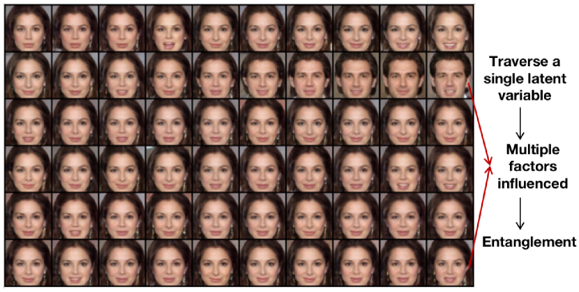
(b) Traverse of DEAR

Figure 4: Results of traverse experiments on CelebA(Smile). Each row corresponds to a variable that we traverse on, specifically, smile, gender, cheek bone, mouth open, narrow eye and chubby.

To demonstrate that our model is capable of performing interventions hence generating new images that do not exist in the dataset, we perform "do-operation" on individual latent variable. As shown in Figure 5, each row corresponds to a "do-operation" on a single dimension. In Figure 5(a), we observe that intervening on the pendulum angle and light angle causes changes in shadow length based on physical principles, but intervening on shadow length has little effect on either of these two factors. Similarly, as shown in Figure 5(b), intervening on gender affects narrow eye, but not vice versa. This demonstrates that intervening on the cause factor influences the effect factor, but not the other way around. This reflects that our latent variables have learned the true causal structure among factors to some extent, which may be attributed to the design of the causal flows with the inclusion of $A$. With $A$, we are able to leverage the causal structure among underlying factors to enable the VAE to learn the posterior distribution of the ground-truth factors and achieve causal disentanglement. More traverse and intervention results are shown in the Appendix C.

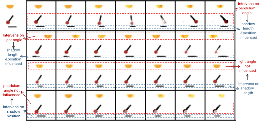
(a) Intervene factors of Pendulum

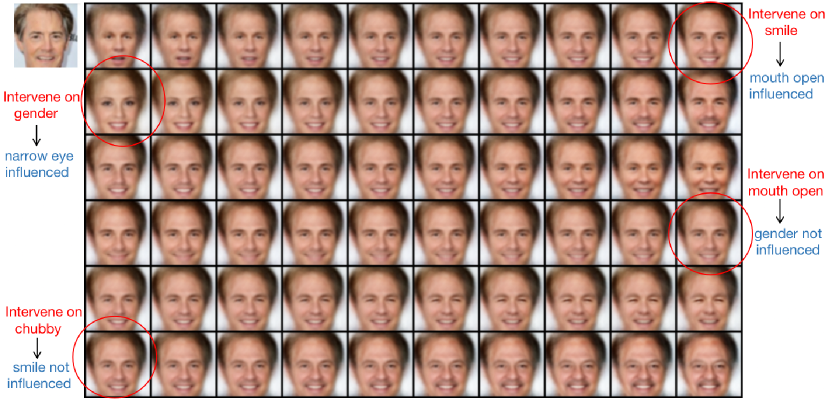
(b) Intervene factors of CelebA(Smile)

Figure 5: Results of intervention on only one variable for both Pendulum and CelebA(Smile). The image in the upper left corner of (a) and (b) are the test data we consider respectively.

Downstream task

To further illustrate benefits of causal disentangled representation, we consider its impact on a downstream task in terms of sample efficiency. A common downstream task is classification, thus we choose two classification tasks to compare our model with baseline models. Firstly, for Pendulum, we normalize factors to $\left[-1,1\right]$ during preprocessing. Then, we manually create a classification task: if $pendulum\,angle\textgreater 0$ and $light\,angle\textgreater 0$, the target label $y=1$; otherwise, $y=0$. This represents a positive class if both the pendulum and light are on the right side and a negative class otherwise. For the CelebA(Attractive) dataset, we adopt the same classification task as in [12].

We employ a MLP to train classification models, where both the training and testing sets consist of the latent variable representation $\widetilde{\mathbf{z}}$, as well as their corresponding labels $\mathbf{y}$. We adopt the statistical efficiency score defined in [2] and [12] as a measure of sample efficiency, which is defined as the classification accuracy of 100 test samples divided by the number of all (Pendulum)/10,000 test samples (CelebA). The experimental results are presented in Table 1.

Table 1: Test accuracy and sample efficiency of different models on Pendulum and CelebA datasets. Mean$\pm$standard deviations are included in the Table.

	Pendulum			CelebA
Model	100(%)	All(%)	Sample Eff	100(%)	10000(%)	Sample Eff
CauF-VAE	$\bm{99.00_{\pm 0}}$	$99.43_{\pm 0.34}$	$\bm{99.57_{\pm 0.34}}$	$\bm{81.00_{\pm 1.73}}$	$\bm{81.54_{\pm 1.76}}$	$\bm{99.34_{\pm 0.27}}$
DEAR	$88.00_{\pm 0}$	$88.55_{\pm 0.04}$	$98.63_{\pm 1.33}$	$61.00_{\pm 3.60}$	$68.50_{\pm 0}$	$89.05_{\pm 5.26}$
$\beta$-VAE	$98.67_{\pm 1.15}$	$\bm{99.59_{\pm 0.07}}$	$98.94_{\pm 0.92}$	$62.33_{\pm 5.69}$	$68.49_{\pm 0.02}$	$91.01_{\pm 8.28}$
$\beta$-TCVAE	$97.67_{\pm 1.15}$	$99.38_{\pm 0.48}$	$98.27_{\pm 0.79}$	$75.33_{\pm 3.21}$	$78.72_{\pm 4.93}$	$95.83_{\pm 4.10}$
VAE	$98.33_{\pm 0.58}$	$99.48_{\pm 0.39}$	$98.72_{\pm 0.37}$	$60.33_{\pm 2.89}$	$68.50_{\pm 0}$	$88.08_{\pm 4.21}$

Table 1 shows that CauF-VAE achieves the best sample efficiency and test accuracy on both datasets, except for the test accuracy of all test samples of Pendulum where $\beta$-VAE is the best. However, on the complex CelebA dataset, CauF-VAE significantly outperforms $\beta$-VAE. Among the baseline models, none stand out and all perform worse than CauF-VAE. It is worth noting that the encoder structures of baseline models are identical, except for DEAR, which uses ResNet as the encoder but also exhibits strong learning capacity. Therefore, we attribute the superiority of our model to our modeling approach, i.e., leveraging the fitting ability of flows, especially causal flows that greatly enhance the encoder’s ability to learn semantically meaningful representations.

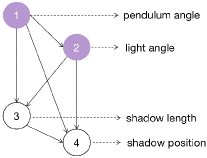
Figure 6: Super-graph of Pendulum.

Apart from the aforementioned applications, CauF-VAE has the potential to learn true causal relationships between factors, even without using a SCM[13, 33]. As shown in Figure 7(a)-7(d), for Pendulum, when our model $A$ adopts the super-graph shown in Figure 6, though the corresponding $A$ is initialized randomly around 0, it gradually approaches the true causal structure during the training process. If we set a threshold of 0.2, i.e., considering edges in causal graph smaller than the threshold as non-existing, we can obtain Figure 7(e), whose weighted matrix corresponds to the true causal structure. For details, see Appendix C.

(a) Original $A$

(b) After 20 epochs

(c) After 50 epochs

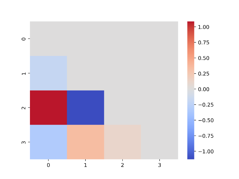
(d) After 80 epochs

(e) Final $A$

Figure 7: The learned weighted adjacency matrix $A$ given a super-graph on Pendulum. (a)-(d) illustrate the changes in $A$ as the training progresses. (e) represents $A$ after threshold processing.

We also use MIC (Maximal Information Coefficient) and TIC (Total Information Coefficient)[13, 34] to measure the strength of association between learned representations and ground-truth factors. We use all the testing data to obtain MIC and TIC. As Table 2 shows, CauF-VAE outperforms others on the pendulum dataset, while on CelebA, CauF-VAE and $\beta$-TCVAE perform comparably. This indicates that our learning representations achieve almost optimal correlation with the ground-truth factors compared to other baseline models, further validating the effectiveness of our model. Although $\beta$-TCVAE exhibits good performance, traverse experiments in Appendix C suggest that it’s possible for one latent variable to contain multiple factors information, thus resulting in outcomes with high correlation with multiple factors simultaneously.

Table 2: MIC and TIC between ground-truth factors and latent variable representations obtained by different models on three datasets.

	Pendulum		CelebA(Attractive)		CelebA(Smile)
Model	MIC	TIC	MIC	TIC	MIC	TIC
CauF-VAE	$\bm{93.27}$	$\bm{89.90}$	$\bm{42.38}$	$\bm{42.09}$	$\bm{58.53}$	$\bm{58.60}$
DEAR	$32.90$	$30.55$	$34.73$	$34.31$	$52.59$	$52.95$
$\beta$-VAE	$41.57$	$35.22$	$15.61$	$15.81$	$33.80$	$33.65$
$\beta$-TCVAE	$86.18$	$82.18$	$\bm{43.47}$	$\bm{43.36}$	$\bm{59.30}$	$\bm{58.96}$
VAE	$60.78$	$55.09$	$27.40$	$27.33$	$35.79$	$35.70$

7 Conclusion

This paper focuses on learning causally disentangled representations where the underlying generative factors are causally related. We introduce causal flows that incorporate causal structure information of factors, and propose CauF-VAE, a new VAE model that employs causal flows. By using the additional information of $\mathbf{u}$ and $\mathbf{y}$, which can both take on the labels of the ground-truth factors, the model achieves disentanglement identifiability. Experiments conducted on both synthetic and real datasets show that CauF-VAE can achieve causal disentanglement and perform intervention experiments. Furthermore, CauF-VAE exhibits excellent performance in downstream tasks and the potential to learn the causal structure. To the best knowledge of the authors, our approach is the first to achieve causal disentanglement without relying on SCM, while also not restricting the causal graphs of factors, thereby suggesting a promising research direction in this field. Semi-supervised or unsupervised models that can achieve disentanglement identifiability can be left to future work.

Acknowledgements

This research is supported by the National Nature Science Foundation of China under Grant 12071428 and 62111530247, and the Zhejiang Provincial Natural Science Foundation of China under Grant LZ20A010002.

$$\rm{Supplementary\,Material\,for}$$

$$\mathbf{CauF\mbox{-}VAE\colon Causal\,Disentangled\,Representation\,Learning}$$

$$\mathbf{with\,VAE\,and\,Causal\,Flows}$$

A Theory

We first present the properties of the exponential family distribution. Then we provide the proof for Proposition 1.

A.1 Exponential family distributions

Definition 2 (Exponential family)

A probability distribution belongs to the exponential family if its density has the following form:

$$p(\mathbf{x}|\bm{\theta})=\frac{Q(\mathbf{x})e^{<\mathbf{T}(\mathbf{x}),\bm{\lambda}(\bm{\theta})>}}{Z(\bm{\theta})}$$ (15)

where $\mathbf{x}\in\mathcal{X}$ and $\bm{\theta}\in\Theta$, $\mathbf{T}:\mathcal{X}\rightarrow{\mathbb{R}}^{k}$ is the sufficient statistic, ${\bm{\lambda}}:\Theta\rightarrow{\mathbb{R}}^{k}$ is the corresponding parameter, $Q:\mathcal{X}\rightarrow{\mathbb{R}}$ is the base measure (Lebesgue measure), $Z(\bm{\theta})$ is the normalizing constant and $<\cdot,\cdot>$ stands for the dot product. More precisely, we can refer to equation (15) as conditional exponential family[28].

Theorem 1 (Universal approximation capability)

Let $p(\mathbf{x}|\bm{\theta})$ be a conditional probability density function. Assume that $\mathcal{X}$ and $\Theta$ are compact Hausdorff spaces, and that $p(\mathbf{x}|\bm{\theta})\textgreater 0$ almost surely $\forall(\mathbf{x},\bm{\theta})\in\mathcal{X}\times\Theta$. Then for each $\epsilon\textgreater 0$, there exists $(\bm{\phi},k)\in\Phi\times\mathbb{N},\bm{\phi}=(\mathbf{T},\bm{\lambda})$, where $k$ is the dimension of the feature extractor, such that ${\rm{sup}}_{(\mathbf{x},\bm{\theta})\in\mathcal{X}\times\Theta}\left|p_{\bm{\theta}}(\mathbf{x}|\bm{\theta})-p(\mathbf{x}|\bm{\theta})\right|\textless\epsilon$.

Authors in [29] provide the above Theorem that shows the universal approximation capability of conditional exponential family. Specifically, they show that for compact Hausdorff spaces $\mathcal{X}$ and $\Theta$, any conditional probability density $p(\mathbf{x}|\bm{\theta})$ can be approximated arbitrarily well. Thus, through the consideration of a freely varying $k$, and general $\mathbf{T}$ and $\bm{\lambda}$, the conditional exponential family is endowed with universal approximation capability over the set of conditional probability densities. In practice, it is possible to achieve almost perfect approximation by choosing $k$ greater than the input dimension. However, this result does not take into account the practicality of fitting the approximation family to data, and increasing $k$ may make it more difficult to fit the data distribution in real-world scenarios.

A.2 Proof of Proposition 1

Proposition 1

Under the assumptions of infinite capacity for $E$ and $\mathbf{f}$, the solution $(\bm{\phi}^{*},\bm{\gamma}^{*},\bm{\theta}^{*})\in{\rm argmin}_{\bm{\phi},\bm{\gamma},\bm{\theta}}\mathcal{L}(\bm{\phi},\bm{\gamma},\bm{\theta})$ of the loss function (14) guarantees that ${\bar{E}}_{\bm{\phi}^{*},\bm{\gamma}^{*}}(\mathbf{x})$ is disentangled with respect to $\xi$, as defined in Definition 1.

Proof Following the approach in [12], we give a proof of this proposition. We suppose that $d=m$. For $\forall\,i=1,2,...,m$, we consider two cases separately. In the first case, $\mathcal{L}_{sup,i}(\bm{\phi},\bm{\gamma})$ is cross-entropy loss:

$$\mathcal{L}_{sup,i}(\bm{\phi},\bm{\gamma}) = \mathbb{E}_{(\mathbf{x},\mathbf{y},\mathbf{u})}\left[-\bm{y}^{i}{\rm log}\,\sigma({\bar{E}}(\mathbf{x},\mathbf{u})^{i})-(1-\bm{y}^{i}){\rm log}\,(1-\sigma({\bar{E}}(\mathbf{x},\mathbf{u})^{i}))\right]$$ (16)

$$= -\int q(\mathbf{x},\mathbf{u})p(\bm{y}^{i}|\mathbf{x},\mathbf{u})[\bm{y}^{i}{\rm log}\,\sigma({\bar{E}}(\mathbf{x},\mathbf{u})^{i})$$

$$+(1-\bm{y}^{i}){\rm log}\,(1-\sigma({\bar{E}}(\mathbf{x},\mathbf{u})^{i}))]d\mathbf{x}d\mathbf{u}d\bm{\xi}^{i}$$

where $P(\bm{y}^{i}=1|\mathbf{x},\mathbf{u})=\mathbb{E}(\bm{\xi}^{i}|\mathbf{x},\mathbf{u})$, $P(\bm{y}^{i}=0|\mathbf{x},\mathbf{u})=1-\mathbb{E}(\bm{\xi}^{i}|\mathbf{x},\mathbf{u})$. Let $\frac{\partial\mathcal{L}_{sup,i}(\bm{\phi},\bm{\gamma})}{\partial\sigma({\bar{E}}(\mathbf{x},\mathbf{u})^{i})}=0$, we know that ${\bar{E}}^{*}(\mathbf{x},\mathbf{u})^{i}=\sigma^{-1}(\mathbb{E}(\bm{\xi}^{i}|\mathbf{x},\mathbf{u}))=\sigma^{-1}(\bm{y}^{i})$ can minimize $\mathcal{L}_{sup,i}(\bm{\phi},\bm{\gamma})$.

In the second case, $\mathcal{L}_{sup,i}(\bm{\phi},\bm{\gamma})$ is Mean Squared Error (MSE):

$$\mathcal{L}_{sup,i}(\bm{\phi},\bm{\gamma})=\mathbb{E}_{(\mathbf{x},\mathbf{y},\mathbf{u})}\left[(\bm{y}^{i}-{\bar{E}}(\mathbf{x},\mathbf{u})^{i})^{2}\right]=\int q(\mathbf{x},\mathbf{u})p(\bm{y}^{i}|\mathbf{x},\mathbf{u})(\bm{y}^{i}-{\bar{E}}(\mathbf{x},\mathbf{u})^{i})^{2}d\mathbf{x}d\mathbf{u}d\bm{\xi}^{i}$$ (17)

Let $\frac{\partial\mathcal{L}_{sup,i}(\bm{\phi},\bm{\gamma})}{\partial\sigma({\bar{E}}(\mathbf{x},\mathbf{u})^{i})}=0$, we know that ${\bar{E}}^{*}(\mathbf{x},\mathbf{u})^{i}=\mathbb{E}(\bm{\xi}^{i}|\mathbf{x},\mathbf{u})=\bm{y}^{i}$ can minimize the $\mathcal{L}_{sup,i}(\bm{\phi},\bm{\gamma})$.

Next, because of the infinite capacity of $\mathbf{f}$ and Theorem 1, we know that $q_{{\bm{\phi}^{*}},{\bm{\gamma}^{*}}}(\mathbf{x},\widetilde{\mathbf{z}}|\mathbf{u})$ is contained within the distribution family of $p_{\bm{{\theta}}}(\mathbf{x},\widetilde{\mathbf{z}}|\mathbf{u})$. Then by minimizing the loss in (14) over $\bm{\theta}$, we can find $\bm{\theta}^{*}$ such that $p_{\bm{\theta}^{*}}(\mathbf{x},\widetilde{\mathbf{z}}|\mathbf{u})$ matches $q_{{\bm{\phi}^{*}},{\bm{\gamma}^{*}}}(\mathbf{x},\widetilde{\mathbf{z}}|\mathbf{u})$ and thus

$$-{\rm{ELBO}}(\bm{\phi^{*},\gamma^{*},\theta^{*}})=D_{{\rm{KL}}}(q_{{\bm{\phi}^{*}},{\bm{\gamma}^{*}}}(\mathbf{x},\widetilde{\mathbf{z}}|\mathbf{u})||p_{\bm{\theta}^{*}}(\mathbf{x},\widetilde{\mathbf{z}}|\mathbf{u}))+\rm{constant}$$ (18)

reaches minimum.

Therefore, by minimizing the loss function (14) of CauF-VAE, we can get the solution, that is, ${{\bar{E}}^{*}(\mathbf{x},\mathbf{u})}^{i}=r_{i}(\bm{\xi}^{i})$ with $r_{i}(\bm{\xi}^{i})=\sigma^{-1}(\bm{\xi}^{i})$ if cross-entropy loss is used, and $r_{i}(\bm{\xi}^{i})=\bm{\xi}^{i}$ if MSE is used. Here, $\mathbf{x}$ denotes random variable.

To sum up, ${\bar{E}}_{\bm{\phi}^{*},\bm{\gamma}^{*}}(\mathbf{x},\mathbf{u})$ is disentangled with respect to $\xi$, as defined in Definition 1.

B Experimental Details

We present the main settings used in our experiments. Our experiments on Pendulum utilize one NVIDIA GeForce RTX 2080ti GPU, while experiments on CelebA use one NVIDIA GeForce RTX 3080 GPU. To train DEAR, we use two NVIDIA GeForce RTX 2080ti GPUs.

B.1 Data preprocessing

Pendulum

We generate the pendulum dataset using the synthetic simulators mentioned in [12] and [13]. For detailed generation procedures, please refer to Appendix F in [12] or Appendix C.1.1 in [13]. The pendulum images are resized to 64×64×3 resolution, and the training and testing sets consist of 5847 and 1461 samples, respectively.

CelebA

We employ the default training and testing sets in CelebA, with 162770 and 19962 samples, respectively. We also resize the images to 64×64×3 resolution. We set the values of features that are $-$1 to 0.

B.2 Experimental setup

Causal Flows Implementation

In CauF-VAE, we incorporate causal flows to enhance the model’s ability to capture causal underlying factors. As discussed in Section 2.2, complex composite functions can be obtained by composing multiple simple transformations, which is the main mechanism adopted by flow models. However, in order to preserve the causal relationships between variables in the output representation and to verify the ability of the causal flows, we only use a single layer of causal flow in our experiments. As Proposition 1 shows, the $mean$ of the output latent variables from the causal flow can achieve disentanglement. In practice, finding the exact value of the $mean$ can be challenging, so we use random sampling to approximate it by drawing $N$ samples. In our experiments, we set $N$ to be 1. In causal flows, besides the affine transformation introduced in Section 3, other implementation methods such as integration-based transformers[26] can also be used, but the computational cost for sampling or density estimation needs to be taken into consideration when modeling.

Conditional prior Implementation

Regarding the setting of conditional prior, since it is generally difficult to directly fit the exponential family of distributions, we use a special form of exponential distribution, namely the Gaussian distribution in our experiments. For simplicity, we adopt a factorial distribution, as described in [13] and [14]. However, unlike them, we set the $mean$ and $variance$ as learnable parameters for training, which enhances the flexibility of the prior distribution.

Supervised loss Implementation

For Pendulum, we resize the factors’ labels to $\left[-1,1\right]$ since they are continuous, and we use MSE as the loss function $\mathcal{L}_{sup}$. For CelebA, as the factors’ labels are binary, we convert $-$1 to 0 and use cross-entropy loss.

Architecture and Hyperparameters

The network structures of encoder and decoder are presented in Table 3. The encoder’s output, i.e., $mean$ and ${\rm log}\,variance$, share parameters except for the final layer. A single-layer causal flow implemented by an MLP implementation is used for fitting the posterior distribution, and a causal weight matrix $A$ is added in a manner inspired by [30]. The decoder’s output is resized to generate pixel values for a three-channel color image. $\beta_{sup}$ is roughly tuned during our hyperparameter selection process. We train the model using the Adam optimizer, and all training parameters are shown in Table 4. Although we cannot guarantee finding the optimal solution in the experiments, the results still demonstrate the excellent performance of our model.

Table 3: Architecture for the Encoder and Decoder in CauF-VAE ($d=4$ for Pendulum and $d=100$ for CelebA).

Encoder	Decoder
-	Input ${\widetilde{\mathbf{z}}}\in\mathbb{R}^{d}$
3$\times$3 conv, MaxPool, 8 SELU, stride 1	FC, 256 SELU
3$\times$3 conv, MaxPool, 16 SELU, stride 1	FC, 16$\times$12$\times$12 SELU
3$\times$3 conv, MaxPool, 32 SELU, stride 1	2$\times$2 conv, 32 SELU, stride 1
3$\times$3 conv, MaxPool, 64 SELU, stride 1	2$\times$2 conv, 64 SELU, stride 1
3$\times$3 conv, MaxPool, 8 SELU, stride 1	2$\times$2 conv, 128 SELU, stride 1
FC 256$\times$2	FC, 3$\times$64$\times$64 Tanh

Table 4: Hyperparameters of CauF-VAE.

Parameters	Values (Pendulum)	Values (CelebA)
Batch size	128	128
Epoch	801	101
Latent dimension	4	100
$\sigma$	0.1667	0.1667
$\beta_{sup}$	8	5
$\beta_{1}$	0.2	0.2
$\beta_{2}$	0.999	0.999
$\epsilon$	1e$-$8	1e$-$8
Learning rate of Encoder	5e$-$5	3e$-$4
Learning rate of Causal Flow	5e$-$5	3e$-$4
Learning rate of $A$	1e$-$3	1e$-$3
Learning rate of Conditional prior	5e$-$5	3e$-$4
Learning rate of Decoder	5e$-$5	3e$-$4

Experimental setup for baseline models

We compare our method with several representative baseline models for disentanglement in VAE[2], including vanilla VAE[3], $\beta$-VAE[4], $\beta$-TCVAE[7], and DEAR[12]. We use the same conditional prior and loss term with labeled data for each of these methods as in CauF-VAE, except that DEAR’s prior is SCM prior. Furthermore, except for DEAR, we utilize the same encoder and decoder network structures since we consider the design of DEAR’s encoder and decoder to be part of its model innovation. The implementations of $\beta$-TCVAE and DEAR are separately referred to publicly available source codes https://github.com/AntixK/PyTorch-VAE and http://jmlr.org/papers/v23/21-0080.html. The training optimizer of baseline models is Adam except DEAR, and the parameters are the default parameters. For DEAR, except for the $\beta_{1}$ and $\beta_{2}$ parameters in Adam, which are consistent with our model, all other parameters are the same as in the original paper. We train DEAR for 400 epochs on Pendulum, 100 epochs on CelebA (smile), and 70 epochs on CelebA (Attractive). All other baseline models are trained for 100 epochs.

We did not compare our results with CausalVAE[13] due to several reasons. Firstly, the latent variable dimension in CausalVAE is equivalent to the number of underlying factors of interest. However, when applied to real-world datasets like CelebA, it fails to consider all generative factors of the images. Although there is consistency correlation between latent variables and factors in the prior, it does not achieve true disentanglement as defined in Definition 1. Secondly, since the decoder in CausalVAE contains a Mask layer, it is impossible to observe the changes of a single factor in the reconstructed images when traversing each dimension of the learned representation. Finally, in the experimental aspect, the authors used a multi-dimensional latent variable vector to approximate each concept to ensure good performance of the model. Therefore, the dimensionality setting of our model’s latent variables cannot be unified with that of CausalVAE.

C Additional Results

Samples from interventional distributions

In section 6.2, we describe the capability of our model to perform interventions by generating new images that do not exist in the dataset. Specifically, our model utilizes causal flows to sample from the interventional distributions, even though the model is trained on observational data. The steps for intervening on one factor are explained in section 6.2, and the same applies to intervening on multiple factors. As depicted in Figure 8(a), we intervene on the values of two factors by fixing gender as female and gradually adjusting the value of receding hairline, similar to the approach described in [12]. This produces a series of images showing women with a gradually receding hairline. Furthermore, as shown in Figure 8(b), we intervene on gender and makeup, generating a series of images of men with gradually applied makeup. These images are not commonly found or even don’t exist in the training data which highlights the ability of our model to sample from the interventional distributions.

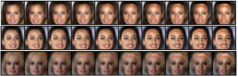
(a) Female gradually with receding hairline

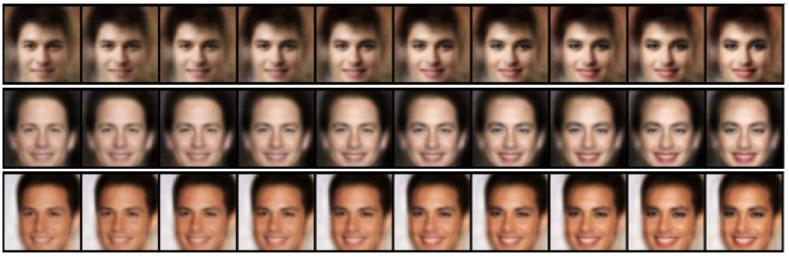
(b) Male gradually with make up

Figure 8: Sample from interventional distributions.

Learning of causal structure

CauF-VAE has the potential to learn causal structure between underlying factors, even without using a structural causal model. This is helped by the supervised loss term. Here we present the learning process of the adjacency weight matrix $A$, whose super-graph is shown in Figure 9. Figure 9(b) shows the learning process of CelebA (Attractive). If we set a threshold of 0.25, i.e., considering edges in the causal graph smaller than the threshold as non-existing, we can obtain Figure 11(e). We find that the final result differs from the true causal structure by one edge, but this also indicates that causal discovery can be further improved through future design.

Examining Causally Disentangled Representation

To verify whether our model has obtained causally disentangled representations, we consider two types of intervention operations: the "traverse" operation and the "intervention" operation introduced in Section 6.2. We present the experimental results of CauF-VAE on CelebA(Attractive) in Figure 12 and the results of baseline models on three datasets in Figure 13, 14, and 15.

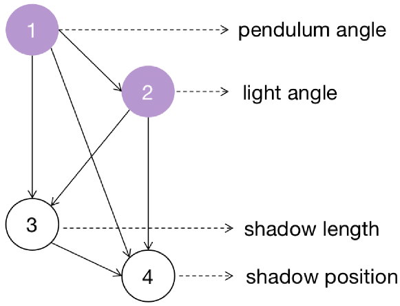
(a) Pendulum

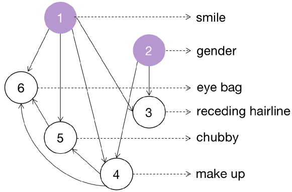
(b) CelebA(Attractive)

Figure 9: Super-graph of Pendulum and CelebA(Attractive).

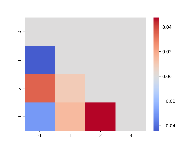
(a) Original $A$

(b) After 20 epochs

(c) After 50 epochs

(d) After 80 epochs

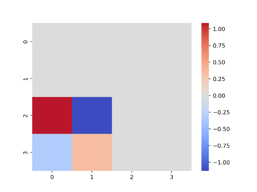
(e) Final $A$

Figure 10: The learned weighted adjacency matrix $A$ given a super-graph on Pendulum. (a)-(d) illustrate the changes in $A$ as the training progresses. (e) represents $A$ after threshold processing.

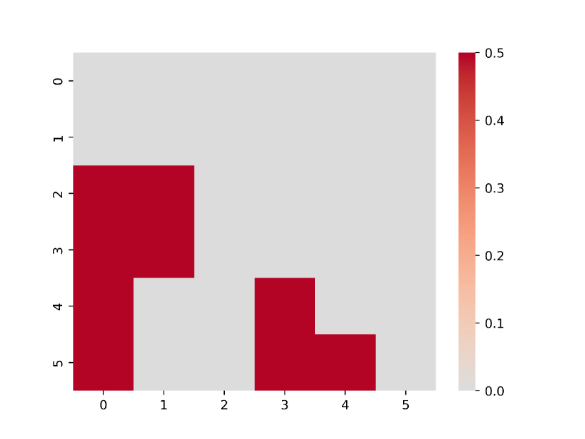
(a) Original $A$

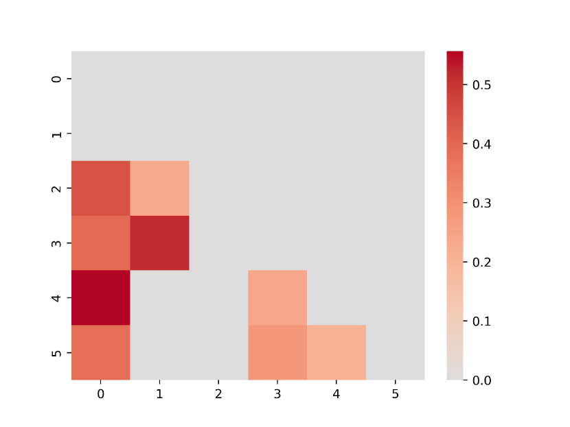
(b) After 5 epochs

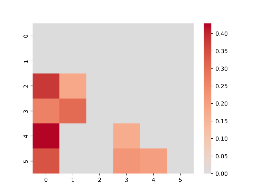
(c) After 20 epochs

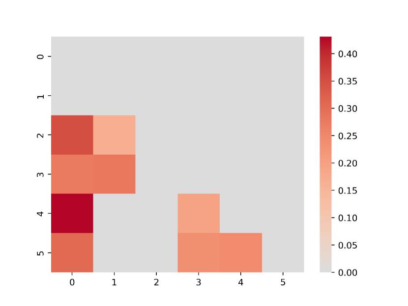
(d) After 120 epochs

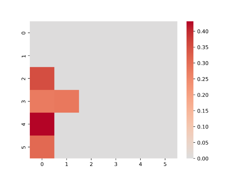
(e) Final $A$

Figure 11: The learned weighted adjacency matrix $A$ given a super-graph on CelebA(Attractive). (a)-(d) illustrate the changes in $A$ as the training progresses. (e) represents $A$ after threshold processing.

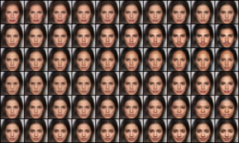
(a) Traverse of CauF-VAE on CelebA(Attractive)

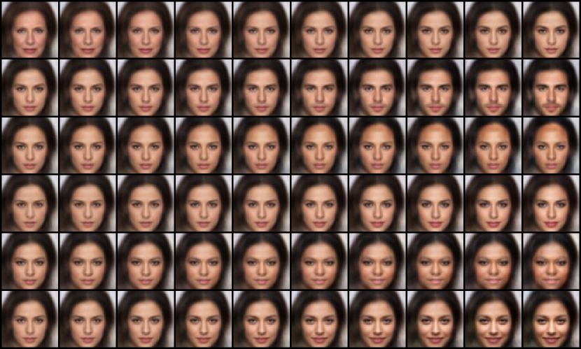
(b) Intervention of CauF-VAE on CelebA(Attractive)

Figure 12: Results of the CauF-VAE model under two types of interventions on CelebA(Atractive). Each row corresponds to one factor, in the same order as in Figure 2(b). We observe that our model achieves disentanglement, and when intervening on the causal variables, it affects the effect variables, while the opposite is not true.

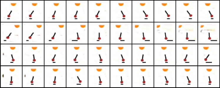
(a) DEAR

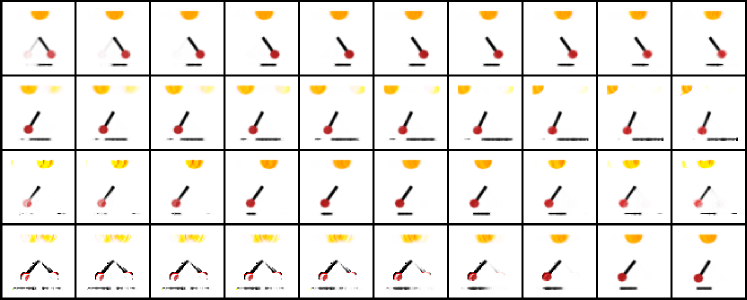
(b) $\beta$-VAE

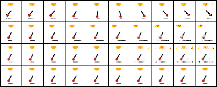
(c) $\beta$-TCVAE

(d) VAE

Figure 13: Traverse results of four baseline models on Pendulum. We observe that changing one factor may result in changes in multiple factors, or no changes in any factor, such as the shadow length in the $\beta$-TCVAE. Therefore, their representations are all entangled on Pendulum.

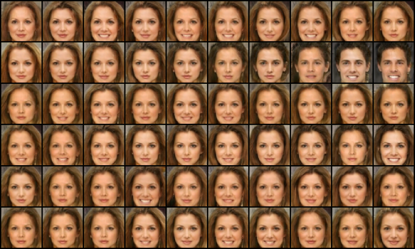
(a) DEAR

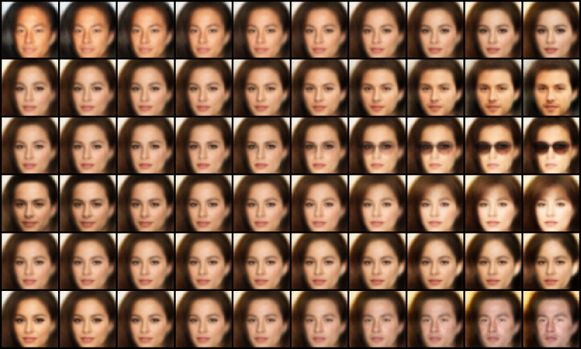
(b) $\beta$-VAE

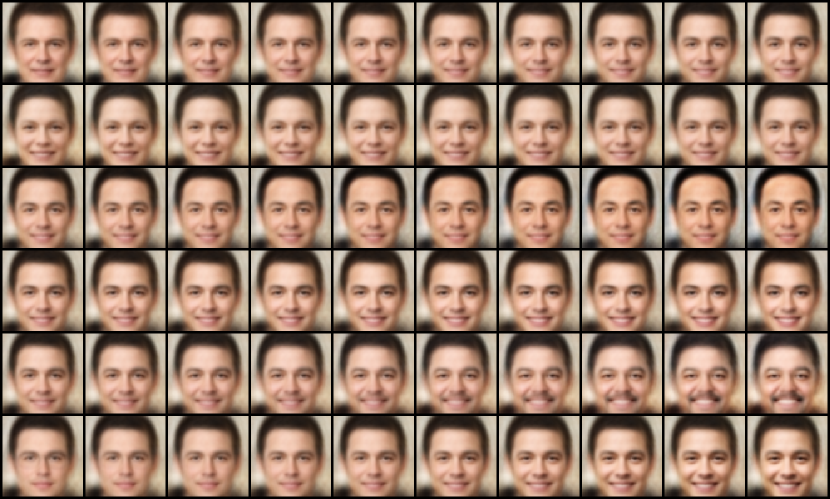
(c) $\beta$-TCVAE

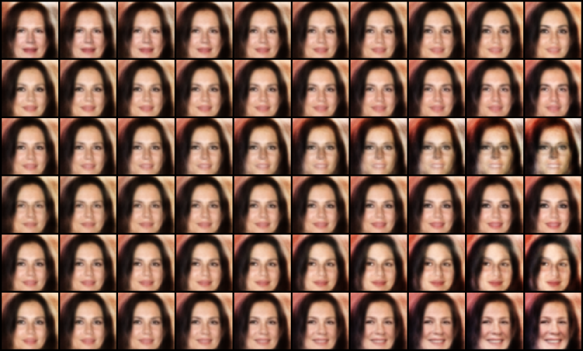
(d) VAE

Figure 14: Traverse results of four baseline models on CelebA(Attractive). We observe that the representations learned by the four models are still entangled, and some latent variables may not even capture the corresponding factor, as there is no change in the corresponding factor when traversing its value, such as the smile in the $\beta$-TCVAE.

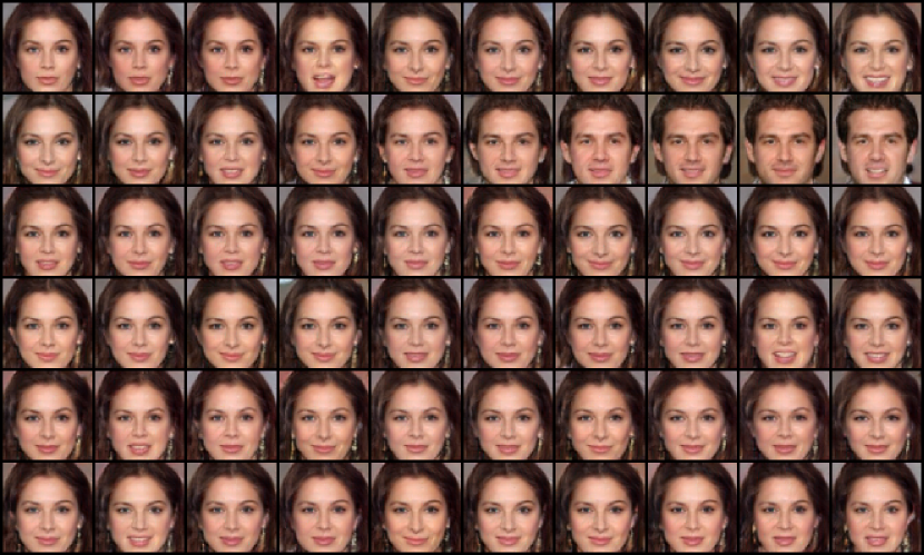
(a) DEAR

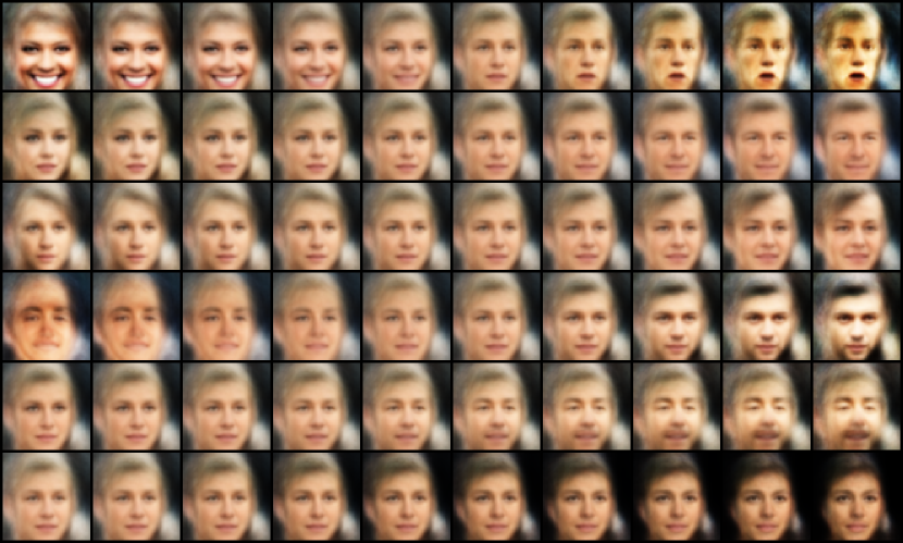
(b) $\beta$-VAE

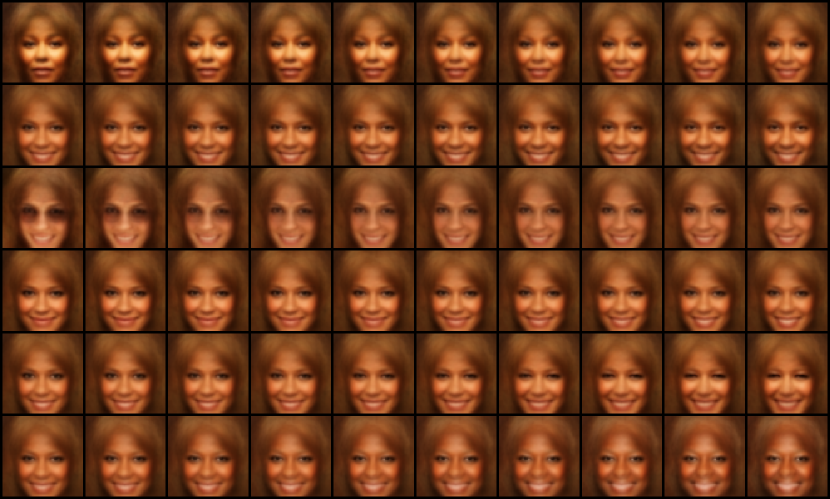
(c) $\beta$-TCVAE

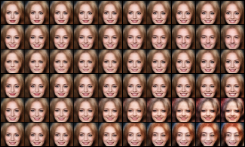
(d) VAE

Figure 15: Traverse results of four baseline models on CelebA(Smile). The representations learned by the four models are entangled. When the causal variable is changed, not only itself changes, but also the effect variable changes, such as smile and mouth open in these four figures.

References

- [1] Yoshua Bengio, Aaron Courville, and Pascal Vincent. Representation learning: A review and new perspectives. IEEE transactions on pattern analysis and machine intelligence, 35(8):1798–1828, 2013.
- [2] Francesco Locatello, Stefan Bauer, Mario Lucic, Gunnar Raetsch, Sylvain Gelly, Bernhard Schölkopf, and Olivier Bachem. Challenging common assumptions in the unsupervised learning of disentangled representations. In International conference on machine learning, pages 4114–4124. PMLR, 2019.
- [3] Diederik P Kingma and Max Welling. Auto-encoding variational bayes. arXiv preprint arXiv:1312.6114, 2013.
- [4] Irina Higgins, Loic Matthey, Arka Pal, Christopher Burgess, Xavier Glorot, Matthew Botvinick, Shakir Mohamed, and Alexander Lerchner. beta-vae: Learning basic visual concepts with a constrained variational framework. In International conference on learning representations, 2017.
- [5] Christopher P Burgess, Irina Higgins, Arka Pal, Loic Matthey, Nick Watters, Guillaume Desjardins, and Alexander Lerchner. Understanding disentangling in -vae. arXiv preprint arXiv:1804.03599, 2018.
- [6] Hyunjik Kim and Andriy Mnih. Disentangling by factorising. In International Conference on Machine Learning, pages 2649–2658. PMLR, 2018.
- [7] Ricky TQ Chen, Xuechen Li, Roger B Grosse, and David K Duvenaud. Isolating sources of disentanglement in variational autoencoders. Advances in neural information processing systems, 31, 2018.
- [8] Abhishek Kumar, Prasanna Sattigeri, and Avinash Balakrishnan. Variational inference of disentangled latent concepts from unlabeled observations. arXiv preprint arXiv:1711.00848, 2017.
- [9] Minyoung Kim, Yuting Wang, Pritish Sahu, and Vladimir Pavlovic. Relevance factor vae: Learning and identifying disentangled factors. arXiv preprint arXiv:1902.01568, 2019.
- [10] Emilien Dupont. Learning disentangled joint continuous and discrete representations. Advances in Neural Information Processing Systems, 31, 2018.
- [11] Francesco Locatello, Michael Tschannen, Stefan Bauer, Gunnar Rätsch, Bernhard Schölkopf, and Olivier Bachem. Disentangling factors of variation using few labels. arXiv preprint arXiv:1905.01258, 2019.
- [12] Xinwei Shen, Furui Liu, Hanze Dong, Qing Lian, Zhitang Chen, and Tong Zhang. Weakly supervised disentangled generative causal representation learning. Journal of Machine Learning Research, 23:1–55, 2022.
- [13] Mengyue Yang, Furui Liu, Zhitang Chen, Xinwei Shen, Jianye Hao, and Jun Wang. Causalvae: Disentangled representation learning via neural structural causal models. In Proceedings of the IEEE/CVF conference on computer vision and pattern recognition, pages 9593–9602, 2021.
- [14] Ilyes Khemakhem, Diederik Kingma, Ricardo Monti, and Aapo Hyvarinen. Variational autoencoders and nonlinear ica: A unifying framework. In International Conference on Artificial Intelligence and Statistics, pages 2207–2217. PMLR, 2020.
- [15] Francesco Locatello, Ben Poole, Gunnar Rätsch, Bernhard Schölkopf, Olivier Bachem, and Michael Tschannen. Weakly-supervised disentanglement without compromises. In International Conference on Machine Learning, pages 6348–6359. PMLR, 2020.
- [16] Frederik Träuble, Elliot Creager, Niki Kilbertus, Francesco Locatello, Andrea Dittadi, Anirudh Goyal, Bernhard Schölkopf, and Stefan Bauer. On disentangled representations learned from correlated data. In International Conference on Machine Learning, pages 10401–10412. PMLR, 2021.
- [17] Raphael Suter, Djordje Miladinovic, Bernhard Schölkopf, and Stefan Bauer. Robustly disentangled causal mechanisms: Validating deep representations for interventional robustness. In International Conference on Machine Learning, pages 6056–6065. PMLR, 2019.
- [18] Abbavaram Gowtham Reddy, Vineeth N Balasubramanian, et al. On causally disentangled representations. In Proceedings of the AAAI Conference on Artificial Intelligence, pages 8089–8097, 2022.
- [19] SeungHwan An, Kyungwoo Song, and Jong-June Jeon. Causally disentangled generative variational autoencoder. arXiv preprint arXiv:2302.11737, 2023.
- [20] Danilo Rezende and Shakir Mohamed. Variational inference with normalizing flows. In International conference on machine learning, pages 1530–1538. PMLR, 2015.
- [21] Chin-Wei Huang, David Krueger, Alexandre Lacoste, and Aaron Courville. Neural autoregressive flows. In International Conference on Machine Learning, pages 2078–2087. PMLR, 2018.
- [22] Durk P Kingma, Tim Salimans, Rafal Jozefowicz, Xi Chen, Ilya Sutskever, and Max Welling. Improved variational inference with inverse autoregressive flow. Advances in neural information processing systems, 29, 2016.
- [23] Ilyes Khemakhem, Ricardo Monti, Robert Leech, and Aapo Hyvarinen. Causal autoregressive flows. In International conference on artificial intelligence and statistics, pages 3520–3528. PMLR, 2021.
- [24] George Papamakarios, Eric Nalisnick, Danilo Jimenez Rezende, Shakir Mohamed, and Balaji Lakshminarayanan. Normalizing flows for probabilistic modeling and inference. The Journal of Machine Learning Research, 22(1):2617–2680, 2021.
- [25] Judea Pearl. Causal inference in statistics: An overview. Statistics surveys, 3:96–146, 2009.
- [26] Antoine Wehenkel and Gilles Louppe. Unconstrained monotonic neural networks. Advances in neural information processing systems, 32, 2019.
- [27] Aapo Hyvarinen and Hiroshi Morioka. Unsupervised feature extraction by time-contrastive learning and nonlinear ica. Advances in neural information processing systems, 29, 2016.
- [28] Lorenzo Pacchiardi and Ritabrata Dutta. Score matched neural exponential families for likelihood-free inference. J. Mach. Learn. Res., 23(38):1–71, 2022.
- [29] Ilyes Khemakhem, Ricardo Monti, Diederik Kingma, and Aapo Hyvarinen. Ice-beem: Identifiable conditional energy-based deep models based on nonlinear ica. Advances in Neural Information Processing Systems, 33:12768–12778, 2020.
- [30] Antoine Wehenkel and Gilles Louppe. Graphical normalizing flows. In International Conference on Artificial Intelligence and Statistics, pages 37–45. PMLR, 2021.
- [31] Ziwei Liu, Ping Luo, Xiaogang Wang, and Xiaoou Tang. Deep learning face attributes in the wild. In Proceedings of the IEEE international conference on computer vision, pages 3730–3738, 2015.
- [32] Judea Pearl. Causality. Cambridge university press, 2009.
- [33] Judea Pearl et al. Models, reasoning and inference. Cambridge, UK: CambridgeUniversityPress, 19(2), 2000.
- [34] Justin B Kinney and Gurinder S Atwal. Equitability, mutual information, and the maximal information coefficient. Proceedings of the National Academy of Sciences, 111(9):3354–3359, 2014.