Light-cone distribution amplitudes of a light baryon in large-momentum effective theory

Abstract

Momentum distributions of quarks/gluons inside a light baryon in a hard exclusive process are encoded in the light-cone distribution amplitudes (LCDAs). In this work, we point out that the leading twist LCDAs of a light baryon can be obtained through a simulation of a quasi-distribution amplitude calculable on lattice QCD within the framework of the large-momentum effective theory. We calculate the one-loop perturbative contributions to LCDA and quasi-distribution amplitudes and explicitly demonstrate the factorization of quasi-distribution amplitudes at the one-loop level. Based on the perturbative results, we derive the matching kernel in the $\overline{\rm MS}$ scheme and regularization-invariant momentum-subtraction scheme. Our result provides a first step to obtaining the LCDA from first principle lattice QCD calculations in the future.

I Introduction

Light-cone distribution amplitudes (LCDAs) of a light baryon describe the momentum distributions of a quark/gluon in a baryonic system and are a fundamental non-perturbative input in QCD factorization for an exclusive process with a large momentum transfer. An explicit example of this type is weak decays of bottom baryons which are valuable to extract the CKM matrix element in the standard model LHCb:2015eia and to probe new physics beyond the standard model LHCb:2017slr . In addition, in contrast with parton distribution functions that encode the probability density of parton momenta in hadrons, the LCDAs offer a probability amplitude description of the partonic structure of hadrons, from which one can potentially calculate various quark/gluon distributions. Thus the knowledge of LCDAs is also key to understanding the internal structure of light baryons, such as a proton.

Though many progresses have been made in obtaining the LCDAs of a nucleon in the past decades Chernyak:1984bm ; King:1986wi ; Chernyak:1987nu ; Chernyak:1987nv ; Braun:2014wpa ; RQCD:2019hps ; Stefanis:1992nw ; Bolz:1996sw ; Groote:1997yr ; Braun:2000kw ; Braun:2006hz ; QCDSF:2008qtn ; Anikin:2013aka ; Kim:2021zbz , most of the available analyses are limited to the few lowest moments of LCDAs. Due to the lack of a complete knowledge of baryon LCDAs, many phenomenological analyses adopt model paramterizations resulting in uncontrollable errors in theoretical predictions for decay branching fractions of heavy baryons Lu:2009cm ; Huang:2022lfr ; Han:2022srw . Thus, it is highly indispensable to develop a method to calculate the full shape of baryon LCDAs from the first principle of QCD.

Since LCDAs are defined as the correlation functions of lightcone operators inside a hadron, these quantities can not be directly evaluated on the lattice. In 2013, a very inspiring approach was proposed to circumvent this problem and is now formulated as the large-momentum effective theory (LaMET) Ji:2013dva ; Ji:2014gla . In LaMET, instead of directly calculating light-cone correlations, one can start from equal-time correlations in a large-momentum hadron state, which are known as quasi-distributions. The quasi-distributions share the same infrared properties with lightcone distributions and are connected to PDFs and LCDAs via a matching scheme. Under the framework of LaMET, encouraging results are recently obtained on the lattice and for recent reviews please see Refs. Cichy:2018mum ; Zhao:2018fyu ; Ji:2020ect and many references therein. Based on this approach, results on LCDAs of light mesons can be found in Refs. Zhang:2017bzy ; Zhang:2017zfe ; Zhang:2020gaj ; Hua:2020gnw ; LatticeParton:2022zqc ; Gao:2022vyh . Other methods to extract lightcone PDFs and LCDAs can also be found in Refs. Orginos:2017kos ; Radyushkin:2017cyf ; Ma:2014jla ; Ma:2017pxb .

In this work, we aim to provide an exploration of the leading twist lightcone distribution amplitude of a light baryon in LaMET. Taking the $\Lambda$ baryon as an example, we first calculate the one-loop perturbative QCD contributions to LCDAs and quasi-DAs of a light baryon. We demonstrate that these two quantities have the same infrared structure which explicitly validates the factorization at the one-loop level. We also provide an analysis based on expansion by region, which gives direct proof. Based on the one-loop results, we derive the matching kernel. To regularize remnant UV divergences, we also give the matching results in a regularization-invariant momentum-subtraction scheme. Future improvements in lattice realization will be briefly mentioned in the end.

The rest of this paper is organized as follows. In Sec. II, we present a brief review of the twist-2 LCDAs of a light baryon and the one-loop perturbative results. In Sec. III, we calculate the contributions to the quasi-DA in the modified minimal subtraction scheme. In Sec. IV, we calculate the one-loop contributions to quasi-DA with the off-shell external states with a RI/MOM subtraction. In Sec. V, we give the one-loop matching coefficients from quasi-DA to LCDA. A summary is presented in Sec. VI. Some details are provided in the appendix.

II LCDA at one loop level

In the factorization analysis of heavy-to-light baryonic transition, one is led at leading-twist to the matrix element of a three-quark operator between the vacuum and the baryon state. Taking the $\Lambda$ baryon which is made of $uds$ as an example, one can see that the LCDA is defined by the non-local light-ray operators

$$\epsilon_{ijk}\langle 0|u_{i}^{T}(t_{1}n)\Gamma d_{j}(t_{2}n)s_{k}(0)|\Lambda\rangle,$$ (1)

with $i,j,k$ being color indices. $T$ denotes the transpose in the spinor space. Under the assignment of $\bar{n}$ as the light quark flight direction, the three light quarks are separated in the $n$ direction in coordinate space. The two lightcone unit vectors are defined as $n^{\mu}=(1,0,0,-1)/\sqrt{2}$ and $\bar{n}^{\mu}=(1,0,0,1)/\sqrt{2}$. The covariant derivative is $D_{\mu}=\partial_{\mu}-igA_{\mu}$.

Two pieces of gauge links are not shown in the above formulae

$$\mathcal{W}_{ij}(0,x)=\mathcal{P}{\rm exp}\left[ig_{s}\int_{x}^{0}dtn_{\mu}A^{\mu}_{ij}(tn)\right].$$ (2)

It is worthwhile pointing out that the above form of the Wilson line is not unique, but a gauge invariant building block, e.g. for a quark field with color $i$, is

$$Q_{i}(x)=\mathcal{W}_{ii^{\prime}}(\infty,x)q_{i^{\prime}}(x),$$ (3)

and the piece from $0$ to $\infty$ is omitted in Eq. (2) since it is irrelevant of LCDA. A proof is included in Appendix A.

The collinear twist expansion makes use of the decomposition of the quark field into large and small components (see for example Braun:2003rp )

$$q=\left(\frac{n\!\!\!/\bar{n}\!\!\!/}{2}+\frac{\bar{n}\!\!\!/n\!\!\!/}{2}\right)q.$$ (4)

The large component is projected out by $\bar{n}\!\!\!/n\!\!\!/$ if quark’s flight direction is chosen $\bar{n}$, i.e. $p^{\mu}=(p^{z},0,0,p^{z})$ ($p$ is the momentum of baryon). The twist-3 LCDAs are made of three large components, and for $\Lambda$ baryon one has the explicit form

$$\Phi(x_{1},x_{2})f_{\Lambda}u_{\Lambda}(p)=\int\frac{dt_{1}p^{+}}{2\pi}\int\frac{dt_{2}p^{+}}{2\pi}e^{ix_{1}p^{+}t_{1}+ix_{2}p^{+}t_{2}}$$

$$\times\epsilon_{ijk}\langle 0|U_{i}^{T}(t_{1}n)\Gamma D_{j}(t_{2}n)S_{k}(0)|\Lambda\rangle,$$ (5)

where $\Gamma=C\gamma^{5}n\!\!\!/$, and $C=i\gamma^{2}\gamma^{0}$. $f_{\Lambda}$ is the decay constant for $\Lambda$, and $u_{\Lambda}(p)$ is the $\Lambda$ spinor. The short-distance coefficient is insensitive to the hadrons, i.e. the UV behavior of LCDAs is irrelevant to the low energy dynamics. In the calculation of LCDAs, one can replace the hadron with a partonic state with the same quantum numbers.

In the following calculation, we replace the hadron state $|\Lambda\rangle$ by three constituent quarks state, i.e. $|\Lambda\rangle\to|u_{a}(k_{1})d_{b}(k_{2})s_{c}(k_{3})\rangle$. Here $p=k_{1}+k_{2}+k_{3}$ is the momentum conservation condition. In this case, the leading twist LCDA is defined as

$$\phi(x_{1},x_{2})S$$

$$= \int\frac{dt_{1}p^{+}}{2\pi}\int\frac{dt_{2}p^{+}}{2\pi}e^{ix_{1}p^{+}t_{1}+ix_{1}p^{+}t_{2}}\frac{\epsilon_{ijk}\epsilon_{abc}}{6}$$

$$\times \langle 0|U_{i}^{T}(t_{1}n)\Gamma D_{j}(t_{2}n)S_{k}(0)|u_{a}(k_{1})d_{b}(k_{2})s_{c}(k_{3})\rangle,$$

where $p^{+}=n\cdot p$, $x_{i,0}={k_{i}^{+}}/{p^{+}}$, $\sum_{i=1}^{3}x_{i}=1$, $\sum_{i=1}^{3}x_{i,0}=1$, and all longitudinal momentum fractions carried by baryons satisfy $0<x_{i,0}<1$. The normalization factor $S$ can be constructed in terms of the partonic local operator matrix element:

$$S = \frac{\epsilon_{ijk}\epsilon_{abc}}{6}\langle 0|(U_{i})^{T}(0)\Gamma D_{j}(0)S_{k}(0)|u_{a}(k_{1})d_{b}(k_{2})s_{c}(k_{3})\rangle.$$

At tree level, we have

$$S^{(0)} = -\frac{\epsilon_{abc}\epsilon_{abc}}{6}\Big{[}{u^{s_{1}}(k_{1})}\Big{]}^{T}\Gamma u^{s_{2}}(k_{2})u(k_{3})$$ (8)

$$= 2p^{+}u(k_{3}),$$

where $\Big{[}{u^{s_{1}}(k_{1})}\Big{]}^{T}\Gamma u^{s_{2}}(k_{2})=\frac{1}{2}{\rm{tr}}\big{[}\not{p}C\gamma^{5}\Gamma\big{]}$ is employed, and the superscript index ‘$(0)$’ refer to tree-level result. Here, the quark state is chosen to have the same $J^{PC}$ with the $\Lambda$, and the spin average and color average are assumed in this calculation. In Appendix B, we provide a detailed explanation of Eq. (8), and the corresponding trace formalism to derive this convention.

After a bit of algebra, we obtain the result of LCDA at the tree level

$$\phi^{(0)}(x_{1},x_{2},\mu)S^{(0)} = \int\frac{dt_{1}p^{+}}{2\pi}\int\frac{dt_{2}p^{+}}{2\pi}e^{ip^{+}(x_{1}t_{1}+x_{2}t_{2})}$$ (9)

$$\times\Big{[}{u^{s_{1}}(k_{1})}\Big{]}^{T}\Gamma u^{s_{2}}(k_{2})u(k_{s})$$

$$\times e^{-ik_{1}^{+}t_{1}}e^{-ik_{2}^{+}t_{2}}$$

$$= \delta(x_{1}-x_{1,0})\delta(x_{2}-x_{2,0})S^{(0)},$$

i.e.

$$\phi^{(0)}(x_{1},x_{2},\mu) = \delta(x_{1}-x_{1,0})\delta(x_{2}-x_{2,0}).$$ (10)

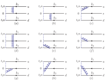
Figure 1: One-loop corrections to LCDAs of a light baryon $\Lambda$.

At the one-loop order, two gluons are radiated from (1) light quarks by the QCD interactions and (2) two pieces of gauge-link. These five objects give $C_{5}^{2}=10$ terms with five self-energy corrections in total. The diagram from two gauge links is zero since $n^{2}=0$ and the rest is displayed in Fig. 1 (quark self-energy corrections are not shown). We choose the dimensional regularization $D=4-2\epsilon$ to regularize the UV and IR divergences.

The real diagram shown in Fig. 1(a) can be obtained:

$$\mathcal{M}^{a} = ig^{2}\frac{-C_{F}}{2}(p^{+})^{2}\Big{(}\frac{\mu^{2}}{e^{\ln(4\pi)-\gamma_{E}}}\Big{)}^{\epsilon}\int\frac{d^{D}q}{(2\pi)^{D}}\frac{1}{q^{2}+i\epsilon}$$

$$\times\frac{1}{(k_{3}-q)^{2}+i\epsilon}\frac{\delta(x_{1}p^{+}-q^{+}-k_{1}^{+})\delta(x_{2}p^{+}-k_{2}^{+})}{(q+k_{1})^{2}+i\epsilon}$$

$$\times\big{[}{u^{s_{1}}(k_{1})}\big{]}^{T}\gamma^{\mu}(\not{q}+{\not{k_{1}}})\Gamma u^{s_{2}}(k_{2})({\not{k_{3}}}-{\not{q}})\gamma_{\mu}u(k_{3})$$

$$= ig^{2}\frac{-C_{F}}{2}(p^{+})^{2}\Big{(}\frac{\mu^{2}}{e^{\ln(4\pi)-\gamma_{E}}}\Big{)}^{\epsilon}\int\frac{d^{D}q}{(2\pi)^{D}}\frac{1}{q^{2}+i\epsilon}$$

$$\times\frac{\delta(x_{1}p^{+}-q^{+}-k_{1}^{+})\delta(x_{2}p^{+}-k_{2}^{+})}{(q+k_{1})^{2}+i\epsilon}\frac{1}{(k_{3}-q)^{2}+i\epsilon}\$$

$$\times\frac{1}{2}(-1){\rm tr}\left(\not{p}\gamma^{5}\gamma^{\mu}(\not{q}+\not{k_{1}})\gamma^{5}\not{n}\right)({\not{k_{3}}}-{\not{q}})\gamma_{\mu}u(k_{3}),$$

where $\mu$ is the renormalization scale in the $\overline{\rm{MS}}$ scheme, and $\mathcal{M}$ denotes $\phi(x_{1},x_{2},\mu)S$ in short. The color factor is $-\frac{C_{F}}{2}$ which comes from color Fierz transformation:

$$\frac{\epsilon_{ijk}\epsilon_{abc}}{6}T^{A}_{ia}T^{A}_{kc}\delta_{jb}=\frac{\epsilon_{ijk}\epsilon_{abc}}{6}\frac{\delta_{jb}}{2}\left(\delta_{ic}\delta_{ak}-\frac{1}{N_{c}}\delta_{ia}\delta_{kc}\right).$$

The spinor part in the last line of Eq. (II) can be projected out by taking the projection technique, i.e.

$$\frac{1}{2}\times(-1){\rm tr}\left(\not{p}\gamma^{5}\gamma^{\mu}(\not{q}+\not{k_{1}})\gamma^{5}\not{n}\right)({\not{k_{3}}}-{\not{q}})\gamma_{\mu}u(k_{3})$$ (13)

$$= \big{(}-q_{\perp}^{2}-q^{-}q_{\perp}\not{n}\not{n}_{\perp}\big{)}S^{(0)},$$

and the integration of the second term is zero because the integrated function for $q_{\perp}$ is odd. Finally, the amplitude of Fig. 1(a) can be simplified to

$$\mathcal{M}^{a}=\frac{\alpha_{s}C_{F}}{8\pi}\delta(x_{2}-x_{2,0})\theta(x_{1})\theta(x_{3})\theta(1-x_{1})\theta(1-x_{3})$$

$$\times\Bigg{[}\frac{x_{3}\theta(x_{1}-x_{1,0})}{(1-x_{2})x_{3,0}}+\frac{x_{1}\theta(x_{1,0}-x_{1})}{(1-x_{2})x_{1,0}}\Bigg{]}\Big{(}\frac{1}{\epsilon_{\rm UV}}-\frac{1}{\epsilon_{\rm IR}}\Big{)}S^{(0)},$$

where we use $\alpha_{s}=\alpha_{s}(\mu)$ in short.

In a similar way, the real diagram Fig. 1(d) can be obtained as follows:

$$\mathcal{M}^{d} = ig^{2}\frac{-C_{F}}{2}(p^{+})^{2}\Big{(}\frac{\mu^{2}}{e^{\ln(4\pi)-\gamma_{E}}}\Big{)}^{\epsilon}\int\frac{d^{D}q}{(2\pi)^{D}}\frac{1}{q^{2}+i\epsilon}$$

$$\times\frac{1}{(k_{2}-q)^{2}+i\epsilon}\frac{\delta(\omega_{1}-k_{1}^{+}-q^{+})\delta(\omega_{2}-k_{2}^{+}+q^{+})}{(k_{1}+q)^{2}+i\epsilon}$$

$$\times\big{[}{u^{s_{1}}(k_{1})}\big{]}^{T}\gamma^{\mu}(\not{k_{1}}+\not{q})\Gamma(\not{k_{2}}-\not{q})\gamma_{\mu}u^{s_{2}}(k_{2})u(k_{3})$$

$$= \frac{\alpha_{s}C_{F}}{4\pi}\delta(x_{3}-x_{3,0})\theta(x_{1})\theta(x_{2})\theta(1-x_{1})\theta(1-x_{2})$$

$$\times\Big{[}\frac{x_{2}\theta(x_{1}-x_{1,0})}{(x_{1}+x_{2})x_{2,0}}+\frac{x_{1}\theta(x_{2}-x_{2,0})}{(x_{1}+x_{2})x_{1,0}}\Big{]}(\frac{1}{\epsilon_{\rm UV}}-\frac{1}{\epsilon_{\rm IR}})S^{(0)}.$$

This result is symmetric under the exchange $x_{1}\leftrightarrow x_{2}$ and $x_{1,0}\leftrightarrow x_{2,0}$. At the same time, we should also note that in addition to the color factor $-\frac{C_{F}}{2}$, the normalization factor $S^{(0)}$, and the fraction $\frac{\delta(x_{3}-x_{3,0})}{x_{1}+x_{2}}$, which is the same as the contribution of the pseudo scalar $\pi$ meson distribution amplitude to the external leg exchange gluon diagram.

The result of Fig. 1(b) can be obtained from the result of Fig. 1(a) with $x_{2}\leftrightarrow x_{1}$ and $x_{2,0}\leftrightarrow x_{1,0}$. Therefore, we can write the result of Fig. 1(b) as follows

$$\mathcal{M}^{b}=\frac{\alpha_{s}C_{F}}{8\pi}\delta(x_{1}-x_{1,0})\theta(x_{2})\theta(x_{3})\theta(1-x_{2})\theta(1-x_{3})$$

$$\times\Bigg{[}\frac{x_{3}\theta(x_{2}-x_{2,0})}{(1-x_{1})x_{3,0}}+\frac{x_{2}\theta(x_{2,0}-x_{2})}{(1-x_{1})x_{2,0}}\Bigg{]}\Big{(}\frac{1}{\epsilon_{\rm UV}}-\frac{1}{\epsilon_{\rm IR}}\Big{)}S^{(0)}.$$

For the diagram Fig. 1(c), we have

$$\mathcal{M}^{c} =-ig^{2}C_{F}p^{+}\delta(x_{2}-x_{2,0})\Big{(}\frac{\mu^{2}}{e^{\ln(4\pi)-\gamma_{E}}}\Big{)}^{\epsilon}\int\frac{d^{D}q}{(2\pi)^{D}}\frac{1}{q^{+}}$$ (17)

$$\times\frac{1}{q^{2}+i\epsilon}\frac{\delta\big{(}(x_{1}-x_{1,0})p^{+}-q^{+}\big{)}-\delta\big{(}(x_{1}-x_{1,0})p^{+}\big{)}}{(q+k_{1})^{2}+i\epsilon}$$

$$\times(u^{s_{1}}(k_{1}))^{T}\gamma^{\mu}(\not{q}+\not{k_{1}})\Gamma u^{s_{2}}(k_{2})n_{\mu}u(k_{3}).$$

We should note that the color factor $C_{F}$ in diagram Fig. 1(c) and its symmetric diagram Fig. 1(e) are different from the other graphs. That is because Fig. 1(c) and Fig. 1(e) have no change the color structure. After simplifying Eq. (17), we have

$$\mathcal{M}^{c} = -\frac{\alpha_{s}C_{F}}{2\pi}\Bigg{[}\delta(x_{2}-x_{2,0})\theta(x_{1})\theta(x_{3})\theta(1-x_{1})\theta(1-x_{3})$$ (18)

$$\times\frac{\theta(x_{1,0}-x_{1})}{(x_{1}-x_{1,0})}\frac{x_{1}}{x_{1,0}}\Bigg{]}_{\oplus}\big{(}\frac{1}{\epsilon_{\rm UV}}-\frac{1}{\epsilon_{\rm IR}}\big{)}S^{(0)},$$

where the $\oplus$ denote

$$\left[g\left(x_{1},x_{2},x_{1,0},x_{2,0}\right)\right]_{\oplus} = g\left(x_{1},x_{2},x_{1,0},x_{2,0}\right)$$

$$-\delta\left(x_{1}-x_{1,0}\right)\delta\left(x_{2}-x_{2,0}\right)$$

$$\times\int dy_{1}dy_{2}g\left(y_{1},y_{2},x_{1,0},x_{2,0}\right).$$

The result of Fig. 1(e) can be also obtained from the result of Fig. 1(c) with $x_{2}\leftrightarrow x_{1}$ and $x_{2,0}\leftrightarrow x_{1,0}$,

$$\mathcal{M}^{e} = -\frac{\alpha_{s}C_{F}}{2\pi}\Bigg{[}\delta(x_{1}-x_{1,0})\theta(x_{2})\theta(x_{3})\theta(1-x_{2})\theta(1-x_{3})$$ (20)

$$\times\frac{\theta(x_{2,0}-x_{2})}{(x_{2}-x_{2,0})}\frac{x_{2}}{x_{2,0}}\Bigg{]}_{\oplus}\big{(}\frac{1}{\epsilon_{\rm UV}}-\frac{1}{\epsilon_{\rm IR}}\big{)}S^{(0)}.$$

We should also notice that the results for Fig. 1(c) and Fig. 1(e) are the similar to the result of the $\pi$ meson distribution amplitude to the diagram which connected the quark and the Wilson line.

For completeness of the calculation, we present the results of the other two diagrams Fig. 1(f)(h).

$$\mathcal{M}^{f} = -ig^{2}\frac{-C_{F}}{2}p^{+}\delta(x_{2}-x_{2,0})\Big{(}\frac{\mu^{2}}{e^{\ln(4\pi)-\gamma_{E}}}\Big{)}^{\epsilon}\int\frac{d^{D}q}{(2\pi)^{D}}$$ (21)

$$\frac{\delta(x_{1}p^{+}-k_{1}^{+}-q^{+})-\delta(x_{1}p^{+}-k_{1}^{+})}{q^{+}(q^{2}+i\epsilon)}\frac{1}{(k_{3}-q)^{2}+i\epsilon}$$

$$\times\big{[}{u^{s_{1}}(k_{1})}\big{]}^{T}\Gamma u^{s_{2}}(k_{2})n^{\mu}(\not{k_{3}}-\not{q})\gamma_{\mu}u(k_{3}),$$

$$= \frac{\alpha_{s}C_{F}}{4\pi}\Bigg{[}\delta(x_{2}-x_{2,0})\theta(x_{1})\theta(1-x_{1})\theta(x_{3})\theta(1-x_{3})$$

$$\times\frac{\theta(x_{1}-x_{1,0})x_{3}}{(x_{1}-x_{1,0})x_{3,0}}\Bigg{]}_{\oplus}\big{(}\frac{1}{\epsilon_{\rm UV}}-\frac{1}{\epsilon_{\rm IR}}\big{)}S^{(0)},$$

and

$$\mathcal{M}^{h} = -ig^{2}\frac{-C_{F}}{2}(p^{+})^{2}\Big{(}\frac{\mu^{2}}{e^{\ln(4\pi)-\gamma_{E}}}\Big{)}^{\epsilon}\int\frac{d^{D}q}{(2\pi)^{D}}$$ (22)

$$\times\frac{\delta(x_{2}p^{+}-k_{2}^{+})-\delta(x_{2}p^{+}+q^{+}-k_{2}^{+})}{q^{+}}$$

$$\times\frac{\delta(x_{1}p^{+}-q^{+}-k_{1}^{+})}{\big{[}q^{2}+i\epsilon\big{]}\big{[}(q+k_{1})^{2}+i\epsilon\big{]}}$$

$$\times\big{[}u^{s_{1}}(k_{1})\big{]}^{T}\gamma^{\mu}(\not{q}+\not{k_{1}})\Gamma n_{\mu}(u^{s_{2}}(k_{2}))u(k_{3}),$$

$$= \frac{\alpha_{s}C_{F}}{4\pi}\Big{[}\delta(x_{2}-x_{2,0})-\delta(x_{3}-x_{3,0})\Big{]}\theta(x_{1})\theta(1-x_{1})$$

$$\times\frac{x_{1}\theta(x_{1,0}-x_{1})}{(x_{1}-x_{1,0})x_{1,0}}\Big{(}\frac{1}{\epsilon_{\rm UV}}-\frac{1}{\epsilon_{\rm IR}}\Big{)}S^{(0)}.$$

Therefore,

$$\mathcal{M}^{g} = \frac{\alpha_{s}C_{F}}{4\pi}\Bigg{[}\delta(x_{1}-x_{1,0})\theta(x_{2})\theta(1-x_{2})\theta(x_{3})\theta(1-x_{3})$$ (23)

$$\times\frac{\theta(x_{2}-x_{2,0})x_{3}}{(x_{2}-x_{2,0})x_{3,0}}\Bigg{]}_{\oplus}\big{(}\frac{1}{\epsilon_{\rm UV}}-\frac{1}{\epsilon_{\rm IR}}\big{)}S^{(0)},$$

and

$$\mathcal{M}^{i} = \frac{\alpha_{s}C_{F}}{4\pi}\Big{[}\delta(x_{1}-x_{1,0})-\delta(x_{3}-x_{3,0})\Big{]}\theta(x_{2})\theta(1-x_{2})$$ (24)

$$\times\frac{x_{2}\theta(x_{2,0}-x_{2})}{(x_{2}-x_{2,0})x_{2,0}}\Big{(}\frac{1}{\epsilon_{\rm UV}}-\frac{1}{\epsilon_{\rm IR}}\Big{)}S^{(0)}.$$

Combining the above results with Eq. (76), we have the complete result for the one-loop normalized and $\overline{\rm MS}$ renormalized LCDA as

$$\phi(x_{1},x_{2},\mu) = \delta(x_{1}-x_{1,0})\delta(x_{2}-x_{2,0})$$ (25)

$$-\frac{\alpha_{s}C_{F}}{8\pi}\frac{1}{\epsilon_{\rm IR}}f(x_{1},x_{2},x_{1,0},x_{2,0}),$$

with

$$f(x_{1},x_{2},x_{1,0},x_{2,0})=$$

$$\Bigg{\{}\frac{\delta(x_{1}-x_{1,0})\theta(x_{1})\theta(\bar{x}_{1})\theta(x_{2})\theta(\bar{x}_{2})}{\bar{x}_{1}\left(x_{2}-x_{2,0}\right)}$$

$$\times\Big{[}\frac{x_{3}\left(x_{2}-x_{2,0}+2\bar{x}_{1}\right)}{x_{3,0}}\theta\left(x_{2}-x_{2,0}\right)$$

$$+\frac{x_{2}\left(x_{2}-x_{2,0}-2\bar{x}_{1}\right)}{x_{2,0}}\theta\left(x_{2,0}-x_{2}\right)\Big{]}$$

$$+\frac{\delta(x_{3}-x_{3,0})2x_{1}\theta(x_{1})\theta(\bar{x}_{1})\theta(x_{2})\theta(\bar{x}_{2})}{x_{1,0}}$$

$$\times\Big{[}\frac{\theta\left(x_{2}-x_{2,0}\right)}{x_{1}+x_{2}}-\frac{\theta\left(x_{1,0}-x_{1}\right)}{x_{1}-x_{1,0}}\Big{]}$$

$$+\{x_{1}\leftrightarrow x_{2},x_{1,0}\leftrightarrow x_{2,0}\}\Bigg{\}}_{\oplus},$$ (26)

where $\bar{x}=1-x$.

The renormalized LCDA can be obtained by removing the UV divergence due to the renormalization of the composite operator of LCDA. The dependence of the renormalized LCDA $\Phi(x_{1},x_{2},\mu)$ on $\ln\mu$ can be obtained from the evolution equation

$$\frac{d\Phi(x_{1},x_{2},\mu)}{d\ln\mu}=\frac{\alpha_{s}C_{F}}{4\pi}\int dy_{1}\int dy_{2}V\Phi(y_{1},y_{2},\mu).$$ (27)

At the one-loop, the evolution kernel $V$ is

$$V=f(x_{1},x_{2},y_{1},y_{2}).$$ (28)

We should also note that the form of Eq. (27) is similar to the Efremov-Radyushkin-Brodsky-Lepage (ERBL) evolution equation for mesons Lepage:1979zb ; Efremov:1979qk .

III Quasi-DA at one loop level

In this section, we will introduce an equal-time operator matrix element which is often named as quasi-distribution amplitudes Ji:2013dva . The quasi-DA for the $\Lambda$ is defined as

$$\tilde{\Phi}(x_{1},x_{2},\mu)\tilde{f}_{\Lambda}u_{\Lambda}(p) =\int\frac{dt_{1}p^{z}}{2\pi}\int\frac{dt_{2}p^{z}}{2\pi}e^{ix_{1}p^{z}t_{1}+ix_{1}p^{z}t_{2}}$$

$$\times\epsilon_{ijk}\langle 0|U_{i}^{T}(t_{1}n_{z})\tilde{\Gamma}D_{j}(t_{2}n_{z})S_{k}(0)|\Lambda\rangle,$$

where $\tilde{f}_{\Lambda}$ is the quasi decay constant for $\Lambda$.

In a similar way, the corresponding partonic operator matrix element is

$$\tilde{\phi}(x_{1},x_{2},\mu)\tilde{S}$$

$$= \int\frac{dt_{1}p^{z}}{2\pi}\int\frac{dt_{2}p^{z}}{2\pi}e^{ix_{1}p^{z}t_{1}+ix_{1}p^{z}t_{2}}\frac{\epsilon_{ijk}\epsilon_{abc}}{6}\times$$

$$\langle 0|(U_{i})^{T}(t_{1}n_{z})\tilde{\Gamma}D_{j}(t_{2}n_{z})S_{k}(0)|u_{a}(k_{1})d_{b}(k_{2})s_{c}(k_{3})\rangle.$$

The $\tilde{\Gamma}$ is the Dirac matrix for the quasi-DA and two popular choices are $\tilde{\Gamma}=C\gamma^{5}\not{n}_{\lambda}$ ($\lambda=t$ or $z$) for quasi-DA. The two choices will give the same results at leading twist and a brief explanation is given in Appendix C. Here $n_{t}^{\mu}=(1,0,0,0)$ and $n_{z}^{\mu}=(0,0,0,-1)$. The corresponding normalization factor $\tilde{S}$ is

$$\tilde{S} = \frac{\epsilon_{ijk}\epsilon_{abc}}{6}\langle 0|(U_{i})^{T}(0)\tilde{\Gamma}D_{j}(0)S_{k}(0)|u_{a}(k_{1})d_{b}(k_{2})s_{c}(k_{3})\rangle.$$

At the tree level, we have the matrix element

$$\tilde{S}^{(0)} = -\frac{\epsilon_{abc}\epsilon_{abc}}{6}\Big{[}{u^{s_{1}}(k_{1})}\Big{]}^{T}\tilde{\Gamma}u^{s_{2}}(k_{2})u(k_{3})$$ (32)

$$= 2p^{z}u(k_{3}),$$

where $\Big{[}{u^{s_{1}}(k_{1})}\Big{]}^{T}\tilde{\Gamma}u^{s_{2}}(k_{2})=\frac{1}{2}{\rm{tr}}\big{[}\not{p}C\gamma^{5}\tilde{\Gamma}\big{]}$ is employed. The tree-level result for quasi-DA is

$$\tilde{\phi}^{(0)}(x_{1},x_{2},\mu)\tilde{S}^{(0)} = {p^{z}}^{2}\int\frac{dt_{1}}{2\pi}\int\frac{dt_{2}}{2\pi}e^{ix_{1}t_{1}p^{z}+ix_{2}t_{2}p^{z}}$$ (33)

$$\times\Big{[}{u^{s_{1}}(k_{1})}\Big{]}^{T}\tilde{\Gamma}u^{s_{2}}(k_{2})u(k_{3})$$

$$\times e^{-ix_{1,0}p^{z}t_{1}}e^{-ix_{2,0}p^{z}t_{2}}$$

$$= \delta(x_{1}-x_{1,0})\delta(x_{2}-x_{2,0})\tilde{S}^{(0)}.$$

Therefore, the normalized quasi-DA at the tree level is

$$\tilde{\phi}^{(0)}(x_{1},x_{2},\mu)=\delta(x_{1}-x_{1,0})\delta(x_{2}-x_{2,0}).$$ (34)

We can find that the normalized LCDA at the tree-level gives the same result as the quasi-DA. The one-loop diagrams of quasi-DA for baryon $\Lambda$ are similar to that of the LCDA which are shown in Fig. 1, except the $n$ direction is changed to $n_{z}$. The real diagram for quasi-DA shown in Fig. 1(a) can be obtained as follows:

$$\tilde{\mathcal{M}}^{a} = ig^{2}\frac{-C_{F}}{2}{p^{z}}^{2}\Big{(}\frac{\mu^{2}}{e^{\ln(4\pi)-\gamma_{E}}}\Big{)}^{\epsilon}\int\frac{d^{D}q}{(2\pi)^{D}}\frac{1}{q^{2}+i\epsilon}$$

$$\times\frac{1}{(k_{3}-q)^{2}+i\epsilon}\frac{\delta(x_{1}p^{z}-q^{z}-{k_{1}}^{z})\delta(x_{2}p^{z}-{k_{2}}^{z})}{(q+k_{1})^{2}+i\epsilon}$$

$$\times\big{[}{u^{s_{1}}(k_{1})}\big{]}^{T}\gamma^{\mu}(\not{q}+{\not{k_{1}}})\tilde{\Gamma}u^{s_{2}}(k_{2})({\not{k_{3}}}-{\not{q}})\gamma_{\mu}u(k_{3}),$$

$$= ig^{2}\frac{-C_{F}}{2}{p^{z}}^{2}\Big{(}\frac{\mu^{2}}{e^{\ln(4\pi)-\gamma_{E}}}\Big{)}^{\epsilon}\int\frac{d^{D}q}{(2\pi)^{D}}\frac{1}{q^{2}+i\epsilon}$$

$$\times\frac{1}{(k_{3}-q)^{2}+i\epsilon}\frac{\delta(x_{1}p^{z}-q^{z}-{k_{1}}^{z})\delta(x_{2}p^{z}-{k_{2}}^{z})}{(q+k_{1})^{2}+i\epsilon}$$

$$\times(-\frac{1}{2}){\rm tr}\left(\not{p}\gamma^{5}\gamma^{\mu}(\not{q}+\not{k_{1}})\gamma^{5}\not{n}_{\lambda}\right)({\not{k_{3}}}-{\not{q}})\gamma_{\mu}u(k_{3}),$$

where $\tilde{\mathcal{M}}$ denotes $\tilde{\phi}(x_{1},x_{2},\mu)\tilde{S}$ in short. The last line in the above equation reads

$$-\frac{1}{2}{\rm tr}\left(\not{p}\gamma^{5}\gamma^{\mu}(\not{q}+\not{k_{1}})\gamma^{5}\gamma^{\lambda}\right)({\not{k_{3}}}-{\not{q}})\gamma_{\mu}u(k_{3})$$ (36)

$$= \big{[}q^{2}-(p\cdot q)\frac{q^{t}+q^{z}}{p^{z}}-q_{\perp}\not{n}_{\perp}\not{n}_{z}\big{]}\tilde{S}^{(0)},$$

and the third term gives zero contribution because the integrand as in Eq. (III) is odd in $q_{\perp}$. This result indicates the equivalence of the two Lorentz structures $\tilde{\Gamma}$.

Finally, the quasi-DA in Fig. 1(a) can be simplified as

$$\tilde{\mathcal{M}}^{a}=\frac{\alpha_{s}C_{F}}{8\pi}\tilde{S}^{(0)}\delta(x_{2}-x_{2,0})$$

$$\times\left\{\begin{aligned} &\Big{[}\frac{x_{1}\ln\frac{-x_{1}}{x_{3}}}{(1-x_{2,0})x_{3,0}}-\frac{x_{1}\ln\frac{-x_{1}}{x_{1,0}-x_{1}}}{x_{1,0}x_{3,0}}-\frac{\ln\frac{x_{1,0}-x_{1}}{x_{3}}}{x_{3,0}}\Big{]},~{}x_{1}<0\\ &\Big{[}\frac{x_{1}\left(\ln\frac{(x_{1,0}-x_{1})x_{1}}{\mu^{2}/({2p^{z}})^{2}}-1\right)}{x_{1,0}x_{3,0}}-\frac{x_{1}\left(\ln\frac{x_{1}x_{3}}{\mu^{2}/({2p^{z}})^{2}}-1\right)}{\left(1-x_{2,0}\right)x_{3,0}}-\frac{\ln\frac{x_{1,0}-x_{1}}{x_{3}}}{x_{3,0}}-\frac{x_{1}}{x_{1,0}\left(1-x_{2,0}\right)}\frac{1}{\epsilon_{\rm IR}}\Big{]},~{}0<x_{1}<x_{1,0}\\ &\Big{[}\frac{x_{1}\ln\frac{x_{1}}{x_{1}-x_{1,0}}}{x_{1,0}x_{3,0}}-\frac{x_{1}\left(\ln\frac{x_{1}x_{3}}{\mu^{2}/({2p^{z}})^{2}}-1\right)}{\left(1-x_{2,0}\right)x_{3,0}}+\frac{\ln\frac{(x_{1}-x_{1,0})x_{3}}{\mu^{2}/({2p^{z}})^{2}}-1}{x_{3,0}}-\frac{x_{3}}{x_{3,0}\left(1-x_{2,0}\right)}\frac{1}{\epsilon_{\rm IR}}\Big{]},~{}x_{1,0}<x_{1}<1-x_{2}\\ &\Big{[}\frac{x_{1}\ln\frac{x_{1}}{x_{1}-x_{1,0}}}{x_{1,0}x_{3,0}}+\frac{x_{1}\ln\frac{-x_{3}}{x_{1}}}{\left(1-x_{2,0}\right)x_{3,0}}+\frac{\ln\frac{x_{1}-x_{1,0}}{-x_{3}}}{x_{3,0}}\Big{]}.~{}x_{1}>1-x_{2}\\ \end{aligned}\right.$$ (37)

For the remaining diagrams, rather than enumerating the calculations in detail, we directly give their results

$$\tilde{\mathcal{M}}^{b}=\tilde{\mathcal{M}}^{a}|_{x_{2}\leftrightarrow x_{1},x_{2,0}\leftrightarrow x_{1,0}},$$ (38)

$$\tilde{\mathcal{M}}^{d}=\frac{\alpha_{s}C_{F}}{4\pi}\tilde{S}^{(0)}\delta(x_{1}+x_{2}-x_{1,0}-x_{2,0})$$

$$\times\left\{\begin{aligned} &\Big{[}\frac{x_{1}}{x_{1,0}(x_{1,0}+x_{2,0})}\ln\frac{x_{2}}{-x_{1}}+\frac{x_{2,0}-x_{2}}{x_{1,0}x_{2,0}}\ln\frac{x_{2}-x_{2,0}}{x_{2}}\Big{]},~{}x_{1}<0\\ &\Big{\{}\frac{x_{1}\Big{[}\ln\left(\frac{x_{1}x_{2}}{\mu^{2}/({2p^{z}})^{2}}\right)+1\Big{]}}{x_{1,0}\left(x_{1,0}+x_{2,0}\right)}+\frac{\left(x_{2}-x_{2,0}\right)\ln\frac{x_{2}}{x_{2}-x_{2,0}}}{x_{1,0}x_{2,0}}-\frac{x_{1}}{x_{1,0}\left(x_{1,0}+x_{2,0}\right)}\frac{1}{\epsilon_{\rm IR}}\Big{\}},~{}0<x_{1}<x_{1,0}\\ &\Big{\{}\frac{x_{1}\Big{[}\ln\left(\frac{x_{1}x_{2}}{\mu^{2}/({2p^{z}})^{2}}\right)+1\Big{]}}{x_{1,0}\left(x_{1,0}+x_{2,0}\right)}+\frac{\left(x_{2}-x_{2,0}\right)\Big{[}\ln\frac{x_{2}(x_{2,0}-x_{2})}{\mu^{2}/({2p^{z}})^{2}}+1\Big{]}}{x_{1,0}x_{2,0}}-\frac{x_{2}}{x_{2,0}\left(x_{1,0}+x_{2,0}\right)}\frac{1}{\epsilon_{\rm IR}}\Big{\}},x_{1,0}<x_{1}<x_{1}+x_{2}\\ &\Big{[}\frac{x_{1}}{x_{1,0}(x_{1,0}+x_{2,0})}\ln\frac{x_{1}}{-x_{2}}+\frac{x_{2,0}-x_{2}}{x_{1,0}x_{2,0}}\ln\frac{-x_{2}}{x_{2,0}-x_{2}}\Big{]},~{}x_{1}>x_{1}+x_{2}\end{aligned}\right.$$ (39)

$$\tilde{\mathcal{M}}^{c}=\frac{\alpha_{s}C_{F}}{4\pi}\tilde{S}^{(0)}$$

$$\times\left\{\begin{aligned} &\Bigg{\{}\delta(x_{2}-x_{2,0})\Big{[}\frac{1}{x_{1,0}-x_{1}}-\frac{2x_{1}\ln\frac{-x_{1}}{x_{1,0}-x_{1}}}{x_{1,0}(x_{1,0}-x_{1})}\Big{]}\Bigg{\}}_{\oplus},~{}x_{1}<0\\ &\Bigg{\{}\delta(x_{2}-x_{2,0})\Big{[}\frac{1}{x_{1,0}-x_{1}}-\frac{2x_{1}\Big{[}\ln\frac{(x_{1,0}-x_{1})x_{1}}{\mu^{2}/({2p^{z}})^{2}}-1\Big{]}}{x_{1,0}(x_{1}-x_{1,0})}+\frac{2x_{1}}{x_{1,0}(x_{1}-x_{1,0})}\frac{1}{\epsilon_{\rm IR}}\Big{]}\Bigg{\}}_{\oplus},~{}0<x_{1}<x_{1,0}\\ &\Bigg{\{}\delta(x_{2}-x_{2,0})\Big{[}\frac{1}{x_{1}-x_{1,0}}-\frac{2x_{1}\ln\frac{x_{1}}{x_{1}-x_{1,0}}}{x_{1,0}(x_{1}-x_{1,0})}\Big{]}\Bigg{\}}_{\oplus},~{}x_{1}>x_{1,0}\\ \end{aligned}\right.$$ (40)

$$\tilde{\mathcal{M}}^{e}=\tilde{\mathcal{M}}^{c}|_{x_{2}\leftrightarrow x_{1},x_{2,0}\leftrightarrow x_{1,0}}$$ (41)

$$\tilde{\mathcal{M}}^{f}=\frac{\alpha_{s}C_{F}}{8\pi}\tilde{S}^{(0)}$$

$$\times\left\{\begin{aligned} &\Bigg{\{}\delta(x_{2}-x_{2,0})\Big{[}\frac{1}{x_{1,0}-x_{1}}+\frac{2x_{3}\ln\frac{x_{1,0}-x_{1}}{x_{3}}}{x_{3,0}(x_{1,0}-x_{1})}\Big{]}\Bigg{\}}_{\oplus},~{}x_{1}<x_{1,0}\\ &\Bigg{\{}\delta(x_{2}-x_{2,0})\Big{[}\frac{1}{x_{1}-x_{1,0}}+\frac{2x_{3}\Big{[}\ln\frac{(x_{1}-x_{1,0})x_{3}}{\mu^{2}/({2p^{z}})^{2}}-1\Big{]}}{x_{3,0}(x_{1}-x_{1,0})}-\frac{2x_{3}}{x_{3,0}(x_{1}-x_{1,0})}\frac{1}{\epsilon_{\rm IR}}\Big{]}\Bigg{\}}_{\oplus},~{}x_{1,0}<x_{1}<1-x_{2}\\ &\Bigg{\{}\delta(x_{2}-x_{2,0})\Big{[}\frac{1}{x_{1}-x_{1,0}}+\frac{2x_{3}\ln\frac{x_{1}-x_{1,0}}{-x_{3}}}{x_{3,0}(x_{1}-x_{1,0})}\Big{]}\Bigg{\}}_{\oplus},~{}x_{1}>1-x_{2}\end{aligned}\right.$$ (42)

$$\tilde{\mathcal{M}}^{g}=\tilde{\mathcal{M}}^{f}|_{x_{2}\leftrightarrow x_{1},x_{2,0}\leftrightarrow x_{1,0}}$$ (43)

$$\tilde{\mathcal{M}}^{h}=\frac{\alpha_{s}C_{F}}{8\pi}\tilde{S}^{(0)}\Big{[}\delta(x_{3}-x_{3,0})-\delta(x_{2}-x_{2,0})\Big{]}$$

$$\times\left\{\begin{aligned} &\Big{[}\frac{1}{x_{1,0}-x_{1}}+\frac{2x_{1}\ln\frac{x_{1,0}-x_{1}}{-x_{1}}}{x_{1,0}(x_{1,0}-x_{1})}\Big{]},~{}x_{1}<0\\ &\Big{\{}\frac{1}{x_{1,0}-x_{1}}-\frac{2x_{1}\Big{[}\ln\frac{(x_{1,0}-x_{1})x_{1}}{\mu^{2}/({2p^{z}})^{2}}-1\Big{]}}{x_{1,0}(x_{1}-x_{1,0})}+\frac{2x_{1}}{x_{1,0}(x_{1}-x_{1,0})}\frac{1}{\epsilon_{\rm IR}}\Big{\}},~{}0<x_{1}<x_{1,0}\\ &\Big{[}\frac{1}{x_{1}-x_{1,0}}+\frac{2x_{1}\ln\frac{x_{1}-x_{1,0}}{x_{1}}}{x_{1,0}(x_{1}-x_{1,0})}\Big{]},~{}x_{1}>x_{1,0}\end{aligned}\right.$$ (44)

$$\tilde{\mathcal{M}}^{i}=\tilde{\phi}^{h}|_{x_{2}\leftrightarrow x_{1},x_{2,0}\leftrightarrow x_{1,0}}$$ (45)

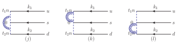
Figure 2: One loop self-energy corrections for quasi-DA.

In addition, since $n_{z}^{2}\neq 0$, the self-energy diagram of the Wilson line of the quasi-DA also contributes. These two Wilson lines give three terms of one-loop self-energy corrections which are shown in Fig. 2. Those three self-energy reads

$$\tilde{\mathcal{M}}^{j} = \frac{\alpha_{s}C_{F}}{4\pi}\tilde{S}^{(0)}\Bigg{[}\frac{\delta(x_{2}-x_{2,0})}{\sqrt{(x_{1}-x_{1,0})^{2}}}+\frac{\delta(x_{1}-x_{1,0})}{\sqrt{(x_{2}-x_{2,0})^{2}}}$$

$$-\frac{\delta(x_{3}-x_{3,0})}{\sqrt{(x_{1}-x_{1,0})^{2}}}\Bigg{]}_{\oplus},$$

$$\tilde{\mathcal{M}}^{k} = -\frac{\alpha_{s}C_{F}}{2\pi}\tilde{S}^{(0)}\Big{[}\frac{\delta(x_{2}-x_{2,0})}{\sqrt{(x_{1}-x_{1,0})^{2}}}\Big{]}_{\oplus},$$

$$\tilde{\mathcal{M}}^{l} = -\frac{\alpha_{s}C_{F}}{2\pi}\tilde{S}^{(0)}\Big{[}\frac{\delta(x_{1}-x_{1,0})}{\sqrt{(x_{2}-x_{2,0})^{2}}}\Big{]}_{\oplus}.$$ (46)

According to Eq. (III-III), after adding up all the results of one-loop quasi-DA diagrams, we find the normalized quasi-DA as

$$\tilde{\phi}(x_{1},x_{2},\mu) = \delta(x_{1}-x_{1,0})\delta(x_{2}-x_{2,0})+\frac{\alpha_{s}C_{F}}{8\pi}$$ (47)

$$\times\Bigg{\{}\Big{[}g_{2}\delta(x_{2}-x_{2,0})+g_{3}\delta(x_{3}-x_{3,0})$$

$$+\{x_{2}\leftrightarrow x_{1},x_{2,0}\leftrightarrow x_{1,0}\}\Big{]}\Bigg{\}}_{\oplus},$$

with

$$g_{2}=\left\{\begin{aligned} &\frac{\left(x_{1,0}+x_{1}\right)\left(x_{3,0}+x_{3}\right)\ln\left(-\frac{x_{3,0}-x_{3}}{x_{3}}\right)}{x_{1,0}x_{3,0}\left(x_{3,0}-x_{3}\right)}-\frac{x_{1}\left(2x_{1,0}+x_{3,0}+x_{3}\right)\ln\left(-\frac{x_{1}}{x_{3}}\right)}{x_{1,0}\left(x_{3,0}-x_{3}\right)\left(x_{1,0}+x_{3,0}\right)},~{}x_{1}<0\\ &\frac{x_{1}\left(-x_{1,0}+2x_{2,0}+x_{1}-2\right)}{\left(x_{1}-x_{1,0}\right)x_{1,0}\left(x_{2,0}-1\right)\epsilon_{\text{IR}}}+\frac{2x_{1}\ln\left(\frac{4x_{1}\left(x_{3}-x_{3,0}\right)\left(p^{z}\right)^{2}}{\mu^{2}}\right)}{x_{1,0}\left(x_{3}-x_{3,0}\right)}+\frac{x_{1}\ln\left(\frac{4x_{1}x_{3}\left(p^{z}\right)^{2}}{\mu^{2}}\right)}{x_{1,0}\left(x_{1,0}+x_{3,0}\right)}\\ &+\frac{x_{1}\left(-3x_{1,0}-2x_{3,0}+x_{1}\right)}{x_{1,0}\left(x_{3}-x_{3,0}\right)\left(x_{1,0}+x_{3,0}\right)}-\frac{\left(\left(x_{3}-x_{3,0}\right){}^{2}-2x_{3}x_{1,0}\right)\ln\left(\frac{x_{3}-x_{3,0}}{x_{3}}\right)}{x_{1,0}\left(x_{3}-x_{3,0}\right)x_{3,0}},~{}0<x_{1}<x_{1,0}\\ &\frac{x_{3}\left(-x_{1,0}-2x_{2,0}+x_{1}+2\right)}{\left(x_{1}-x_{1,0}\right)\left(x_{2,0}-1\right)x_{3,0}\epsilon_{\text{IR}}}+\frac{2x_{3}\ln\left(\frac{4x_{3}\left(x_{1}-x_{1,0}\right)\left(p^{z}\right)^{2}}{\mu^{2}}\right)}{\left(x_{1}-x_{1,0}\right)x_{3,0}}+\frac{x_{3}\ln\left(\frac{4x_{1}x_{3}\left(p^{z}\right)^{2}}{\mu^{2}}\right)}{x_{3,0}\left(x_{1,0}+x_{3,0}\right)}\\ &+\frac{x_{3}\left(-2x_{1,0}-3x_{3,0}+x_{3}\right)}{\left(x_{1}-x_{1,0}\right)x_{3,0}\left(x_{1,0}+x_{3,0}\right)}-\frac{\left(\left(x_{1}-x_{1,0}\right){}^{2}-2x_{1}x_{3,0}\right)\ln\left(\frac{x_{1}-x_{1,0}}{x_{1}}\right)}{\left(x_{1}-x_{1,0}\right)x_{1,0}x_{3,0}},~{}x_{1,0}<x_{1}<x_{1,0}+x_{3,0}\\ &\frac{\left(x_{1,0}+x_{1}\right)\left(x_{3,0}+x_{3}\right)\ln\left(-\frac{x_{3,0}-x_{3}}{x_{3}}\right)}{x_{1,0}x_{3,0}\left(x_{3,0}-x_{3}\right)}-\frac{x_{1}\left(2x_{1,0}+x_{3,0}+x_{3}\right)\ln\left(-\frac{x_{1}}{x_{3}}\right)}{x_{1,0}\left(x_{3,0}-x_{3}\right)\left(x_{1,0}+x_{3,0}\right)},~{}x_{1}>x_{1,0}+x_{3,0}\\ \end{aligned}\right.$$

$$g_{3}=\left\{\begin{aligned} &\frac{\left(x_{1,0}x_{2,0}+x_{1}x_{2}\right)\ln\left(\frac{x_{2}-x_{2,0}}{x_{2}}\right)}{x_{1,0}\left(x_{2}-x_{2,0}\right)x_{2,0}}-\frac{x_{1}\left(x_{1,0}+x_{2}\right)\ln\left(-\frac{x_{1}}{x_{2}}\right)}{x_{1,0}\left(x_{2}-x_{2,0}\right)\left(x_{1,0}+x_{2,0}\right)},~{}x_{1}<0\\ &\frac{2x_{1}\left(x_{1,0}+x_{2}\right)}{\left(x_{1}+x_{2}\right)\left(x_{1}-x_{1,0}\right)x_{1,0}\epsilon_{\text{IR}}}+\frac{x_{1}\ln\left(\frac{4x_{1}\left(x_{2}-x_{2,0}\right)\left(p^{z}\right)^{2}}{\mu^{2}}\right)}{x_{1,0}\left(x_{2}-x_{2,0}\right)}+\frac{x_{1}\ln\left(\frac{4x_{1}x_{2}\left(p^{z}\right)^{2}}{\mu^{2}}\right)}{x_{1,0}\left(x_{1,0}+x_{2,0}\right)}\\ &+\frac{1}{x_{1}-x_{1,0}}+\frac{2x_{1}+x_{2}}{x_{1,0}\left(x_{1,0}+x_{2,0}\right)}+\frac{\left(x_{1,0}\left(x_{2,0}+x_{1}\right)-x_{1}^{2}\right)\ln\left(\frac{x_{2}-x_{2,0}}{x_{2}}\right)}{x_{1,0}\left(x_{2}-x_{2,0}\right)x_{2,0}},~{}0<x_{1}<x_{1,0}\\ &\frac{2x_{2}\left(x_{2,0}+x_{1}\right)}{\left(x_{1}+x_{2}\right)\left(x_{2}-x_{2,0}\right)x_{2,0}\epsilon_{\text{IR}}}+\frac{x_{2}\ln\left(\frac{4x_{2}\left(x_{1}-x_{1,0}\right)\left(p^{z}\right)^{2}}{\mu^{2}}\right)}{\left(x_{1}-x_{1,0}\right)x_{2,0}}+\frac{x_{2}\ln\left(\frac{4x_{1}x_{2}\left(p^{z}\right)^{2}}{\mu^{2}}\right)}{x_{2,0}\left(x_{1,0}+x_{2,0}\right)}\\ &+\frac{1}{x_{2}-x_{2,0}}+\frac{x_{1}+2x_{2}}{x_{2,0}\left(x_{1,0}+x_{2,0}\right)}+\frac{\left(\left(x_{1,0}+x_{2}\right)x_{2,0}-x_{2}^{2}\right)\ln\left(\frac{x_{1}-x_{1,0}}{x_{1}}\right)}{\left(x_{1}-x_{1,0}\right)x_{1,0}x_{2,0}},~{}x_{1,0}<x_{1}<x_{1,0}+x_{2,0}\\ &\frac{\left(x_{1,0}x_{2,0}+x_{1}x_{2}\right)\ln\left(\frac{x_{1}-x_{1,0}}{x_{1}}\right)}{\left(x_{1}-x_{1,0}\right)x_{1,0}x_{2,0}}-\frac{x_{2}\left(x_{2,0}+x_{1}\right)\ln\left(-\frac{x_{2}}{x_{1}}\right)}{\left(x_{1}-x_{1,0}\right)x_{2,0}\left(x_{1,0}+x_{2,0}\right)},~{}x_{1}>x_{1,0}+x_{2,0}.\\ \end{aligned}\right.$$

There is no divergence for $x_{1}(x_{2})<0$. The expressions of the quasi-DA $\tilde{\phi}(x_{1},x_{2},\mu)$ differ by a minus sign between interval $x_{1}(x_{2})<0$ and interval $x_{1}(x_{2})>1-x_{2}(x_{1})$. The above results have infrared divergence in the other two intervals. We can find that this infrared divergence is consistent with the infrared divergence in LCDA Eq. (25), which validate the factorization assumption at one-loop order. A direct demonstration using expansion by region is shown in Appendix C.

IV off-shell results

Compared to the continuum space, the renormalization of lattice operators is a necessary ingredient to obtain physical results from numerical simulations. In the literature, it has been noticed that a regularization invariant momentum subtraction method (RI/MOM) Martinelli:1994ty can avoid the use of lattice perturbation theory and allow a non-perturbative determination of the renormalization constants of many composite operators Constantinou:2017sej ; Sturm:2009kb ; Alexandrou:2017huk ; Stewart:2017tvs ; Chen:2017mzz ; Lin:2017ani ; Liu:2018tox ; Liu:2019urm ; LatticeParton:2018gjr . In the following we also provide an analysis of the baryon distribution amplitudes in this scheme.

We calculate the quasi-DA in the space-like $p^{2}=-\rho{(p^{z})}^{2}<0$ kinematics region. Fig. 1(a) gives

$$\tilde{\mathcal{M}}^{a}_{\rm OF} = ig^{2}\frac{-C_{F}}{2}{p^{z}}^{2}\int\frac{d^{4}q}{(2\pi)^{4}}\frac{1}{q^{2}+i\epsilon}\frac{1}{(k_{3}-q)^{2}+i\epsilon}$$

$$\times\frac{\delta(x_{1}p^{z}-q^{z}-{k_{1}}^{z})\delta(x_{2}p^{z}-{k_{2}}^{z})}{(q+k_{1})^{2}+i\epsilon}$$

$$\times\left(-\frac{1}{2}\right){\rm tr}\left(\not{p}\gamma^{5}\gamma^{\mu}(\not{q}+\not{k_{1}})\gamma^{5}\gamma^{z}\right)({\not{k_{3}}}-{\not{q}})\gamma_{\mu}u(k_{3}).$$

A subtle issue for the off-shell matrix elements is that there are multiple projection ways, and here we adopt a strategy called the minimal projection LatticeParton:2018gjr . Namely, we use the trace formulae technique, and all kinds of Lorentz structures above the spinor part can be projected out:

$$\left(-\frac{1}{2}\right){\rm tr}\left(\not{p}\gamma^{5}\gamma^{\mu}(\not{q}+\not{k_{1}})\gamma^{5}\gamma^{z}\right)({\not{k_{3}}}-{\not{q}})\gamma_{\mu}u(k_{3})$$ (49)

$$= (a_{1}+a_{2}\not{n}_{t}\not{n}_{z}+a_{3}\not{n}_{\perp}\not{n}_{z}+a_{4}\not{n}_{\perp}\not{n}_{t})\tilde{S},$$

where

$$a_{1} = x_{1,0}\left({(p^{z})}^{2}\rho\left(x_{1}-x_{1,0}\right)+2p\cdot q\right)+{(p^{z})}^{2}x_{1}\rho x_{3,0}+q^{2}$$

$$a_{2} = \frac{p\cdot q\left(p^{0}x_{3,0}-q^{0}\right)}{p^{z}}-p^{z}\Big{\{}x_{1,0}\big{[}q^{0}(1-\rho)+p^{0}\left(\rho+1\right)x_{3,0}\big{]}+x_{1}\left(q^{0}-p^{0}x_{3,0}\right)+p^{0}x_{1,0}^{2}+q^{0}x_{3,0}-p^{0}x_{1}^{2}\Big{\}}$$

$$a_{3} = \frac{p\cdot q\left(q_{\perp}-p_{\perp}x_{3,0}\right)}{p^{z}}+p^{z}\Big{\{}x_{1,0}\left(p_{\perp}x_{1,0}+q_{\perp}(1-\rho)\right)+x_{3,0}\big{[}q_{\perp}+p_{\perp}\left(1+\rho\right)x_{1,0}\big{]}+x_{1}\left(q_{\perp}-p_{\perp}x_{3,0}\right)-p_{\perp}x_{1}^{2}\Big{\}}$$

$$a_{4} = \left(x_{1,0}+x_{3,0}+x_{1}\right)(p_{\perp}q^{0}-p^{0}q_{\perp}).$$ (50)

In the on-shell limit, the third and the last term $a_{3},a_{4}$ disappear after integrating out the momentum $q$, and the product $\not{n}_{t}\not{n}_{z}$ goes to a unit matrix. Therefore, the summation $a_{1}+a_{2}$ captures all terms that lead to UV divergences in the on-shell limit. This is similar to Fig. 1(b,f,g). The corresponding results are as follows

$$\tilde{\mathcal{M}}_{\rm OF}^{a}=\frac{\delta(x_{2}-x_{2,0})\alpha_{s}C_{F}}{64\pi(1-\rho)^{3/2}x_{1,0}x_{3,0}(x_{1,0}+x_{3,0})p^{z}}\tilde{S}^{(0)}$$

$$\times\left\{\begin{aligned} &\ln\left(\frac{\left(\left(\sqrt{1-\rho}+1\right)\left(x_{1,0}+x_{3,0}\right)-2x_{1}\right){}^{2}}{\left(\left(\sqrt{1-\rho}-1\right)\left(x_{1,0}+x_{3,0}\right)+2x_{1}\right){}^{2}}\right)\left(\rho\left(x_{1,0}+x_{3,0}\right){}^{2}p^{0}-4(\rho-1)x_{1}\left(x_{1,0}+x_{3,0}\right)p^{z}-4x_{1}^{2}p^{0}\right)\\ &+\ln\left(\frac{\left(\left(\sqrt{1-\rho}+1\right)x_{3,0}+2x_{1,0}-2x_{1}\right){}^{2}}{\left(\left(\sqrt{1-\rho}-1\right)x_{3,0}-2x_{1,0}+2x_{1}\right){}^{2}}\right)\\ &\times\left(4(\rho-1)\left(x_{1}-x_{1,0}\right)\left(x_{1,0}+x_{3,0}\right)p^{z}-p^{0}\left(\rho x_{3,0}\left(2x_{1,0}+x_{3,0}\right)+4x_{1}x_{1,0}-4x_{1}^{2}\right)\right)\\ &+\ln\left(\frac{\left(\left(\sqrt{1-\rho}+1\right)x_{1,0}-2x_{1}\right){}^{2}}{\left(\left(\sqrt{1-\rho}-1\right)x_{1,0}+2x_{1}\right){}^{2}}\right)\\ &\times\left(4x_{1}\left(x_{3,0}p^{0}+(\rho-1)\left(x_{1,0}+x_{3,0}\right)p^{z}\right)-\rho x_{1,0}\left(x_{1,0}+2x_{3,0}\right)p^{0}+4x_{1}^{2}p^{0}\right),~{}x_{1}<0\\ &\ln\left(\frac{\left(\left(\sqrt{1-\rho}+1\right)x_{3,0}+2x_{1,0}-2x_{1}\right){}^{2}}{\left(\left(\sqrt{1-\rho}-1\right)x_{3,0}-2x_{1,0}+2x_{1}\right){}^{2}}\right)\\ &\times\left(4(\rho-1)\left(x_{1}-x_{1,0}\right)\left(x_{1,0}+x_{3,0}\right)p^{z}-p^{0}\left(\rho x_{3,0}\left(2x_{1,0}+x_{3,0}\right)+4x_{1}x_{1,0}-4x_{1}^{2}\right)\right)\\ &+x_{3,0}p^{0}\ln\left(\frac{\left(\sqrt{1-\rho}+1\right)^{2}}{\left(\sqrt{1-\rho}-1\right)^{2}}\right)\left(\rho x_{3,0}+4x_{1}\right)-\frac{8(1-\rho)^{3/2}x_{1}x_{3,0}p^{0}}{z^{2}},~{}0<x_{1}<x_{1,0}\\ &x_{1,0}\ln\left(\frac{\left(\sqrt{1-\rho}+1\right)^{2}}{\left(\sqrt{1-\rho}-1\right)^{2}}\right)\left(p^{0}\left(\rho x_{1,0}-4x_{1}\right)-4(\rho-1)\left(x_{1,0}+x_{3,0}\right)p^{z}\right)\\ &+\ln\left(\frac{\left(\left(\sqrt{1-\rho}+1\right)x_{1,0}-2x_{1}\right){}^{2}}{\left(\left(\sqrt{1-\rho}-1\right)x_{1,0}+2x_{1}\right){}^{2}}\right)\left(4x_{1}\left(-x_{3,0}p^{0}-(\rho-1)\left(x_{1,0}+x_{3,0}\right)p^{z}\right)+\rho x_{1,0}\left(x_{1,0}+2x_{3,0}\right)p^{0}-4x_{1}^{2}p^{0}\right)\\ &-\frac{8(1-\rho)^{3/2}x_{1,0}\left(x_{1,0}+x_{3,0}-x_{1}\right)p^{0}}{z^{2}},~{}x_{1,0}<x_{1}<x_{1,0}+x_{3,0}\\ &\ln\left(\frac{\left(\left(\sqrt{1-\rho}+1\right)\left(x_{1,0}+x_{3,0}\right)-2x_{1}\right){}^{2}}{\left(\left(\sqrt{1-\rho}-1\right)\left(x_{1,0}+x_{3,0}\right)+2x_{1}\right){}^{2}}\right)\left(-\rho\left(x_{1,0}+x_{3,0}\right){}^{2}p^{0}+4(\rho-1)x_{1}\left(x_{1,0}+x_{3,0}\right)p^{z}+4x_{1}^{2}p^{0}\right)\\ &+\ln\left(\frac{\left(\left(\sqrt{1-\rho}+1\right)x_{3,0}+2x_{1,0}-2x_{1}\right){}^{2}}{\left(\left(\sqrt{1-\rho}-1\right)x_{3,0}-2x_{1,0}+2x_{1}\right){}^{2}}\right)\\ &\times\left(p^{0}\left(\rho x_{3,0}\left(2x_{1,0}+x_{3,0}\right)+4x_{1}x_{1,0}-4x_{1}^{2}\right)-4(\rho-1)\left(x_{1}-x_{1,0}\right)\left(x_{1,0}+x_{3,0}\right)p^{z}\right)\\ &+\ln\left(\frac{\left(\left(\sqrt{1-\rho}+1\right)x_{1,0}-2x_{1}\right){}^{2}}{\left(\left(\sqrt{1-\rho}-1\right)x_{1,0}+2x_{1}\right){}^{2}}\right)\\ &\times\left(4x_{1}\left(-x_{3,0}p^{0}-(\rho-1)\left(x_{1,0}+x_{3,0}\right)p^{z}\right)+\rho x_{1,0}\left(x_{1,0}+2x_{3,0}\right)p^{0}-4x_{1}^{2}p^{0}\right),~{}x_{1}>x_{1,0}+x_{3,0}\end{aligned}\right.$$

$$\tilde{\mathcal{M}}_{\rm{OF}}^{c}=\frac{\alpha_{s}C_{F}}{16\pi\sqrt{1-\rho}x_{1,0}}\tilde{S}^{(0)}$$

$$\times\left\{\begin{aligned} &\Bigg{\{}\frac{\delta(x_{2}-x_{2,0})}{x_{1}-x_{1,0}}\Big{[}\left(\rho x_{1,0}-4x_{1}\right)\ln\left(\frac{\left(\left(\sqrt{1-\rho}+1\right)x_{1,0}-2x_{1}\right){}^{2}}{\left(\left(\sqrt{1-\rho}-1\right)x_{1,0}+2x_{1}\right){}^{2}}\right)-4\sqrt{1-\rho}x_{1,0}\Big{]}\Bigg{\}}_{\oplus},~{}x_{1}<0\\ &\Bigg{\{}\frac{\delta(x_{2}-x_{2,0})}{x_{1}-x_{1,0}}\Big{[}4\sqrt{1-\rho}\left(2x_{1}-x_{1,0}\right)-\ln\left(\frac{\left(\sqrt{1-\rho}+1\right)^{2}}{\left(\sqrt{1-\rho}-1\right)^{2}}\right)\left(4x_{1}-\rho x_{1,0}\right)\Big{]}\Bigg{\}}_{\oplus},~{}0<x_{1}<x_{1,0}\\ &\Bigg{\{}\frac{\delta(x_{2}-x_{2,0})}{x_{1}-x_{1,0}}\Big{[}4\sqrt{1-\rho}x_{1,0}+\left(4x_{1}-\rho x_{1,0}\right)\ln\left(\frac{\left(\left(\sqrt{1-\rho}+1\right)x_{1,0}-2x_{1}\right){}^{2}}{\left(\left(\sqrt{1-\rho}-1\right)x_{1,0}+2x_{1}\right){}^{2}}\right)\Big{]}\Bigg{\}}_{\oplus},~{}x_{1}>x_{1,0}\\ \end{aligned}\right.$$

$$\tilde{\mathcal{M}}_{\rm{OF}}^{d}=\frac{\delta(x_{3}-x_{3,0})\alpha_{s}C_{F}}{8\pi\sqrt{1-\rho}x_{1,0}x_{2,0}(x_{1,0}+x_{2,0})}\tilde{S}^{(0)}$$

$$\times\left\{\begin{aligned} &x_{1}x_{2,0}\ln\left(\frac{\left(\left(\sqrt{1-\rho}+1\right)x_{1,0}-2x_{1}\right){}^{2}}{\left(\left(\sqrt{1-\rho}-1\right)x_{1,0}+2x_{1}\right){}^{2}}\right)\\ &+x_{1,0}\left(x_{1,0}+x_{2,0}-x_{1}\right)\ln\left(\frac{\left(\left(\sqrt{1-\rho}+1\right)x_{2,0}+2x_{1,0}-2x_{1}\right){}^{2}}{\left(\left(\sqrt{1-\rho}-1\right)x_{2,0}-2x_{1,0}+2x_{1}\right){}^{2}}\right),~{}x_{1}<0\\ &x_{1}x_{2,0}\ln\left(\frac{\left(\sqrt{1-\rho}+1\right)^{2}}{\left(\sqrt{1-\rho}-1\right)^{2}}\right)\\ &+x_{1,0}\left(x_{1,0}+x_{2,0}-x_{1}\right)\ln\left(\frac{\left(\left(\sqrt{1-\rho}+1\right)x_{2,0}+2x_{1,0}-2x_{1}\right){}^{2}}{\left(\left(\sqrt{1-\rho}-1\right)x_{2,0}-2x_{1,0}+2x_{1}\right){}^{2}}\right),~{}0<x_{1}<x_{1,0}\\ &x_{1,0}\left(x_{1,0}+x_{2,0}-x_{1}\right)\ln\left(\frac{\left(\sqrt{1-\rho}+1\right)^{2}}{\left(\sqrt{1-\rho}-1\right)^{2}}\right)\\ &-x_{1}x_{2,0}\ln\left(\frac{\left(\left(\sqrt{1-\rho}+1\right)x_{1,0}-2x_{1}\right){}^{2}}{\left(\left(\sqrt{1-\rho}-1\right)x_{1,0}+2x_{1}\right){}^{2}}\right),~{}x_{1,0}<x_{1}<x_{1,0}+x_{2,0}\\ &x_{1}x_{2,0}\left(-\ln\left(\frac{\left(\left(\sqrt{1-\rho}+1\right)x_{1,0}-2x_{1}\right){}^{2}}{\left(\left(\sqrt{1-\rho}-1\right)x_{1,0}+2x_{1}\right){}^{2}}\right)\right)\\ &-x_{1,0}\left(x_{1,0}+x_{2,0}-x_{1}\right)\ln\left(\frac{\left(\left(\sqrt{1-\rho}+1\right)x_{2,0}+2x_{1,0}-2x_{1}\right){}^{2}}{\left(\left(\sqrt{1-\rho}-1\right)x_{2,0}-2x_{1,0}+2x_{1}\right){}^{2}}\right),~{}x_{1}>x_{1,0}+x_{2,0}\\ \end{aligned}\right.$$

$$\tilde{\mathcal{M}}_{\rm{OF}}^{f}=\frac{\alpha_{s}C_{F}}{32\pi\left(1-\rho\right)^{3/2}x_{3,0}p^{z}}\tilde{S}^{(0)}$$

$$\times\left\{\begin{aligned} &\Bigg{\{}\frac{\delta(x_{2}-x_{2,0})}{x_{1}-x_{1,0}}\Big{[}\ln\left(\frac{\left(\left(\sqrt{1-\rho}+1\right)x_{3,0}+2x_{1,0}-2x_{1}\right){}^{2}}{\left(\left(\sqrt{1-\rho}-1\right)x_{3,0}-2x_{1,0}+2x_{1}\right){}^{2}}\right)\\ &\times\left(x_{3,0}\left(p^{0}-(\rho-1)\left(p^{0}+2p^{z}\right)\right)-2\left(x_{1}-x_{1,0}\right)\left(p^{0}-(\rho-1)p^{z}\right)\right)-\frac{4(1-\rho)^{3/2}x_{3,0}p^{0}}{z^{2}}\Big{]}\Bigg{\}}_{\oplus},~{}x_{1}<x_{1,0}\\ &\Bigg{\{}\frac{\delta(x_{2}-x_{2,0})}{x_{1}-x_{1,0}}\Big{[}\frac{4(1-\rho)^{3/2}\left(-2x_{1,0}-x_{3,0}+2x_{1}\right)p^{0}}{z^{2}}-\ln\left(\frac{\left(\sqrt{1-\rho}+1\right)^{2}}{\left(\sqrt{1-\rho}-1\right)^{2}}\right)\\ &\times\left(2\left(x_{1}-x_{1,0}\right)\left(p^{0}-(\rho-1)p^{z}\right)+x_{3,0}\left((\rho-2)p^{0}+2(\rho-1)p^{z}\right)\right)\Big{]}\Bigg{\}}_{\oplus},~{}x_{1,0}<x_{1}<x_{1,0}+x_{3,0}\\ &\Bigg{\{}\frac{\delta(x_{2}-x_{2,0})}{x_{1}-x_{1,0}}\Big{[}\ln\left(\frac{\left(\left(\sqrt{1-\rho}+1\right)x_{3,0}+2x_{1,0}-2x_{1}\right){}^{2}}{\left(\left(\sqrt{1-\rho}-1\right)x_{3,0}-2x_{1,0}+2x_{1}\right){}^{2}}\right)\\ &\times\left(2\left(x_{1}-x_{1,0}\right)\left(p^{0}-(\rho-1)p^{z}\right)+x_{3,0}\left((\rho-2)p^{0}+2(\rho-1)p^{z}\right)\right)+\frac{4(1-\rho)^{3/2}x_{3,0}p^{0}}{z^{2}}\Big{]}\Bigg{\}}_{\oplus},~{}x_{1}>x_{1,0}+x_{3,0}\\ \end{aligned}\right.$$

$$\tilde{\mathcal{M}}_{\rm{OF}}^{h}=\frac{\alpha_{s}C_{F}}{32\pi\sqrt{1-\rho}x_{1,0}}\tilde{S}^{(0)}$$

$$\times\left\{\begin{aligned} &\Bigg{\{}\frac{\delta(x_{2}-x_{2,0})-\delta(x_{3}-x_{3,0})}{x_{1,0}-x_{1}}\Big{[}\left(\rho x_{1,0}-4x_{1}\right)\ln\left(\frac{\left(\left(\sqrt{1-\rho}+1\right)x_{1,0}-2x_{1}\right){}^{2}}{\left(\left(\sqrt{1-\rho}-1\right)x_{1,0}+2x_{1}\right){}^{2}}\right)-4\sqrt{1-\rho}x_{1,0}\Big{]}\Bigg{\}}_{\oplus},~{}x_{1}<0\\ &\Bigg{\{}\frac{\delta(x_{2}-x_{2,0})-\delta(x_{3}-x_{3,0})}{x_{1,0}-x_{1}}4\sqrt{1-\rho}\left(2x_{1}-x_{1,0}\right)+\ln\left(\frac{\left(\sqrt{1-\rho}+1\right)^{2}}{\left(\sqrt{1-\rho}-1\right)^{2}}\right)\left(\rho x_{1,0}-4x_{1}\right)\Big{]}\Bigg{\}}_{\oplus},~{}0<x_{1}<x_{1,0}\\ &\Bigg{\{}\frac{\delta(x_{2}-x_{2,0})-\delta(x_{3}-x_{3,0})}{x_{1,0}-x_{1}}4\sqrt{1-\rho}x_{1,0}+\left(4x_{1}-\rho x_{1,0}\right)\ln\left(\frac{\left(\left(\sqrt{1-\rho}+1\right)x_{1,0}-2x_{1}\right){}^{2}}{\left(\left(\sqrt{1-\rho}-1\right)x_{1,0}+2x_{1}\right){}^{2}}\right)\Big{]}\Bigg{\}}_{\oplus},~{}x_{1}>x_{1,0}\\ \end{aligned}\right.$$

$$\tilde{\mathcal{M}}_{\rm{OF}}^{b} = \tilde{\mathcal{M}}_{\rm{OF}}^{a}|_{x_{2}\leftrightarrow x_{1},x_{2,0}\leftrightarrow x_{1,0}},$$

$$\tilde{\mathcal{M}}_{\rm{OF}}^{e} = \tilde{\mathcal{M}}_{\rm{OF}}^{c}|_{x_{2}\leftrightarrow x_{1},x_{2,0}\leftrightarrow x_{1,0}},$$

$$\tilde{\mathcal{M}}_{\rm{OF}}^{g} = \tilde{\mathcal{M}}_{\rm{OF}}^{f}|_{x_{2}\leftrightarrow x_{1},x_{2,0}\leftrightarrow x_{1,0}},$$

$$\tilde{\mathcal{M}}_{\rm{OF}}^{i} = \tilde{\mathcal{M}}_{\rm{OF}}^{h}|_{x_{2}\leftrightarrow x_{1},x_{2,0}\leftrightarrow x_{1,0}},$$ (51)

$$\tilde{\mathcal{M}}_{\rm{OF}}^{j,k,l}=\tilde{\mathcal{M}}^{j,k,l}.$$ (52)

The subscript “$\rm OF$” indicates the off-shell case. We have found that the self-energy correction of the Wilson line is independent of whether the momentum of the external leg is on-shell or not. Finally, the off-shell quasi-DA up to one-loop accuracy is given as

$$\tilde{\phi}(x_{1},x_{2},\mu)_{\rm OF} = \delta(x_{1}-x_{1,0})\delta(x_{2}-x_{2,0})+\frac{\alpha_{s}C_{F}}{8\pi}$$ (53)

$$\times\Bigg{\{}\Big{[}g^{\prime}_{2}\delta(x_{2}-x_{2,0})+g^{\prime}_{3}\delta(x_{3}-x_{3,0})$$

$$+\{x_{2}\leftrightarrow x_{1},x_{2,0}\leftrightarrow x_{1,0}\}\Big{]}\Bigg{\}}_{\oplus},$$

with

$$g^{\prime}_{2}=\frac{1}{8p^{z}(1-\rho)^{5/2}(x_{1}-x_{1,0})x_{1,0}x_{3,0}(x_{1,0}+x_{3,0})}$$

$$\times\left\{\begin{aligned} &-8(1-\rho)^{3/2}x_{1,0}x_{3,0}\left(x_{1,0}+x_{3,0}\right)\left(p^{0}+(\rho-1)p^{z}\right)-(1-\rho)\left(x_{1}-x_{1,0}\right)\ln\left(\frac{\left(\left(\sqrt{1-\rho}+1\right)\left(x_{1,0}+x_{3,0}\right)-2x_{1}\right){}^{2}}{\left(\left(\sqrt{1-\rho}-1\right)\left(x_{1,0}+x_{3,0}\right)+2x_{1}\right){}^{2}}\right)\\ &\times\Big{[}-\rho\left(x_{1,0}+x_{3,0}\right){}^{2}p^{0}+4(\rho-1)x_{1}\left(x_{1,0}+x_{3,0}\right)p^{z}+4x_{1}^{2}p^{0}\Big{]}-(1-\rho)\ln\left(\frac{\left(\left(\sqrt{1-\rho}+1\right)x_{1,0}-2x_{1}\right){}^{2}}{\left(\left(\sqrt{1-\rho}-1\right)x_{1,0}+2x_{1}\right){}^{2}}\right)\\ &\times\Big{\{}2(\rho-1)x_{3,0}\left(x_{1,0}+x_{3,0}\right)\left(\rho x_{1,0}-4x_{1}\right)p^{z}-\left(x_{1}-x_{1,0}\right)\Big{[}4x_{1}\left(x_{3,0}p^{0}+(\rho-1)\left(x_{1,0}+x_{3,0}\right)p^{z}\right)\\ &-\rho x_{1,0}\left(x_{1,0}+2x_{3,0}\right)p^{0}+4x_{1}^{2}p^{0}\Big{]}\Big{\}}-(1-\rho)\ln\left(\frac{\left(\left(\sqrt{1-\rho}+1\right)x_{3,0}+2x_{1,0}-2x_{1}\right){}^{2}}{\left(\left(\sqrt{1-\rho}-1\right)x_{3,0}-2x_{1,0}+2x_{1}\right){}^{2}}\right)\\ &\times\Big{\{}2x_{1,0}\left(x_{1,0}+x_{3,0}\right)\Big{[}x_{3,0}\left((\rho-2)p^{0}+2(\rho-1)p^{z}\right)+2\left(x_{1}-x_{1,0}\right)\left(p^{0}-\rho p^{z}+p^{z}\right)\Big{]}-\left(x_{1}-x_{1,0}\right)\\ &\times\Big{[}4\left(x_{1}-x_{1,0}\right)\left((\rho-1)x_{1,0}p^{z}+x_{1}p^{0}\right)+2x_{3,0}\left(2(\rho-1)x_{1}p^{z}-x_{1,0}\left(\rho p^{0}+2(\rho-1)p^{z}\right)\right)-\rho x_{3,0}^{2}p^{0}\Big{]}\Big{\}},~{}x_{1}<0\\ &-8(1-\rho)^{3/2}x_{3,0}\left(x_{1,0}\left(x_{1,0}+x_{3,0}\right)\left(p^{0}-(1-\rho)p^{z}\right)-x_{1}\left(x_{1,0}\left(p^{0}+2(1-\rho)p^{z}\right)+2(1-\rho)x_{3,0}p^{z}\right)+x_{1}^{2}p^{0}\right)\\ &+(1-\rho)x_{3,0}\ln\left(\frac{\left(\sqrt{1-\rho}+1\right)^{2}}{\left(\sqrt{1-\rho}-1\right)^{2}}\right)\Bigg{\{}-\rho x_{1,0}\Bigg{[}x_{3,0}p^{0}+2(\rho-1)\left(x_{1,0}+x_{3,0}\right)p^{z}\Bigg{]}+x_{1}\Bigg{[}x_{3,0}\left(\rho p^{0}+8(\rho-1)p^{z}\right)\\ &-4x_{1,0}\left(p^{0}-2(\rho-1)p^{z}\right)\Bigg{]}+4x_{1}^{2}p^{0}\Bigg{\}}+(1-\rho)\ln\left(\frac{\left(\left(\sqrt{1-\rho}+1\right)x_{3,0}+2x_{1,0}-2x_{1}\right){}^{2}}{\left(\left(\sqrt{1-\rho}-1\right)x_{3,0}-2x_{1,0}+2x_{1}\right){}^{2}}\right)\\ &\times\Bigg{\{}-x_{1}\Bigg{[}2x_{1,0}x_{3,0}\left((\rho+2)p^{0}+2(\rho-1)p^{z}\right)+\rho x_{3,0}^{2}p^{0}+4(\rho-1)x_{1,0}^{2}p^{z}\Bigg{]}-4x_{1}^{2}\Bigg{[}x_{1,0}\left(2p^{0}-\rho p^{z}+p^{z}\right)-(\rho-1)x_{3,0}p^{z}\Bigg{]}\\ &+x_{1,0}\Bigg{[}4x_{1,0}x_{3,0}\left(2p^{0}-\rho p^{z}+p^{z}\right)+x_{3,0}^{2}\left(4\left(p^{0}+p^{z}\right)-\rho\left(p^{0}+4p^{z}\right)\right)+4x_{1,0}^{2}p^{0}\Bigg{]}+4x_{1}^{3}p^{0}\Bigg{\}},~{}0<x_{1}<x_{1,0}\\ &-8(1-\rho)^{3/2}x_{1,0}\left(\left(x_{1,0}+x_{3,0}\right)\left(x_{3,0}\left(p^{0}+(1-\rho)p^{z}\right)+x_{1,0}p^{0}\right)-x_{1}x_{3,0}p^{0}-x_{1}^{2}p^{0}\right)-(1-\rho)x_{1,0}\ln\left(\frac{\left(\sqrt{1-\rho}+1\right)^{2}}{\left(\sqrt{1-\rho}-1\right)^{2}}\right)\\ &\times\Bigg{\{}2x_{1,0}x_{3,0}\Bigg{[}(\rho-4)p^{0}+2(\rho-1)p^{z}\Bigg{]}+2x_{3,0}^{2}\Bigg{[}(\rho-2)p^{0}+2(\rho-1)p^{z}\Bigg{]}+(\rho-4)x_{1,0}^{2}p^{0}+x_{1}p^{0}\left(4x_{3,0}-\rho x_{1,0}\right)+4x_{1}^{2}p^{0}\Bigg{\}}\\ &+(1-\rho)\ln\left(\frac{\left(\left(\sqrt{1-\rho}+1\right)x_{1,0}-2x_{1}\right){}^{2}}{\left(\left(\sqrt{1-\rho}-1\right)x_{1,0}+2x_{1}\right){}^{2}}\right)\Bigg{\{}2(\rho-1)x_{3,0}\left(x_{1,0}+x_{3,0}\right)\left(\rho x_{1,0}-4x_{1}\right)p^{z}\\ &-\left(x_{1}-x_{1,0}\right)\Bigg{[}4x_{1}\left(x_{3,0}p^{0}+(\rho-1)\left(x_{1,0}+x_{3,0}\right)p^{z}\right)-\rho x_{1,0}\left(x_{1,0}+2x_{3,0}\right)p^{0}+4x_{1}^{2}p^{0}\Bigg{]}\Bigg{\}},~{}x_{1,0}<x_{1}<x_{1,0}+x_{3,0}\\ &8(1-\rho)^{3/2}x_{1,0}x_{3,0}\left(x_{1,0}+x_{3,0}\right)\left(p^{0}-(1-\rho)p^{z}\right)+(1-\rho)\left(x_{1}-x_{1,0}\right)\ln\left(\frac{\left(\left(\sqrt{1-\rho}+1\right)\left(x_{1,0}+x_{3,0}\right)-2x_{1}\right){}^{2}}{\left(\left(\sqrt{1-\rho}-1\right)\left(x_{1,0}+x_{3,0}\right)+2x_{1}\right){}^{2}}\right)\\ &\times\Bigg{[}-\rho\left(x_{1,0}+x_{3,0}\right){}^{2}p^{0}+4(\rho-1)x_{1}\left(x_{1,0}+x_{3,0}\right)p^{z}+4x_{1}^{2}p^{0}\Bigg{]}+(1-\rho)\ln\left(\frac{\left(\left(\sqrt{1-\rho}+1\right)x_{1,0}-2x_{1}\right){}^{2}}{\left(\left(\sqrt{1-\rho}-1\right)x_{1,0}+2x_{1}\right){}^{2}}\right)\\ &\times\Bigg{\{}2(\rho-1)x_{3,0}\left(x_{1,0}+x_{3,0}\right)\left(\rho x_{1,0}-4x_{1}\right)p^{z}-\left(x_{1}-x_{1,0}\right)\Bigg{[}4x_{1}\left(x_{3,0}p^{0}+(\rho-1)\left(x_{1,0}+x_{3,0}\right)p^{z}\right)\\ &-\rho x_{1,0}\left(x_{1,0}+2x_{3,0}\right)p^{0}+4x_{1}^{2}p^{0}\Bigg{]}\Bigg{\}}+(1-\rho)\ln\left(\frac{\left(\left(\sqrt{1-\rho}+1\right)x_{3,0}+2x_{1,0}-2x_{1}\right){}^{2}}{\left(\left(\sqrt{1-\rho}-1\right)x_{3,0}-2x_{1,0}+2x_{1}\right){}^{2}}\right)\Bigg{\{}2x_{1,0}\left(x_{1,0}+x_{3,0}\right)\\ &\times\Bigg{[}x_{3,0}\left((\rho-2)p^{0}+2(\rho-1)p^{z}\right)+2\left(x_{1}-x_{1,0}\right)\left(p^{0}-\rho p^{z}+p^{z}\right)\Bigg{]}-\left(x_{1}-x_{1,0}\right)\Bigg{[}4\left(x_{1}-x_{1,0}\right)\left((\rho-1)x_{1,0}p^{z}+x_{1}p^{0}\right)\\ &-2x_{3,0}\left(x_{1,0}\left(\rho p^{0}+2(\rho-1)p^{z}\right)-2(\rho-1)x_{1}p^{z}\right)-\rho x_{3,0}^{2}p^{0}\Bigg{]}\Bigg{\}},~{}x_{1}>x_{1,0}+x_{3,0}\\ \end{aligned}\right.$$

$$g^{\prime}_{3}=\frac{1}{4\sqrt{1-\rho}(x_{1,0}+x_{2,0})x_{1,0}x_{2,0}(x_{1}-x_{1,0})}$$

$$\times\left\{\begin{aligned} &4x_{2}\left(x_{1}-x_{1,0}\right)x_{1,0}\ln\left(\frac{\left(\left(\sqrt{1-\rho}+1\right)x_{2,0}+2x_{1,0}-2x_{1}\right){}^{2}}{\left(\left(\sqrt{1-\rho}-1\right)x_{2,0}-2x_{1,0}+2x_{1}\right){}^{2}}\right)+\left(x_{1,0}+x_{2,0}\right)x_{1,0}\left(\rho x_{2,0}-4x_{2}\right)\\ &\times\ln\left(\frac{\left(\left(\sqrt{1-\rho}+1\right)x_{2,0}-2x_{2}\right){}^{2}}{\left(\left(\sqrt{1-\rho}-1\right)x_{2,0}+2x_{2}\right){}^{2}}\right)+x_{2,0}\left(\rho x_{1,0}\left(x_{1,0}+x_{2,0}\right)-4x_{1}\left(2x_{1,0}+x_{2,0}\right)+4x_{1}^{2}\right)\\ &\times\ln\left(\frac{\left(\left(\sqrt{1-\rho}+1\right)x_{1,0}-2x_{1}\right){}^{2}}{\left(\left(\sqrt{1-\rho}-1\right)x_{1,0}+2x_{1}\right){}^{2}}\right),~{}x_{1}<0\\ &8\sqrt{1-\rho}x_{1}x_{2,0}\left(x_{1,0}+x_{2,0}\right)+4x_{2}\left(x_{1}-x_{1,0}\right)x_{1,0}\ln\left(\frac{\left(\left(\sqrt{1-\rho}+1\right)x_{2,0}+2x_{1,0}-2x_{1}\right){}^{2}}{\left(\left(\sqrt{1-\rho}-1\right)x_{2,0}-2x_{1,0}+2x_{1}\right){}^{2}}\right)\\ &+\left(x_{1,0}+x_{2,0}\right)x_{1,0}\left(\rho x_{2,0}-4x_{2}\right)\ln\left(\frac{\left(\left(\sqrt{1-\rho}+1\right)x_{2,0}-2x_{2}\right){}^{2}}{\left(\left(\sqrt{1-\rho}-1\right)x_{2,0}+2x_{2}\right){}^{2}}\right)\\ &+x_{2,0}\ln\left(\frac{\left(\sqrt{1-\rho}+1\right)^{2}}{\left(\sqrt{1-\rho}-1\right)^{2}}\right)\left(\rho x_{1,0}\left(x_{1,0}+x_{2,0}\right)-4x_{1}\left(2x_{1,0}+x_{2,0}\right)+4x_{1}^{2}\right),~{}0<x_{1}<x_{1,0}\\ &-8\sqrt{1-\rho}x_{2}x_{1,0}\left(x_{1,0}+x_{2,0}\right)+x_{1,0}\ln\left(\frac{\left(\sqrt{1-\rho}+1\right)^{2}}{\left(\sqrt{1-\rho}-1\right)^{2}}\right)\left(4x_{1}\left(x_{2}-x_{2,0}\right)-(\rho-4)x_{2,0}\left(x_{1,0}+x_{2,0}\right)\right)\\ &-x_{2,0}\left(\rho x_{1,0}\left(x_{1,0}+x_{2,0}\right)-4x_{1}\left(2x_{1,0}+x_{2,0}\right)+4x_{1}^{2}\right)\ln\left(\frac{\left(\left(\sqrt{1-\rho}+1\right)x_{1,0}-2x_{1}\right){}^{2}}{\left(\left(\sqrt{1-\rho}-1\right)x_{1,0}+2x_{1}\right){}^{2}}\right),~{}x_{1,0}<x_{1}<x_{1,0}+x_{2,0}\\ &-4\left(x_{1}-x_{1,0}\right)x_{1,0}\left(x_{1,0}+x_{2,0}-x_{1}\right)\ln\left(\frac{\left(\left(\sqrt{1-\rho}+1\right)x_{2,0}+2x_{1,0}-2x_{1}\right){}^{2}}{\left(\left(\sqrt{1-\rho}-1\right)x_{2,0}-2x_{1,0}+2x_{1}\right){}^{2}}\right)\\ &+\frac{\left(x_{1}-x_{1,0}\right)x_{1,0}\left(x_{1,0}+x_{2,0}\right)\left(\rho x_{2,0}-4x_{2}\right)\ln\left(\frac{\left(\left(\sqrt{1-\rho}+1\right)x_{2,0}-2x_{2}\right){}^{2}}{\left(\left(\sqrt{1-\rho}-1\right)x_{2,0}+2x_{2}\right){}^{2}}\right)}{x_{2}-x_{2,0}}\\ &-x_{2,0}\left(\rho x_{1,0}\left(x_{1,0}+x_{2,0}\right)-4x_{1}\left(2x_{1,0}+x_{2,0}\right)+4x_{1}^{2}\right)\ln\left(\frac{\left(\left(\sqrt{1-\rho}+1\right)x_{1,0}-2x_{1}\right){}^{2}}{\left(\left(\sqrt{1-\rho}-1\right)x_{1,0}+2x_{1}\right){}^{2}}\right),~{}x_{1}>x_{1,0}+x_{2,0}.\\ \end{aligned}\right.$$

V matching kernel

In the large momentum $p^{z}\gg\Lambda_{\rm QCD}$ limit, the quasi observables can be factorized as a convolution of a perturbatively calculable matching coefficient and the corresponding light-cone observable up to power corrections suppressed by $\big{(}\frac{1}{x_{1}p^{z}},\frac{1}{x_{2}p^{z}},\frac{1}{(1-x_{1}-x_{2})p^{z}}\big{)}$. Through this factorization, one can extract light-cone observables from quasi-ones calculated on the lattice. The matching of quasi-DA and LCDA is given as

$$\tilde{\Phi}(x_{1},x_{2},\mu) = \int dy_{1}dy_{2}\mathcal{C}(x_{1},x_{2},y_{1},y_{2},\mu)\Phi(y_{1},y_{2},\mu)$$

$$+\mathcal{O}\Big{(}\frac{1}{x_{1}p^{z}},\frac{1}{x_{2}p^{z}},\frac{1}{(1-x_{1}-x_{2})p^{z}}\Big{)}.$$

With the results presented in the previous sections, one can easily obtain the matching kernel in the ${\overline{\rm MS}}$ scheme up to one-loop level

$$\mathcal{C}(x_{1},x_{2},y_{1},y_{2},\mu) = \delta(x_{1}-y_{1})\delta(x_{2}-y_{2})+\frac{\alpha_{s}C_{F}}{8\pi}$$

$$\times\Bigg{[}C_{2}(x_{1},x_{2},y_{1},y_{2})\delta(x_{2}-y_{2})$$

$$+C_{3}(x_{1},x_{2},y_{1},y_{2})\delta(x_{3}-y_{3})$$

$$+\{x_{1}\leftrightarrow x_{2},y_{1}\leftrightarrow y_{2}\}\Bigg{]}_{\oplus},$$

where $y_{3}=1-y_{1}-y_{2}$ and

$$C_{2}(x_{1},x_{2},y_{1},y_{2})=$$

$$\left\{\begin{aligned} &\frac{\left(x_{1}+y_{1}\right)\left(x_{3}+y_{3}\right)\ln\frac{y_{1}-x_{1}}{-x_{1}}}{y_{1}\left(y_{1}-x_{1}\right)y_{3}}-\frac{x_{3}\left(x_{1}+y_{1}+2y_{3}\right)\ln\frac{x_{3}}{-x_{1}}}{\left(y_{1}-x_{1}\right)y_{3}\left(y_{1}+y_{3}\right)},~{}x_{1}<0\\ &\frac{\left(x_{1}-3y_{1}-2y_{3}\right)x_{1}}{y_{1}\left(x_{3}-y_{3}\right)\left(y_{1}+y_{3}\right)}-\frac{\left[\left(x_{3}-y_{3}\right)^{2}-2x_{3}y_{1}\right]\ln\frac{x_{3}-y_{3}}{x_{3}}}{y_{1}\left(x_{3}-y_{3}\right)y_{3}}+\frac{2x_{1}\ln\frac{4x_{1}\left(x_{3}-y_{3}\right)p_{z}^{2}}{\mu^{2}}}{y_{1}\left(x_{3}-y_{3}\right)}+\frac{x_{1}\ln\frac{4x_{1}x_{3}p_{z}^{2}}{\mu^{2}}}{y_{1}\left(y_{1}+y_{3}\right)},~{}0<x_{1}<y_{1}\\ &\frac{\left(x_{3}-2y_{1}-3y_{3}\right)x_{3}}{y_{3}\left(x_{1}-y_{1}\right)\left(y_{1}+y_{3}\right)}-\frac{\left[\left(x_{1}-y_{1}\right)^{2}-2x_{1}y_{3}\right]\ln\frac{x_{1}-y_{1}}{x_{1}}}{\left(x_{1}-y_{1}\right)y_{1}y_{3}}+\frac{2x_{3}\ln\frac{4x_{3}\left(x_{1}-y_{1}\right)p_{z}^{2}}{\mu^{2}}}{\left(x_{1}-y_{1}\right)y_{3}}+\frac{x_{3}\ln\frac{4x_{1}x_{3}p_{z}^{2}}{\mu^{2}}}{y_{3}\left(y_{1}+y_{3}\right)},~{}y_{1}<x_{1}<y_{1}+y_{3}\\ &\frac{\left(x_{1}+y_{1}\right)\left(x_{3}+y_{3}\right)\ln\frac{y_{3}-x_{3}}{-x_{3}}}{y_{1}y_{3}\left(y_{3}-x_{3}\right)}-\frac{x_{1}\left(x_{3}+2y_{1}+y_{3}\right)\ln\frac{x_{1}}{-x_{3}}}{y_{1}\left(y_{3}-x_{3}\right)\left(y_{1}+y_{3}\right)},~{}x_{1}>y_{1}+y_{3}\\ \end{aligned}\right.$$

$$C_{3}(x_{1},x_{2},y_{1},y_{2})=$$ (56)

$$\left\{\begin{aligned} &\frac{\left(x_{1}x_{2}+y_{1}y_{2}\right)\ln\frac{x_{2}-y_{2}}{x_{2}}}{y_{1}\left(x_{2}-y_{2}\right)y_{2}}-\frac{x_{1}\left(x_{2}+y_{1}\right)\ln\frac{-x_{1}}{x_{2}}}{y_{1}\left(x_{2}-y_{2}\right)\left(y_{1}+y_{2}\right)},~{}x_{1}<0\\ &\frac{1}{x_{1}-y_{1}}+\frac{2x_{1}+x_{2}}{y_{1}\left(y_{1}+y_{2}\right)}+\frac{\left[\left(x_{1}+y_{2}\right)y_{1}-x_{1}{}^{2}\right]\ln\frac{x_{2}-y_{2}}{x_{2}}}{y_{1}\left(x_{2}-y_{2}\right)y_{2}}+\frac{x_{1}\ln\frac{4x_{1}\left(x_{2}-y_{2}\right)p_{z}^{2}}{\mu^{2}}}{y_{1}\left(x_{2}-y_{2}\right)}+\frac{x_{1}\ln\frac{4x_{1}x_{2}p_{z}^{2}}{\mu^{2}}}{y_{1}\left(y_{1}+y_{2}\right)},~{}0<x_{1}<y_{1}\\ &\frac{1}{x_{2}-y_{2}}+\frac{x_{1}+2x_{2}}{y_{2}\left(y_{1}+y_{2}\right)}+\frac{\left[\left(x_{2}+y_{1}\right)y_{2}-x_{2}{}^{2}\right]\ln\frac{x_{1}-y_{1}}{x_{1}}}{\left(x_{1}-y_{1}\right)y_{1}y_{2}}+\frac{x_{2}\ln\frac{4x_{2}\left(x_{1}-y_{1}\right)p_{z}^{2}}{\mu^{2}}}{\left(x_{1}-y_{1}\right)y_{2}}+\frac{x_{2}\ln\frac{4x_{1}x_{2}p_{z}^{2}}{\mu^{2}}}{y_{2}\left(y_{1}+y_{2}\right)},~{}y_{1}<x_{1}<y_{1}+y_{2}\\ &\frac{\left(x_{1}x_{2}+y_{1}y_{2}\right)\ln\frac{x_{1}-y_{1}}{x_{1}}}{y_{1}\left(x_{1}-y_{1}\right)y_{2}}-\frac{x_{2}\left(x_{1}+y_{2}\right)\ln\frac{-x_{2}}{x_{1}}}{y_{2}\left(x_{1}-y_{1}\right)\left(y_{1}+y_{2}\right)},~{}x_{1}>y_{1}+y_{2}.\\ \end{aligned}\right.$$

If we integrate over the physical region of the momentum fraction $y_{1,2}$ of the matching kernel, we find that the integral diverges. In order to eliminate this ultraviolet divergence and renormalize the lattice operators, we need a suitable renormalization of the quasi-DA $\tilde{\phi}(x_{1},x_{2},\mu)$. In the RI/MOM scheme, this is given as

$$\tilde{\phi}(x_{1},x_{2},\mu)_{\rm RI/MOM}=\frac{\tilde{\phi}(x_{1},x_{2},\mu)}{\tilde{\phi}(x_{1},x_{2},\mu)_{\rm OF}}.$$ (58)

Therefore, the renormalized matching coefficient $\mathcal{C}$ in Eq. (V) is

$$\mathcal{C}^{\mathcal{R}}(x_{1},x_{2},y_{1},y_{2},\mu) = \delta(x_{1}-y_{1})\delta(x_{2}-y_{2})+\frac{\alpha_{s}C_{F}}{8\pi}$$ (59)

$$\times\Bigg{[}C^{\prime}_{2}(x_{1},x_{2},y_{1},y_{2})\delta(x_{2}-y_{2})$$

$$+C^{\prime}_{3}(x_{1},x_{2},y_{1},y_{2})\delta(x_{3}-y_{3})$$

$$+\{x_{1}\leftrightarrow x_{2},y_{1}\leftrightarrow y_{2}\}\Bigg{]}_{\oplus},$$

where $C^{\prime}_{2}=C_{2}-g^{\prime}_{2}|_{x_{1,0}\rightarrow y_{1},x_{2,0}\rightarrow y_{2}}$ and $C^{\prime}_{3}=C_{3}-g^{\prime}_{3}|_{x_{1,0}\rightarrow y_{1},x_{2,0}\rightarrow y_{2}}$. In the RI/MOM scheme, the UV divergence in the quasi-DAs can be removed by the renormalization constant determined nonperturbatively.

It should be emphasized that although in the above calculation, an off-shell result is used to remove the UV divergences in the integration, additional infrared effects are likely to be introduced. Recently, hybrid renormalization and self-renormalization schemes have been adopted to obtain a more coherent result Ji:2020brr ; LatticePartonCollaborationLPC:2021xdx ; Chou:2022drv ; Zhang:2022xuw . The hybrid renormalization scheme treats the short-distance and long-distance renormalization separately while the self-renormalization scheme aims to extract the linear divergence by the zero-momentum matrix element. An analysis of the renormalization of the baryon quasi-DA in such a scheme is undergoing. More recently, a newly proposed method is also shown in Ref. Constantinou:2022aij .

VI Summary

In this work, we have pointed out that LCDAs of a light baryon can be obtained through a simulation of a quasi-distribution amplitude calculable on lattice QCD under the framework of large-momentum effective theory. We have calculated the one-loop perturbative contributions to LCDA and quasi-distribution amplitudes and explicitly have demonstrated the factorization of quasi-distribution amplitudes at the one-loop level. A direct analysis using expansion by region also verifies the factorizability of quasi-DA. Based on the perturbative results, we have derived the matching kernel.

For the renormalization of quasi-distribution amplitudes, we have adopted the simplest procedure at this stage and subtracted the results with an off-shell parton state as a RI/MOM result. Our result provides a first step to obtaining the LCDA from first principle lattice QCD calculations in the future. An improved renormalization procedure might be performed in the self-renormalization or hybrid approach.

Appendix A Gauge invariance in LCDAs

According to Eqs. (1-2), a gauge-invariant form for the LCDA of a light baryon $\Lambda$ can be constructed as:

$$\epsilon_{ijk}\langle 0|\mathcal{W}_{ii^{\prime}}(\infty,t_{1}n)u_{i^{\prime}}^{T}(t_{1}n)\Gamma\mathcal{W}_{jj^{\prime}}(\infty,t_{2}n)d_{j^{\prime}}(t_{2}n)$$

$$\times\mathcal{W}_{kk^{\prime}}(\infty,0)s_{k^{\prime}}(0)|\Lambda\rangle.$$ (60)

If we focus on the color structure, we can find

$$\epsilon_{ijk}\mathcal{W}_{ii^{\prime}}(\infty,t_{1}n)\mathcal{W}_{jj^{\prime}}(\infty,t_{2}n)\mathcal{W}_{kk^{\prime}}(\infty,0)$$ (61)

$$= \epsilon_{ijk}\mathcal{W}_{il}(\infty,0)\mathcal{W}_{li^{\prime}}(0,t_{1}n)\mathcal{W}_{jm}(\infty,0)\mathcal{W}_{mj^{\prime}}(0,t_{2}n)$$

$$\times\mathcal{W}_{kk^{\prime}}(\infty,0)$$

$$= \mathcal{W}_{li^{\prime}}(0,t_{1}n)\mathcal{W}_{mj^{\prime}}(0,t_{2}n)\epsilon_{lmk^{\prime}}{\rm{det}}\left|\mathcal{W}(\infty,0)\right|.$$

Here we have used the identity, the definition of $3\times 3$ matrix determinant, $\epsilon_{ijk}\mathcal{W}_{il}(\infty,0)\mathcal{W}_{jm}(\infty,0)\mathcal{W}_{kk^{\prime}}(\infty,0)=\epsilon_{lmk^{\prime}}{\rm{det}}\left|\mathcal{W}(\infty,0)\right|$. The Wilson line satisfy the property of $SU(3)$ group. Therefore, the gauge-invariant LCDA Eq. (61) can be also written as

$$\epsilon_{lmk^{\prime}}\langle 0|\mathcal{W}_{li^{\prime}}(0,t_{1}n)u_{i^{\prime}}^{T}(t_{1}n)\Gamma\mathcal{W}_{mj^{\prime}}(0,t_{2}n)d_{j^{\prime}}(t_{2}n)s_{k^{\prime}}(0)|\Lambda\rangle,$$

or equivalently:

$$\epsilon_{ijk}\langle 0|\mathcal{W}_{ii^{\prime}}(0,t_{1}n)u_{i^{\prime}}^{T}(t_{1}n)\Gamma\mathcal{W}_{jj^{\prime}}(0,t_{2}n)d_{j^{\prime}}(t_{2}n)s_{k}(0)|\Lambda\rangle.$$

Appendix B Projection and Trace formulae

We consider a tree-level matrix element:

$$\int\frac{da_{1}p^{+}}{2\pi}\int\frac{da_{2}p^{+}}{2\pi}e^{i(x_{1}a_{1}+x_{2}a_{2})p^{+}}\frac{\epsilon_{ijk}\epsilon_{abc}}{6}\langle 0|u_{i}^{T}(a_{1}n)$$ (63)

$$\times C\not{n}\gamma^{5}d_{j}(a_{2}n)s_{k}(0)|u_{a}\left(x_{1,0}p\right)d_{b}(x_{2,0}p)s_{c}(x_{3,0}p)\rangle$$

$$= (p^{+})^{2}\langle 0|u^{T}(a_{1}n)C\not{n}\gamma^{5}d(a_{2}n)s(0)\frac{1}{\sqrt{2}}[b_{\uparrow,u}^{\dagger}(x_{1,0}p)$$

$$\times b_{\downarrow,d}^{\dagger}\left(x_{2,0}P\right)-b_{\downarrow,u}^{\dagger}\left(x_{1,0}p\right)b_{\uparrow,d}^{\dagger}\left(x_{2,0}p\right)]b_{s}^{\dagger}\left(x_{3,0}p\right)|0\rangle$$

$$= -\delta(x_{1}-x_{1,0})\delta(x_{2}-x_{2,0})\frac{1}{\sqrt{2}}{\rm{Tr}}\{[u_{\downarrow}\left(x_{2,0}p\right)u^{T}_{\uparrow}\left(x_{1,0}p\right)$$

$$-u_{\uparrow}\left(x_{2,0}p\right)u_{\downarrow}\left(x_{1,0}p\right)]C\not{n}\gamma^{5}\}u\left(x_{3,0}p\right),$$

where the arrow $\uparrow$ and $\downarrow$ denote the spin $+1/2$ and $-1/2$ for $ud$ quark pair. Using the spinor

$$u^{\uparrow}(xp)=\sqrt{xp^{z}}\left(\begin{array}[]{ccc}1\\ 0\\ 1\\ 0\end{array}\right),u^{\downarrow}(xp)=\sqrt{xp^{z}}\left(\begin{array}[]{ccc}0\\ 1\\ 0\\ -1\end{array}\right)$$ (72)

under the Dirac representation, one has

$$\frac{u_{\downarrow}\left(x_{2,0}p\right)u^{T}_{\uparrow}\left(x_{1,0}p\right)-u_{\uparrow}\left(x_{2,0}p\right)u^{T}_{\downarrow}\left(x_{1,0}p\right)}{\sqrt{2}}=c_{1}\frac{1}{2}\not{p}C\gamma^{5},$$

with the coefficient $c_{1}=-\sqrt{2{x_{1,0}x_{2,0}}}$.

Since this factor $c_{1}$ appears both in the evaluation of tree-level and one-loop operator matrix elements, one can neglect this factor. Thus one can employ a tree-level operator matrix element

$$\int\frac{da_{1}p^{+}}{2\pi}\int\frac{da_{2}p^{+}}{2\pi}e^{i(x_{1}a_{1}+x_{2}a_{2})p^{+}}\frac{\epsilon_{ijk}\epsilon_{abc}}{6}\langle 0|u_{i}^{T}(a_{1}n)$$ (74)

$$\times C\not{n}\gamma^{5}d_{j}(a_{2}n)s_{k}(0)|u_{a}\left(x_{1,0}p\right)d_{b}(x_{2,0}p)s_{c}(x_{3,0}p)\rangle|_{\rm tree}$$

$$= \delta(x_{1}-x_{1,0})\delta(x_{2}-x_{2,0})\frac{1}{2}{\rm{tr}}\left\{\gamma^{5}\not{p}\not{n}\gamma^{5}\right\}u\left(x_{3,0}p\right)$$

$$= 2p^{+}\delta(x_{1}-x_{1,0})\delta(x_{2}-x_{2,0})u\left(x_{3,0}p\right).$$

The normalization of the LCDA will lead to the local operator matrix element

$$\int dx_{1}\int dx_{2}\int\frac{da_{1}p^{+}}{2\pi}\int\frac{da_{2}p^{+}}{2\pi}e^{i(x_{1}a_{1}+x_{2}a_{2})p^{+}}$$ (75)

$$\times\frac{\epsilon_{ijk}\epsilon_{abc}}{6}\left\langle 0\left|u_{i}^{T}(a_{1}n)C\not{n}\gamma^{5}d_{j}(a_{2}n)s_{k}(0)\right|u_{a}d_{b}s_{c}\right\rangle$$

$$= (p^{+})^{2}\int\frac{da_{1}}{2\pi}\int\frac{da_{2}}{2\pi}\delta(a_{1}p^{+})\delta(a_{2}p^{+})$$

$$\times\frac{\epsilon_{ijk}\epsilon_{abc}}{6}\left\langle 0\left|u_{i}^{T}(a_{1}n)C\not{n}\gamma^{5}d_{j}(a_{2}n)s_{k}(0)\right|u_{a}d_{b}s_{c}\right\rangle$$

$$= \frac{\epsilon_{ijk}\epsilon_{abc}}{6}\left\langle 0\left|u_{i}^{T}(0)C\not{n}\gamma^{5}d_{j}(0)s_{k}(0)\right|u_{a}d_{b}s_{c}\right\rangle$$

$$= S.$$

Therefore the normalized LCDA at the one-loop accuracy is

$$\phi = \frac{S^{(0)}\delta(x_{1}-x_{10})\delta(x_{2}-x_{20})+\sum_{i}\mathcal{M}^{i}}{S^{(0)}+S^{(1)}}$$ (76)

$$= \delta(x_{1}-x_{1,0})\delta(x_{2}-x_{2,0})+\frac{1}{S^{(0)}}\Big{(}\sum_{i}\mathcal{M}^{i}$$

$$-\delta(x_{1}-x_{1,0})\delta(x_{2}-x_{2,0})S^{(1)}\Big{)}$$

$$= \delta(x_{1}-x_{1,0})\delta(x_{2}-x_{2,0})+\frac{1}{S^{(0)}}\Big{(}\sum_{i}\mathcal{M}^{i}$$

$$-\delta(x_{1}-x_{1,0})\delta(x_{2}-x_{2,0})$$

$$\times\int dy_{1}\int dy_{2}\sum_{i}\mathcal{M}^{i}|_{x_{1}\to y_{1},x_{2}\to y_{2}}\Big{)},$$

where we adopted the convention for perturbative expansion. The normalization of quasi-DA will give a similar form.

Appendix C Expansion by regions and Factorization of quasi-DA at one-loop

In LaMET, it is conjectured that the quasi-distribution amplitudes can be factorized as a convolution of the LCDAs and a hard kernel. A rigorous proof of quasi PDFs can be elegantly found in Refs. Ma:2014jla ; Izubuchi:2018srq . In the following, we adopt the technique of expansion by region Beneke:1997zp for quasi-DA and explicitly demonstrate the factorization of quasi-DA.

In the definition of quasi-DA, one has two popular choices for the Lorentz structures in the interpolating operator: $\tilde{\Gamma}=C\gamma^{5}\gamma^{z}$, and $\tilde{\Gamma}=C\gamma^{5}\gamma^{t}$. We will show that the short-distance results, namely the hard kernel, are the same at the one-loop level in $\overline{\rm MS}$ scheme.

We will analyze the normalized coefficient $\tilde{\phi}^{i}|_{(1/0)}$ or $\mathcal{M}^{i}|_{(1/0)}$:

$$\tilde{\phi}^{i} = \tilde{\phi}^{i}|_{(1/0)}\tilde{\mathcal{S}},$$ (77)

$$\mathcal{M}^{i} = \mathcal{M}^{i}|_{(1/0)}\mathcal{S}.$$ (78)

In the quasi-DA, there are three potential leading power contributions according to the decomposition of the momentum $q=(q^{+},q^{-},q_{\perp})$,

• Hard mode with $q\sim(1,1,1)Q$:

  In this region, all the hard kinetic components must be retained. Then, one can find that the magnitude of the amplitude is order one $\mathcal{O}(1)$.

• Collinear mode with $q\sim(Q,\Lambda^{2}_{\rm QCD}/Q,\Lambda_{\rm QCD})$:

  In this region, one can find that the amplitude is $\mathcal{O}(1)$, and actually the amplitudes for both structures are reduced to the LCDA:

  $$\tilde{\phi}^{a}_{(1/0)}|_{C} = ig^{2}\frac{C_{F}}{2}p^{z}\delta(x_{2}-x_{2,0})\int\frac{d^{4}q}{(2\pi)^{4}}\frac{\delta(x_{1}p^{z}-q^{z}-{k_{1}}^{z})}{(q+k_{1})^{2}+i\epsilon}\frac{1}{q^{2}+i\epsilon}\frac{q_{\perp}^{2}}{(k_{3}-q)^{2}+i\epsilon}|_{C}$$

  $$= ig^{2}\frac{C_{F}}{2}\frac{p^{+}-p^{-}}{\sqrt{2}}\delta(x_{2}-x_{2,0})\int\frac{d^{4}q}{(2\pi)^{4}}\frac{\sqrt{2}\delta\big{(}(x_{1}p^{+}-q^{+}-{k_{1}}^{+})-(x_{1}p^{-}-q^{-}-{k_{1}}^{-})\big{)}}{(q+k_{1})^{2}+i\epsilon}$$

  $$\frac{1}{q^{2}+i\epsilon}\frac{q_{\perp}^{2}}{(k_{3}-q)^{2}+i\epsilon}|_{C}$$

  $$= ig^{2}\frac{C_{F}}{2}p^{+}\delta(x_{2}-x_{2,0})\int\frac{d^{4}q}{(2\pi)^{4}}\frac{\delta\big{(}x_{1}p^{+}-q^{+}-{k_{1}}^{+}\big{)}}{(q+k_{1})^{2}+i\epsilon}\frac{1}{q^{2}+i\epsilon}\frac{q_{\perp}^{2}}{(k_{3}-q)^{2}+i\epsilon}$$

  $$= \phi^{a}_{(1/0)}.$$

  $$\tilde{\phi}^{c}_{(1/0)}|_{C} = ig^{2}C_{F}p^{z}\left[\delta(x_{2}-x_{2,0})\int\frac{d^{4}q}{(2\pi)^{4}}\frac{\delta(x_{1}p^{z}-q^{z}-{k_{1}}^{z})}{(k_{1}+q)^{2}+i\epsilon}\frac{1}{q^{2}+i\epsilon}\frac{2k_{1}^{z}+q^{0}+q^{z}}{q^{z}}\right]_{\oplus}|_{C}$$

  $$= ig^{2}C_{F}\frac{p^{+}}{\sqrt{2}}\left[\delta(x_{2}-x_{2,0})\int\frac{d^{4}q}{(2\pi)^{4}}\frac{\delta(\frac{x_{1}p^{+}}{\sqrt{2}}-\frac{q^{+}-q^{-}}{\sqrt{2}}-\frac{k_{1}^{+}}{\sqrt{2}})}{(k_{1}+q)^{2}+i\epsilon}\frac{1}{q^{2}+i\epsilon}\frac{2\frac{k_{1}^{+}}{\sqrt{2}}+\frac{q^{+}+q^{-}}{\sqrt{2}}+\frac{q^{+}-q^{-}}{\sqrt{2}}}{\frac{q^{+}-q^{-}}{\sqrt{2}}}\right]_{\oplus}|_{C}$$

  $$= ig^{2}C_{F}\frac{p^{+}}{\sqrt{2}}\left[\delta(x_{2}-x_{2,0})\int\frac{d^{4}q}{(2\pi)^{4}}\frac{\sqrt{2}\delta(x_{1}p^{+}-q^{+}-k_{1}^{+})}{(k_{1}+q)^{2}+i\epsilon}\frac{1}{q^{2}+i\epsilon}\frac{2k_{1}^{+}+q^{+}+q^{+}}{q^{+}}\right]_{\oplus}$$

  $$= ig^{2}C_{F}p^{+}\left[\delta(x_{2}-x_{2,0})\int\frac{d^{4}q}{(2\pi)^{4}}\frac{\delta[(x_{1}-x_{1,0})p^{+}-q^{+}]}{(k_{1}+q)^{2}+i\epsilon}\frac{1}{q^{2}+i\epsilon}\frac{2(k_{1}^{+}+q^{+})}{q^{+}}\right]_{\oplus}$$

  $$= \phi^{c}_{(1/0)}.$$

• Soft mode $q\sim(\Lambda_{\rm QCD},\Lambda_{\rm QCD},\Lambda_{\rm QCD})$:

  In this kinematics region, one can find the power of the amplitude is $\mathcal{O}(\Lambda_{\rm QCD}/Q)$, and namely, this amplitude is suppressed.

This analysis indicates that the amplitude from Fig. 1(a) and 1(c) are independent of the Lorentz structure, and moreover, we have checked other amplitudes in Fig. 1. We have found that the one-loop LCDA and quasi-DA for baryon $\Lambda$ does not contain the soft contributions. The one-loop quasi-DA contain the collinear and hard mode. As anticipated the one-loop LCDA only contains the collinear mode at leading power. As a result, QCD factorization shows that the hard and collinear modes in the quasi-DA can be factorized into a convolution of the hard matching coefficient and the LCDA which only contains collinear modes.

References

- (1) R. Aaij et al. [LHCb], Nature Phys. 11, 743-747 (2015) doi:10.1038/nphys3415 [arXiv:1504.01568 [hep-ex]].
- (2) R. Aaij et al. [LHCb], JHEP 06, 108 (2017) doi:10.1007/JHEP06(2017)108 [arXiv:1703.00256 [hep-ex]].
- (3) V. L. Chernyak and I. R. Zhitnitsky, Nucl. Phys. B 246, 52-74 (1984) doi:10.1016/0550-3213(84)90114-7
- (4) I. D. King and C. T. Sachrajda, Nucl. Phys. B 279, 785-803 (1987) doi:10.1016/0550-3213(87)90019-8
- (5) V. L. Chernyak, A. A. Ogloblin and I. R. Zhitnitsky, Yad. Fiz. 48, 1410-1422 (1988) doi:10.1007/BF01557663
- (6) V. L. Chernyak, A. A. Ogloblin and I. R. Zhitnitsky, Yad. Fiz. 48, 1398-1409 (1988) doi:10.1007/BF01557664
- (7) V. M. Braun, S. Collins, B. Gläßle, M. Göckeler, A. Schäfer, R. W. Schiel, W. Söldner, A. Sternbeck and P. Wein, Phys. Rev. D 89, 094511 (2014) doi:10.1103/PhysRevD.89.094511 [arXiv:1403.4189 [hep-lat]].
- (8) G. S. Bali et al. [RQCD], Eur. Phys. J. A 55, no.7, 116 (2019) doi:10.1140/epja/i2019-12803-6 [arXiv:1903.12590 [hep-lat]].
- (9) N. G. Stefanis and M. Bergmann, Phys. Rev. D 47, R3685-R3689 (1993) doi:10.1103/PhysRevD.47.R3685 [arXiv:hep-ph/9211250 [hep-ph]].
- (10) J. Bolz and P. Kroll, Z. Phys. A 356, 327 (1996) doi:10.1007/s002180050186 [arXiv:hep-ph/9603289 [hep-ph]].
- (11) S. Groote, J. G. Korner and O. I. Yakovlev, Phys. Rev. D 56, 3943-3954 (1997) doi:10.1103/PhysRevD.56.3943 [arXiv:hep-ph/9705447 [hep-ph]].
- (12) V. Braun, R. J. Fries, N. Mahnke and E. Stein, Nucl. Phys. B 589, 381-409 (2000) [erratum: Nucl. Phys. B 607, 433-433 (2001)] doi:10.1016/S0550-3213(00)00516-2 [arXiv:hep-ph/0007279 [hep-ph]].
- (13) V. M. Braun, A. Lenz and M. Wittmann, Phys. Rev. D 73, 094019 (2006) doi:10.1103/PhysRevD.73.094019 [arXiv:hep-ph/0604050 [hep-ph]].
- (14) V. M. Braun et al. [QCDSF], Phys. Rev. D 79, 034504 (2009) doi:10.1103/PhysRevD.79.034504 [arXiv:0811.2712 [hep-lat]].
- (15) I. V. Anikin, V. M. Braun and N. Offen, Phys. Rev. D 88, 114021 (2013) doi:10.1103/PhysRevD.88.114021 [arXiv:1310.1375 [hep-ph]].
- (16) J. Y. Kim, H. C. Kim and M. V. Polyakov, JHEP 11, 039 (2021) doi:10.1007/JHEP11(2021)039 [arXiv:2110.05889 [hep-ph]].
- (17) C. D. Lu, Y. M. Wang, H. Zou, A. Ali and G. Kramer, Phys. Rev. D 80, 034011 (2009) doi:10.1103/PhysRevD.80.034011 [arXiv:0906.1479 [hep-ph]].
- (18) K. S. Huang, W. Liu, Y. L. Shen and F. S. Yu, Eur. Phys. J. C 83, no.4, 272 (2023) doi:10.1140/epjc/s10052-023-11349-6 [arXiv:2205.06095 [hep-ph]].
- (19) J. J. Han, Y. Li, H. n. Li, Y. L. Shen, Z. J. Xiao and F. S. Yu, Eur. Phys. J. C 82, no.8, 686 (2022) doi:10.1140/epjc/s10052-022-10642-0 [arXiv:2202.04804 [hep-ph]]. Copy to ClipboardDownload
- (20) X. Ji, Phys. Rev. Lett. 110, 262002 (2013) doi:10.1103/PhysRevLett.110.262002 [arXiv:1305.1539 [hep-ph]].
- (21) X. Ji, Sci. China Phys. Mech. Astron. 57, 1407-1412 (2014) doi:10.1007/s11433-014-5492-3 [arXiv:1404.6680 [hep-ph]].
- (22) K. Cichy and M. Constantinou, Adv. High Energy Phys. 2019, 3036904 (2019) doi:10.1155/2019/3036904 [arXiv:1811.07248 [hep-lat]].
- (23) Y. Zhao, Int. J. Mod. Phys. A 33, no.36, 1830033 (2019) doi:10.1142/S0217751X18300338 [arXiv:1812.07192 [hep-ph]].
- (24) X. Ji, Y. S. Liu, Y. Liu, J. H. Zhang and Y. Zhao, Rev. Mod. Phys. 93, no.3, 035005 (2021) doi:10.1103/RevModPhys.93.035005 [arXiv:2004.03543 [hep-ph]].
- (25) J. H. Zhang, J. W. Chen, X. Ji, L. Jin and H. W. Lin, Phys. Rev. D 95, no.9, 094514 (2017) doi:10.1103/PhysRevD.95.094514 [arXiv:1702.00008 [hep-lat]].
- (26) J. H. Zhang et al. [LP3], Nucl. Phys. B 939, 429-446 (2019) doi:10.1016/j.nuclphysb.2018.12.020 [arXiv:1712.10025 [hep-ph]].
- (27) R. Zhang, C. Honkala, H. W. Lin and J. W. Chen, Phys. Rev. D 102, no.9, 094519 (2020) doi:10.1103/PhysRevD.102.094519 [arXiv:2005.13955 [hep-lat]].
- (28) J. Hua et al. [Lattice Parton], Phys. Rev. Lett. 127, no.6, 062002 (2021) doi:10.1103/PhysRevLett.127.062002 [arXiv:2011.09788 [hep-lat]].
- (29) J. Hua et al. [Lattice Parton], Phys. Rev. Lett. 129, no.13, 132001 (2022) doi:10.1103/PhysRevLett.129.132001 [arXiv:2201.09173 [hep-lat]].
- (30) X. Gao, A. D. Hanlon, N. Karthik, S. Mukherjee, P. Petreczky, P. Scior, S. Syritsyn and Y. Zhao, Phys. Rev. D 106, no.7, 074505 (2022) doi:10.1103/PhysRevD.106.074505 [arXiv:2206.04084 [hep-lat]].
- (31) K. Orginos, A. Radyushkin, J. Karpie and S. Zafeiropoulos, Phys. Rev. D 96, no.9, 094503 (2017) doi:10.1103/PhysRevD.96.094503 [arXiv:1706.05373 [hep-ph]].
- (32) A. V. Radyushkin, Phys. Rev. D 96, no.3, 034025 (2017) doi:10.1103/PhysRevD.96.034025 [arXiv:1705.01488 [hep-ph]].
- (33) Y. Q. Ma and J. W. Qiu, Phys. Rev. D 98, no.7, 074021 (2018) doi:10.1103/PhysRevD.98.074021 [arXiv:1404.6860 [hep-ph]].
- (34) Y. Q. Ma and J. W. Qiu, Phys. Rev. Lett. 120, no.2, 022003 (2018) doi:10.1103/PhysRevLett.120.022003 [arXiv:1709.03018 [hep-ph]].
- (35) V. M. Braun, G. P. Korchemsky and D. Müller, Prog. Part. Nucl. Phys. 51, 311-398 (2003) doi:10.1016/S0146-6410(03)90004-4 [arXiv:hep-ph/0306057 [hep-ph]].
- (36) G. P. Lepage and S. J. Brodsky, Phys. Lett. B 87, 359-365 (1979) doi:10.1016/0370-2693(79)90554-9
- (37) A. V. Efremov and A. V. Radyushkin, Phys. Lett. B 94, 245-250 (1980) doi:10.1016/0370-2693(80)90869-2
- (38) G. Martinelli, C. Pittori, C. T. Sachrajda, M. Testa and A. Vladikas, Nucl. Phys. B 445, 81-108 (1995) doi:10.1016/0550-3213(95)00126-D [arXiv:hep-lat/9411010 [hep-lat]].
- (39) M. Constantinou and H. Panagopoulos, Phys. Rev. D 96, no.5, 054506 (2017) doi:10.1103/PhysRevD.96.054506 [arXiv:1705.11193 [hep-lat]].
- (40) C. Sturm, Y. Aoki, N. H. Christ, T. Izubuchi, C. T. C. Sachrajda and A. Soni, Phys. Rev. D 80, 014501 (2009) doi:10.1103/PhysRevD.80.014501 [arXiv:0901.2599 [hep-ph]].
- (41) C. Alexandrou, K. Cichy, M. Constantinou, K. Hadjiyiannakou, K. Jansen, H. Panagopoulos and F. Steffens, Nucl. Phys. B 923, 394-415 (2017) doi:10.1016/j.nuclphysb.2017.08.012 [arXiv:1706.00265 [hep-lat]].
- (42) I. W. Stewart and Y. Zhao, Phys. Rev. D 97, no.5, 054512 (2018) doi:10.1103/PhysRevD.97.054512 [arXiv:1709.04933 [hep-ph]].
- (43) J. W. Chen, T. Ishikawa, L. Jin, H. W. Lin, Y. B. Yang, J. H. Zhang and Y. Zhao, Phys. Rev. D 97, no.1, 014505 (2018) doi:10.1103/PhysRevD.97.014505 [arXiv:1706.01295 [hep-lat]].
- (44) H. W. Lin et al. [LP3], Phys. Rev. D 98, no.5, 054504 (2018) doi:10.1103/PhysRevD.98.054504 [arXiv:1708.05301 [hep-lat]].
- (45) Y. S. Liu, W. Wang, J. Xu, Q. A. Zhang, S. Zhao and Y. Zhao, Phys. Rev. D 99, no.9, 094036 (2019) doi:10.1103/PhysRevD.99.094036 [arXiv:1810.10879 [hep-ph]].
- (46) Y. S. Liu, W. Wang, J. Xu, Q. A. Zhang, J. H. Zhang, S. Zhao and Y. Zhao, Phys. Rev. D 100, no.3, 034006 (2019) doi:10.1103/PhysRevD.100.034006 [arXiv:1902.00307 [hep-ph]].
- (47) Y. S. Liu et al. [Lattice Parton], Phys. Rev. D 101, no.3, 034020 (2020) doi:10.1103/PhysRevD.101.034020 [arXiv:1807.06566 [hep-lat]].
- (48) X. Ji, Y. Liu, A. Schäfer, W. Wang, Y. B. Yang, J. H. Zhang and Y. Zhao, Nucl. Phys. B 964, 115311 (2021) doi:10.1016/j.nuclphysb.2021.115311 [arXiv:2008.03886 [hep-ph]].
- (49) Y. K. Huo et al. [Lattice Parton Collaboration (LPC)], Nucl. Phys. B 969, 115443 (2021) doi:10.1016/j.nuclphysb.2021.115443 [arXiv:2103.02965 [hep-lat]].
- (50) C. Y. Chou and J. W. Chen, Phys. Rev. D 106, no.1, 014507 (2022) doi:10.1103/PhysRevD.106.014507 [arXiv:2204.08343 [hep-lat]].
- (51) K. Zhang et al. [[Lattice Parton Collaboration (LPC)]], Phys. Rev. Lett. 129, no.8, 082002 (2022) doi:10.1103/PhysRevLett.129.082002 [arXiv:2205.13402 [hep-lat]].
- (52) M. Constantinou and H. Panagopoulos, Phys. Rev. D 107, no.1, 014503 (2023) doi:10.1103/PhysRevD.107.014503 [arXiv:2207.09977 [hep-lat]].
- (53) T. Izubuchi, X. Ji, L. Jin, I. W. Stewart and Y. Zhao, Phys. Rev. D 98, no.5, 056004 (2018) doi:10.1103/PhysRevD.98.056004 [arXiv:1801.03917 [hep-ph]].
- (54) M. Beneke and V. A. Smirnov, Nucl. Phys. B 522, 321-344 (1998) doi:10.1016/S0550-3213(98)00138-2 [arXiv:hep-ph/9711391 [hep-ph]].