Supplementary Material: Climate uncertainty impacts on optimal mitigation pathways and social cost of carbon

1 Modifications to DICE-2016R

Our starting point for analysis in this paper is the DICE-2016R integrated assessment model (IAM). DICE-2016R is a well-known cost-benefit IAM and is well-documented in the literature [1, 2]. Recently, a beta version of DICE-2023R has been submitted as an NBER report which incorporates FaIR v1.0 as its carbon cycle and climate module components [3]. We comment extensively on DICE-2023R in section 6, and compare both DICE-2016R and DICE-2023R to the version presented in this study which we name FaIR-DICE.

1.1 Time step and time horizon

We reduce the model time step in DICE-2016R from 5 years to 3 years. The benefits are that this allows for an integral number of periods from the nominal pre-industrial start year to the present-day (2023 minus 1750 is divisible by 3), while maintaining an integral number of periods to 2050 (2050 minus 1750 is also divisible by 3). It also allows model-derived mitigation trajectories to be more responsive. This is important given the proximity to 1.5°C in the present day and limited headroom available to stay under this limit.

1.2 Population

The projections of world population from DICE-2016R are updated with the median projection of 10,000 scenarios from the Resources For the Future Socioeconomic Pathways (RFF-SPs) [4, 5].

The RFF-SPs run to 2300, which we extend to 2500 by taking the average growth rate over 2250–2300 in each projection and linearly declining this growth rate to zero by 2500. This produces a very wide range of potential population scenarios ranging from 200 million to 200 billion people in 2500 (fig. 1 grey lines). The median pathway used for our ensemble is depicted in fig. 1 by the black curve.

In the median of the RFF-SP projections, global population peaks in 2116 at 11.2bn, declining to 7.3bn in 2300 and 4.9bn in 2500. From 2200 onwards this population trajectory is substantially different to DICE-2016R (orange line) and DICE-2023R (green line), which assume asymptotic convergences to 11.5bn and 10.8bn respectively by 2500.

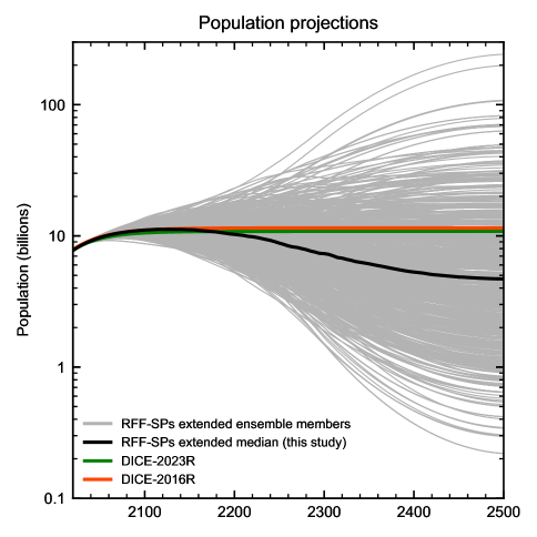
Figure 1: Population projections from the 10,000 RFF-SPs from 2020 to 2300, extended to 2500 using the average growth rate of the last fifty years, declining to zero growth over 2300–2500 (coloured lines). The thick black line is the ensemble median, used for the population projection in this study.

1.3 Model for future land-use CO₂ emissions

The DICE-2016R and DICE-2023R models use exogenous time series of CO₂ emissions from agriculture, forestry and other land use (AFOLU). These emissions do not result from fossil fuel combustion and have differing economic and social drivers to fossil fuel emissions that are not modelled explicitly in DICE. Nevertheless, the AFOLU sector will play a vital role in climate change mitigation, and land-based carbon dioxide removal strategies (afforestation and reforestation) are featured heavily in process-based (PB-) IAM scenarios that limit global mean temperatures to 1.5°C or 2°C [6]. Therefore, it could be reasonably expected that a mitigation scenario that took strong action on fossil emissions would also address the AFOLU sector, even if the causal drivers are not strongly linked.

In this regard, we seek a regression relationship predicting CO₂ AFOLU emissions $E_{\mathrm{AFOLU}}$ from FFI emissions $E_{\mathrm{FFI}}$ and period $t$, derived from 1202 PB-IAM scenarios from the IPCC WG3 database from 2030 to 2100 [7]:

$$E_{\mathrm{AFOLU}}=\alpha+\beta_{1}E_{\mathrm{FFI}}+\beta_{2}t.$$ (1)

Figure 2(a) shows there is a positive, time-dependent relationship between fossil emissions and AFOLU emissions from PB-IAM scenarios justifying the form of eq. 1 ($r^{2}=.47$). We derive $\alpha=1.54$ GtCO₂ yr^-1, $\beta_{1}=0.0464$, $\beta_{2}=-0.189$ GtCO₂ yr^-1 period^-1. Equation 1 is only defined to 2100. To extend to 2500, we follow the assumption of a phase down to zero CO₂ AFOLU emissions by 2150 used for the SSP scenario extensions in [8]. This is achieved by multiplying eq. 1 by a logistic curve $l(t)$ centred around $t=35$ (model year 2125):

$$l(t)=\left(1-\frac{1}{1+e^{-(t-35)}}\right).$$ (2)

The comparison of our ensembles to the exogenous CO₂ AFOLU emissions in DICE-2016R and DICE-2023R is shown in fig. 2(b). All of our scenarios have negative AFOLU emissions during the later 21st century, which is typical of PB-IAM scenarios (fig. 2(a)). This is in contrast to the DICE time series where AFOLU emissions converge to zero from above. The impact of the logistic phase out can be seen in the 2100–2150 period. Our year-2023 CO₂ AFOLU emissions value, derived solely from the regression relationship, is also slightly closer to the historical best estimate from the Global Carbon Project (GCP; black line near the left axis in fig. 2(b)) than in DICE-2023, though it should be cautioned that the 2022 land use emissions from GCP is preliminary, and land use emissions have large uncertainty.

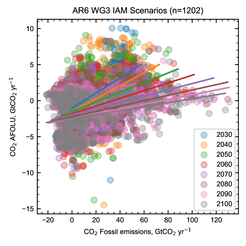
(a) Comparison of $E_{\textrm{AFOLU}}$ with $E_{\textrm{FFI}}$ for 1202 PB-IAM scenarios submitted to the IPCC AR6 WG3 database. Regression lines drawn at 10 year intervals from 2030 to 2100.

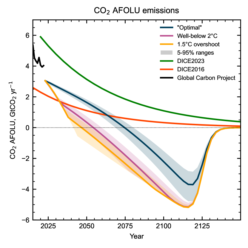
(b) Comparison of $E_{\textrm{AFOLU}}$ from the three scenario ensembles in this study (coloured lines and uncertainty ranges) with DICE-2016 (dotted) and DICE-2023 (dashed) exogenously supplied time series. Historical best estimate emissions from Global Carbon Project are shown in black as a comparison.

Figure 2: AFOLU emissions derivation for the scenario pathways in this study.

2 Reduced version of FaIR v2.1.0 in DICE

The Finite-amplitude Impulse Response (FaIR) model is a reduced-complexity climate model used to project global mean surface temperatures from emissions of greenhouse gases and short-lived climate forcers, and other anthropogenic and natural influences on the climate system [9, 10, 11]. We implement a reduced version of FaIR in DICE for future projections (2023–2500) that is based on FaIR v2.1.0. A model description paper for FaIR v2.1.0 is not yet in the scientific literature but it is similar to v2.0.0 [9]. The specific implementation for DICE is described below.

DICE calculates CO₂ emissions from fossil fuel and industry $E_{\mathrm{FFI}}$ from economic activity, abatement level and energy intensity (eq. 2, main manuscript). Our treatment of CO₂ emissions from agriculture, forestry and other land use (AFOLU) are described in section 1.3. FaIR-DICE, based on DICE-2016R, does not model any other anthropogenic greenhouse gas or short-lived climate forcer explicitly. Therefore our reduced version of FaIR is limited to the carbon cycle module and the temperature response module (both described below) with non-CO₂ forcing introduced exogenously (described in the next section).

2.1 Carbon cycle model

We retain the four time-constant model of atmospheric CO₂ decay to a pulse emission from FaIR v2.0.0. Written in forward difference mode, this is

$$R_{i}(t+1)=a_{i}E_{\textrm{FFI}}(t)\alpha(t)\tau_{i}\left(1-\exp\left(-\frac{\Delta t}{\alpha\tau_{i}}\right)\right)+R_{i}(t)\exp\left(-\frac{\Delta t}{\alpha\tau_{i}}\right)$$ (3)

where $R_{i}$ is the carbon content in pool $i$, $\Delta t$ is the model timestep (3 yr), $a_{i}$ is the amount of fresh emissions allocated to each pool, $\tau_{i}$ is the e-folding lifetime of each pool, and $\alpha$ is the lifetime scaling factor that models the effect of carbon cycle feedbacks. The values of $a_{i}$ and $\tau_{i}$ are derived from Earth System and intermediate complexity models in [12] (table 1). In FaIR v2.1.0 a user-definable $\Delta t$ is incorporated, partly for applications including IAM coupling. Previously, the model timestep was hard-coded to be one year.

Table 1: Partition fractions and lifetimes of the four carbon box impulse-response model in FaIR

Pool $i$	Partition fraction $a_{i}$	Lifetime $\tau_{i}$ (yr)
1	0.2173	$10^{9}$ (essentially $\infty$)
2	0.2240	394.4
3	0.2824	36.54
4	0.2763	4.304

Carbon uptake efficiency reduces with increasing warming and accumulated CO₂ in land and ocean sinks [13, 14]. In FaIR, the increase in atmospheric lifetime of CO₂ is parameterised by $\alpha$. $\alpha$ is determined from the 100-year time-integrated airborne fraction from a pulse of CO₂ emissions, $I_{100}$:

$$\alpha(t)=g_{0}\exp\left(\frac{I_{100}(t)}{g_{1}}\right)$$ (4)

where the airborne fraction is the proportion of CO₂ remaining in the atmosphere following a pulse emission, and follows the empirically derived equation [11]

$$I_{100}(t)=r_{0}+r_{u}(1-f_{a}(t))G(t)+r_{t}T_{1}(t)+r_{a}f_{a}(t)G(t).$$ (5)

In eq. 5, $r_{0}$ is the pre-industrial value of $I_{100}$, $r_{u}$ is the sensitivity of $I_{100}$ to accumulated carbon in land and ocean sinks, $r_{t}$ is sensitivity of $I_{100}$ to global mean surface temperature anomaly $T_{1}$, and $r_{a}$ is the sensitivity of $I_{100}$ to airborne CO₂. $G$ represents cumulative CO₂ emissions since pre-industrial and $f_{a}$ is the airborne fraction of CO₂ since pre-industrial (total increase of CO₂ in the atmosphere divided by $G$). $I_{100}$ has units of yr.

In eq. 4, $g_{0}$ and $g_{1}$ are normalisation constants defined as

$$g_{1}=\sum_{i}a_{i}\tau_{i}\left(1-\left(1+\frac{H}{\tau_{i}}\right)\exp\left(-\frac{H}{\tau_{i}}\right)\right)$$ (6)

$$g_{0}=\exp\left(-\frac{\sum_{i}a_{i}\tau_{i}\left(1-\exp\left(-\frac{H}{\tau_{i}}\right)\right)}{g_{1}}\right)$$ (7)

with $H=100$ yr. The atmospheric CO₂ concentration $C_{\mathrm{CO}_{2}}$ is the sum of the four boxes added to the pre-industrial CO₂ atmospheric concentration ($C_{\mathrm{CO}_{2},\mathrm{ref}}$), i.e.

$$C_{\mathrm{CO}_{2}}(t)=C_{\mathrm{CO}_{2},\mathrm{ref}}+\sum_{i}R_{i}(t).$$ (8)

2.2 Effective radiative forcing

The total effective radiative forcing (ERF) $F$ is given by

$$F(t)=F_{\mathrm{CO}_{2}}(t)+F_{\mathrm{ext}}(t)$$ (9)

where $F_{\mathrm{CO}_{2}}$ is the CO₂ component and $F_{\mathrm{ext}}$ is the and the exogenous non-CO₂ component. In this reduced version, the CO₂ forcing is computed from concentrations as [15]

$$F_{\mathrm{CO}_{2}}(t)=F_{2\times\mathrm{CO}_{2}}\frac{\log(C_{\mathrm{CO}_{2}}(t)/C_{\mathrm{CO}_{2},\mathrm{ref}})}{\log 2}.$$ (10)

In eq. 10, $F_{2\times\mathrm{CO}_{2}}$ is the effective radiative forcing from a doubling of CO₂ above pre-industrial concentrations with a best estimate value of 3.93 W m^-2 [16]. More complex relationships exist for CO₂ forcing that incorporate band overlaps between different greenhouse gases [17, 8], however, as concentrations of other gases are not book-kept in DICE, the simpler formula in eq. 10 is used in FaIR-DICE.

2.3 Temperature response module

For computing the temperature response to effective radiative forcing, FaIR uses an impulse-response formulation of the well-known $n$-layer energy balance model [18]. The implementation here very closely follows the model of Cummins et al. [19]. FaIR v2.1.0 allows for autocorrelated stochastic internal variability in temperature and forcing following [19], but we do not use this in the present study. There is evidence that inclusion of internal variability increases the social cost of carbon (SCC) [20] and this would be a valuable additional study in this setup.

We use $n=3$ layers, expected to be sufficient to capture short- and long-term climate responses to forcing [9, 19]. The impulse-response model in forward timestepping mode can be written as

$$\mathbf{T}(t+1)=\mathbf{A_{d}T}(t)+\mathbf{b_{d}}F(t)$$ (11)

where $\mathbf{T}=[T_{1}(t),T_{2}(t),T_{3}(t)]$ is a column vector of temperature anomalies representing the near-surface ocean layer and atmosphere, middle ocean, and deep ocean respectively. $T_{1}$ is used as global mean surface temperature anomaly throughout this study.

$\mathbf{A_{d}}$ and $\mathbf{b_{d}}$ are computed using the discretisation method of Cummins et al. [19] with one modification in that we discard the first column and top row of $\mathbf{A_{d}}$ and first entry of $\mathbf{b_{d}}$ as calculated in [19], as we do not use stochastic variability in forcing or temperature. The reader is referred to sections 4a and 4b of Cummins et al. [19] for the calculation. The Cummins et al. method takes a matrix of energy balance model parameters $\mathbf{A}$ where

$$\mathbf{A}=\frac{1}{\Delta t}\begin{bmatrix}-\gamma\Delta t&0&0&0\\ 1/C_{1}&-(\kappa_{1}+\kappa_{2})/C_{1}&\kappa_{2}/C_{1}&0\\ 0&\kappa_{2}/C_{2}&-(\kappa_{2}+\epsilon\kappa_{3})/C_{2}&\epsilon\kappa_{3}/C_{2}\\ 0&0&\kappa_{3}/C_{3}&-\kappa_{3}/C_{3}\end{bmatrix}$$ (12)

and a column vector $\mathbf{b}=[\gamma,0,0,0]$ as inputs. Here, $\kappa_{j}$ [W m^-2 K^-1] are heat transfer coefficients between adjacent ocean layers (with $-\kappa_{1}$ equivalent to the climate feedback parameter more commonly denoted as $\lambda$ in climate science literature), $C_{j}$ are heat capacities of each ocean layer [W m^-2 yr K^-1], and $\epsilon$ is the deep ocean efficacy parameter incorporated to simulate a forced pattern effect present in many Earth system models [21, 22]. $\gamma$ is a parameter describing autocorrelation in the radiative forcing time series but is redundant if internal variability is not used. These parameters are easily calibrated to Earth System models (ESMs) as demonstrated in [18, 19].

3 Constrained probabilistic ensemble of FaIR v2.1.0

A semi-automated software package fair-calibrate exists for producing calibrated, constrained probabilistic ensembles from the FaIR model (starting from FaIR v2.1.0). A separate manuscript is in preparation describing this process in detail. We provide an overview relevant to results in this paper here. We use the procedure and parameter values from v1.0.2 of fair-calibrate which is available from [23]. This reference also contains the calibration code which is fully reproducible. The calibration procedure produced uses the full standalone (rather than reduced, DICE-coupled) FaIR v2.1.0 model, is run at a one-year rather than three-year time step, and has internal variability switched on.

3.1 Calibration

3.1.1 Climate response

The parameters of the three-layer energy balance model ($\kappa_{j}$, $C_{j}$, $\epsilon$ and $\gamma$, along with the ERF from a quadrupling of CO₂, $F_{4\times\mathrm{CO}_{2}}$) are calibrated to the response of 49 abrupt-4xCO2 ESMs participating in the Coupled Model Intercomparison Project Phase 6 (CMIP6) using the maximum likelihood method of Cummins et al. [19]. We use the first 150 years from the quadrupled CO₂ run for consistency, even for models where more years are available. This provides us with a set of nine climate response parameters from 49 ESMs.

3.1.2 Carbon cycle feedbacks

The parameters dictating the carbon cycle feedbacks are $r_{0}$, $r_{u}$, $r_{t}$ and $r_{a}$ defined in eq. 5. The parameters are calibrated from 11 carbon-cycle enabled Earth System models from CMIP6 using 1pctCO2 and 1pctCO2-rad experiments as described in [9].

3.1.3 Non-CO₂ forcing

The full FaIR model that is used for the historical spin up also uses CMIP6 model results to calibrate the effective radiative forcing from aerosol-cloud interactions (ERFaci) to emissions of precursor species in 11 CMIP6 models (a similar method to [24]), the sensitivities of chemically active species to ozone formation and destruction in six CMIP6 models (from [25]), and the sensitivities of chemically active species to methane lifetime in four CMIP6 models (from [26, 27]). There are many more anthropogenic and natural components that influence non-CO₂ forcings, with these sensitivities based on assessments from the IPCC Sixth Assessment Report (AR6) rather than CMIP6 models [16, 28].

3.2 Sampling

We use a prior ensemble size of 1,500,000 parameter sets based on CMIP6 model calibrations or AR6 distributions, and use these parameter sets to run the full version of FaIR offline (i.e. uncoupled to DICE) from 1750–2100 under the historical + SSP2-4.5 scenario. Emissions of 53 greenhouse gas and short-lived climate forcers under historical + SSP2-4.5 are provided by the Reduced Complexity Model Intercomparison Project (RCMIP), with data available from [29]. For short-lived climate forcers (SO₂, BC, OC, NH₃, CO, NMVOC, NOx), RCMIP uses the same input emissions sources prepared for running CMIP6 models, whereas greenhouse gases emissions are based on respected emissions inventories for CH₄ and N₂O and estimated from inversions of concentrations for halogenated greenhouse gases. We do not use the CO₂ FFI and CO₂ AFOLU emissions from RCMIP for the historical period up to 2021, instead using data from Global Carbon Project [30] which is more up-to-date and ensures the beginning of the DICE projection period uses a more recent estimate of CO₂ emissions. To transition to the SSP2-4.5 scenario, the future emissions are harmonized [31] to the updated GCP historical to ensure a smooth transition from the updated baseline to the future scenario.

3.2.1 Climate response

The nine energy balance model parameters are sampled from a multi-dimensional kernel density estimate function that is generated from the 49 CMIP6 models used in the calibration.

3.2.2 Aerosol-cloud interactions

There are four parameters that are used to model the ERFaci in FaIR, which are the sensitivity to SO₂, BC, and OC emissions, and a scale factor. The shape parameters are sampled from correlated kernel density estimates that are constructed by the fits to 11 CMIP6 models. The scale parameter is selected such that the resulting ERFaci in each ensemble member for the 2005–2014 period relative to 1750 is uniform in the range $-2$ to 0 W m^-2.

3.2.3 Aerosol-radiation interactions

A number of species are involved in contributing to the ERF from aerosol-radiation interactions (ERFari) [32]. Aerosol formation is dominated by sulfate (primary source SO₂ emissions), BC, OC and nitrate (dominant source NH₃ emissions), with minor contributions from NOx, NMVOC, CH₄, N₂O, and halogenated greenhouse gases.

A forcing efficiency for each species is calculated by dividing its contribution to ERFari as assessed by IPCC AR6 [32] by its change in emissions (or concentrations for greenhouse gases) between 1750 and 2019. The headline assessment of ERFari is $-0.3$ W m^-2 from 1750 to 2005–2014, which is reproduced using these forcing efficiencies (the assessed ERFari in 2019 was $-0.22$ W m^-2 owing to reductions in emissions). To sample uncertainties, we use a uniform distribution for the forcing efficiency of each species that ranges from zero to a factor of two times the best estimate. The addition of nine uniform random variables leads to an overall prior distribution of ERFari that is approximately trapezoidal.

3.2.4 Carbon cycle feedbacks

The carbon cycle feedback strengths are dictated by the $r_{0}$, $r_{u}$, $r_{t}$ and $r_{a}$ parameters in eq. 5. A four-dimensional kernel density estimate using the 11 model CMIP6 model calibrations in [9] (their table 3) were used to sample from.

3.2.5 Ozone forcing

The starting point for sampling ozone forcing is the IPCC AR6 assessment of total (tropospheric plus stratospheric) ozone forcing from 1750 to 2019 of +0.47 W m^-2. This is based on the six-model mean historical time series from CMIP6 models in [25]. A correction for historical warming is applied to this time series using CMIP6 data of $-0.037$ W m^-2 K^-1 [27] which is backed out of the forcing time series; this is because warming produces more water vapour, which produces more OH radicals, which are a chemical sink for ozone. Ozone is produced from chemical reactions that are facilitated from CH₄, NOx, N₂O, NMVOC and CO, and destroyed by halogenated greenhouse gases. The contribution of each factor to total ozone (in W m^-2) is derived from six CMIP6 models in [26] for the 1850–2014 period which is then scaled up for each species to match the overall 1750–2019 assessment from AR6. The uncertainty in the ozone forcing contribution from each specie is also taken from [26] and scaled. These values are converted to a forcing efficiency for each specie, as is done for ERFari. A Gaussian distribution is assumed for the forcing efficiency of each parameter.

3.2.6 Effective radiative forcing uncertainty

IPCC AR6 considered the effective radiative forcing in a few aggregated categories, and provided uncertainty ranges for each [16] (see table 2). For many categories we used the same uncertainty ranges as AR6, which are applied as a scaling factor to the historical and future forcing time series (table 2). For solar forcing, the amplitude of the solar variability around a mean value is scaled by a factor, and an underlying trend over 1750 to 2019 is added. For ozone and aerosols, we do not use the AR6 uncertainties as priors but the priors described in the various preceding sections, which are similar to or wider than the corresponding AR6 assessments.

3.2.7 CO₂ initial concentrations

The pre-industrial concentrations of many greenhouse gases are uncertain. As we use present-day CO₂ concentrations as a constraint, we consider the possibility that the atmospheric concentration of CO₂ in 1750 was slightly higher or lower than the IPCC’s best estimate. Clearly, as we do not have in-situ observations from this time, the uncertainty in concentrations is greater than in the present day. We use the AR6 assessment, drawing samples from a Gaussian distribution with mean 278.3 ppm and 90% range 2.9 ppm [33]. Variation in pre-industrial CO₂ values affects both the carbon cycle and the CO₂ forcing calculation (eq. 10).

Table 2: Effective radiative forcing scaling factor distributions used in the prior parameter sampling for FaIR. Symmetric uncertainty ranges are Gaussian, asymmetric ranges are half-Gaussian where two separate distributions are used for values below and above the best estimate. The solar forcing trend is Gaussian around +0.01 W m^-2. Some forcers do not take their uncertainties from AR6 and use different prior distribution uncertainties given by the corresponding section number.

Forcer	90% uncertainty around best estimate, or source
CO2	$\pm 12\%$
CH4	$\pm 20\%$
N2O	$\pm 14\%$
Halogenated GHGs	$\pm 19\%$
Stratospheric water vapour	$\pm 100\%$
Ozone	section 3.2.5
Aerosol-radiation interactions	section 3.2.3
Aerosol-cloud interactions	section 3.2.2
Aviation contrails	$-66\%$ to $+70\%$
Black carbon on snow	$-100\%$ to $+125\%$
Land use and irrigation	$\pm 50\%$
Solar forcing amplitude	$\pm 50\%$
Solar forcing trend 1750–2019	$-0.06$ to $+0.08$ W m-2 (Gaussian)
Volcanic forcing	$\pm 25\%$

3.3 Constraining

From the 1,500,000 member prior ensemble we seek to produce a smaller constrained ensemble of parameters that fit both observational constraints and IPCC assessments. The prior ensemble produces a very wide range of climate projections, most of which are implausible and not useful for using for future projections (fig. 3(a)).

3.3.1 First step: root-mean-square comparison to historical warming

The first constraining step uses a root-mean-square error (RMSE) comparison between the time series of historical temperature observations from the IPCC assessment [33] and each FaIR ensemble member. Ensemble members that differ from the historical time series with a RMSE of more than 0.16 K are rejected. This rules out 92% of the original ensemble, and produces projections that are much closer to historical observations (fig. 3(b)).

3.3.2 Second step: Distribution fitting

The second constraining step takes the ensemble members that pass the RMSE test and attempts to simultaneously fill distributions of observations and climate system metrics that were assessed in the IPCC AR6 WG1 [28]. The distributions are given in table 3. A three-parameter skew-normal distribution is used to fit a distribution to the percentiles given in table 3 (“Target” column), which reduces to a Gaussian where the upper and lower ranges are symmetric around the best estimate. Distribution fitting further narrows the range of climate projections (fig. 3(c)), particularly for future warming.

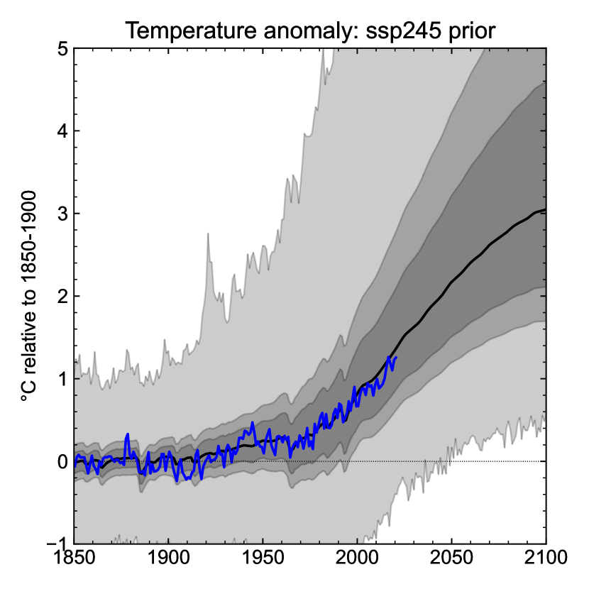
(a) Prior

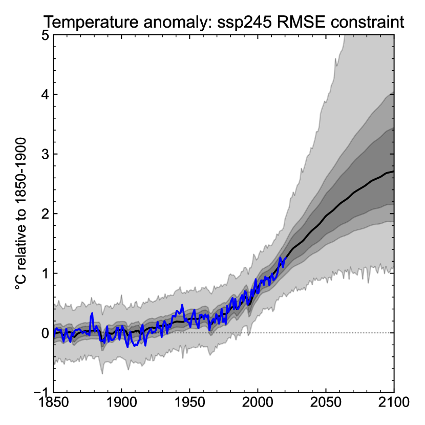
(b) After RMSE constraint

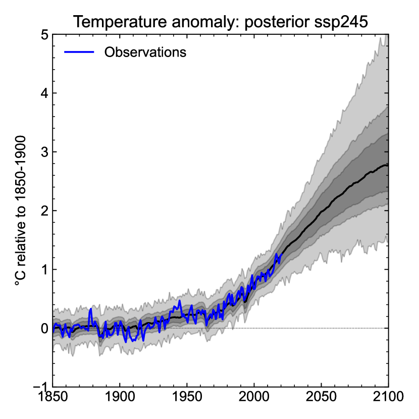
(c) Final reweighed ensemble

Figure 3: SSP2-4.5 emissions run in FaIR for the prior, RMSE-only constraint and final, reweighted ensemble. In each subplot, the full minimum to maximum range is in light grey, the 5-95% range mid-grey, 16-84% range dark grey and ensemble median black. Historical temperature observations are shown in blue.

The size of the final reweighted posterior is user-definable, but is limited by the number of runs passing the RMSE step, which itself depends on the size of the prior. We choose 1001 ensemble members for the final ensemble. This number is sufficiently large to fill the uncertainty space (consistent with constraints) and small enough to be computationally lightweight in the FaIR-DICE coupled system. Typically, ensemble sizes of a few hundred or a few thousand are used in reduced-complexity climate model applications [34]. The final 1001-member constrained, reweighted posterior distribution is, in most cases, close to the target (table 3 “Ensemble” column).

Table 3: Target distributions, and percentiles from the reweighted constrained posterior, for climate system assessments used to constrain FaIR. All distributions are from the IPCC AR6 Working Group 1.

	Target			Ensemble
Variable	5%	50%	95%	5%	50%	95%
ECS [K]	2.0	3.0	5.0	1.97	3.04	5.20
TCR [K]	1.2	1.8	2.4	1.34	1.84	2.48
Historical warming 1850–1900 to 1995–2014 [K]	0.67	0.85	0.98	0.71	0.85	0.99
ERFari 1750 to 2005–2014 [W m-2]	$-0.6$	$-0.3$	0.0	$-0.60$	$-0.30$	+0.02
ERFaci 1750 to 2005–2014 [W m-2]	$-1.7$	$-1.0$	$-0.3$	$-1.75$	$-1.04$	$-0.34$
Total aerosol forcing 1750 to 2005–2014 [W m-2]	$-2.0$	$-1.3$	$-0.6$	$-2.06$	$-1.37$	$-0.59$
CO2 concentration in 2014 [ppm]	396.95	397.55	398.15	396.87	397.56	398.24
Ocean heat content change 1971 to 2018 [ZJ]	286	396	506	275	401	514
SSP2-4.5 warming 1995–2014 to 2081–2100 [K]	1.24	1.81	2.59	1.22	1.83	2.70

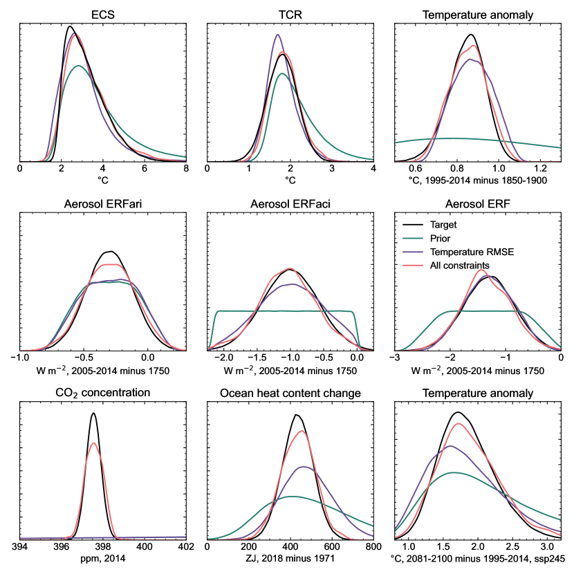
Figure 4: Constraining the FaIR posterior to nine IPCC assessments of observable and emergent climate metrics. In each distribution, the green curve shows the prior distribution derived from a 1,500,000 member ensemble in section 3.2. The purple curves shows the distributions after the RMSE filtering step (section 3.3.1). The red curves show the final reweighted posterior distributions (section 3.3.2). The aim is to match the red curves as closely as possible to the target distributions, constructed from table 3, in black curves.

The distribution matching procedure to produce a constrained ensemble used here is similar and updated from that that was developed as part of the IPCC’s Sixth Assessment Report (AR6) WG1, supported by the Reduced Complexity Model Intercomparison Project (RCMIP) [35, 34, 16, 28]. This evaluated the ability of simple climate models to reproduce historically observed climate change and expert assessments of emergent climate variables. Models that were fit for purpose were carried forward to provide climate projections from PB-IAM emissions scenarios for the IPCC AR6 WG3 report [36, 37]. FaIR v1.6.2 was one simple climate model that was deemed to be fit for purpose [16]. It was not the only one, but of the three that passed the test it is (a) structurally simple and (b) open source (at time of AR6 publication), lending it to be easily used inside the optimization code of a CB-IAM [38, 39].

4 Historical spin-up and non-CO₂ forcing

In the reduced version of FaIR in DICE, the carbon pools $R_{i}$, temperatures in each energy balance model layer $T_{j}$ and non-CO₂ effective radiative forcing $F_{\mathrm{ext}}$ need initial values to start from in 2023. Furthermore, $F_{\mathrm{ext}}(t)$ must be provided as an exogenous time series in each ensemble member for 2023–2500.

To do this, we run the 1001-member final calibrated, constrained ensemble from section 3.3.2 in FaIR, with all forcings (but no internal variability) and uncoupled to DICE, for 1750 to 2500 in 3-year time steps. We run the SSP1-1.9, SSP1-2.6 and SSP2-4.5 emissions scenarios, which provide the non-CO₂ forcing time series for the 1.5°C overshoot, well-below 2°C and “optimal” scenarios that we run in DICE. These non-CO₂ forcing time series are saved out for 2023 to 2500 for each ensemble member and scenario. The values of $T_{j}$ and $R_{i}$ are saved out for 2023 for each ensemble member and scenario, and used as initial conditions.

As described in section 2.2 in the main paper the historical all-forcing implementation of FaIR uses a different relationship for calculating ERF from CO₂ than the CO₂-only DICE-coupled implementation. We also save out the value of $F_{2\times\mathrm{CO}_{2}}$ used in the computation of future CO₂ forcing in FaIR-DICE (eq. 10).

5 Climate uncertainty is not just ECS

Consideration of climate uncertainty in CB-IAM analyses may be limited to cases where the eqilibrium climate sensitivity (ECS) is varied but other climate system parameters are held at their best estimate or default values [40, 41, 42, 43]. Notably, there is a strong anti-correlation between ECS and aerosol radiative forcing in historically-consistent climate simulations [10, 44]. A high ECS could also be masked by a slow response timescale of the deep ocean or a sea-surface-temperature mediated pattern effect [45].

We briefly demonstrate why full climate uncertainty needs to be taken into account, and varying the ECS alone is not sufficient. In fig. 5, we run FaIR over the historical period (1750–2023, at three year time steps) with median parameter values from the 1001-member calibrated, constrained FaIR ensemble, except for the climate feedback parameter $-\kappa_{1}$ which is inversely proportional to ECS. We choose $-\kappa_{1}$ to produce ECS=2°C, 3°C and 5°C (5th, 50th and 95th percentiles of the IPCC AR6 distribution). While ECS=3°C (by design) reproduces historical temperatures well, ECS=2°C is too cool, and ECS=5°C is too warm (substantially so). Different parameter combinations would permit historically consistent climates with ECS=2°C (or lower) and ECS=5°C (or higher) but with very different future warming outcomes. Therefore, varying only ECS and not the full spectrum of climate uncertainty can result in historically inconsistent climates which reduces confidence in projections made using climate-economic models.

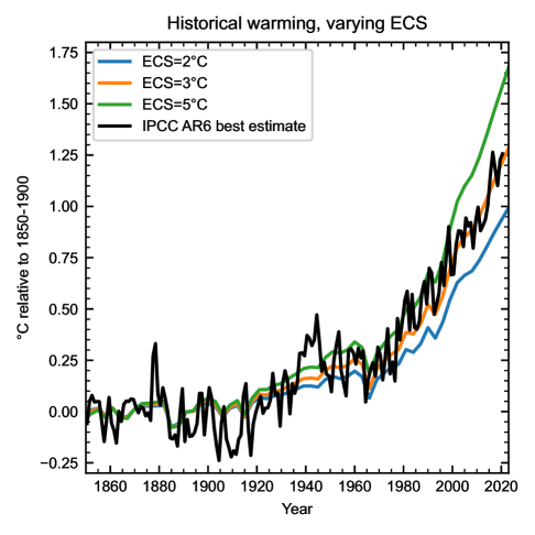
Figure 5: Historical climate projected with FaIR with the climate feedback parameter varied to produce ECS=2°C, 3°C and 5°C and all other climate parameters at their ensemble median values from the 1001-member calibrated and constrained ensemble. Observed global mean surface temperature in black.

6 Comparison of results with DICE-2023 and DICE-2016

We now turn to the beta version of DICE-2023R which incorporates the climate and carbon cycle modules from FaIR v1.0 [3]. Alongside the climate module update, DICE-2023R includes more recent updates to the economic and population assumptions over DICE-2016R (as does our version), but the economic part of the IAM is structrually unchanged. For completeness, we also compare our results to DICE-2016R. We compare “optimal” scenarios across the three versions of DICE. DICE-2023R and DICE-2016R both produced 2°C and 1.5°C style scenarios but under different definitions to ours and the comparisons are less meaningful. The GAMS code for DICE-2023R and DICE-2016R was obtained from the online appendix to [3] (accessed 16 June 2023), and included as part of the software repository that accompanies this paper.

The comparison of the three models’ “optimal” scenarios is shown in fig. 6. The improvement in carbon cycle dynamics between DICE-2016R (orange) and DICE-2023R (green) is evident in the trajectory of atmospheric CO₂ concentrations (fig. 6b) over the next 100 years. The DICE-2016R concentrations are substantially higher than both our FaIR-DICE (blue) and DICE-2023R despite lower total CO₂ emissions (fig. 6a). Nevertheless, the carbon cycle parameterisation in DICE-2023 is more sensitive than in our study given higher CO₂ concentrations over the next 100 years despite lower emissions before 2100. As our CO₂ concentrations in the present-day are specifically constrained for in the posterior ensemble (main paper fig. 1b; supplement fig. 4) and the carbon cycle models in FaIR-DICE and DICE-2023R are similar, the differences are likely due to a slightly outdated set of carbon cycle parameters used in DICE-2023R.

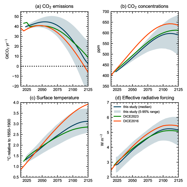
Figure 6: Climate projections under the “optimal” scenario for the FaIR-DICE implementation used in this study (blue lines ensemble medians; shaded regions 5–95% ranges) compared to DICE-2023R (green) and DICE-2016R (orange).

Temperature (fig. 6c) responds to effective radiative forcing (fig. 6d). The ERF is similar between the three versions, particularly our version compared to DICE-2023R. This leads to fairly similar temperature projections until 2075, at which point DICE-2023R warms slower than our version. DICE-2023R uses a two-layer impulse response model for climate which is similar to our three-layer model, and has the same ECS and TCR as our ensemble median. The differences may arise from the timescales of climate response; DICE-2023R uses FaIR v1.0 default values which are a CMIP5 multi-model mean, whereas we use a constrained probabilistic set drawn from CMIP6 model priors. The temperature response in DICE-2023R is clearly a large improvement over DICE-2016R and well within our uncertainty range.

In summary, DICE-2023R is capturing many of the key behaviours of our version of FaIR-DICE and could be improved further with a re-calibration of the carbon cycle and possibly the climate response. The models differ in other ways including their population and economic assumptions, time step, time horizon, and the fact that DICE-2023R considers non-CO₂ greenhouse gases as a separate forcing category. A full comparison of the two models is beyond the scope of this study.

7 Comparison to Rennert et al. (2022)

One additional case we run is attempting to recreate the National Academies of Science, Engineering and Medicine (NASEM) update to the SCC from Rennert et al. [4]. We do this in order to attempt to benchmark our results with a more commonly used discount rate of 2%.

Rennert et al. use a different method to calculate SCC, where 10,000 projections of population (which we adopt, fig. 1) and emissions of CO₂, CH₄ and N₂O are generated following expert elicitation, and SCC is calculated as the marginal discounted damages from an additional pulse of CO₂ into the future. They also use a different integrated assessment model (GIVE) and a different climate damage function to calculate SCC. Climate uncertainty is considered in the overall system and is provided by the IPCC AR6 calibration of FaIR v1.6.2 [10, 28].

The discount rate $r$, equivalent to a risk-free interest rate, is given by the Ramsey equation

$$r=\rho+\eta g$$ (13)

where $\rho$ is the pure rate of time preference, $\eta$ is the marginal utility of consumption and $g$ is the per-capita annual growth in consumption [46]. In order to achieve a near-term discount rate of 2%, Rennert et al. calibrated the $\rho$ and $\eta$ parameters to fit future expected evolution in interest rates from the economic literature that matched the desired value of $r$ in the near term. They obtain $\rho=0.2\%$, $\eta=1.24$, implying $g=1.45\%$.

We re-run our 1001 member ensemble of FaIR-DICE using $\rho=0.2\%$, $\eta=1.24$, retaining SSP2-4.5 as the non-CO₂ time series and include this scenario as an additional projection in fig. 7. We find this leads us to a median near-term discount rate of 2.5% and a median SCC of $84 (t CO₂)^-1 (table 4). Using the NASEM discount parameters leads to an SCC that is less than half of that reported for the 2% discount case of $185 (t CO₂)^-1 in [4]. Rennert et al. also show results from a 2.5% discount rate, where SCC is $118 (t CO₂)^-1, 40% higher than our value with the same discount rate.

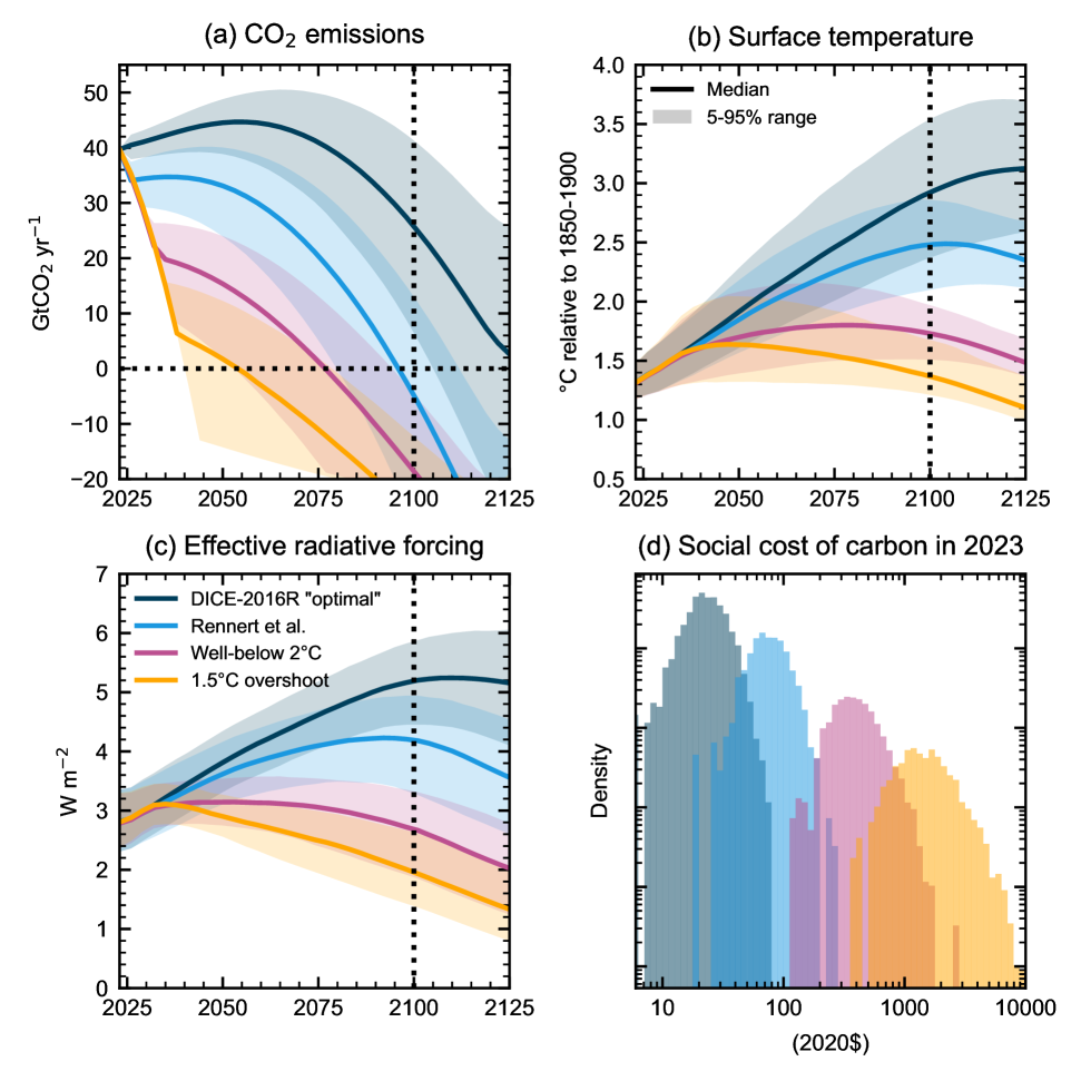
Figure 7: Emissions, climate and economic projections for four scenarios using FaIR-DICE, with the additional scenario included that uses the discount parameters from Rennert et al.. (a) CO₂ emissions from energy and industrial processes for the “optimal” (dark blue), Rennert et al. (light blue), 2°C (pink) and 1.5°C (yellow) scenarios. (b) Temperature projections. (c) Total effective radiative forcing projections. (d) Histogram of year-2023 SCC (in 2020$) on a log-log scale. In (a-c), light shading shows 5-95% range and solid lines show ensemble medians.

Table 4: Key results from the four scenarios including our implementation of the Rennert et al. discounting parameters. All correlations are significant at the 1% level.

Variable	“optimal”	Rennert et al.	Well below 2°C	1.5°C overshoot
CO2 emissions 2050 (Gt CO2 yr-1)	45 (39–49)	33 (24–40)	15 (2–24)	2 (−14 to +12)
CO2 emissions 2100 (Gt CO2 yr-1)	25 (5–41)	−6 (−21 to +12)	−19 (−23 to −5)	−23 (−23 to −13)
Net zero CO2 year	2129 (2105–2152)	2096 (2080–2112)	2077 (2053–2094)	2054 (2040–2079)
Social cost of carbon 2023 (2020$ (t CO2)-1)	26 (15–44)	84 (49–142)	439 (237–934)	1759 (821–4434)
Peak warming (°C relative to 1850–1900)	3.1 (2.7–3.7)	2.5 (2.1–2.9)	1.8 (1.5–2.2)	1.6 (1.3–2.1)
Warming 2100 (°C relative to 1850–1900)	2.9 (2.4–3.6)	2.5 (2.1–2.9)	1.7 (1.5–2.0)	1.4 (1.2–1.7)
Effective radiative forcing 2100 (W m-2)	5.2 (4.4–5.9)	4.2 (3.3–4.9)	2.7 (1.9–3.3)	1.9 (1.4–2.6)
ECS/SCC correlation coefficient	.51	.66	.74	.74
ECS/2050 CO2 emissions correlation coefficient	−.48	−.61	−.72	−.76
2014 aerosol forcing/SCC correlation coefficient	−.64	−.63	−.60	−.59
2014 aerosol forcing/2050 CO2 emissions correlation coefficient	.61	.61	.59	.56
Near-term discount rate (%)	3.1 (3.1–3.2)	2.5 (2.4–2.6)	1.4 (1.2–1.6)	0.6 (0.2–0.8)

The higher $r$ value that we obtain with the same discounting parameters implies a higher near-term growth rate in our model compared to [4]. Indeed, our first to second period per capita growth is 1.84% per year.

DICE and GIVE are different integrated assessment models, and should not necessarily be expected to give the same results even if the climate system components are the same in both models (which they are not). Rennert et al. in their Table 1 show that switching from DICE to GIVE, and then updating the damage function from DICE-2016R to theirs increases the SCC by 80%. Therefore, it is expected that our SCC estimate would be lower than that provided in [4] for a 2.5% discount rate. It should also be noted that achieving an ensemble median 2% discount rate in DICE would require an iterative approach to adjusting the $\rho$ and $\eta$ parameters, as unlike in GIVE, per-capita growth rates in DICE are dynamic and solved as part of the overall system.

References

- Nordhaus and Sztorc [2013] William Nordhaus and Paul Sztorc. DICE 2013R: Introduction and user’s manual. Yale University and the National Bureau of Economic Research, USA, 2013.
- Nordhaus [2017] William D. Nordhaus. Revisiting the social cost of carbon. Proceedings of the National Academy of Sciences, 114(7):1518–1523, 2017. doi: 10.1073/pnas.1609244114.
- Barrage and Nordhaus [2023] Lint Barrage and William D. Nordhaus. Policies, projections, and the social cost of carbon: Results from the dice-2023 model. Working Paper 31112, National Bureau of Economic Research, April 2023. URL http://www.nber.org/papers/w31112.
- Rennert et al. [2022] Kevin Rennert, Frank Errickson, Brian C. Prest, Lisa Rennels, Richard G Newell, William Pizer, Cora Kingdon, Jordan Wingenroth, Roger Cooke, Bryan Parthum, David Smith, Kevin Cromar, Delavane Diaz, Frances C. Moore, Ulrich K. Müller, Richard J. Plevin, Adrian E. Raftery, Hana Ševčíková, James H. Stock, Tammy Tan, Mark Watson, Tony E. Wong, and David Anthoff. Comprehensive evidence implies a higher social cost of CO2. Nature, 610(7933):687–692, 2022. doi: 10.1038/s41586-022-05224-9.
- Raftery and Ševčíková [2023] Adrian E. Raftery and Hana Ševčíková. Probabilistic population forecasting: Short to very long-term. International Journal of Forecasting, 39(1):73–97, 2023. doi: 10.1016/j.ijforecast.2021.09.001.
- Smith et al. [2023] S. M. Smith, O. Geden, G. F. Nemet, M. J. Gidden, W. F. Lamb, C. Powis, R. Bellamy, M. W. Callaghan, A. Cowie, E. Cox, S. Fuss, T. Gasser, G. Grassi, J. Greene, S. Lück, A. Mohan, F. Müller-Hansen, G. P. Peters, Y. Pratama, T. Repke, K. Riahi, F. Schenuit, J. Steinhauser, J. Strefler, J. M. Valenzuela, and J. C. Minx. The state of carbon dioxide removal - 1st edition. Technical report, 2023. URL http://dx.doi.org/10.17605/OSF.IO/W3B4Z.
- Byers et al. [2022] E. Byers, V. Krey, E. Kriegler, K. Riahi, R. Schaeffer, J. Kikstra, R. Lamboll, Z. Nicholls, M. Sandstad, C. Smith, K. van der Wijst, F. Lecocq, J. Portugal-Pereira, Y. Saheb, A. Stromann, H. Winkler, C. Auer, E. Brutschin, C. Lepault, E. Müller-Casseres, M. Gidden, D. Huppmann, P. Kolp, G. Marangoni, M. Werning, K. Calvin, C. Guivarch, T. Hasegawa, G. Peters, J. Steinberger, M. Tavoni, D. van Vuuren, A. Al Khourdajie, P. Forster, J. Lewis, M. Meinshausen, J. Rogelj, B. Samset, and R. Skeie. AR6 Scenarios Database, 2022. v1.0. Available at https://doi.org/10.5281/zenodo.5886912. Deposited 4 April 2022.
- Meinshausen et al. [2020] M. Meinshausen, Z. R. J. Nicholls, J. Lewis, M. J. Gidden, E. Vogel, M. Freund, U. Beyerle, C. Gessner, A. Nauels, N. Bauer, J. G. Canadell, J. S. Daniel, A. John, P. B. Krummel, G. Luderer, N. Meinshausen, S. A. Montzka, P. J. Rayner, S. Reimann, S. J. Smith, M. van den Berg, G. J. M. Velders, M. K. Vollmer, and R. H. J. Wang. The shared socio-economic pathway (SSP) greenhouse gas concentrations and their extensions to 2500. Geoscientific Model Development, 13(8):3571–3605, 2020. doi: 10.5194/gmd-13-3571-2020.
- Leach et al. [2021] N. J. Leach, S. Jenkins, Z. Nicholls, C. J. Smith, J. Lynch, M. Cain, T. Walsh, B. Wu, J. Tsutsui, and M. R. Allen. FaIRv2.0.0: a generalized impulse response model for climate uncertainty and future scenario exploration. Geoscientific Model Development, 14(5):3007–3036, 2021. doi: 10.5194/gmd-14-3007-2021.
- Smith et al. [2018] C. J. Smith, P. M. Forster, M. Allen, N. Leach, R. J. Millar, G. A. Passerello, and L. A. Regayre. FAIR v1.3: a simple emissions-based impulse response and carbon cycle model. Geoscientific Model Development, 11(6):2273–2297, 2018. doi: 10.5194/gmd-11-2273-2018.
- Millar et al. [2017] R. J. Millar, Z. R. Nicholls, P. Friedlingstein, and M. R. Allen. A modified impulse-response representation of the global near-surface air temperature and atmospheric concentration response to carbon dioxide emissions. Atmospheric Chemistry and Physics, 17(11):7213–7228, 2017. doi: 10.5194/acp-17-7213-2017.
- Joos et al. [2013] F. Joos, R. Roth, J. S. Fuglestvedt, G. P. Peters, I. G. Enting, W. von Bloh, V. Brovkin, E. J. Burke, M. Eby, N. R. Edwards, T. Friedrich, T. L. Frölicher, P. R. Halloran, P. B. Holden, C. Jones, T. Kleinen, F. T. Mackenzie, K. Matsumoto, M. Meinshausen, G.-K. Plattner, A. Reisinger, J. Segschneider, G. Shaffer, M. Steinacher, K. Strassmann, K. Tanaka, A. Timmermann, and A. J. Weaver. Carbon dioxide and climate impulse response functions for the computation of greenhouse gas metrics: a multi-model analysis. Atmospheric Chemistry and Physics, 13(5):2793–2825, 2013. doi: 10.5194/acp-13-2793-2013.
- Revelle and Suess [1957] Roger Revelle and Hans E. Suess. Carbon Dioxide Exchange Between Atmosphere and Ocean and the Question of an Increase of Atmospheric CO2 during the Past Decades. Tellus, 9(1):18–27, 1957. doi: https://doi.org/10.1111/j.2153-3490.1957.tb01849.x. URL https://onlinelibrary.wiley.com/doi/abs/10.1111/j.2153-3490.1957.tb01849.x.
- Friedlingstein et al. [2006] P. Friedlingstein, P. Cox, R. Betts, L. Bopp, W. von Bloh, V. Brovkin, P. Cadule, S. Doney, M. Eby, I. Fung, G. Bala, J. John, C. Jones, F. Joos, T. Kato, M. Kawamiya, W. Knorr, K. Lindsay, H. D. Matthews, T. Raddatz, P. Rayner, C. Reick, E. Roeckner, K.-G. Schnitzler, R. Schnur, K. Strassmann, A. J. Weaver, C. Yoshikawa, and N. Zeng. Climate–Carbon Cycle Feedback Analysis: Results from the C4MIP Model Intercomparison. Journal of Climate, 19(14):3337–3353, 2006. doi: 10.1175/JCLI3800.1.
- Myhre et al. [1998] Gunnar Myhre, Eleanor J. Highwood, Keith P. Shine, and Frode Stordal. New estimates of radiative forcing due to well mixed greenhouse gases. Geophysical Research Letters, 25(14):2715–2718, 1998. doi: 10.1029/98GL01908.
- Forster et al. [2021] P. Forster, T. Storelvmo, K. Armour, W. Collins, J. L. Dufresne, D. Frame, D. J. Lunt, T. Mauritsen, M. D. Palmer, M. Watanabe, M. Wild, and H. Zhang. The Earth’s Energy Budget, Climate Feedbacks, and Climate Sensitivity. In V. Masson-Delmotte, P. Zhai, A. Pirani, S. L. Connors, C. Péan, S. Berger, N. Caud, Y. Chen, L. Goldfarb, M. I. Gomis, M. Huang, K. Leitzell, E. Lonnoy, J. B. R. Matthews, T. K. Maycock, T. Waterfield, O. Yelekçi, R. Yu, and B. Zhou, editors, Climate Change 2021: The Physical Science Basis. Contribution of Working Group I to the Sixth Assessment Report of the Intergovernmental Panel on Climate Change, chapter 7. Cambridge University Press, Cambridge, United Kingdom and New York, NY, USA, 2021. doi: 10.1017/9781009157896.009.
- Etminan et al. [2016] M. Etminan, G. Myhre, E. J. Highwood, and K. P. Shine. Radiative forcing of carbon dioxide, methane, and nitrous oxide: A significant revision of the methane radiative forcing. Geophysical Research Letters, 43(24):12,614–12,623, 2016. doi: https://doi.org/10.1002/2016GL071930. URL https://agupubs.onlinelibrary.wiley.com/doi/abs/10.1002/2016GL071930.
- Geoffroy et al. [2013] O. Geoffroy, D. Saint-Martin, G. Bellon, A. Voldoire, D. J. L. Olivié, and S. Tytéca. Transient Climate Response in a Two-Layer Energy-Balance Model. Part II: Representation of the Efficacy of Deep-Ocean Heat Uptake and Validation for CMIP5 AOGCMs. Journal of Climate, 26(6):1859–1876, 2013. doi: 10.1175/JCLI-D-12-00196.1.
- Cummins et al. [2020] Donald P. Cummins, David B. Stephenson, and Peter A. Stott. Optimal estimation of stochastic energy balance model parameters. Journal of Climate, 33(18):7909–7926, 2020. doi: 10.1175/JCLI-D-19-0589.1.
- Calel et al. [2020] Raphael Calel, Sandra C. Chapman, David A. Stainforth, and Nicholas W. Watkins. Temperature variability implies greater economic damages from climate change. Nature communications, 11(1):5028, 2020.
- Held et al. [2010] Isaac M. Held, Michael Winton, Ken Takahashi, Thomas Delworth, Fanrong Zeng, and Geoffrey K. Vallis. Probing the fast and slow components of global warming by returning abruptly to preindustrial forcing. Journal of Climate, 23(9):2418–2427, 2010. doi: 10.1175/2009JCLI3466.1.
- Winton et al. [2010] Michael Winton, Ken Takahashi, and Isaac M. Held. Importance of ocean heat uptake efficacy to transient climate change. Journal of Climate, 23(9):2333–2344, 2010.
- Smith [2023] Chris Smith. FaIR calibration data (v1.0.2), 2023. URL https://doi.org/10.5281/zenodo.7556734.
- Smith et al. [2021a] C. J. Smith, G. R. Harris, M. D. Palmer, N. Bellouin, W. Collins, G. Myhre, M. Schulz, J.-C. Golaz, M. Ringer, T. Storelvmo, and P. M. Forster. Energy budget constraints on the time history of aerosol forcing and climate sensitivity. Journal of Geophysical Research: Atmospheres, 126(13):e2020JD033622, 2021a. doi: https://doi.org/10.1029/2020JD033622. URL https://agupubs.onlinelibrary.wiley.com/doi/abs/10.1029/2020JD033622. e2020JD033622 2020JD033622.
- Skeie et al. [2020] Ragnhild Bieltvedt Skeie, Gunnar Myhre, Øivind Hodnebrog, Philip J. Cameron-Smith, Makoto Deushi, Michaela I. Hegglin, Larry W. Horowitz, Ryan J. Kramer, Martine Michou, Michael J. Mills, Dirk J. L. Olivié, Fiona M. O’ Connor, David Paynter, Bjørn H. Samset, Alistair Sellar, Drew Shindell, Toshihiko Takemura, Simone Tilmes, and Tongwen Wu. Historical total ozone radiative forcing derived from cmip6 simulations. Npj Climate and Atmospheric Science, 3(1):32, 2020.
- Thornhill et al. [2021a] G. D. Thornhill, W. J. Collins, R. J. Kramer, D. Olivié, R. B. Skeie, F. M. O’Connor, N. L. Abraham, R. Checa-Garcia, S. E. Bauer, M. Deushi, L. K. Emmons, P. M. Forster, L. W. Horowitz, B. Johnson, J. Keeble, J.-F. Lamarque, M. Michou, M. J. Mills, J. P. Mulcahy, G. Myhre, P. Nabat, V. Naik, N. Oshima, M. Schulz, C. J. Smith, T. Takemura, S. Tilmes, T. Wu, G. Zeng, and J. Zhang. Effective radiative forcing from emissions of reactive gases and aerosols – a multi-model comparison. Atmospheric Chemistry and Physics, 21(2):853–874, 2021a. doi: 10.5194/acp-21-853-2021. URL https://acp.copernicus.org/articles/21/853/2021/.
- Thornhill et al. [2021b] G. Thornhill, W. Collins, D. Olivié, R. B. Skeie, A. Archibald, S. Bauer, R. Checa-Garcia, S. Fiedler, G. Folberth, A. Gjermundsen, L. Horowitz, J.-F. Lamarque, M. Michou, J. Mulcahy, P. Nabat, V. Naik, F. M. O’Connor, F. Paulot, M. Schulz, C. E. Scott, R. Séférian, C. Smith, T. Takemura, S. Tilmes, K. Tsigaridis, and J. Weber. Climate-driven chemistry and aerosol feedbacks in CMIP6 Earth system models. Atmospheric Chemistry and Physics, 21(2):1105–1126, 2021b. doi: 10.5194/acp-21-1105-2021. URL https://acp.copernicus.org/articles/21/1105/2021/.
- Smith et al. [2021b] C. Smith, Z. R. J. Nicholls, K. Armour, W. Collins, P. Forster, M. Meinshausen, M. D. Palmer, and M. Watanabe. The Earth’s Energy Budget, Climate Feedbacks, and Climate Sensitivity Supplementary Material. In V. Masson-Delmotte, P. Zhai, A. Pirani, S. L. Connors, C. Péan, S. Berger, N. Caud, Y. Chen, L. Goldfarb, M. I. Gomis, M. Huang, K. Leitzell, E. Lonnoy, J. B. R. Matthews, T. K. Maycock, T. Waterfield, O. Yelekçi, R. Yu, and B. Zhou, editors, Climate Change 2021: The Physical Science Basis. Contribution of Working Group I to the Sixth Assessment Report of the Intergovernmental Panel on Climate Change, chapter 7.SM. Cambridge University Press, Cambridge, United Kingdom and New York, NY, USA, 2021b. URL https://www.ipcc.ch/report/ar6/wg1/downloads/report/IPCC_AR6_WGI_Chapter_07_Supplementary_Material.pdf.
- Nicholls and Lewis [2021] Zebedee Nicholls and Jared Lewis. Reduced Complexity Model Intercomparison Project (RCMIP) protocol (v5.1.0), 2021. URL https://doi.org/10.5281/zenodo.4589756.
- Friedlingstein et al. [2022] P. Friedlingstein, M. O’Sullivan, M. W. Jones, R. M. Andrew, L. Gregor, J. Hauck, C. Le Quéré, I. T. Luijkx, A. Olsen, G. P. Peters, W. Peters, J. Pongratz, C. Schwingshackl, S. Sitch, J. G. Canadell, P. Ciais, R. B. Jackson, S. R. Alin, R. Alkama, A. Arneth, V. K. Arora, N. R. Bates, M. Becker, N. Bellouin, H. C. Bittig, L. Bopp, F. Chevallier, L. P. Chini, M. Cronin, W. Evans, S. Falk, R. A. Feely, T. Gasser, M. Gehlen, T. Gkritzalis, L. Gloege, G. Grassi, N. Gruber, Ö. Gürses, I. Harris, M. Hefner, R. A. Houghton, G. C. Hurtt, Y. Iida, T. Ilyina, A. K. Jain, A. Jersild, K. Kadono, E. Kato, D. Kennedy, K. Klein Goldewijk, J. Knauer, J. I. Korsbakken, P. Landschützer, N. Lefèvre, K. Lindsay, J. Liu, Z. Liu, G. Marland, N. Mayot, M. J. McGrath, N. Metzl, N. M. Monacci, D. R. Munro, S.-I. Nakaoka, Y. Niwa, K. O’Brien, T. Ono, P. I. Palmer, N. Pan, D. Pierrot, K. Pocock, B. Poulter, L. Resplandy, E. Robertson, C. Rödenbeck, C. Rodriguez, T. M. Rosan, J. Schwinger, R. Séférian, J. D. Shutler, I. Skjelvan, T. Steinhoff, Q. Sun, A. J. Sutton, C. Sweeney, S. Takao, T. Tanhua, P. P. Tans, X. Tian, H. Tian, B. Tilbrook, H. Tsujino, F. Tubiello, G. R. van der Werf, A. P. Walker, R. Wanninkhof, C. Whitehead, A. Willstrand Wranne, R. Wright, W. Yuan, C. Yue, X. Yue, S. Zaehle, J. Zeng, and B. Zheng. Global Carbon Budget 2022. Earth System Science Data, 14(11):4811–4900, 2022. doi: 10.5194/essd-14-4811-2022.
- Gidden et al. [2018] Matthew J. Gidden, Shinichiro Fujimori, Maarten van den Berg, David Klein, Steven J. Smith, Detlef P. van Vuuren, and Keywan Riahi. A methodology and implementation of automated emissions harmonization for use in integrated assessment models. Environmental Modelling & Software, 105:187–200, 2018. doi: doi.org/10.1016/j.envsoft.2018.04.002.
- Szopa et al. [2021] S. Szopa, V. Naik, B. Adhikary, P. Artaxo, T. Berntsen, W.D. Collins, S. Fuzzi, L. Gallardo, A. Kiendler-Scharr, Z. Klimont, H. Liao, N. Unger, and P. Zanis. Short-lived climate forcers. In V. Masson-Delmotte, P. Zhai, A. Pirani, S. L. Connors, C. Péan, S. Berger, N. Caud, Y. Chen, L. Goldfarb, M. I. Gomis, M. Huang, K. Leitzell, E. Lonnoy, J. B. R. Matthews, T. K. Maycock, T. Waterfield, O. Yelekçi, R. Yu, and B. Zhou, editors, Climate Change 2021: The Physical Science Basis. Contribution of Working Group I to the Sixth Assessment Report of the Intergovernmental Panel on Climate Change, book section 6. Cambridge University Press, Cambridge, UK and New York, NY, USA, 2021. doi: 10.1017/9781009157896.008. URL https://www.ipcc.ch/report/ar6/wg1/downloads/report/IPCC_AR6_WGI_Chapter06.pdf.
- Gulev et al. [2021] S. K. Gulev, P. W. Thorne, J. Ahn, F. J. Dentener, C. M. Domingues, S. Gerland, D. Gong, D. S. Kaufman, H. C. Nnamchi, J. Quaas, J. A. Rivera, S. Sathyendranath, S. L. Smith, B. Trewin, K. von Shuckmann, and R. S. Vose. Changing State of the Climate System. In V. Masson-Delmotte, P. Zhai, A. Pirani, S. L. Connors, C. Péan, S. Berger, N. Caud, Y. Chen, L. Goldfarb, M. I. Gomis, M. Huang, K. Leitzell, E. Lonnoy, J. B. R. Matthews, T. K. Maycock, T. Waterfield, O. Yelekçi, R. Yu, and B. Zhou, editors, Climate Change 2021: The Physical Science Basis. Contribution of Working Group I to the Sixth Assessment Report of the Intergovernmental Panel on Climate Change, book section 2. Cambridge University Press, Cambridge, United Kingdom and New York, NY, USA, 2021. URL https://www.ipcc.ch/report/ar6/wg1/downloads/report/IPCC_AR6_WGI_Chapter_02.pdf.
- Nicholls et al. [2021] Z. Nicholls, M. Meinshausen, J. Lewis, M. Rojas Corradi, K. Dorheim, T. Gasser, R. Gieseke, A. P. Hope, N. J. Leach, L. A. McBride, Y. Quilcaille, J. Rogelj, R. J. Salawitch, B. H. Samset, M. Sandstad, A. Shiklomanov, R. B. Skeie, C. J. Smith, S. J. Smith, X. Su, J. Tsutsui, B. Vega-Westhoff, and D. L. Woodard. Reduced Complexity Model Intercomparison Project Phase 2: Synthesizing Earth System Knowledge for Probabilistic Climate Projections. Earth’s Future, 9(6):e2020EF001900, 2021. doi: 10.1029/2020EF001900.
- Nicholls et al. [2020] Z. R. J. Nicholls, M. Meinshausen, J. Lewis, R. Gieseke, D. Dommenget, K. Dorheim, C.-S. Fan, J. S. Fuglestvedt, T. Gasser, U. Golüke, P. Goodwin, C. Hartin, A. P. Hope, E. Kriegler, N. J. Leach, D. Marchegiani, L. A. McBride, Y. Quilcaille, J. Rogelj, R. J. Salawitch, B. H. Samset, M. Sandstad, A. N. Shiklomanov, R. B. Skeie, C. J. Smith, S. Smith, K. Tanaka, J. Tsutsui, and Z. Xie. Reduced Complexity Model Intercomparison Project Phase 1: introduction and evaluation of global-mean temperature response. Geoscientific Model Development, 13(11):5175–5190, 2020. doi: 10.5194/gmd-13-5175-2020.
- Riahi et al. [2022] K. Riahi, R. Schaeffer, J. Arango, K. Calvin, C. Guivarch, T. Hasegawa, K. Jiang, E. Kriegler, R. Matthews, G.P. Peters, A. Rao, S. Robertson, A.M. Sebbit, J. Steinberger, M. Tavoni, and D.P. Van Vuuren. Mitigation pathways compatible with long-term goals. In P.R. Shukla, J. Skea, R. Slade, A. Al Khourdajie, R. van Diemen, D. McCollum, M. Pathak, S. Some, P. Vyas, R. Fradera, M. Belkacemi, A. Hasija, G. Lisboa, S. Luz, and J. Malley, editors, IPCC, 2022: Climate Change 2022: Mitigation of Climate Change. Contribution of Working Group III to the Sixth Assessment Report of the Intergovernmental Panel on Climate Change, chapter 3. Cambridge University Press, Cambridge, UK and New York, NY, USA, 2022. doi: 10.1017/9781009157926.005.
- Kikstra et al. [2022] J. S. Kikstra, Z. R. J. Nicholls, C. J. Smith, J. Lewis, R. D. Lamboll, E. Byers, M. Sandstad, M. Meinshausen, M. J. Gidden, J. Rogelj, E. Kriegler, G. P. Peters, J. S. Fuglestvedt, R. B. Skeie, B. H. Samset, L. Wienpahl, D. P. van Vuuren, K.-I. van der Wijst, A. Al Khourdajie, P. M. Forster, A. Reisinger, R. Schaeffer, and K. Riahi. The IPCC Sixth Assessment Report WGIII climate assessment of mitigation pathways: from emissions to global temperatures. Geoscientific Model Development, 15(24):9075–9109, 2022. doi: 10.5194/gmd-15-9075-2022.
- Hänsel et al. [2020] Martin C. Hänsel, Moritz A. Drupp, Daniel J.A. Johansson, Frikk Nesje, Christian Azar, Mark C. Freeman, Ben Groom, and Thomas Sterner. Climate economics support for the UN climate targets. Nature Climate Change, 10(8):781–789, 2020.
- Faulwasser et al. [2018] Timm Faulwasser, Robin Nydestedt, Christopher M Kellett, and Steven R Weller. Towards a FAIR-DICE IAM: Combining DICE and FAIR Models. IFAC-PapersOnLine, 51(5):126–131, 2018.
- Dietz and Stern [2015] S. Dietz and N. Stern. Endogenous Growth, Convexity of Damage and Climate Risk: How Nordhaus’ Framework Supports Deep Cuts in Carbon Emissions. The Economic Journal, 125(583):574–620, 2015. doi: 10.1111/ecoj.12188.
- Interagency Working Group on Social Cost of Greenhouse Gases [2016] Interagency Working Group on Social Cost of Greenhouse Gases. Technical support document: technical update of the social cost of carbon for regulatory impact analysis under executive order 12866, 2016. URL https://www.epa.gov/sites/default/files/2016-12/documents/sc_co2_tsd_august_2016.pdf.
- Gillingham et al. [2018] Kenneth Gillingham, William Nordhaus, David Anthoff, Geoffrey Blanford, Valentina Bosetti, Peter Christensen, Haewon McJeon, and John Reilly. Modeling uncertainty in integrated assessment of climate change: A multimodel comparison. Journal of the Association of Environmental and Resource Economists, 5(4):791–826, 2018.
- Yang et al. [2021] Pu Yang, Zhifu Mi, Yun-Fei Yao, Yun-Fei Cao, D’Maris Coffman, and Lan-Cui Liu. Solely economic mitigation strategy suggests upward revision of nationally determined contributions. One Earth, 4(8):1150–1162, 2021.
- Watson-Parris and Smith [2022] Duncan Watson-Parris and Christopher J. Smith. Large uncertainty in future warming due to aerosol forcing. Nature Climate Change, 12:1111–1113, 2022. doi: 10.1038/s41558-022-01516-0.
- Dong et al. [2020] Yue Dong, Kyle C. Armour, Mark D. Zelinka, Cristian Proistosescu, David S. Battisti, Chen Zhou, and Timothy Andrews. Intermodel Spread in the Pattern Effect and Its Contribution to Climate Sensitivity in CMIP5 and CMIP6 Models. Journal of Climate, 33(18):7755–7775, 2020. doi: 10.1175/JCLI-D-19-1011.1.
- Ramsey [1928] F. P. Ramsey. A mathematical theory of saving. The Economic Journal, 38(152):543–559, 1928. doi: 10.2307/2224098.