Makeham Mortality Models as Mixtures

Abstract

Mortality modeling is crucial to understanding the complex nature of population aging and projecting future trends. The Makeham term is a commonly used constant additive hazard in mortality modeling to capture background mortality unrelated to aging. In this manuscript, we propose representing Makeham mortality models as mixtures that describe lifetimes in a competing-risk framework: an individual dies either according to a baseline mortality mechanism or an exponential distribution, whatever strikes first. The baseline can describe mortality at all ages or just mortality due to aging. By using this approach, we can estimate the share of non-senescent mortality at each adult age, which is an essential contribution to the study of premature and senescent mortality. Our results allow for a better understanding of the underlying mechanisms of mortality and provide a more accurate picture of mortality dynamics in populations.
Keywords: Makeham mortality models; Mixture models; Mortality modeling; Competing risks; Non-senescent mortality.

1 Relationship

Makeham models are characterized by a hazard function of the type

$$\mu(x)=h(x)+c\,,$$ (1)

where $h(x)$ is another hazard function. In the context of mortality, $h(x)$ most often pertains to the aging process, while $c$, the Makeham term, accounts for extrinsic (or background) hazards that usually capture premature accident-related deaths. When

$$h(x)=ae^{bx}\,,$$

(1) reduces to the Gompertz-Makeham (GM) model (Gompertz, , 1825; Makeham, , 1860), while for

$$h(x)=\frac{ae^{bx}}{1+\frac{a\gamma}{b}(e^{bx}-1)}\,,$$

(1) yields the gamma-Gompertz-Makeham ($\Gamma$GM) model (Vaupel et al., , 1979). Beard, (1959) and Kannisto, (1994) provide alternative logistic curves with different asymptotics. The hazard $h(x)$ can be extended by an additive component that reflects infant and childhood mortality, as in Siler’s model (Siler, , 1979)

$$h(x)=a_{1}e^{-b_{1}x}+ae^{bx}\,.$$

Relationship.

Suppose a non-negative random variable $X_{1}$ has a distribution $\mathcal{P}(\cdot)$ with a hazard function $h(x)$. Then a random variable $X$ has a hazard function $\mu(x)=h(x)+c$, where $c\equiv const$, if and only if $X=min(X_{1},X_{2})$, where $X_{2}\sim Exp(c)$ and $X_{1}$, $X_{2}$ are independent.

The Relationship is a special case of the more general statement that all additive hazard models are independent competing-risk models:

Generalized Relationship.

Suppose the independent random variables $X_{1},X_{2},\ldots,X_{n}$, $n\in\mathbb{N}$, have hazard functions $h_{1}(x),h_{2}(x),\ldots,h_{n}(x)$, respectively. Then a random variable $X$ has a hazard function $\mu(x)=h_{1}(x)+h_{2}(x)+\ldots+h_{n}(x)$ if and only if $X=min(X_{1},X_{2},\ldots,X_{n})$.

In the context of mortality (Siler’s model), the two relationships reflect a competing risk framework: an individual dies either as a result of biological processes at early or late ages, or due to some extrinsic risk $c$, whatever strikes first. The Makeham term in all models of the type (1) accounts for an independent competing exponential risk.

2 Proof

The Generalized Relationship follows from the fact that the random variables $X_{1},X_{2},\ldots,X_{n}$ are independent if and only if

$$P(X_{1}>x,\ldots,X_{n}>x) = P(X_{1}>x)\,\ldots\,P(X_{n}>x)=$$

$$= \exp{\left\{-\sum_{i=1}^{n}\int\limits_{0}^{x}h_{i}(t)\,dt\right\}}$$ (2)

Note that the left-hand side of (2) equals $P(min(X_{1},X_{2},\ldots,X_{n})>x)$, the survival function of the random variable $X=min(X_{1},X_{2},\ldots,X_{n})$.

The Relationship is a special case when $h_{1}(x)=h(x)$, $h_{2}(x)=c$, $h_{3}(x)=...=h_{n}(x)=0$. A constant hazard $h_{2}(x)=c$ characterizes an exponential distribution with a parameter $c$.

3 History and related results

3.1 The Gompertz-Makeham Model

The Makeham term has first been used to adjust Gompertz mortality estimates (Makeham, , 1860). A non-negative continuous random variable $X$ has a Gompertz-Makeham distribution if its hazard function is given by

$$\mu(x\,|\,a,b,c)=ae^{bx}+c,\hskip 28.45274pta,b>0,\hskip 5.69046ptc\geq 0;\hskip 11.38092ptx\geq 0.$$ (3)

The Gompertz-Makeham survival function equals

$$S(x\,|\,a,b,c)=\exp\left\{-\frac{a}{b}\left(e^{bx}-1\right)-cx\right\}\,.$$ (4)

Note that $\mu(x|a,b,c)$ has two additive components: the Gompertz part $ae^{bx}$ and the Makeham term $c$. A constant hazard is a characteristic of the exponential distribution. According to the Relationship, a Gompertz-Makeham random variable $X$ is the minimum of two independent random variables: $Z\sim$ Gompertz$(a,b)$ and $Y\sim$ Exp$(c)$. The interpretation is straightforward: at every age, there are competing risks of senescent and non-senescent mortality. If a death takes place, it is due to whatever component strikes first. According to Marshall and Olkin, (2007), this interpretation is implicitly suggested by the writings of Gompertz, (1825), but it is not pursued by him or Makeham, (1860) afterward.

From (3) and (4), it is straightforward to derive the Gompertz-Makeham probability density function (PDF):

$$f(x\,|\,a,b,c)=\left(ae^{bx}+c\right)\exp\left\{-\frac{a}{b}\left(e^{bx}-1\right)-cx\right\}.$$ (5)

There are four different shapes of $f(x|a,b,\theta)$ (see, for example, Norström, , 1997; Castellares et al., , 2022): (a) it may have a local maximum that is not located at the boundary; (b) it may have a local maximum both at the boundary and inside the parameter space; (c) it may have a global maximum at the boundary; and (d) it may have a global maximum at the boundary and an inflection point inside the parameter space. The four shapes are shown in Figure 1.

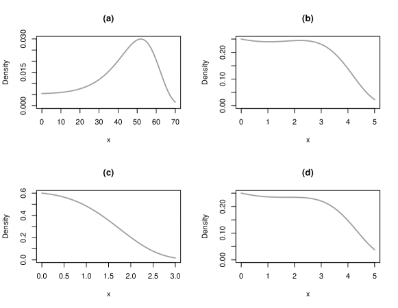
Figure 1: Shapes of the PDF of the Gompertz-Makeham distribution. For (a) we have $a=0.0005$, $b=0.1$ and $c=0.005$, for (b) we have $a=0.05$, $b=0.85$ and $c=0.2$, for (c) we have $a=0.4$, $b=0.8$ and $c=0.2$, and for (d) we have $a=0.05$, $b=0.8$ and $c=0.2$.

3.2 The Gompertz-Makeham model as a mixture

Gompertz, (1825) describes that death can be a consequence of two competing causes: one of them (non-senescent) not related to aging (e.g., accident-related mortality at young-adult ages, alcohol-related mortality at later adult ages, etc.), and another one (senescent) resulting from deterioration or increased inability to withstand destruction. As a result, the distribution of a Gompertz-Makeham random variable $X$ can be perceived as a mixture, i.e., its PDF (5) can be represented as a linear combination of two PDFs

$$f(x\,|\,a,b,c)=\pi g_{1}(x)+(1-\pi)g_{2}(x).$$

Let $F_{Y}(y\,|\,c)$ and $S_{Y}(y\,|\,c)$ denote the cumulative distribution function (CDF) and the survival function, respectively, of $Y\sim$ Exp$(c)$, while $F_{Z}(z\,|\,a,b)$ and $S_{Z}(z\,|\,a,b)$ the CDF and survival function, respectively, of $Z\sim$ Gompertz$(a,b)$. Then the corresponding PDFs are $f_{Y}(y\,|\,c)=\frac{d}{dy}F_{Y}(y\,|\,c)$ and $f_{Z}(z\,|\,a,b)=\frac{d}{dz}F_{Z}(z\,|\,a,b)$. Applying some simple algebra leads to

$$g_{1}(x)=\frac{f_{Y}(x\,|\,c)\,S_{Z}(x\,|\,a,b)}{\int\limits_{0}^{\infty}f_{Y}(t\,|\,c)\,S_{Z}(t\,|\,a,b)\,dt}\,,\hskip 28.45274ptg_{2}(x)=\frac{f_{Z}(x\,|\,a,b)\,S_{Y}(x\,|\,c)}{\int\limits_{0}^{\infty}f_{Z}(t\,|\,a,b)\,S_{Y}(t\,|\,c)\,dz}$$

and

$$\pi=\int_{0}^{\infty}f_{Y}(t\,|\,c)\,S_{Z}(t\,|\,a,b)\,dt\,,\hskip 28.45274pt1-\pi=\int_{0}^{\infty}f_{Z}(t\,|\,a,b)\,S_{Y}(t\,|\,c)\,dt$$

The survival function takes the form

$$S(x\,|\,a,b,\theta)=S_{Z}(x\,|\,a,b)\,S_{Y}(x\,|\,c)=\pi G_{1}(x)+(1-\pi)G_{2}(x)$$

with $G_{i}(x)=\int\limits_{x}^{\infty}g_{i}(z)dx$, for $i=1,2$.

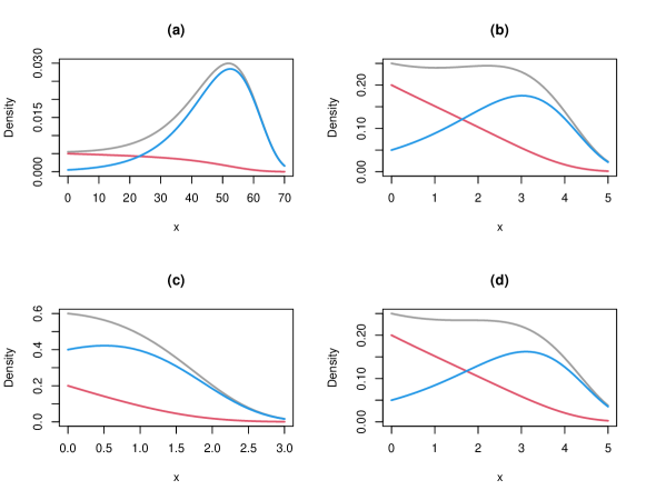
Figure 2: PDF of the Gompertz-Makeham distribution as a mixture. The grey line presents $f$, the red line indicates $g_{1}$ and the blue line represents $g_{2}$. For (a) we have $a=0.0005$, $b=0.1$ and $c=0.005$, for (b) we have $a=0.05$, $b=0.85$ and $c=0.2$, for (c) we have $a=0.4$, $b=0.8$ and $c=0.2$, and for (d) we have $a=0.05$, $b=0.8$ and $c=0.2$.

Figure 2 shows the decomposition of the Gompertz-Makeham PDF into senescent ($g_{2}$ density) and non-senescent ($g_{1}$ density) components, from which we can see how non-senescent deaths shift the maximum of the PDF (also known as modal age at death) to the left, sometimes even leading to a second peak of the distribution (panel (b) in Figure 2).

By representing the Gompertz-Makeham as a mixture of two distributions, we are able to quantify the overall proportion of non-senescent deaths, given by the quantity $\pi$, and also the proportion of non-senescent deaths at age $x$, given by the function $p(x)=\pi g_{1}(x)/[\pi g_{1}(x)+(1-\pi)g_{2}(x)]$. In the mortality context, $\pi$ can be interpreted as the overall prevalence of premature mortality, and the function $p(x)$ can be interpreted as its age-specific prevalence. For the Makeham-Gompertz model, the non-senescent deaths proportion can be expressed as $p(x)=c/\left(ae^{bx}+c\right)$. Figure 3 shows the proportion of senescent and non-senescent deaths by age in a Gompertz-Makeham model.

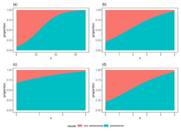
Figure 3: Proportion of senescent and non-senescent deaths by age in the Gompertz-Makeham setting. For (a) we have $a=0.0005$, $b=0.1$ and $c=0.005$, for (b) we have $a=0.05$, $b=0.85$ and $c=0.2$, for (c) we have $a=0.4$, $b=0.8$ and $c=0.2$, and for (d) we have $a=0.05$, $b=0.8$ and $c=0.2$.

The function $p(x)$ allows us to estimate the threshold age, $x^{*}$, that separates the ages with predominant non-senescent deaths from the ages with predominant senescent deaths. For the Gompertz-Makeham model,

$$x^{*}=\left\{\begin{array}[]{ l l }\frac{1}{b}\ln\frac{c}{a}&c\geq a\\ 0&c<a\\ \end{array}\right.$$

The case when $x^{*}=0$ reflects that $g_{1}(x)$ and $g_{2}(x)$ do not intersect (see, for example, panel (c) in Figure 3). In all other cases, $x^{*}$ is their intersection point, i.e., the point at which the proportion of senescent and non-senescent deaths is equal.

3.3 Makeham models as a mixture: a generalization

Let $X$ be a non-negative continuous random variable that has a Makeham hazard function given by (1). As $X$ can be written as a minimum of two random variables, we can write its PDF as

$$f(x)=c\exp\left\{-cx-H(x)\right\}+h(x)\exp\left\{-cx-H(x)\right\},$$ (6)

where $H(x)=\int\limits_{0}^{x}h(t)dt$ is the cumulative hazard function. From (6), it is easy to represent a Makeham model of the type (1) as a mixture model:

$$f(x)=\pi g_{1}(x)+(1-\pi)g_{2}(x)\,.$$ (7)

In the mortality context, we can interpret each component of the mixture. For example, the quantity

$$\pi=\int_{0}^{\infty}c\exp\left\{-cx-H(x)\right\}dx\,,$$ (8)

known as the mixing proportions (McLachlan et al., , 2019), represents the overall proportion of non-aging-related deaths, i.e., the premature mortality prevalence, while the functions

$$g_{1}(x)=\frac{c}{\pi}\exp\left\{-cx-H(x)\right\}\hskip 8.53581pt\text{and}\hskip 8.53581ptg_{2}(x)=\frac{h(x)}{1-\pi}\exp\left\{-cx-H(x)\right\}$$

are the component densities (McLachlan et al., , 2019), and represent the PDFs of the distribution of deaths of two sub-groups: $g_{1}$ is the PDF of non-aging-related (or, premature) deaths and $g_{2}$ is the PDF of aging-related (or, senescent) deaths.

By representing the class of models (1) as a mixture of two probability distributions functions, we can determine the threshold age between the premature and senescent deaths as $x^{*}=\max\{\max\{x:h(x)=c\},0\}$. We can also express the proportion of non-aging-related deaths at age $x$ as $p(x)=c/(h(x)+c)$. This function can be interpreted as the premature mortality prevalence at age $x$. Table 1 presents the closed-form expressions for the threshold age of aging-related deaths and the proportion of non-aging-related deaths at age $x$ for four well-known Makeham mortality models.

Table 1: Threshold age of aging-related deaths, $x^{*}$ and the proportion of non-aging-related deaths at age $x$, $p(x)$, in Gompertz-Makeham, gamma-Gompertz-Makeham, Beard-Makeham, Kannisto-Makeham, and Siler model settings.

Model	$h(x)$	$x^{*}$	$p(x)$
Gompertz-Makeham	$ae^{bx}$	$\frac{1}{b}\ln\frac{c}{a}$	$\frac{c}{ae^{bx}+c}$
$\Gamma$-Gompertz-Makeham	$\frac{ae^{bx}}{1+\gamma\frac{a}{b}\left(e^{bx}-1\right)}$	$\frac{1}{b}\ln\frac{c(b-a\gamma)}{a(b-c\gamma)}$	$\frac{c}{\frac{ae^{bx}}{1+\gamma\frac{a}{b}\left(e^{bx}-1\right)}+c}$
Beard-Makeham	$\frac{ae^{bx}}{1+kae^{bx}}$	$\frac{1}{b}\ln\frac{c}{a(1-kc)}$	$\frac{c}{\frac{ae^{bx}}{1+kae^{bx}}+c}$
Kannisto-Makeham	$\frac{ae^{bx}}{1+ae^{bx}}$	$\frac{1}{b}\ln\frac{c}{a(1-c)}$	$\frac{c}{\frac{ae^{bx}}{1+ae^{bx}}+c}$
Siler	$a_{1}e^{-b_{1}x}+a_{2}e^{b_{2}x}$	no closed-form	$\frac{c}{a_{1}e^{-b_{1}x}+a_{2}e^{b_{2}x}+c}$

Representing the distribution of deaths as a sum of distributions for two subpopulations, aids in studying mortality measures for each of them. For example, for each subpopulation, we can calculate the remaining life expectancy at age $x$, the force of mortality, and the modal age at death. Note that assuming a constant extrinsic risk of dying, represented by an exponential distribution, does not imply a constant force of mortality for the distribution of non-aging-related deaths. In fact, the force of mortality for this subpopulation is given by

$$h_{1}(x)=\frac{\exp\left\{-cx-H(x)\right\}}{\int_{x}^{\infty}\exp\left\{-cy-H(x)\right\}dy},$$

that is not a constant value for any non-constant function $h(x)$.

The remaining life expectancy at age $x$ is given by the function

$$e_{x}=\frac{1}{S(x)}\int_{0}^{\infty}S(x+t)\,dt\,,$$ (9)

where $S(\cdot)$ is the survival function. Substituting $S(x)=\int_{x}^{\infty}g_{1}(y)\,dy$ will yield non-senescent remaining life expectancy at age $x$ , while for $S(x)=\int_{x}^{\infty}g_{2}(y)\,dy$, (9) can be used to calculate senescent remaining life expectancy at age $x$.

We can also calculate the modal age at death for the “senescent” and “non-senescent” subpopulations, i.e., the maxima of $g_{1}(x)$ and $g_{2}(x)$. For any non-decreasing $h(x)$, the modal age at death for the non-senescent subpopulation is zero. For the senescent subpopulation (with PDF $g_{2}$), the modal age at death is the age where the overall force of mortality equals the relative derivative of $h(x)$ with respect to age:

$$h(x)+c=\frac{dh(x)/dx}{h(x)}\,.$$

Therefore, for the Gompertz-Makeham model, if $b>c$, the senescent modal age at death is given by $M_{GM}=\frac{1}{b}\,\ln\frac{b-c}{a}$, and for the gamma-Gompertz-Makeham model it is given by $M_{\Gamma GM}=\frac{1}{b}\,\ln\left(\frac{b}{a}\cdot\frac{b-a\gamma-c(1-a\gamma/b)}{b+a\gamma c}\right)$. When $c=0$, the modal age at death becomes, respectively, the Gompertz and the gamma-Gompertz modal age at death (see Missov et al., (2015) for details). The modal age at death can also be expressed for the Beard-Makeham model as $M_{BM}=\frac{1}{b}\,\ln\frac{b-c}{a(1+ck)}$, while in the Siler model setting there is no closed-form expression. Note that, given the improvements in human mortality and the rise of longevity, we may observe a decreasing trend on $c$ over time. This leads to a convergence of the overall modal age at death to the senescence one.

It is also possible to find a closed-form expression for $\pi$ in the Gompertz-Makeham and gamma-Gompertz-Makeham settings. From the Equation 8 it is easy to see that $\pi=ce_{0}$, where $e_{0}$ represents the estimated life expectancy at birth through a Makeham model. Therefore, using the life expectancy expressions presented by Castellares et al., (2020), we can easily derive the closed form for $\pi$. For the Gompertz-Makeham model, we have that

$$\pi=\frac{c}{a}\left(\frac{a}{b}\right)^{\frac{c}{b}}e^{\frac{a}{b}}\Gamma\left(-\frac{c}{b},\frac{a}{b}\right)$$

where $\Gamma(u,x)=\int_{x}^{\infty}t^{u-1}e^{-t}dx$, $x>0$ and $u\in\mathbb{R}$; that is, $\Gamma(\cdot,\cdot)$ is a complementary incomplete gamma function. For the gamma-Gompertz-Makeham model, the the closed form for $\pi$ is given by

$$\pi=\frac{c\gamma}{b+c\gamma}\,{}_{2}F_{1}\left(\frac{1}{\gamma},1;\frac{1}{\gamma}+\frac{c}{b}+1;1-\frac{a\gamma}{b}\right)$$

where ${}_{2}F_{1}(m,p;q;z)=\frac{\Gamma(q)}{\Gamma(p)\Gamma(q-p)}\int^{1}_{0}u^{p-1}(1-u)^{q-p-1}(1-zu)^{-m}du$ is the Gaussian hypergeometric function (see, for instance, Rainville, , 1960).

4 Applications

Expressing Makeham models (1) as a mixture can be advantageous for analyzing the components of mortality – the premature and the senescent ones. To illustrate these advantages, we estimate the Gompertz-Makeham model using raw death counts and exposures after age 20 from the Human Mortality Database (HMD, , 2023) for France, Italy, Japan, and Sweden, years 1947 to 2020, males and females separately.

To estimate the parameters we apply a Bayesian procedure (Gelman et al., , 2013) and assume a Poisson distribution for the death counts $D_{ijk}$, where the multi-index $ijk$ represents age $i$ in year $j$ for country $k$ (see, for example, Brillinger, , 1986). The Bayesian estimates are obtained by the mode of the posterior distributions, also known as the maximum a posteriori probability (MAP) estimate (Patricio and Missov, , 2023). The latter results from minimizing the expected canonical loss (Pereyra, , 2019).

The prior (and hyper-prior) distributions are defined as

$$a_{ijk}|\alpha_{1},\beta_{1} \sim InverseGamma(\alpha_{1},\beta_{1});$$

$$b_{ijk}|\alpha_{2},\beta_{2} \sim InverseGamma(\alpha_{2},\beta_{2});$$

$$c_{ijk}|\alpha_{3},\beta_{3} \sim InverseGamma(\alpha_{3},\beta_{3});$$

$$\alpha_{1} \sim Gamma(2,2);$$

$$\alpha_{2} \sim Gamma(2,2);$$

$$\alpha_{3} \sim Gamma(2,2);$$

$$\beta_{1} \sim Gamma(1,1);$$

$$\beta_{2} \sim Gamma(1,1);$$

$$\beta_{3} \sim Gamma(1,1)\,,$$

where $a$, $b$ and $c$ are the Gompertz-Makeham model parameters. Since the parameters are strictly positive, we choose an inverse-gamma prior distribution. The latter is characterized by a heavy tail and keeps probability further from zero than the Gamma distribution.

By specifying the prior distributions, we use numerical MCMC methods via Rstan R-package (Team et al., , 2016) to calculate the posterior distributions and the corresponding MAP estimates. The convergence criterion is evaluated by the coda R-package (Plummer et al., , 2006). The presented point estimates are MAP estimates and each of the presented intervals is a 95% Highest Density Interval (HPD interval) for the posterior distributions.

Figure 4 presents the threshold age of senescent mortality in the Gompertz-Makeham framework. For France, after the year 2000, the threshold age of senescence seems to be constant, fluctuating between ages 30 and 35 for males and around age 45 for females. Almost the same holds for Japanese males after 2010. For the other populations, after the 1990s, the threshold age shows a common increasing linear trend, suggesting that senescence has been postponed at a pace of about 4 months per year.

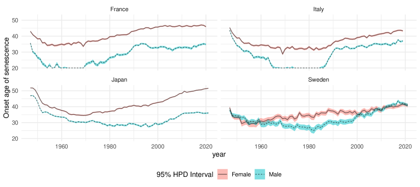
Figure 4: Threshold age between premature and senescence mortality estimated through the Gompertz-Makeham model

There is a high decrease in the prevalence of premature mortality after age 20 (see Figure 5), and its trend for all the countries and both sex leads to a constant level. For France and Italy, the latter seems to be one and the same for both sexes, while for Japan, it seems to be higher for females than for males. For Sweden, during the entire period, the prevalence for males is slightly higher than the one for females.

Figure 5: Overall prevalence of premature mortality after age 20 estimated through the Gompertz-Makeham model

Despite the overall prevalence of premature mortality converging for some countries and diverging for others, when we look at the age-specific prevalence of premature mortality (Figure 6), we see a different picture. As expected, the prevalence of premature mortality decreases with age. However, for France, while the inter-sex difference in overall prevalence seems to converge to zero, we do not observe this for the age-specific prevalence at younger ages. The same trend is seen in Italy and Japan. For Sweden, however, what we see is the opposite. The prevalence seems to be the same for males and females between ages 30 and 45, and slightly higher for males from ages 60 to 75.

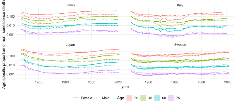
Figure 6: Age-specific prevalence of premature mortality estimated through the Gompertz-Makeham model

Over time, the age-specific prevalence of premature mortality for the French population seems to be stable for both sexes after 2000. The same holds for Japanese males after 2010 and for Italian males after 1990. For Sweden, the trend in age-specific prevalence of premature mortality seems to be identical for both sexes. Other mortality measures such as the senescent and non-senescent death distributions, their force of mortality at ages 40, 60, and 80, and their modal age of death are presented in the appendix.

5 Conclusion

In this paper, we represent Makeham mortality models as a mixture that reflects individual lifetimes in an independent competing-risk setting. The interpretation is straightforward: an individual dies either according to a baseline mortality mechanism or an exponential distribution. The mixture-model specification aids representing the distribution of deaths as a convex combination of distributions for risk-specific subpopulations. This facilitates calculating various mortality and longevity measures for each subpopulation, as well as assessing the overall and age-specific prevalence of each risk. In the case of a two-risk model when components capture senescent and premature deaths, we can estimate the threshold age that signifies the change of prevalence according to death type, from premature to senescent. We are also able to reconstruct the age-specific profile of senescent and premature (non-senescent) mortality. To illustrate these findings, we take advantage of a Bayesian approach to estimate the Gompertz-Makeham model for the French, Italian, Japanese, and Swedish populations from 1947 to 2020, after age 20. The results suggest a postponement of senescence mortality at a pace of about 4 months per year for some countries. The overall prevalence of premature mortality seems to be heterogeneous within each age group and between sexes.

6 Acknowledgements

The research leading to this publication is part of a project that has received funding from the European Research Council (ERC) under the European Union’s Horizon 2020 research and innovation program (Grant agreement No. 884328 – Unequal Lifespans). Silvio C. Patricio gratefully acknowledges the support from AXA Research Fund through funding the ”AXA Chair in Longevity Research.”

Appendix

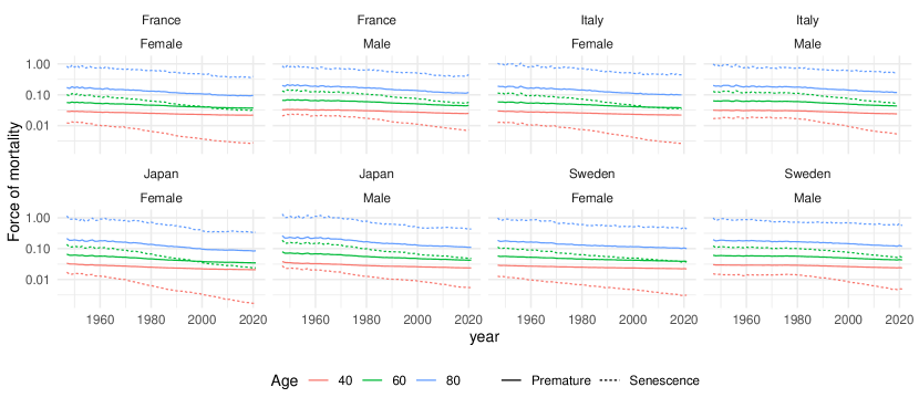
Figure 7: Estimated force of mortality at ages 40, 60, and 80 through the Gompertz-Makeham model for premature and senescent groups

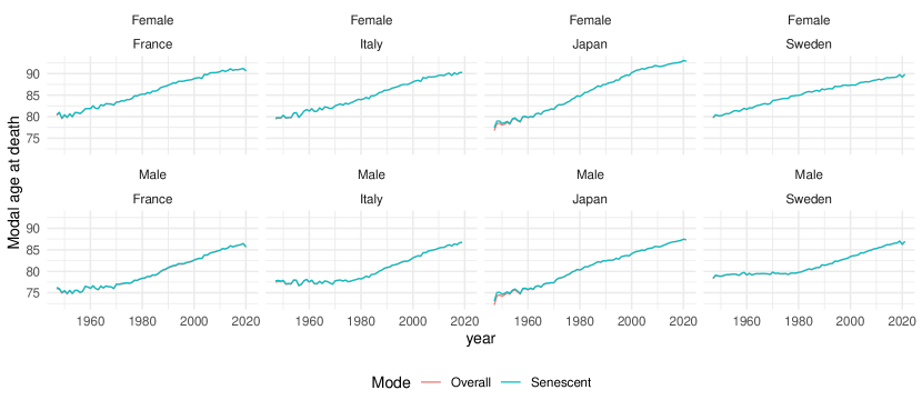
Figure 8: Estimated senescence and overall modal age at death through the Gompertz-Makeham model

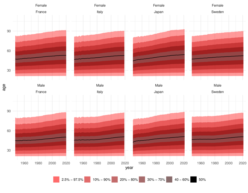
Figure 9: Estimated non-senescent death distribution after age 20 through the Gompertz-Makeham model

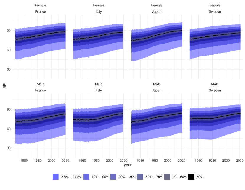
Figure 10: Estimated non-senescent death distribution through the Gompertz-Makeham model

References

- Beard, (1959) Beard, R. (1959). Notes on some mathematical mortality models. In Wolstenholme, G. and O’Connor, M., editors, The lifespan of animals, pages 802–811. Boston: Little, Brown.
- Brillinger, (1986) Brillinger, D. R. (1986). A biometrics invited paper with discussion: The natural variability of vital rates and associated statistics. Biometrics, pages 693–734.
- Castellares et al., (2022) Castellares, F., Patrício, S., and Lemonte, A. J. (2022). On the gompertz–makeham law: A useful mortality model to deal with human mortality. Brazilian Journal of Probability and Statistics, 36(3):613–639.
- Castellares et al., (2020) Castellares, F., Patrício, S. C., Lemonte, A. J., and Queiroz, B. L. (2020). On closed-form expressions to gompertz–makeham life expectancy. Theoretical Population Biology, 134:53–60.
- De Moivre, (1731) De Moivre, A. (1731). Annuities upon lives, or, the valuation of annuities upon any number of lives, as also, of reversions: To which is added, an appendix concerning the expectations of life, and probabilities of survivorship. London printed: and, Dublin re-printed, by and for Samuel Fuller.
- Gelman et al., (2013) Gelman, A., Carlin, J. B., Stern, H. S., Dunson, D. B., Vehtari, A., and Rubin, D. B. (2013). Bayesian data analysis. CRC press.
- Gompertz, (1825) Gompertz, B. (1825). Xxiv. on the nature of the function expressive of the law of human mortality, and on a new mode of determining the value of life contingencies. in a letter to francis baily, esq. frs &c. Philosophical transactions of the Royal Society of London, (115):513–583.
- HMD, (2023) HMD (2023). The human mortality database. http://www.mortality.org/.
- Jodrá, (2013) Jodrá, P. (2013). On order statistics from the gompertz–makeham distribution and the lambert w function. Mathematical Modelling and Analysis, 18(3):432–445.
- Kannisto, (1994) Kannisto, V. (1994). Development of oldest-old mortality, 1950–1990: evidence from 28 developed countries. Odense: Odense University Press.
- Kozusko and Bajzer, (2003) Kozusko, F. and Bajzer, Ž. (2003). Combining gompertzian growth and cell population dynamics. Mathematical biosciences, 185(2):153–167.
- Makeham, (1860) Makeham, W. M. (1860). On the law of mortality and the construction of annuity tables. Journal of the Institute of Actuaries, 8(6):301–310.
- Makeham, (1867) Makeham, W. M. (1867). On the law of mortality. Journal of the Institute of Actuaries, 13(6):325–358.
- Makeham, (1890) Makeham, W. M. (1890). On the further development of gompertz’s law. Journal of the Institute of Actuaries, 28(4):316–332.
- Marshall and Olkin, (2007) Marshall, A. W. and Olkin, I. (2007). Life distributions, volume 13. Springer.
- McLachlan et al., (2019) McLachlan, G. J., Lee, S. X., and Rathnayake, S. I. (2019). Finite mixture models. Annual review of statistics and its application, 6:355–378.
- Missov and Németh, (2016) Missov, T. and Németh, L. (2016). Sensitivity of model-based human mortality measures to exclusion of the makeham or the frailty parameter. Genus, 71(2-3):113–135.
- Missov et al., (2015) Missov, T. I., Lenart, A., Nemeth, L., Canudas-Romo, V., and Vaupel, J. W. (2015). The gompertz force of mortality in terms of the modal age at death. Demographic Research, 32:1031–1048.
- Norström, (1997) Norström, F. (1997). The gompertz-makeham distribution.
- Olshansky and Carnes, (1997) Olshansky, S. J. and Carnes, B. A. (1997). Ever since gompertz. Demography, 34(1):1–15.
- Patricio and Missov, (2023) Patricio, S. C. and Missov, T. I. (2023). Using a penalized likelihood to detect mortality deceleration. arXiv preprint arXiv:2301.02853.
- Pereyra, (2019) Pereyra, M. (2019). Revisiting maximum-a-posteriori estimation in log-concave models. SIAM Journal on Imaging Sciences, 12(1):650–670.
- Plummer et al., (2006) Plummer, M., Best, N., Cowles, K., Vines, K., et al. (2006). Coda: convergence diagnosis and output analysis for mcmc. R news, 6(1):7–11.
- Rainville, (1960) Rainville, E. D. (1960). Special functions. Macmillan.
- Siler, (1979) Siler, W. (1979). A competing-risk model for animal mortality. Ecology, 60(4):750–757.
- Siler, (1983) Siler, W. (1983). Parameters of mortality in human populations with widely varying life spans. Statistics in medicine, 2(3):373–380.
- Team et al., (2016) Team, S. D. et al. (2016). Rstan: the r interface to stan. R package version, 2(1):522.
- Thiele, (1871) Thiele, T. N. (1871). On a mathematical formula to express the rate of mortality throughout the whole of life, tested by a series of observations made use of by the danish life insurance company of 1871. Journal of the Institute of Actuaries, 16(5):313–329.
- Vaupel et al., (1979) Vaupel, J., Manton, K., and Stallard, E. (1979). The impact of heterogeneity in individual frailty on the dynamics of mortality. Demography, 16:439–454.