SOStab: a Matlab Toolbox for Approximating Regions of Attraction of Nonlinear Systems

Abstract

This paper presents a novel Matlab toolbox, aimed at facilitating the use of polynomial optimization for stability analysis of nonlinear systems. Indeed, in the past decade several decisive contributions made it possible to recast the difficult problem of computing stability regions of nonlinear systems, under the form of convex optimization problems that are tractable in modest dimensions. However, these techniques combine sophisticated frameworks such as algebraic geometry, measure theory and mathematical programming, and existing software still requires their user to be fluent in Sum-of-Squares and Moment programming, preventing these techniques from being used more widely in the control community. To address this issue, SOStab entirely automates the writing and solving of optimization problems, and directly outputs relevant data for the user, while requiring minimal input. In particular, no specific knowledge of optimization is needed to use it.

Keywords

Stability analysis, region of attraction, sum-of-squares programming, toolbox, Matlab.

Acknowledgement

This work was supported by the Swiss National Science Foundation under the NCCR Automation project, grant agreement 51NF40 180545, and the French company RTE, under the RTE-EPFL partnership n^∘2022-0225.

1 Introduction

Stability analysis is a crucial part of the study of dynamical systems, especially when handling safety-critical systems such as power grids, nuclear reactors, autonomous cars, railway infrastructure or airplane maneuvering systems. In particular, when the system at hand is ruled by nonlinear dynamics, a specific focus is put on computing the Region of Attraction (RoA) of secure operating points, either for finite or infinite time horizons.

When the set of admissible states (later named admissible set) is bounded (this matches realistic, physically limited systems), the “simplest” way of computing a RoA is to uniformly sample initial setpoints in the admissible set, and then each sample point is labelled as stable if, when simulated from that initial condition, the system stays in the admissible set and hits the target at the prescribed time horizon (possibly infinite, in which case one considers asymptotic properties), otherwise it is labelled as unstable. To cope with scaling issues, this computationally costly approach has been combined with Monte Carlo methods  [15, 1, 3].

A method that is dual to time-domain simulation exists, known as the direct method [19, 4, 16]. In the context of infinite time horizon, the RoA could be approximated by the largest sublevel set of a Lyapunov Function (LF). Then, the main difficulty remaining is the computation of such a LF. In some cases, physics-based heuristics can help, see e.g. [27, 6, 5] and the references therein, but in the most generic setting, it is very difficult to algorithmically compute LFs, let alone optimize over them as required when looking for a RoA.

A very promising solution to this difficult problem came from real algebraic geometry, under the form of Positivstellensatze : these theorems allow one to recast global inequality constraints on polynomials as matrix inequalities, see e.g. [23, 17, 8]. Then, looking for polynomial LFs boils down to looking for appropriate positive semidefinite matrices, even in the case of nonlinear, polynomial dynamical systems. This methodology made it possible to algorithmically compute RoAs on time horizons both infinite [11, 10, 26] and finite [7, 13, 12]. In the finite horizon setting, a byproduct of this reformulation is the convexity of the resulting optimization problem: one is faced with Linear Matrix Inequalities (LMI), which corresponds to the framework known as Lasserre’s Moment-SoS (for Sums-of-Squares) hierarchy and comes with convergence guarantees [25].

Nevertheless, approximation of finite horizon RoAs still suffers from various drawbacks: first of all, the computational complexity is polynomial in the dimension of the considered system (see [24] for details on that issue as well as possible solutions); second, many open questions remain about optimal conditioning of LMIs depending on various choices in the formulation of the problem; eventually, the issue that this article proposes to leverage, is the lack of a user-friendly interface for a practical implementation and application of the Moment-SoS hierarchy. More precisely, the existing frameworks [18, 9, 22] require the user to write, code and solve SoS programming problems whose solutions describe the RoA approximation; in contrast, the SOStab toolbox entirely automates the SoS programming part of the framework and no knowledge on the Moment-SoS hierarchy is needed to run it. Instead, the SOStab toolbox requires minimal input (namely: dynamics, state constraints, equilibrium point, time horizon, target set and a complexity parameter $d$) and outputs the stability certificate that describes the RoA approximation, as well as plots of the RoA in chosen state coordinates.

The article is organized as follows: Section 2 briefly recalls the framework of finite horizon RoA approximation with the Moment-SoS hierarchy, then Section 3 details the toolbox installation, Section 4 presents two examples of utilization of SOStab, and finally Section 5 details the toolbox structure.

2 Lasserre hierarchy for Region of attraction

In this section, the generic problem of computing the finite horizon RoA of a given target set is presented, along with the SoS framework to address it. Consider the differential system

$$\dot{\boldsymbol{x}}=\boldsymbol{f}(\boldsymbol{x})$$ (1a)

with vector field $$\boldsymbol{f}\in C^{\infty}(\mathbb{R}^{n})^{n}$$ and state constraint

$$\boldsymbol{x}(t)\in\mathbb{X}$$ (1b)

for some subset $\mathbb{X}\subset\mathbb{R}^{n}$ representing security constraints of the system.

Definition 1.

Given a time horizon $T\in(0,\infty]$ and a closed target set $\mathbb{M}\subset\mathbb{X}$, the Region of Attraction (RoA) of $\mathbb{M}$ in time $T$ is defined as

$$\mathbb{A}_{T}^{\mathbb{X}}(\mathbb{M}):=\left\{\boldsymbol{x}(0)\in\mathbb{R}^{n}\;:\begin{array}[]{c}\forall t\in[0,T),\quad\boldsymbol{x}(t)\in\mathbb{X}\\ \mathrm{dist}(\boldsymbol{x}(t),\mathbb{M})\underset{t\to T}{\longrightarrow}0\end{array}\right\}$$ (2)

Remark 2.

Definition 1 covers many frameworks, such as:

• Infinite horizon RoA ($T=\infty$, $\mathbb{X}=\mathbb{R}^{n}$, often $\mathbb{M}=\{0\}$)

• Maximal positively invariant set ($T=\infty$, $\mathbb{M}=\mathbb{X}\varsubsetneq\mathbb{R}^{n}$)

• Constrained finite horizon RoA ($T<\infty$, $\mathbb{X}$ compact)

This contribution focuses on the latter case.

We now introduce an infinite dimensional Linear Programming (LP) problem that is related to the constrained finite horizon RoA (see [7] for details):

$$W^{\star}:=\inf\;\; \int_{\mathbb{X}}w(\boldsymbol{x})\;\mathrm{d}\boldsymbol{x}$$

$$\mathrm{s.t.}\; v\in C^{\infty}(\mathbb{R}^{n+1}),w\in C^{\infty}(\mathbb{R}^{n})$$

$$w\geq 0 \text{on }\mathbb{X}$$ (3a)

$$w\geq v(0,\cdot)+1 \text{on }\mathbb{X}$$ (3b)

$$\mathcal{L}_{\boldsymbol{f}}v:=\partial_{t}v+\boldsymbol{f}^{\top}\boldsymbol{\partial}_{\boldsymbol{x}}v\leq 0 \mathbb{L}$$ on (3c)

$$v(T,\cdot)\geq 0 \text{on }\mathbb{M}$$ (3d)

where ${\mathchoice{\raisebox{0.0pt}{\scalebox{1.0}[-1.0]{$\displaystyle\mathbb{L}$}}}{\raisebox{0.0pt}{\scalebox{1.0}[-1.0]{$\textstyle\mathbb{L}$}}}{\raisebox{0.0pt}{\scalebox{1.0}[-1.0]{$\scriptstyle\mathbb{L}$}}}{\raisebox{0.0pt}{\scalebox{1.0}[-1.0]{$\scriptscriptstyle\mathbb{L}$}}}}:=[0,T]\times\mathbb{X}\Subset\mathbb{R}^{n+1}$ denotes a time-state cylinder.

Proposition 3.

Let $(v,w)$ be a feasible couple for (3). Then,

$$\mathbb{A}_{T}^{\mathbb{X}}(\mathbb{M}) \subset\{\boldsymbol{x}\in\mathbb{R}^{n}\;:\;v(0,\boldsymbol{x})\geq 0\}$$ (4a)

$$\subset\{\boldsymbol{x}\in\mathbb{R}^{n}\;:\;w(\boldsymbol{x})\geq 1\}=:\mathbb{L}(w\geq 1)$$ (4b)

Proof.

Constraint (3c) exactly means that $v$ does not increase along trajectories: $\forall\boldsymbol{x}(0)\in\mathbb{X},t\geq 0$, $v(t,\boldsymbol{x}(t))\leq v(0,\boldsymbol{x}(0))$. This, together with constraint (3d), proves (4a). (4b) directly follows from constraint (3b). ∎

With Proposition 3, constraint 3a enforces $w\geq\mathds{1}_{\mathbb{A}_{T}^{\mathbb{X}}(\mathbb{M})}$, where $\mathds{1}_{\mathbb{A}}$ denotes the boolean indicator function of $\mathbb{A}\subset\mathbb{R}^{n}$ (with value $1$ in $\mathbb{A}$ and $0$ elsewhere). Moreover, it is proven in [7] that for any minimizing sequence $(v_{k},w_{k})_{k\in\mathbb{N}}$ for (3), one has $w_{k}\underset{k\to\infty}{\longrightarrow}\mathds{1}_{\mathbb{A}_{T}^{\mathbb{X}}(\mathbb{M})}$ in the sense of $L^{1}(\mathbb{X})$, so that the volume of the approximation error $\mathbb{L}(w_{k}\geq 1)\setminus\mathbb{A}_{T}^{\mathbb{X}}(\mathbb{M})$ converges to $0$.

The Moment-SoS hierarchy allows its user to compute such a minimizing sequence, under the following assumptions.

Assumption 4.

All considered inputs are polynomial:

1. $\boldsymbol{f}\in\mathbb{R}[\mathbf{x}]^{n}$, so that $v\in\mathbb{R}[\mathrm{t},\mathbf{x}]\Longrightarrow\mathcal{L}_{\boldsymbol{f}}v\in\mathbb{R}[\mathrm{t},\mathbf{x}]$

2. $\mathbb{X}=\cap_{i=1}^{m}\mathbb{L}(g_{i}\geq 0)=:\mathbb{L}(\boldsymbol{g}\in\mathbb{R}_{+}^{m})$ with $\boldsymbol{g}\in\mathbb{R}[\mathbf{x}]^{m}$

3. $\mathbb{M}=\cap_{j=1}^{\ell}\mathbb{L}(h_{j}\geq 0)=\mathbb{L}(\boldsymbol{h}\in\mathbb{R}_{+}^{\ell})$ with $\boldsymbol{h}\in\mathbb{R}[\mathbf{x}]^{\ell}$

where $\mathbf{x}$ (resp. $\mathrm{t}$) denotes the dimension $n$ (resp. $1$) indeterminate (i.e. identity function, which can be evaluated in any state $\boldsymbol{x}\in\mathbb{R}^{n}$, resp. time $t\in\mathbb{R}$).

Then, it is possible to work with polynomial Sums-of-Squares (SoS), with the following definitions.

Definition 5.

Let $p\in\mathbb{R}[\mathbf{x}]$. Then, considering $g_{0}:=1$,

• $p$ is SoS iff $p=q_{1}^{2}+\ldots+q_{N}^{2}$, $q_{1},\ldots,q_{N}\in\mathbb{R}[\mathbf{x}]$

• $p\in\mathcal{Q}(\boldsymbol{g})$ iff $p=s_{0}\,g_{0}+\ldots+s_{m}\,g_{m}$, $s_{0},\ldots,s_{m}$ SoS

• $p\in\mathcal{Q}_{k}(\boldsymbol{g})$ iff $p\in\mathcal{Q}(\boldsymbol{g})$ with $\max(\deg s_{i}\,g_{i})\leq 2k$

Since SoS polynomials are nonnegative by design, it is clear from Definition 5 that any $p\in\mathcal{Q}_{k}(\boldsymbol{g})$ (resp. $\mathcal{Q}_{k}(\boldsymbol{h})$) is nonnegative on $\mathbb{X}$ (resp. $\mathbb{M}$), which gives access to a strenghtening of problem (3):

$$W^{\star}_{k}:=\inf\;\; \int_{\mathbb{X}}w(\boldsymbol{x})\;\mathrm{d}\boldsymbol{x}$$

$$\mathrm{s.t.}\; v\in\mathbb{R}[\mathrm{t},\mathbf{x}],w\in\mathbb{R}[\mathbf{x}]$$

$$w \in\mathcal{Q}_{k}(\boldsymbol{g})$$ (5a)

$$w-v(0,\mathbf{x})-1 \in\mathcal{Q}_{k}(\boldsymbol{g})$$ (5b)

$$-\mathcal{L}_{\boldsymbol{f}}v \in\mathcal{Q}_{k}(\boldsymbol{g},(T-\mathrm{t})\,\mathrm{t})$$ (5c)

$$v(T,\mathbf{x}) \in\mathcal{Q}_{k}(\boldsymbol{h})$$ (5d)

where ${\mathchoice{\raisebox{0.0pt}{\scalebox{1.0}[-1.0]{$\displaystyle\mathbb{L}$}}}{\raisebox{0.0pt}{\scalebox{1.0}[-1.0]{$\textstyle\mathbb{L}$}}}{\raisebox{0.0pt}{\scalebox{1.0}[-1.0]{$\scriptstyle\mathbb{L}$}}}{\raisebox{0.0pt}{\scalebox{1.0}[-1.0]{$\scriptscriptstyle\mathbb{L}$}}}}=\mathbb{L}((T-\mathrm{t})\,\mathrm{t}\geq 0)\times\mathbb{X}=\mathbb{L}((\boldsymbol{g},(T-\mathrm{t})\,\mathrm{t})\in\mathbb{R}_{+}^{m+1})$.

Problem (5) consists in looking for feasible $(v,w)$ for (3) under the form of polynomials, restricting inequality constraint (3x) into SoS constraint (5x), x$=$a–d. The advantage of this new problem is that the decision variables are now finite dimensional vectors of coefficients, and the SoS constraints can be recast as LMIs [17]. Thus, assuming knowledge of the moments of the Lebesgue measure on $\mathbb{X}$ (i.e. being able to integrate polynomials on $\mathbb{X}$, e.g. if $\mathbb{X}$ is a ball or a box), one is able to solve (5) on a standard computer, provided that $n$ and $k$ are small enough to make the LMIs tractable.

As the new feasible space is strictly included in the former, there is a relaxation gap: $\forall k\in\mathbb{N},\ W^{\star}<W^{\star}_{k}$. However, it is proved in [7] that, under mild assumptions (easily satisfied if $\mathbb{X}$ and $\mathbb{M}$ are bounded), $W^{\star}_{k}\underset{k\to\infty}{\longrightarrow}W^{\star}$. More specifically, if $(v_{k}^{\star},w_{k}^{\star})$ is an optimal solution of (5), then the volume of the approximation error $\mathbb{L}(w_{k}^{\star}\geq 1)\setminus\mathbb{A}_{T}^{\mathbb{X}}(\mathbb{M})$ converges to $0$ when $k$ goes to infinity. Thus, solving instances of (5) gives access to converging outer approximations of the RoA.

This framework comes with several extensions (not detailed here) among which:

• Approximation of a free final time RoA [7]

  $$\mathbb{A}_{[0,T]}^{\mathbb{X}}(\mathbb{M}):=\left\{\boldsymbol{x}(0)\in\mathbb{R}^{n}\;:\begin{array}[]{c}\forall t\in[0,T],\;\;\boldsymbol{x}(t)\in\mathbb{X}\\ \exists\,t\in[0,T],\;\;\boldsymbol{x}(t)\in\mathbb{M}\end{array}\right\}$$

• Inner RoA approximation [13]

• RoA approximation for non-polynomial (trigonometric) dynamics [12]

• Maximal positively invariant set approximation [14, 21]

3 Installation of the toolbox

SOStab is a freeware subject to the General Public Licence (GPL) policy. It is available for Matlab and can be downloaded at

https://github.com/droste89/SOStab

SOStab requires YALMIP [18], as well as a semidefinite solver. Mosek [20] is used by default, but it can be replaced by any other solver, provided they are installed and interfaced through YALMIP.

4 Getting started with two examples

4.1 A standard polynomial system

Consider the reversed-time Van der Pol oscillator, as in [13]:

$$\begin{pmatrix}\dot{x_{1}}\\ \dot{x_{2}}\end{pmatrix}=\begin{pmatrix}-2x_{2}\\ 0.8x_{1}+10(x_{1}^{2}-0.21)x_{2}\end{pmatrix}$$ (6)

The stable equilibrium $\boldsymbol{x}_{eq}$ of the system (such that $\boldsymbol{f}(\boldsymbol{x}_{eq})=\mathbf{0}$ and $\lim_{t\to\infty}\boldsymbol{x}(t)=\boldsymbol{x}_{eq}$ if $\boldsymbol{x}(0)$ is close enough to $\boldsymbol{x}_{eq}$) is at the origin. SOStab is designed to approximate the finite horizon region of attraction of a neighbourhood of $\boldsymbol{x}_{eq}$. The problem is first defined with:

     VdP = SOStab([0;0], [1.1;1.1]);     

Here the first argument is the equilibrium $\boldsymbol{x}_{eq}=(0,0)$, the second argument gives admissible deviation $\Delta\boldsymbol{x}=(1.1,1.1)$ such that the admissible set is given by $\mathbb{X}=[\boldsymbol{x}_{eq}\pm\Delta\boldsymbol{x}]$ (where for $\boldsymbol{a},\boldsymbol{b}\in\mathbb{R}^{n}$, $[\boldsymbol{a}\pm\boldsymbol{b}]:=[a_{1}-b_{1},a_{1}+b_{1}]\times\ldots\times[a_{n}-b_{n},a_{n}+b_{n}]$).

The dynamics of the system are then defined:

     VdP.dynamics= [-2*VdP.x(2); 0.8*VdP.x(1) + 10*(VdP.x(1)^2 - 0.21)*VdP.x(2)];     

where VdP.x denotes the variable $\boldsymbol{x}$ of the system (defined inside the class creation).

Now that the problem is defined, the outer approximation of the time $T=1$ RoA of $\mathbb{M}=\{\boldsymbol{x}\in\mathbb{R}^{n}\;:\;\|\boldsymbol{x}-\boldsymbol{x}_{eq}\|^{2}\leq 0.5^{2}\}$ is calculated using the following command:

     d = 12;         T = 1;         epsilon = 0.5;  [vol, vc, wc] = VdP.SoS_out(d, T, epsilon);     

$T$ is the time horizon of the approximation and $d=2k$ is the maximum degree of the polynomial variables.

It returns the volume of the calculated RoA appproximation and the coefficients of the polynomial variables $v^{\star}_{k}$ and $w^{\star}_{k}$.

Once the optimization is done, the results can be plotted in two dimensions using:

     VdP.plot_roa(1, 2, ’outer’);     where the first two arguments indicate the indices of the plotted variables (respectively in abscissa and ordinate). The string “outer” indicates that the outer approximation RoA is plotted. For inner RoA approximation [13], the commands are

     [vol, vc, wc] = VdP.SoS_in(d, T, epsilon);  VdP.plot_roa(1, 2, ’inner’,1);     Here the last argument with value 1 is an optional argument that asks SOStab to also represent the target set in the figure. This gives the plot represented in Figure 1, which reproduces results presented in [7, Figure 2] and [13, Figure 3].

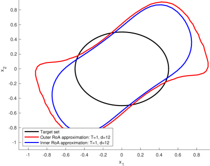
Figure 1: Inner and outer RoA approximations for the Vanderpol system.

The 3d-plots of polynomials $v^{\star}_{k}$ and $w^{\star}_{k}$ can be displayed with:

     VdP.plot_v(1, 2, ’outer’);  VdP.plot_w(1, 2, ’outer’);     of course, one can also represent the certificates $v^{\star}_{k}$ and $w^{\star}_{k}$ obtained in inner approximation, simply by setting the last argument at ’inner’.

4.2 A non-polynomial power system

Consider an electrical power network made of synchronous machines connected in a cycle, along with its second reduced order model [2]:

$$\dot{\theta}_{1} =\omega_{1},\qquad\dot{\theta}_{2}=\omega_{2}$$ (7a)

$$\dot{\omega}_{1} =-\sin\theta_{1}-0.5\sin(\theta_{1}-\theta_{2})-0.4\,\omega_{1}$$ (7b)

$$\dot{\omega}_{2} =-0.5\sin\theta_{2}-0.5\sin(\theta_{2}-\theta_{1})-0.5\,\omega_{2}+0.05$$ (7c)

with state variable $\boldsymbol{\sigma}=(\theta_{1},\theta_{2},\omega_{1},\omega_{2})\in\mathbb{R}^{4}$, stable equilibrium given by $\boldsymbol{\sigma}_{eq}=(0.02,0.06,0,0)$ and non-polynomial dynamics. Here, a preprocessing $\boldsymbol{x}:=\boldsymbol{\varphi}(\boldsymbol{\sigma})$ is required from the user to recast the dynamics under a polynomial form; each phase variable $\theta_{i}$ is represented by its sine and cosine, through the change of variables:

$$\boldsymbol{x}=(\sin\theta_{1},\cos\theta_{1},\sin\theta_{2},\cos\theta_{2},\omega_{1},\omega_{2})\in\mathbb{R}^{6}$$ (8)

Then, one can prove (similarly to e.g. [2, 12]) that the new variable $\boldsymbol{x}$ has polynomial dynamics: $\dot{\boldsymbol{x}}=\boldsymbol{f}(\boldsymbol{x})$, with $\boldsymbol{f}\in\mathbb{R}[\mathbf{x}]^{6}$, and equilibrium $\boldsymbol{x}_{eq}=\boldsymbol{\varphi}(\boldsymbol{\sigma}_{eq})$. Then, the RoA approximation problem is defined with

     powsys = SOStab([sin(0.02); cos(0.02); sin(0.06); cos(0.06);0;0],                  [1;1;1;1;pi;pi],                      [1,2;3,4]);     Here the first two arguments are identical as in the polynomial setting: they indicate the equilibrium point and admissible deviation for the variable with polynomial dynamics. The third argument is specific to systems with trigonometric dynamics, and identifies the indices of sines and cosines of phase variables $\theta_{i}$ in the recasted $\boldsymbol{x}$: here the line [1,2] (resp. [3,4]) means that $x_{1}=\sin\theta_{1}$ and $x_{2}=\cos\theta_{1}$ (resp. $x_{3}=\sin\theta_{2}$ and $x_{4}=\cos\theta_{2}$). Then, powsys.dynamics, powsys.SoS_outer and powsys.SoS_inner are the same as in the polynomial setting. However, the code for plotting is slightly modified in its first argument:

     powsys.plot_roa([1,2],[3,4],’outer’, 1);     Here, instead of giving indices as first two arguments, the user inputs pairs of indices related to sine and cosine functions of phase variables; the toolbox then automatically plots the RoA depending on the physically relevant phase variable rather than its trigonometric representations. This yields, in the case of our power system, the plot of Figure 2, which reproduces (at a lower degree) the result of [12, Figure 2].

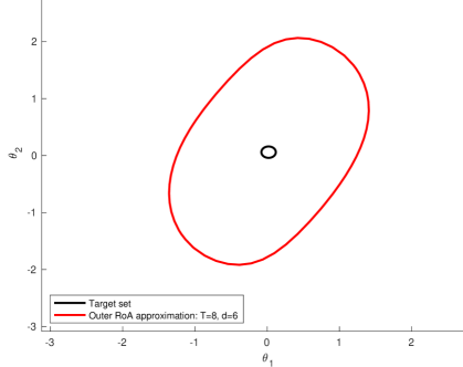
Figure 2: Outer RoA approximation for the power system.

Remark 6.

One could also represent the RoA in a phase space (e.g. in the $(\theta_{1},\omega_{1})$ plane) with the following command, which mixes a pair of indices (for $\theta_{1}$) and a single index (for $\omega_{1}$):

     powsys.plot_roa([1,2],5,’outer’, 1);     

5 Properties and methods

5.1 Formulation of the problem input

The problem formulated by the user and given to the toolbox must have a specific form. First of all, it must be already in polynomial form, which means that only products of variables are allowed. The toolbox requires the following input:

$$\dot{\boldsymbol{x}}=\boldsymbol{f}(\boldsymbol{x}),\quad\boldsymbol{f}\in\mathbb{R}[\mathbf{x}]^{n}$$

$$\mathbb{X}=[\boldsymbol{x}_{eq}\pm\Delta\boldsymbol{x}],\quad\Delta\boldsymbol{x}\in(0,\infty)^{n}$$

$$\boldsymbol{x}_{eq}\in\mathbb{R}^{n},\quad T>0,\quad\varepsilon>0,$$

$$\mathbb{M}=\{\boldsymbol{x}\in\mathbb{R}^{n}:\|\mathbf{A}(\boldsymbol{x}-\boldsymbol{x}_{eq})\|^{2}\leq\varepsilon^{2}\}$$

$$\mathbf{A}\in\mathbb{R}^{n\times n};\quad\mathbf{A}^{\top}=\mathbf{A},\quad\det\mathbf{A}=1$$

Specifying $\mathbf{A}$ is optional, with default value $\mathbf{A}=\mathbf{I}_{n}$ (identity matrix). An optional input, needed when the dynamics of the system include trigonometric dynamics depending on $N$ phase variables $\theta_{1},\ldots,\theta_{N}$, is the list of indices of sine and cosine recastings of these variables, given under the form of a $N\times 2$ matrix $\mathbf{Z}$: the first (resp. second) column represents indices of the sines (resp. cosines) of $\theta_{1},\ldots,\theta_{N}$, each line corresponding to a given phase variable $\theta_{i}$ (see example in Section 4.2).

The toolbox will center and normalize the problem, essentially in order to avoid artifacts related to the evaluation of high degree monomials $x_{i}^{\alpha_{i}}$ with $|x_{i}|>1$ and $\alpha_{i}\gg 1$.

5.2 Definition of a problem instance

A SOStab class is defined with three arguments: the equilibrium point of the problem $\boldsymbol{x}_{eq}$, the range of the admissible set of the trajectories $\Delta\boldsymbol{x}$ – defining an admissible set $[\boldsymbol{x}_{eq}\pm\Delta\boldsymbol{x}]$ – as well as the optional matrix $\mathbf{Z}$ defining phase variables (when needed). The two vectors $\boldsymbol{x}_{eq}$ and $\Delta\boldsymbol{x}$ must have the same length, and when applicable $\mathbf{Z}$ should have 2 columns (and as many rows as there are phase variables), with non-repeating natural integers.

     RoA_pb = SOStab(x_eq, delta_x); % or  RoA_pb = SOStab(x_eq, delta_x, angle_ind);     

Remark 7.

Note that the Moment-SoS hierarchy framework can be used with other admissible sets $\mathbb{X}$ (e.g. ellipsoids, possibly independent from the equilibrium). SOStab focuses on boxes to match the intuition of physical limits on a system: most often, each state variable $x_{i}$ is required to stay in a given range $\Delta x_{i}$. However, in some cases, such description induces bad conditioning in the considered LMIs. Future versions of SOStab will include a broader range of admissible sets $\mathbb{X}$.

The initial call creates an instance of the class, and defines the following properties:

• dimension: dimension of the problem (number of variables)

• x_eq: first argument of the call, the equilibrium state of the system

• delta_x: the range around the equilibrium defining the feasible set

• angle_eq: the vector $\boldsymbol{\theta}_{eq}$ – the equilibrium angles – recalculated from the values of their sine and cosine (empty if no phases are involved)

• angle_ind: the indices of sine and cosine functions in the recast variable $\boldsymbol{x}$, given as last input of SOStab call (empty if no phases are involved)

• x: a YALMIP sdpvar polynomial object, of the dimension of the problem. It represents the variable $\boldsymbol{x}$ and is used by the user to define the dynamics of the system

• t: sdpvar polynomial of size 1, representing the time variable, which can be needed to define the dynamics of the system (if non-autonomous)

• D, the matrix $\mathbf{D}$ of the variable change used in the toolbox to normalize the system

• invD, the inverse $\mathbf{D}^{-1}$ of the matrix $\mathbf{D}$

• solver, the choice of the solver used in the optimization, defined as Mosek by default

• verbose, the value of the verbose parameters of the YALMIP optimization calls, defined at 2 by default

• dynamics, a YALMIP polynomial defining the polynomial dynamics $\boldsymbol{f}$ of the system

The dynamics of the system are added into the class by the user by allocating a value to RoA_pb.dynamics. The dynamics must be a vector of size dimension, each row corresponding to the dynamics of one variable. To define dynamics, one will use the sdpvar object x and created inside the class. For instance, defining $(\dot{x_{1}},\dot{x_{2}})=(-x_{1},-x_{2}^{3})$ would be:

     RoA_pb.dynamics = [-RoA_pb.x(1); -RoA_pb.x(2)^3];     

The solver used for the optimization can be modified after defining the class, as well as the verbose parameter. Using sedumi with no verbose would be:

     RoA_pb.solver = ’sedumi’; RoA_pb.verbose = 0;     

5.3 Additional properties

Additionnal properties are related to a specific solution of the optimization problem. They are calculated at each call of the optimization and stored until the next call, i.e. each of them correponds to the previous optimization call:

• d$=2k$, the degree of the polynomials in (5)

• A, the matrix defining the target set (identity by default)

• epsilon, the positive radius of the target set

• vcoef_outer, the coefficients of the solution $v^{\star}_{k}$ for the last calculated outer approximation of the ROA

• wcoef_outer, the coefficients of the solution $w^{\star}_{k}$ for the last calculated outer approximation of the ROA

• vcoef_inner, the coefficients of the solution $v^{\star}_{k}$ for the last calculated inner approximation of the ROA

• wcoef_inner, the coefficients of the solution $w^{\star}_{k}$ for the last calculated inner approximation of the ROA

• solution, a volume approximation of the last calculated ROA, ie the solution of the optimization problem

Note that the first three properties are also arguments of the optimization call. These properties are changed during the call of the function (and reused for the plotting for example).

5.4 Workings of the toolbox

As stated before, the Moment-SoS hierarchy consists in solving instances of (5), which requires to follow a number of steps, related to real algebraic geometry and optimization:

1. Defining the geometric characteristics of the problem (polynomial dynamics $\boldsymbol{f}$, time horizon $T$, admissible and target sets $\mathbb{X}$ and $\mathbb{M}$)

2. Defining an algebraic description of these geometric characteristics: polynomials $\boldsymbol{g}\in\mathbb{R}[\mathrm{x}]^{m}$ s.t. $\mathbb{X}=\mathbb{L}(\boldsymbol{g}\in\mathbb{R}_{+}^{m})$ and $\boldsymbol{h}\in\mathbb{R}[\mathrm{x}]^{\ell}$ s.t. $\mathbb{M}=\mathbb{L}(\boldsymbol{h}\in\mathbb{R}_{+}^{\ell})$

3. Coding a method to integrate polynomials over $\mathbb{X}$ (i.e. computing the moments of the Lebesgue measure on $\mathbb{X}$)

4. Writing problem (5) with explicit formulation of constraints (5a-5d); this requires introducing SoS certificates $s_{i}$ as in Definition 5 as decision variables

5. Recasting SoS constraints as LMIs, solving the resulting SDP problem and converting the solution back to the polynomial framework

6. Extracting the corresponding certificates $v^{\star}_{k},w^{\star}_{k}$ and using them to characterize and plot relevant representations of the computed RoA approximation.

Existing frameworks [18, 9, 22] have been designed to automate step 5 which appears in all instances of SoS programming. As a result, they are very flexible in their use, but they also require their user to perform steps 1–4 and 6 by hand, which requires solid knowledge in SoS programming and can be an occasion for many human errors, typos and bugs (especially in step 4); hence their use is usually not smooth, even for experts. In contrast, with SOStab, only step 1 is left to the user, and all the other operations are automatically performed by the toolbox.

More precisely, intrinsic properties of the dynamical system are defined as presented in section 5.2, and then settings for finite horizon RoA are the input of methods SoS_in and SoS_out: an optional matrix $\mathbf{A}$ (by default $\mathbf{A}=\mathbf{I}_{n}$) and a real $\varepsilon>0$ to define the target $\mathbb{M}$, an even degree $d=2k$ for $v$, $w$ and the SoS certificates, and a time horizon $T\in(0,\infty)$; with this, steps 2–5 are performed through a call to YALMIP, for inner and outer RoA approximation respectively, and output an optimal value vol and the coefficients of the optimal polynomials $v^{\star}_{k}$ and $w^{\star}_{k}$. Currently, the inner approximation has limitations on some of the instances tested, due to the algebraic representation of the boundary $\partial\mathbb{X}$.

Regarding step 6: plot_roa takes as inputs the two indices $i,j$ of the variables on which to project the RoA, a string to choose between ’inner’ and ’outer’ approximation, and four optional arguments: an int (1 or 0) – 0 by default – to choose to plot the target or not, two strings indicating the axes names – $x_{i}$ and $x_{j}$ by default – and the size of the plotting mesh – $(40,40)$ by default. It plots the expected slice of the ROA, with all other variables at equilibrium. If both inner and outer approximations are called sequentially for the same variables, the two plots will appear on the same figure.

plot_v and plot_w take the same inputs as plot_roa. They respectively plot the graph of $v^{\star}_{k}$ and $w^{\star}_{k}$ in 3D (with non-selected variables at equilibrium).

Remark 8.

In the current version of the toolbox, when using an optional argument, one should also specify all optional arguments that appear before in the method call.

6 Conclusion and future works

This contribution presented a new Matlab Toolbox called SOStab, which aims at helping a non-expert in polynomial optimization to use the frameworks developed in [7, 13, 12] through a plug-and-play interface. Taking only ODE-related inputs (such as dynamics, admissible and target sets, time horizon) as well as an even complexity parameter $d=2k$, the toolbox fully automates writing, recasting and solving the corresponding SoS programming problem, and outputs stability certificates $v^{\star}_{k}$ and $w^{\star}_{k}$ which can be evaluated at a given initial condition to assess its stability. This is in sharp contrast with existing frameworks [18, 9, 22] which require the users to take upon themselves the burden of properly designing and coding the SoS programming problems that correspond to their RoA approximation problem. The benefits of this contribution are the following:

1. Knowledge on SoS programming becomes optional to use the Lasserre hierarchy for RoA approximation

2. The probability of bug related to human errors is drastically limited, as the input from the user is sharply reduced

3. The toolbox comes with a plug-and-play design that allows one to repeat multiple experiments, reproduce existing results from the literature and solve new problems

However, some limitations remain to be leveraged. For instance, while convex, SDP problems can be ill-conditioned, which sometimes results in poor numerical behavior with $w^{\star}_{k}\simeq 1$ and meaningless plots. It is possible to rescale SoS constraints to mitigate that phenomenon, although finding the appropriate rescalings is non-trivial. Also, inner RoA approximation requires an algebraic representation of the boundary $\partial\mathbb{X}$ of the admissible set $\mathbb{X}$ [13], and while choosing a box is the most physically relevant (and the easiest to integrate polynomials on), it induces some numerical difficulties that would not arise if $\mathbb{X}$ were described by a single polynomial. This can be solved either by improving the inner approximation scheme on a box, or by changing the admissible set $\mathbb{X}$. Another issue related to the numerical convergence of Lasserre’s hierarchy, is that the canonical basis of monomials is far from being the best choice (see the last concluding statement in [7]) and a way to work with other bases of polynomials (especially orthonormal bases) would help improving all existing results. Future works on the SOStab class will include:

1. Improving the inner approximation scheme to increase the accuracy of each relaxation

2. Supporting richer admissible $\mathbb{X}$ and target $\mathbb{M}$ sets, such as ellipsoids, $\ell^{p}$-balls, annuli…

3. Extending the toolbox to other frameworks, e.g. [14, 21]

4. Supporting bases of polynomials other than monomials (Chebyshev, Legendre, trigonometric polynomials)

5. Exporting the toolbox to other softwares compatible with existing SDP solvers, such as Julia or Python.

References

- [1] George J. Anders. Probability concepts in electric power systems. Wiley, 1989.
- [2] Marian Anghel, Federico Milano, and Antonis Papachristodoulou. Algorithmic construction of Lyapunov functions for power system stability analysis. IEEE Transactions on Circuits and Systems I: Regular Papers, 60(9):2533–2546, 2013.
- [3] Franz Bamer, Denny Thaler, Marcus Stoffel, and Bernd Markert. A Monte Carlo simulation approach in non-linear structural dynamics using convolutional neural networks. Frontiers in Built Environment, 7, 2021.
- [4] Evgeny A. Barbashin and Nikolai N. Krasovsky. On the stability of motion as a whole. Doklady Akademii Nauk SSSR, pages 453–456, 1952.
- [5] Hsiao-Dong Chiang. Direct Methods for Stability Analysis of Electric Power Systems. Wiley, 2011.
- [6] Hsiao-Dong Chiang, Chia-Chi Chu, and G. Cauley. Direct stability analysis of electric power systems using energy functions: theory, applications, and perspective. Proceedings of the IEEE, 83(11):1497–1529, 1995.
- [7] Didier Henrion and Milan Korda. Convex computation of the region of attraction of polynomial control systems. IEEE Transactions on Automatic Control, 59(2):297–312, 2013.
- [8] Didier Henrion, Milan Korda, and JEan B. Lasserre. The Moment-SOS Hierarchy. World Scientific, 2021.
- [9] Didier Henrion, Jean B. Lasserre, and Johann Löfberg. GloptiPoly 3: moments, optimization and semidefinite programming. Optimization Methods and Software, 24(4-5):761–779, 2009.
- [10] Shinsaku Izumi, Hiroki Somekawa, Xin Xin, and Taiga Yamasaki. Estimating regions of attraction of power systems by using sum of squares programming. Electrical Engineering, 100:2205–2216, 2018.
- [11] Zachary W. Jarvis-Wloszek. Lyapunov based analysis and controller synthesis for polynomial systems using sum-of-squares optimization. PhD thesis, University of California, 2003.
- [12] Cédric Josz, Daniel K Molzahn, Matteo Tacchi, and Somayeh Sojoudi. Transient stability analysis of power systems via occupation measures. In 2019 IEEE Power & Energy Society Innovative Smart Grid Technologies Conference (ISGT), pages 1–5. IEEE, 2019.
- [13] Milan Korda, Didier Henrion, and Colin N Jones. Inner approximations of the region of attraction for polynomial dynamical systems. IFAC Proceedings Volumes, 46(23):534–539, 2013.
- [14] Milan Korda, Didier Henrion, and Colin N. Jones. Convex computation of the maximum controlled invariant set for polynomial control systems. SIAM Journal on Control and Optimization, 52(5):2944–2969, 2014.
- [15] P.R.S. Kuruganty and Roy Billinton. A probabilistic assessment of transient stability. International Journal of Electrical Power & Energy Systems, 2(2):115–119, 1980.
- [16] Joseph Pierre LaSalle. Some extensions of Liapunov’s second method. IRE Transactions on Circuit Theory, 7:520–527, 1960.
- [17] Jean B. Lasserre. Moments, Positive Polynomials and Their Applications. Imperial College Press, 2010.
- [18] Johan Löfberg. Pre- and post-processing sum-of-squares programs in practice. IEEE Transactions on Automatic Control, 54(5):1007–1011, 2009.
- [19] Alexandr M. Lyapunov. The general problem of stability of motion. PhD thesis, University of Kharkov, 1892.
- [20] MOSEK ApS. The MOSEK optimization toolbox for MATLAB manual. Version 10.0., 2022.
- [21] Antoine Oustry, Matteo Tacchi, and Didier Henrion. Inner approximations of the maximal positively invariant set for polynomial dynamical systems. IEEE Control Systems Letters, 3(3):733–738, 2019.
- [22] Antonis Papachristodoulou, James Anderson, Giorgio Valmorbida, Stephen Prajna, Peter Seiler, Pablo A. Parrilo, Matthew M. Peet, and Declan Jagt. SOSTOOLS – Sum of Squares Optimization Toolbox for MATLAB.
- [23] Mihai Putinar. Positive polynomials on compact semi-algebraic sets. Indiana University Mathematics Journal, 42(3):969–984, 1993.
- [24] Matteo Tacchi. Moment-SOS hierarchy for large scale set approximation. Application to power systems transient stability analysis. PhD thesis, INSA de Toulouse, June 2021.
- [25] Matteo Tacchi. Convergence of Lasserre’s hierarchy: the general case. Optimization Letters, 16(3):1015–1033, 2022.
- [26] Matteo Tacchi, Marian Anghel, Soumya Kundu, Sifeddine Benahmed, and Carmen Cardozo. Power system transient stability analysis using sum of squares programming. In Power Systems Computation Conference, 2018.
- [27] V. Vittal, A.N. Michel, and A.A. Fouad. Power system transient stability analysis: formulation as nearly hamiltonian systems. Circuits System Signal Process, 3(1):105–122, 1984.