Physical cool-core condensation radius in massive galaxy clusters

Abstract

Aims. We investigate the properties of cool cores in an optimally selected sample of 37 massive and X-ray-bright galaxy clusters, with regular morphologies, observed with Chandra. We started by measuring the density, temperature, and abundance radial profiles of their intracluster medium (ICM). From these independent quantities, we computed the cooling ($t_{\rm cool}$), free-fall ($t_{\rm ff}$), and turbulence ($t_{\rm eddy}$) timescales as a function of radius.

Methods. By requiring the profile-crossing condition, $t_{\rm cool}/t_{\rm eddy}=1$, we measured the cool-core condensation radius, $R_{\rm ccc}$, within which the balancing feeding and feedback processes generate the turbulent condensation rain and related chaotic cold accretion (CCA). We also constrained the complementary (quenched) cooling flow radius, $R_{\rm qcf}$, obtained via the condition $t_{\rm cool}=25\times t_{\rm ff}$, that encompasses the region of thermally unstable cooling.

Results. We find that in our our massive cluster sample and in the limited redshift range considered ($1.3\times 10^{14}<M_{500}<16.6\times 10^{14}\,M_{\odot}$, $0.03<z<0.29$), the distribution of $R_{\rm ccc}$ peaks at $\sim$ 0.01 $r_{500}$ and the entire range remains below $\sim$ 0.07 $r_{500}$, with a very weak increase with redshift and no dependence on the cluster mass. We find that $R_{\rm qcf}$ is typically three times larger than $R_{\rm ccc}$, with a wider distribution, and growing more slowly along $R_{\rm ccc}$, according to an average relation $R_{\rm qcf}\propto R_{\rm ccc}^{0.46}$, with a large intrinsic scatter.

Conclusions. We suggest that this sublinear relation can be understood as an effect of the micro rain of pockets of cooled gas flickering in the turbulent ICM, whose dynamical and thermodynamical properties are referred to as ”macro weather.” Substituting the classical ad-hoc cool-core radius $R_{\rm 7.7\,Gyr}$, we propose that $R_{\rm qcf}$ is an indicator of the size of global cool cores tied to the long-term macro weather, with the inner $R_{\rm ccc}$ closely tracing the effective condensation rain and chaotic cold accretion (CCA) zone that feeds the central supermassive black hole (SMBH).

1 Introduction

The hot intracluster medium (ICM) is the largest baryonic component in groups and clusters of galaxies (Gonzalez et al. 2013). It is observable in the X-ray band thanks to its strong Bremsstrahlung continuum emission plus emission lines from highly ionized elements, and it shows temperatures from 1 keV (groups) to more than 10 keV (massive clusters). The density profile of the ICM is usually fitted with the $\beta$ profile (Cavaliere & Fusco-Femiano 1978), consisting of a flat core and rapidly decreasing outskirts. However, in many clusters, the central electron density is not accurately described by a single $\beta$ profile, but is observed to be sharply peaked, reaching values significantly larger than the typical $n_{\rm e}$ $\thicksim$ 10^-3 cm^-3. In these cases, a double $\beta$ profile is needed to fit the X-ray surface brightness (as known from ROSAT observations Xue & Wu 2000), effectively defining a central core where the ICM cooling time, $t_{\rm cool}$ $\propto kT/n_{e}$, is significantly lower than the typical age of the cluster. This implies that a large amount of gas should cool completely on a short timescale (typically less than 1 Gyr) due to radiative losses, leading to a massive cooling flow with a mass deposition rate of the order of several hundreds up to thousands M_⊙ yr^-1. Such large values are obtained directly from the brightness profile under the assumption of subsonic flow and constant pressure, as per the so-called ”isobaric cooling flow” model (Fabian & Nulsen 1977; Fabian 1994).

The X-ray luminosity in cluster cores is dominated by the hottest ICM component (above a few keV), while the coldest one contributes only a few percent of the total, while being rich in emission lines. At variance with the ”isobaric cooling flow” scenario, high-resolution spectroscopy of bright clusters with XMM–Newton have not shown any evidence for the multiphase, line-rich gas predicted by the isobaric cooling model. Instead, it has been observed that the majority of the ICM typically reaches a temperature plateau at about one-third of the virial value (Kaastra et al. 2001; Peterson et al. 2001; Tamura et al. 2001; Donahue & Voit 2004), while the cold gas below this floor is virtually absent. In this framework, the old paradigm of ”cooling flow” has been abandoned in favour of the ”cool core” scenario (Molendi & Pizzolato 2001). Despite some amount of cooling gas, possibly associated with star-forming episodes in the central galaxy, is still allowed by the observations, the upper limits to the spectroscopic mass-deposition rate values are at least one order of magnitude lower than the rates expected by isobaric cooling flow models (McNamara & O’Connell 1989; Makishima et al. 2001; Edge 2001; Edge & Frayer 2003; McNamara & Nulsen 2007). Recently, spatially resolved spectral analyses of cool cores have confirmed that the central, isobaric mass-deposition rates are significantly lower than the star-formation rates observed in the hosted brightest cluster galaxy (BCG; Molendi et al. 2016). On the other hand, the more convincing cooling flow candidates are limited to only one well-documented case (the Phoenix cluster, see McDonald et al. 2012; Tozzi et al. 2015; Pinto et al. 2018; McDonald et al. 2019).

This observational evidence strongly supports the presence of some heating mechanism that prevents the bulk of the ICM from cooling below about one-third of the virial temperature in the cool core. This is now considered a standard condition of the ICM in cool-core clusters, which represent $\sim 70\%$ of the low-redshift population of X-ray flux-limited sample, according to Hudson et al. (2010). On the other hand, some amount of cold and multiphase gas is now commonly observed in the submm and optical band in star forming regions of the BCG thanks to ALMA (e.g., McNamara et al. 2014; Russell et al. 2017; Temi et al. 2018; Tremblay et al. 2018; Rose et al. 2019; North et al. 2021) and MUSE (e.g., Olivares et al. 2019, 2022; Maccagni et al. 2021), respectively. The presence of multiphase gas suggests that short-lived cooling flows raining all the way down onto the central supermassive black hole (SMBH) in the BCG have time to replenish the cold gas reservoir before being quenched by the ensuing SMBH feedback process. In summary, we are well aware that cool cores are physical systems where the cooling process is counterbalanced by some global heating mechanism that strongly suppresses the mass deposition rate, while still allowing some amount of gas to leak out of the hot phase with a timescale regulated by a complex feeding (cooling) and feedback (heating) cycle (Gaspari & Sa̧dowski 2017). A comprehensive and systematic comparison of the spectroscopic mass deposition rate to the star formation rate in the BCG and the presence of molecular gas in the cluster core, significantly extending the small sample explored in Molendi et al. (2016), would provide very effective constraints on the baryonic cycle in clusters. In addition, the detection of very diffuse, low-temperature ICM in the center of non-cool-core clusters by the next generation of X-ray bolometers, may provide support for a scenario in which cool-core clusters rapidly switch into the non cool-core phase and vice versa (see Molendi et al. 2023).

Many heating mechanisms have been proposed in the past two decades, among them: thermal conduction (Zakamska & Narayan 2003), viscous dissipation of sound waves (Ruszkowski et al. 2004), supernova feedback (Domainko et al. 2004), turbulence combined with conduction (Dennis & Chandran 2005), cosmic ray–ICM interaction (Guo & Oh 2008; Yang et al. 2019), and feedback from jets and outflows from the central active galactic nucleus (AGN; e.g., McNamara & Nulsen 2007; Gaspari et al. 2012b; Barai et al. 2016; Wittor & Gaspari 2020; McKinley et al. 2022). In particular, the last process is considered the most likely contributor on the basis of the well-documented interactions between radio jets and the surrounding ICM. The large amount of mechanical energy associated with the cavities carved into the ICM by the radio jets may be eventually transformed into thermal energy of the ICM (Blanton et al. 2010, for a review) and may stimulate, at the same time, the cooling of some fraction of the gas (Gaspari et al. 2020, for a review). Therefore, no matter how many mechanisms are contributing, the central AGN is expected to play an important role in regulating cooling, ultimately inducing tight scaling relations between the SMBH and AGN as well as the hot halo properties (Gaspari et al. 2019; Pasini et al. 2021).

In this work we investigate key physical radii that delimit the spherical regions where different phases of the complex baryon cycle are actually taking place, such as the cool-core condensation radius ($R_{\rm ccc}$) and the quenched cooling flow radius ($R_{\rm qcf}$). In Section 2, we introduce and discuss our definition of $R_{\rm ccc}$ and $R_{\rm qcf}$. In Section 3, we derive the typical timescales of relevant processes occurring in galaxy clusters. In Section 4, we describe the selection of the sample of galaxy clusters observed with Chandra and used in this work. In Section 5, we discuss the key parameter represented by the turbulent velocity dispersion of the warm and cold phase of the diffuse baryons. In Section 6, we describe data reduction and our analysis strategy. Our results are described in Section 7, where we show deprojected timescale profiles in each cluster as a function of radius and we measure the $R_{\rm ccc}$ and the $R_{\rm qcf}$ values, followed by an investigation of their distribution across the cluster sample. The physical implication of our findings are discussed in Section 8 and our conclusions are summarized in Section 9. Throughout the paper, the cosmological model of reference is a $\Lambda$CDM with parameters $H_{0}$ = 67.8 km s^-1 Mpc^-1, $\Omega_{\Lambda}$ = 0.692 and $\Omega_{m}$ = 0.308 (Planck Collaboration et al. 2016). Quoted errors and upper limits correspond to a 1-$\sigma$ confidence level.

2 Physical definition of cool-core condensation and quenched cooling-flow radius

From the observational point of view, it has been well established that the presence of radio nuclear activity is closely associated with the presence of a cool core (Dunn & Fabian 2006; Sun 2009). The interactions between the relativistic electrons and the thermal electrons of the ICM have been thoroughly studied in spectacular images of few nearby clusters such as Perseus (Fabian et al. 2003b), Hydra A (McNamara et al. 2000), and few other clusters at intermediate redshift (Blanton et al. 2011; Ehlert et al. 2011); in addition, the presence of cavities in the ICM has been explored up to $z\thicksim 1.2$ (Hlavacek-Larrondo et al. 2015). However, while the energy budget associated with cavities is sufficient to switch off the cooling in all the observed cases, the physical mechanism by which the energy of the jet is transferred isotropically to the ICM is still an issue of debate. Possible mechanisms include turbulence (e.g., Gaspari 2015) or weak shocks (e.g., Fabian et al. 2003a; Mathews et al. 2006) driven by the radio-mode activity of the central galaxy. The key issue here is to identify a process that regularly transforms an impulsive and directional energy input of the jet into a gentle heating, smoothly distributed in time and space, to finally shape the regular ICM thermodynamical properties observed in cool-core clusters.

All these details cannot be resolved in most cool-core clusters and, therefore, the actual physical processes can hardly be constrained from the macroscopic X-ray quantities such as luminosity and temperature. In recent years, several independent efforts have been devoted to achieve an efficient observational diagnostics to classify clusters according to the presence of a cool core and, at the same time, to understand the dominant physical processes. The many quantities used to define a cool core are all related to the thermodynamical properties of the ICM but they are associated with different physical processes: surface brightness excess or cuspiness (Santos et al. 2008), the temperature gradient (Sanderson et al. 2006; Burns et al. 2008), a steep iron abundance profile (De Grandi et al. 2004; Rasera et al. 2008), steep slopes of central entropy (Pratt et al. 2010), low central cooling time (O’Hara et al. 2006), classical mass deposition rate (Chen et al. 2007), and (clearly) the slope of the electron density profile (Hudson et al. 2010). All these diagnostics are obtained by combining the same three independent X-ray observables: surface brightness, temperature, and line emission.

In a comprehensive overview, Hudson et al. (2010) concluded that the central cooling time is one of the best diagnostics for identifying and characterizing cool cores. Furthermore, Gaspari et al. (2018) showed that the ratio of the cooling time over the turbulence eddy turnover timescale $C\equiv t_{\rm cool}/t_{\rm eddy}\sim 1$ is a key diagnostic for the condensation extent of the multiphase rain occurring via chaotic cold accretion (hereafter, CCA). In other words, whenever the $C$-ratio approaches unity there is enough turbulence and quick cooling to directly drive non-linear instabilities. This is confirmed by studies obtained with high-resolution radio/optical telescopes (Gaspari et al. 2018; Olivares et al. 2019, 2022), which show that multiphase filamentary structures can be observed within the region enclosed by $t_{\rm cool}/t_{\rm eddy}\approx 1$. In this region, the turbulent mixing rate is expected in part to balance the pure cooling flow, in part to drive direct nonlinear thermal instability that then ends up generating a rainfall. As shown by theoretical studies, the ICM can be seen as a hierarchical thermodynamic system that follows a chaotic, top-down multiphase condensation cascade (Gaspari et al. 2017; Voit et al. 2017). Therefore, we assume that an appropriate timescale for feedback is provided by the turbulence timescale, $t_{\rm eddy}$. In this work, we leverage these findings to identify the approximately spherical region within which the nonlinear multiphase CCA rain and the triggered feedback response are very effective, via the following condition:

$$C\equiv t_{\rm cool}(R_{\rm ccc})/t_{\rm eddy}(R_{\rm ccc})=1.$$ (1)

This relation effectively defines the cool-core condensation radius, $R_{\rm ccc}$. Within $R_{\rm ccc}$, we expect direct turbulence instability to be driving localized flickering precipitation and, therefore, the condensation of the light rain that may be responsible for accretion events onto the central SMBH in the BCG, and thus leading to star formation episodes in the BCG.

At the same time, we can identify a region where we assume thermally unstable cooling may ensue from linear perturbations by establishing a threshold in the ratio of the cooling, $t_{\rm cool}$, and the free-fall time $t_{\rm ff}$ (e.g., Field 1965). Voit et al. (2015b) found that the minimum value of $t_{\rm cool}$/$t_{\rm ff}$ fluctuate around values of $10-20$, concluding that cold clouds start to precipitate out of hot-gas atmospheres when $t_{\rm cool}$ drops to ten times $t_{\rm ff}$. Later, Hogan et al. (2017) showed that the minimum of the $t_{\rm cool}$/$t_{\rm ff}$ ratio in a large sample of observed clusters with constrained nebular emission (tracing the condensed cool gas) is bound between 10 and 40, with few values below 10, which is also supported by hydrodynamical simulations with self-regulated AGN jet feedback (Gaspari et al. 2012b).

Therefore, we argue that an average ratio $\equiv t_{\rm cool}$/$t_{\rm ff}\sim 25$, despite a large scatter, is a reasonable proxy for tracing the initial growth of linear thermal instability (TI) in heated cooling flows, while a value of 10 traces the lower bound of such a criterion. Overall, we define a quenched cooling flow radius (and use it here) when the following condition is met:

$$t_{\rm cool}(R_{\rm qcf})=25\times\,t_{\rm ff}(R_{\rm qcf})\,.$$ (2)

In this framework, the quantity $R_{\rm qcf}$ is expected to be an alternative definition to the ”classical” cool-core radius defined on the basis of the cooling time. Indeed, the radius below is often used, whereby the cooling time is shorter than the reference value of 7.7 Gyr, $R_{\rm classic}\equiv R_{\rm 7.7\,Gyr}$; Hudson et al. 2010).

Overall, we expect the two newly defined core radii to trace physical transitions from a macro-scale X-ray emitting ICM atmosphere delimited by a ”classical” cool core radius to a region where a quenched cooling inflow could potentially develop ($<R_{\rm qcf}$), and, eventually, to a region where precipitation and feedback are actively vigorous ($<R_{\rm ccc}$). To explore the behaviour of these two spatial scales, we sought to measure $R_{\rm qcf}$ and $R_{\rm ccc}$ in an optimally selected sample of massive clusters observed with the Chandra satellite.

3 Timescales in the ICM of massive Galaxy Clusters

In this section, we define the timescale for physical processes relevant to the ICM, which is treated as an optically thin plasma in collisional ionization equilibrium, despite occasional out-of-equilibrium phases that may potentially be reached. However, treating the ICM in steady equilibrium is a fitting approximation and would not bias our results. As previously discussed, we will also assume spherical symmetry, as a requirement that will affect the sample selection in certain ways, as discussed in Section 4.

3.1 Cooling time

The ICM X-ray emission is composed of thermal bremsstrahlung (free-free emission) plus line emission from ions of heavy elements. The X-ray luminosity density (energy emitted per unit time at a unit volume) can therefore be written as $L_{X}\approx n_{e}^{2}\Lambda(T,Z)$, where $n_{\rm e}$ is the electron density and $\Lambda(T,Z)$ is the cooling function, which depends on the temperature of both radiative processes and is also related with the abundance, $Z,$ of heavy elements in the ICM (see Figure 3 of Peterson & Fabian 2006). For the hot ICM ($kT>2$ keV), the bremsstrahlung emission dominates and the approximation $\Lambda(T)\propto T^{1/2}$ is usually adopted. When temperatures are low, the number of ions (and therefore the number of possible transitions) strongly increases. As a consequence, the enhanced contribution from line emission significantly affects the cooling function. This regime is particularly relevant in cool cores, where low temperatures are always associated with high metallicity, often reaching supersolar values (De Grandi et al. 2004; Liu et al. 2020). Therefore, to describe the cooling efficiency of the ICM accurately at different radii, the full cooling function must be taken into account.

The main energy loss of the ICM is the thermal radiative emission, which is mostly observed in the classic 0.5-10 keV X-ray band for the temperature range we are considering here. Therefore, the cooling time is typically defined as the timescale after which the ICM entirely loses its internal energy via bremsstrahlung radiation, down to the point when the gas eventually recombines and starts loosing energy through other radiative processes. An effective way to estimate the ICM cooling time is obtained by dividing the gas internal energy by the luminosity density of the plasma. We can therefore express the internal energy as $(3/2)\,nkT$, obtaining the following for the cooling time:

$$t_{\rm cool}\simeq\frac{3}{2}\frac{nkT}{n_{\rm e}n_{\rm i}\Lambda(Z,T)},$$ (3)

where $\Lambda(Z,T)$ is the cooling function for gas with a specific abundance, $Z,$ and temperature, $kT$. In this work, we compute the cooling function interpolating the values reported in Sutherland & Dopita (1993). We note that here we adopt a definition of cooling time based on the internal energy rather than the enthalpy $(5/2)nkT$ (Peterson & Fabian 2006). The factor of $5/2$ is assumed to account for the inclusion of the extra work-term arising from perfect spherically symmetric isobaric compression. However, the $5/2$ value should be considered as an upper limit, since (under realistic conditions) there is no perfect isobaric compression and any contribution from turbulence or AGN heating brings it near the pure 3/2 factor, as shown in Figure 5 of Gaspari (2015).

For temperatures $kT\gtrsim 2$ keV (and metallicity $0.3\,Z_{\sun}$), only Bremsstrahlung emission is relevant for such clusters, thus $t_{\rm cool}$ is well approximated by the expression (see Cavagnolo et al. 2009):

$$t_{\rm cool}\simeq 10^{8}\,{\rm yr}\left(\frac{K}{10\,\rm keV\,cm^{2}}\right)^{3/2}\left(\frac{kT}{\rm 5\,keV}\right)^{-1}\,,$$ (4)

where $K\equiv kT/n_{\rm e}^{2/3}$ is the astrophysical (electron) entropy (Ponman et al. 1999; Tozzi & Norman 2001). We note that using a higher solar metallicity reduces the normalization in Equation 4 by only 30%. Moreover, hydrodynamical simulations predict that this cooling time ought to have a radial dependence approximated by a power law with a slope of $\sim$ 1.3 (Ettori & Brighenti 2008).

3.2 Free-fall time

The free-fall time is defined as the timescale of an object falling towards the center of the cluster without any pressure support or any deceleration due to viscosity (Binney & Tremaine 1987). The free-fall time can be written as:

$$t_{\rm ff}=\sqrt{\frac{2r}{g(r)}}=\sqrt{\frac{2r\rho_{g}}{dP/dr}}=\sqrt{\frac{2r^{3}}{GM}}\,,$$ (5)

where $M$ is the total mass within a spherical radius, $r$. The free-fall time, therefore, depends on the total mass and not on the properties of the ICM, such as density. The total mass profile $M(<r)$ can, in turn, be computed directly from the ICM applying the condition of hydrostatic equilibrium, which requires the knowledge of the density and temperature profiles of the ICM:

$$M(<r)=\,-\,\frac{r^{2}}{G\rho_{g}}\frac{{\rm d}P}{{\rm d}r}=\,-\,r\frac{kT(r)}{\mu m_{p}G}\left(\frac{{\rm d}\log(n_{e})}{{\rm d}\log(r)}+\frac{{\rm d}\log(kT)}{{\rm d}\log(r)}\right)\,,$$ (6)

where $kT(r)$ is the deprojected temperature profile of the ICM, $n_{e}(r)$ the deprojected electron density profiles, $\mu$ is the mean molecular weight of ICM (which is usually assumed to be $\mu$ = 0.6). and $m_{p}$ is the proton mass.

3.3 Turbulence timescale

A number of processes, such as cluster mergers, galaxy motions, and AGN feedback, are capable of producing turbulence in the ICM. The mechanical energy associated with these processes is very high and X-ray observations clearly show that the ICM is significantly affected by it (Iapichino et al. 2010; Gaspari et al. 2014; Liu et al. 2015; Lau et al. 2017; Wittor & Gaspari 2020). Combining X-ray and radio observations, it has been shown that radio jets injects bubbles of relativistic electrons that create cavities within the ICM on scales of 10-100 kpc (McNamara et al. 2005; Diehl et al. 2008; Blanton et al. 2011; Hlavacek-Larrondo et al. 2015; Yang et al. 2019). The expectation is that a relevant fraction of the mechanical energy associated with the buoyant rise of inflated bubbles (or with bulk motions of infalling halos) will transfer into the ICM and eventually produce turbulence. Measurements of turbulence in cluster cores have been reported, in particular, via the power spectra of density fluctuations (Schuecker et al. 2004; Sanders et al. 2010; Gaspari & Churazov 2013; Zhuravleva et al. 2014; Hofmann et al. 2016; Simionescu et al. 2019). The only measurement of turbulence in the ICM at high spectral resolution has been provided by the Hitomi mission (Hitomi Collaboration et al. 2016), which showed a few 100 km s^-1 in turbulent velocities in Perseus cluster. The ultimate observational evidence of the amplitude and distribution of turbulence in the ICM will be provided in the next future by X-ray high-resolution spectra, obtained with the X-ray spectrometers Resolve onboard XRISM and X-IFU onboard Athena.

Following Gaspari et al. (2018), we can estimate the turbulence characteristic timescale via the eddy turnover/mixing time, such as

$$t_{\rm eddy}=2\pi\frac{r^{2/3}L^{1/3}}{\sigma_{v,L}}\,,$$ (7)

where $L$ is the energy-injection scale and $\sigma_{v,L}$ is the typical turbulent velocity measured at the injection scale. The injection scale, $L,$ is related to the AGN feedback influence region and can be approximated via the typical observed size covered by the pair of cavities inflated in the ICM (alternatively, by the extent of the H$\alpha$ nebula). A phenomenological scaling for $L$ is obtained from the large sample by Shin et al. (2016), with $L\sim 10\,(kT/1\,\rm keV)^{2}$ kpc (see also Gaspari et al. 2019). Given the strong dependence on the average temperature, it can reach values as high as $\sim$ 200 kpc, as in the case of MS 0735.6+7421 (Vantyghem et al. 2014).

The other relevant parameter, namely, the turbulent velocity dispersion, $\sigma_{v,L}$, is preferentially taken from the literature (Gaspari et al. 2018; Olivares et al. 2019) whenever a direct measurement is available. If no measurements are available, we consider a range of values chosen (as detailed in Section 5). Another assumption here is that we assume that the three-dimensional velocity dispersion $\sigma_{v,L}$ is obtained multiplying by $\sqrt{3}$ the line-of-sight velocity dispersion of the warm and cold gas measured in (Gaspari et al. 2018; Olivares et al. 2019), which implies isotropic turbulence. This may not be true when violent gas sloshing is present. In fact, during the initial phase, sloshing-induced turbulence may have larger velocity dispersion in the plane of sloshing motion. On the one hand, estimating and removing the effects of gas sloshing is beyond the capability of the current analysis. On the other hand, we argue that its impact is limited. This assumption is based on the fact that sloshing develops on much larger time scales (see ZuHone et al. 2013; Zuhone & Roediger 2016), while the AGN feedback is self-regulated on duty cycles corresponding to $\sim 1-10$ Myr (see Gaspari et al. 2012a). Therefore, we expect that the main contribution to the turbulence level is provided by the AGN feedback, while sloshing may boost the turbulence on time scales ranging 0.1 – a few Gyr (for minor and major mergers, respectively; see discussion in Lau et al. 2017). Within this framework, we adopt the assumption of isotropic turbulence bearing in mind that $t_{\rm eddy}$ can be slightly affected by anisotropic bulk motions of the ICM.

4 Cluster sample selection

The term ”cool core” typically refers to the central region of a cluster, approximately in hydrostatic equilibrium, which shows a density profile significantly peaked toward the center, the temperature profile increasing with the radius on a scale of $\thicksim$ 50 kpc, an iron abundance profile decreasing with radius on the same scale, and, therefore, a short cooling time. In the absence of a recent major merger, a cool core invariably hosts a BCG at its center.

To achieve a robust measurement of radial timescale profiles down to a few kpc, we decided to perform our study with Chandra data, thanks to its angular resolution unparalleled among current X-ray facilities, which allows us to resolve a scale below 10 kpc virtually at redshifts up to $z\sim 1$. In this way, the effective resolution of our analysis will be determined solely by the surface brightness of the ICM emission and the exposure depth of the data. To optimally select a sample of clusters for our study, we considered the Chandra archive to collect all the targets where we can measure the timescale profiles well inside the potential cool core region with an accuracy sufficient to identify the transition radii, $R_{\rm qcf}$ and $R_{\rm ccc}$. As a rule of thumb, we know that the typical size of cool cores is around 40 kpc (Santos et al. 2008), therefore, as the first criterion, we require enough counts within this radius to extract at least two rings with a minimum of 3000 net counts each in the 0.5-7 keV band. This will allow us to measure the temperature with an error lower than $\sim 20\%$ in the spatial bins within 40 kpc.

On the other hand, we also need to measure temperature and density out to 300–400 kpc, in order to track how timescale profiles behave before approaching the cooling region. Due to the limited Chandra field of view (16^′ $\times$ 16^′ for ACIS-I, 8^′ $\times$ 8^′ for ACIS-S), the requirement to reach $\sim$ 400 kpc in the FOV translates in a conservative lower limit $z>0.03$ and $z>0.1$ for ACIS-I and ACIS-S, respectively. We also require $z<0.3$ to have at least a width of 3 arcsec for the minimum ring width of $\sim 15$ kpc.

We start from a total sample of 1144 galaxy clusters or groups, consisting of all the publicly available archival data under this category. Our requirement on the redshift range brings this number down to 456 clusters. After applying our criterion on the net number of counts and removing those clusters that strongly depart from a relaxed, a spherical morphology after a visual inspection, we obtained a total of 37 clusters at 0.03 $<z<$ 0.3 satisfying our criteria. With the knowledge that a simple visual inspection does not guarantee a relaxed dynamics, with this step, we excluded all the clusters with disturbed morphologies that would make a spherical deprojection unreliable. We also note that the requirement on the net counts within 40 kpc strongly favors cool-core clusters, since to reach the same angular resolution in our spectral analysis, non-cool-core clusters need to have a significantly deeper exposure to match the same number of photons in the inner 40 kpc as compared to cool-core clusters. Therefore, non cool-core clusters are expected to be underrepresented in our final sample. However, since we are aiming at investigating the correlation between core properties and other observables (and not the distribution across the cluster population), the predominance of cool-core clusters does not strongly affect our conclusions. The list of clusters, with redshift, position, ObsID, and effective total exposure time after data reduction, is shown in Table 1. We note that not all the available exposures for each target are used. In particular, we removed all the off-centered pointings (aiming at the cluster outskirts) and we discarded some pointings with very low exposures ($\sim 5$ ks) or with an observation date very far from the bulk of the other observations (which would imply a significantly different effective area). Usually, we keep observations in both ACIS detectors, but in some cases, we discarded the observations in one of the detectors when the corresponding exposure is a minority of the total exposure time; this was done to achieve a simpler spectral analysis at the cost of a negligible loss in signal.

Table 1: Sample of clusters observed with Chandra and satisfying the criteria defined in Section 3. Column 1: Cluster name; column 2: Redshift; column 3: R.A. of cluster center; column 4: Declination of the cluster center; column 5: Obsid used in the analysis (ACIS-S and ACIS-I observations are marked with ”S” and ”I,” respectively); column 6: Exposure time after data reduction; column 7: Net photon counts within 40 kpc in the 0.5-7.0 keV band.

Cluster	z	RA	DEC	ObsID	$t_{\rm exp}(\rm ks)$	Net photon counts
A2199	0.0302	16h28m38.4s	+39d33m03.6s	497,498(S)	158.3	78044.9
				10748,10803
				10804,10805(I)
A496	0.0329	04h33m37.92s	-13d15m43.2s	931,3361,4976(S)	104.0	60790.1
2A0335+096	0.0363	03h38m40.56s	+09d58m12s	919,7939,9792(S)	103.0	93744.0
A2589	0.0414	23h23m57.12s	+16d46m44.4s	3210,6948,7190	92.3	5413.7
				7340(S)
MKW3S	0.0450	15h21m51.84s	+07d42m32.4s	900 (I)	57.3	51816.4
Hydra A	0.0548	09h18m05.7s	-12d05m44s	4969,4970(S)	98.82	214993.0
A85	0.0551	00h41m45.84s	-09d22m44.4s	904,15173,15174	195.2	45290.9
				16263,16264 (I)
A2626	0.0553	23h36m30.48s	+21d08m45.6s	3192,16136(S)	135.6	11042.6
A133	0.0566	01h02m56.4s	-22d08m27.6s	2203(S)	154.3	34627.3
				9897,13518(I)
SERSIC159-03	0.0580	23h13m58.32s	-42d43m33.6s	1668(S),11758(I)	107.7	16595.1
A1991	0.0587	14h54m31.44s	+18d38m31.2s	3193(S)	38.3	28575.4
A3112	0.0753	03h17m57.6s	-44d14m16.8s	2216,2516(S),13135(I)	66.4	10847.0
A2029	0.0773	15h10m56.16s	+05d44m38.4s	891,4977(S)	126.9	167014.4
				6101,10434,10435
				10436,10437(I)
A2597	0.0852	23h25m19.68s	-12d07m26.4s	922,6934,7329(S)	151.64	79071.1
A3921	0.0928	22h50m02.88s	-64d21m54s	4973(I)	29.4	3211.7
A2244	0.0968	17h02m42.72s	+34d03m36s	4179(S)	57.0	21639.1
RXCJ1558.3-1410	0.0970	15h58m21.84s	-14d09m57.6s	9402(S)	40.1	18550.6
PKS0745-19	0.1028	07h47m31.2s	-19d17m38.4s	12881(S)	118.1	175872.9
RXCJ1524.2-3154	0.1028	15h24m12.72s	-31d54m25.2s	9401(S)	40.9	33188.5
RXCJ0352.9+1941	0.1090	03h52m58.8s	+19d40m58.8s	10466(S)	27.2	11261.1
A1664	0.1283	13h03m42.48s	-24d14m42s	1648,7901,17172	110.0	11873.3
				17173,17557,17568(S)
A2204	0.1522	16h32m47.04s	+05d34m33.6s	499(S)	96.82	74069.5
				6104,7940(I)
A907	0.1527	09h58m21.36s	-11d03m39.6s	535,3185,3205(I)	106.1	8276.3
HerculesA	0.1550	16h51m08.16s	+04d59m34.8s	5796,6257(S)	97.1	5347.0
RXJ2014.8	0.1612	20h14m51.6s	-24d30m21.6s	11757(S)	19.91	16628.1
A1204	0.1706	11h13m18s	+17d36m10.8s	2205(I)	23.6	7863.1
Zw2701	0.2140	09h52m48.96s	+51d53m06s	12903(S)	95.8	11649.9
RXCJ1504-0248	0.2153	15h04m08.4s	-02d48m25.2s	4935,5793,17197	150.0	13281.1
				17669,17670(I)
RXCJ1459.4-1811	0.2357	14h59m28.8s	-18d10m44.4s	9428(S)	39.6	9297.7
4C+55.16	0.2411	08h34m54.96s	+55d34m22.8s	4940(S)	96.0	16780.3
CL2089	0.2492	09h00m36.96s	+20d53m42s	10463(S)	40.6	9861.6
RXJ2129.6+0005	0.2499	21h29m40.08s	+00d05m24s	552,9370(I)	40.0	3797.8
A1835	0.2532	14h01m01.92s	+02d52m40.8s	6880,6881,7370(I)	194.0	44128.0
RXCJ1023.8-2715	0.2533	10h23m50.16s	-27d15m21.6s	9400(S)	36.7	10127.0
CL0348	0.2537	01h06m49.2s	+01d03m21.6s	10465(S)	48.9	10354.3
MS1455.0+2232	0.2578	14h57m14.4s	+22d20m38.4s	543,4192(I)	101.7	17724.3
ZW3146	0.2906	10h23m39.6s	+04d11m09.6s	909,9371(I)	86.2	10715.8

5 Turbulent velocity dispersion estimate

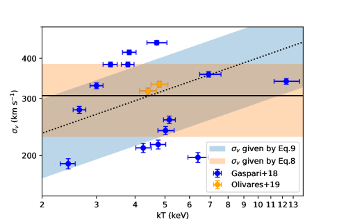
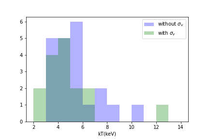
Figure 1: Top panel: Turbulent velocity values measured in the warm or cold phase by Gaspari et al. (2018, blue points) and Olivares et al. (2019, orange points). The reference dotted line $\sigma\propto T^{1/3}$ corresponds to Equation 9, with the cyan-shaded area showing the 1 $\sigma$ uncertainty. The solid lined corresponds to the constant average value given by Equation 8, with the orange-shaded area showing its 1 $\sigma$ uncertainty. Bottom panel: the histogram distribution of the clusters with $\sigma_{v}$ measurement (blue) and of the complementary subsample (green).

We collected all the measurements available (in the literature) of the turbulent velocity at a particular injection (5-10 kpc) of the warm or cold phase for our selected clusters, converting the line-of-sight measurement into a three-dimensional (3D) value, assuming isotropic turbulence, as discussed in Section 3.3. Here, we assume that the turbulent velocity dispersion of the ICM is very close to the value measured for the cold and warm medium. This correlation is shown to have a slope and a normalization close to unity, with a scatter of $\sim$30% (see Fig 1 in Gaspari et al. 2018). We retrieved average ensemble measurements of $\sigma_{v}$ for 14 clusters from Gaspari et al. (2018) that overlap with our sample. From Olivares et al. (2019), we collected two other new measurements. We note that Olivares et al. (2019) provided other measurements in clusters overlapping with Gaspari et al. (2018); however, they are tied to pencil-beam values, while ensemble values, such as those listed in Table 1 of Gaspari et al. (2018), should be used here, since they better trace the dynamical and thermodynamical properties of the turbulent medium, which we indicate as ”macro weather.”

Therefore, 40% of our sample has values of 3D $\sigma_{v}$ and associated uncertainties (directly derived from the observed line-of-sight $\sigma_{v}$) that can be directly inserted in Equation 7 for the corresponding cluster. In Figure 1 (left panel), we show the 16 clusters in the $\sigma_{v}-kT$ plane. We note a large intrinsic scatter with no clear trend with the temperature. Such a large scatter likely dilutes any weak dependence on the (core-excised) temperature, given the current low statistics. The measured values are scattered in the range $200<\sigma_{v}<400$ km/s, with the average value and rms given by:

$$\langle\sigma_{v}\rangle=306\pm 78\,\,{\tt km/s}\,.$$ (8)

The constant value $\langle\sigma_{v}\rangle$ and its uncertainty are shown as an orange shaded area in Figure 1 (left panel). The question is then whether the turbulent velocity in the clusters without direct measurements can be assumed to be within this range. As a first step, we compared the temperature distribution of the 18 clusters with measured $\sigma_{v}$ to that of the 25 clusters without $\sigma_{v}$. The two distributions are shown in Figure 1 (right panel), where it is possible to see that the clusters without $\sigma_{v}$ measurement are hotter (hence, more massive) than those with $\sigma_{v}$. Therefore, assuming a constant values for $\sigma_{v}$, despite the large uncertainty, may not fully track the dependence on the temperature-mass scale.

The dependence of $\sigma_{v,L}$ on the mass scale has been investigated only in a few works. Gaspari et al. (2018) find $\sigma_{v}\propto M^{0.2}\propto T_{\rm x}^{0.3}$ in the larger sample of 72 groups and clusters, by leveraging ensemble-beam optical spectra, which are shown to linearly trace hot-gas turbulent velocities within a 0.13 dex scatter. By using a completely different method and band based on X-ray brightness and density fluctuations in 33 groups and clusters, Hofmann et al. (2016) retrieved a slightly negative slope in the hot-gas turbulent Mach numbers (defined as $\sigma_{v}/c_{\rm s}$, with the sound speed being $c_{\rm s}\propto T_{\rm x}^{1/2}$), translating again to $\sigma_{v}\propto T_{\rm x}^{0.3}$. Overall, if we fit the normalization of a relation with a slope of $0.3$ to the available data, we find the following relation

$$\sigma_{v}=(315\pm 86)\left(\frac{kT}{4.85\,\rm keV}\right)^{0.3}\,{\tt km/s}\,,$$ (9)

shown as the light-blue shaded area in Figure 1. Given the current data, we cannot estimate the 3D $\sigma_{v}$ in massive clusters with better approximation than that discussed here. To compute $t_{\rm eddy}(r)$ in the clusters without $\sigma_{v}$ measurement, we preferred to use the $\sigma_{v}-kT$ relation given by Equation 9; from a theoretical and simulation perspective, we do expect self-regulated AGN feedback (hence, turbulence) scaling at some level with halo mass from poor to rich clusters. Nevertheless, we also discuss the results obtained with both Equations 8 and 9 a posteriori to keep the systematics under control, finding that differences due to the different scaling relations are negligible when compared with the statistical uncertainties.

6 Data reduction and analysis

The data reduction was performed using the CIAO software (version 4.12) with CALDB 4.9. We appllied a charge transfer inefficiency correction, time-dependent gain adjustment, grade correction, and pixel randomization. First of all, each observation was reprocessed using the chandra$\_$repro function. The script reads data from the standard data distribution and creates a new bad pixel file, a new level=2 event file, and a new level=2 type PHA file for each selected region, with the appropriate response files. We removed high-energy background flares from the event files with the deflare command. In addition, the background is reduced with the VFAINT cleaning whenever possible. The final exposure times are typically lower than the nominal exposure time only by a few percent. The level 2 files obtained in this way are reprojected to match the coordinates of the observation with the longest exposure for each clusters. The merged files are used only for imaging analysis, while spectra are extracted from each single Obsid.

The annular regions that were used to extract the spectra are centered on the emission peak. First, we identified the peak of the surface brightness profile on the total band image smoothed on a 3 arcsec scale and then the center of circle whose photometry maximize the S/N. Usually the two positions differ by few arcsec, given the regular shape of the selected clusters. If the difference is less than 2 arcsec, we used the position of the peak to fit the surface brightness; otherwise, we considered the difference of the two centroids to be significant and then we adopted the maximization of the S/N as a more robust estimate of the cluster center.

We adaptively chose the width of each annulus to guarantee at least 3000 net counts in the 0.5-7 keV band. Thanks to the exquisite angular resolution of Chandra, we do not need to correct any effects caused by the point spread function (PSF) when analyzing the spectra, since the PSF size is much smaller than the bin width. Before creating the spectra, we manually remove all the unresolved sources (mostly foreground and background AGN) visible in the soft, hard and total-band images. For each region, we produce response matrix (RMF) and ancillary response (ARF) files from each Obsid using CIAO. In this way, we keep track of all the differences in the ACIS effective area among different Obsid and, of course, among the different type of ACIS detectors.

Since each galaxy cluster has a different size, we need to define a normalized radius to express our results and compare different clusters. In this work, the radius $r_{500}$, defined as the radius enclosing an average total mass density 500 times larger than the critical density at the cluster redshift, is estimated for each cluster with the relation provided by Vikhlinin et al. (2006):

$$r_{500}=\frac{0.792}{hE(z)}\Bigg{(}\frac{T_{\rm x}}{\rm 5\,keV}\Bigg{)}^{0.527}\,\rm Mpc\,,$$ (10)

where the cosmological evolution factor is $E(z)=\sqrt{\Omega(1+z)^{3}+\Omega_{\Lambda}}$ and $h\equiv H_{0}/(100{\rm kms}^{-1}{\rm Mpc}^{-1})$. Here $T_{\rm x}$ is the global X-ray temperature, estimated using the emission-weighted average of the temperature measured at $r>50$ kpc with a single temperature apec model, which includes thermal bremsstrahlung and line emission. This value, obtained from the core-excised total emission, is considered to be a robust proxy of the more formally-defined virial temperature, since it is not affected by the prominent emission in the core where the temperature may decrease significantly.

We divided the inner $\sim$ 400 kpc into annuli with about 3000 net counts each in the total (0.5-7 keV) band. The spectra were analyzed with XSPEC v12.8.2 (Arnaud 1996). To model the X-ray emission in each ring, we used a single-temperature apec model where the ratio between the elements refers to the solar elemental abundances as in Asplund et al. (2009). Galactic absorption is modeled with tbabs (Wilms et al. 2000), where the Galactic column density, $n_{\rm H}$, at the cluster position is initially set as $n_{\rm H,tot}$ from Willingale et al. (2013). The temperature, metal abundance, and normalization are left as free parameters. The projected temperature and metallicity profiles are given by the spectral fit. The normalization values of the spectra, $K,$ are linked to the 3D density profile through the relation:

$$K=\frac{10^{-14}}{4\pi D^{2}_{A}(1+z)^{2}}\int n_{e}n_{H}dV\,,$$ (11)

where $D_{A}$ is the angular diameter distance, $n_{e}$ and $n_{H}$ are the 3D density profiles of electrons and hydrogen atoms, respectively, and the volume integral is performed on the projected annulus and along the line of sight. Assuming spherical symmetry, it is possible to obtain the deprojected electron density averaged in the spherical shell corresponding to the projected radius as:

$$n_{e}^{2}(r)=-\frac{4\times 10^{14}}{0.82\pi}{D^{2}_{A}(1+z)^{2}}\int_{r}^{\infty}\frac{\rm d}{{\rm d}s}\Big{(}\frac{K(s)}{s\Delta s}\Big{)}\frac{{\rm d}s}{\sqrt{s^{2}-r^{2}}}\,.$$ (12)

where $r$ and $s$ are the physical and projected radii, respectively. The full derivation of Equation 12 is shown in Appendix A. Here, we assumed that the ratio of hydrogen nuclei to electron density is 0.82, which is appropriate for a fully ionized plasma (Ettori et al. 2002). In order to avoid spurious noise amplification, we applied Equation 12 to the analytical fit to the function $\sqrt{K(s)/s\Delta s}$,where $\Delta s$ is the bin width. The fitting function is assumed (for simplicity) to be the single or double $\beta$ model that is used for the fit of the deprojected density profile, where a single $\beta$ model component is expressed as:

$$n_{e}(r)=n_{0}\left[1+\left(\frac{r}{r_{c}}\right)^{2}\right]^{-\frac{3}{2}\beta}\,,$$ (13)

where $n_{0}$ is the value of the central density. Cool-core clusters show a pronounced peak in the center, with a plateau typically at $r<2-3\times 10^{-2}r_{500}$. On the other hand, non-cool-core clusters have a profile that flattens around $r\sim 0.1\times r_{500}$, and therefore the values of the central density are significantly lower. The uncertainty in the density profiles, corresponding to a formal 1-$\sigma$ confidence level, is obtained by computing a large $\sim 10^{4}$ set of profiles corresponding to a Monte Carlo sampling of the best-fit parameters given their statistical uncertainty.

The 3D temperature profiles for relaxed galaxy clusters can be modeled with an analytical function obtained as the product of two different regimes, corresponding to the core and the outer region, with opposite slopes (see Vikhlinin et al. 2005, 2006):

$$T_{\rm 3D}(r)=T_{0}\,t_{\rm inner}(r)\,t_{\rm outer}(r)\,,$$ (14)

where the function $t_{\rm outer}(r)$ describe a gentle decrease at large radii of the form:

$$t_{\rm outer}(r)=\frac{({r}/{r_{t}})^{-a}}{[1+({r}/{r_{t}})^{b}]^{c/b}}\,,$$ (15)

with $a,b,$ and $c$ defined positive. The central part of the temperature profile instead, requires a function $t_{\rm inner}(r),$ which is parameterized as follows:

$$t_{\rm inner}(r)=(x+T_{\rm min}/T_{0})/(x+1),\ \ x=(r/r_{c})^{a_{\rm inner}}\,,$$ (16)

with $a_{\rm inner}$ defined positive. We note that the temperature profile is described by eight free parameters, which we deem are too many to be meaningfully constrained by our profiles. However, here we are interested mostly in the temperature profiles itself, while we are not directly using the parameters $r_{t}$ and $r_{c}$ since they are strongly degenerate with the other parameters.

To derive the deprojected temperature profile $T_{\rm 3D}$, we fit the projected temperature profile with Equation 14 and then deprojected the best-fit profile numerically through a standard onion-peeling technique (see Ettori et al. 2002, for details), where the temperature in shells is recovered by correcting the spectral estimate with the emission observed in each ring along the line of sight, assuming a spherically symmetric ICM distribution. We assume that this step does not introduce additional errors in the deprojected temperature profiles, so the the uncertainty is equal to that of the projected profile. Clearly, this is correct if we assume that the best-fit analytical profile provides an accurate description, and avoids the typical noise amplification that we would obtain with a straightforward deprojection of the measured projected temperature. We argue that our uncertainty on the temperature is only slightly underestimated since we have selected preferentially spherically symmetric clusters, for which we do expect a smooth projected profile.

The mass profile is then obtained from Equation 6. The temperature, density, and total mass 3D profiles have been already obtained for several clusters in the literature, and therefore are not presented nor discussed here. We compare our profiles with those in the literature when possible, and find reasonable agreement with some residual uncertainty of the order of 10-20% in a few cases, possibly due to the different calibration, different set of exposures used, and different binning. With respect to a simple review of the literature, our profiles have the advantage to be consistently computed with the same assumptions and calibration. With our deprojected 3D electron density profile, temperature profile, and total mass profile, we are now able to derive the timescale profiles defined in Section 3.

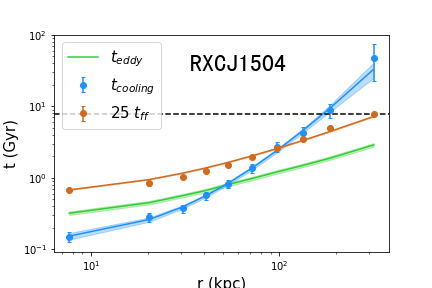
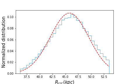
Figure 2: Profiles of $t_{\rm eddy}$, $t_{\rm cool}$ and $25\times t_{\rm ff}$ as a function of the physical radius for RXCJ1504 (top panel). Distribution of intersection radii defined by the condition $t_{\rm cool}(R_{\rm cc})=t_{\rm eddy}(R_{\rm cc})$, obtained by sampling random profiles extracted according to the uncertainty on the best-fit profile (tottom panel). The red dashed line shows the Gaussian fit to the distribution used to derive the central value for $R_{\rm ccc}$ and its 1$\sigma$ uncertainty.

7 Results

The profiles of the timescales, $t_{\rm cool}$, $t_{\rm eddy}$, and $t_{\rm ff}$ were obtained by plugging the temperature, density, and mass 3D profiles into Equation 4, 5, and 7. The timescale profiles are shown in Appendix B for all the clusters in our sample. We note that $t_{\rm ff}$ profiles can be fairly approximated with a power law, while $t_{\rm cool}$ profiles show more significant changes in slope. We remark that $t_{\rm cool}$ is very steep in the presence of a strong cool core (with temperature dropping and density increasing toward the center), while it flattens when the core is less prominent. In some cases, $t_{\rm cool}$ has a slight increase toward the center. We notice that in some cases this is associated with the presence of a central AGN and we conclude that this effect may be uniquely due to the combination of AGN wings that have not been properly removed and of the size of the spatial bin that tend to smooth the central density peak. Since this does not affect our measurements of $R_{\rm ccc}$ and $R_{\rm qcf}$, we do not further comment on the shape of $t_{\rm cool}$ and $t_{\rm ff}$ with regard to the initial few spatial bins.

We also note that in a few systems (A1991, PKS0745, RXCJ1504, CL2089, and A1835) we see TI ratios that drop significantly below 10, usually near values of 7-8. This appear to be in contradiction with previous works, where profiles have never observed below the threshold $t_{\rm cool}/t_{\rm ff}=10$ (see Figure 7 of Hogan et al. 2017). While the majority of clusters show a minimum value of the TI-ratio in the 10-40 range, we verify that in all the cases where the profile drops below 10 our results are robust and can be ascribed to our updated analysis and calibration methods. Indeed, we recall that hydrodynamical simulations of self-regulated feeding and feedback in clusters do show the TI ratio falling to 5-10 during major CCA triggering periods (e.g., see Figure 3 in Gaspari et al. 2012b). We argue that as samples expand and become deeper, we expect to identify several more systems to fill such regions where the TI-ratio falls shortly below 10.

Once we fitted the timescale profiles with Polynomial fitting, we compared the best-fit function for $t_{\rm cool}$ with that for $t_{\rm eddy}$ and $t_{\rm ff}$. We estimate $R_{\rm ccc}$ and $R_{\rm qcf}$ at the radii where $t_{\rm cool}$ crosses $t_{\rm eddy}$ and $25\,t_{\rm ff}$, respectively (see Section 2). The best-fit values of $R_{\rm ccc}$ and $R_{\rm qcf}$ and the corresponding errors are computed as follows. We extracted randomly $1000$ profiles according to the statistical uncertainties on the best-fit parameters of each profile. For each cluster, we obtained a distribution of intersection radii $R_{\rm ccc}$ and $R_{\rm qcf}$. Then, we fit the distribution of $R_{\rm ccc}$ and $R_{\rm qcf}$ with a Gaussian, deriving the best-fit value (the center of the Gaussian) and the 1-$\sigma$ uncertainty. An example is given in Figure 2 for the measurement of $R_{\rm ccc}$ in RXCJ1504. Incidentally, we note that some $t_{\rm cool}$ profiles significantly change slopes (see, e.g., 2A0335, Hydra, RXCJ1558, and PKS0745), so that, in principle, we have two intersections. However, the one close to the center is typically associated with a region of the profile with larger uncertainties. When looking at the distribution of intersection radii obtained by considering all the intersections between the randomized time-scale profiles, we fit only the most prominent peak, so that we naturally discarded these few potentially ambiguous cases where a secondary peak is present. We visually checked that there were no cases where two peaks of comparable significance are present in the distribution of intersection radii.

In some other cases, the best fit profiles do not overlap. Nevertheless, the same procedure allows us to obtain an upper limit at a given confidence level. We set the 1-$\sigma$ upper limit to $R_{\rm ccc}$ and $R_{\rm qcf}$, measuring the value below which we find the 84% of the of the measured values. The best fit values for $R_{\rm ccc}$ and $R_{\rm qcf}$, together with the core-excised, emission weighted temperature (for $r>40$ kpc) and total mass with $r_{500}$, are listed in Table 2.

Table 2: Results of our analysis for all the clusters in our sample. Column 1: Cluster name; column 2: Value of $r_{500}$; column 3: Core-excised temperature (for $r>40$ kpc and $r<r_{500}$); column 4: Total mass within R₅₀₀; column 5: Value of $\sigma_{v}$ calculated from Equation 9; column 6: Cool-core condensation radius defined by the condition $t_{\rm cool}(R_{\rm ccc})/t_{\rm eddy}(R_{\rm ccc})=1$ ; column 7: Quenched cooling flow radius defined by the condition $t_{\rm cool}(R_{\rm qcf})/[25\,t_{\rm ff}(R_{\rm qcf})]=1$.; columns 8 and 9: $R_{\rm ccc}$ and $R_{\rm qcf}$ in units of $10^{-2}\times r_{500}$; column 10: Reference of $\sigma_{v}$ measurements to each cluster. where (a) is Gaspari et al. (2018), (b) is Olivares et al. (2019), and (c) is this work using Equation 9.

Cluster	$r_{500}$	T	$M_{500}$	$\sigma_{v}$	$R_{\rm ccc}$	$R_{\rm qcf}$	$R_{\rm ccc}$	$R_{\rm qcf}$	ref
	(kpc)	(keV)	$(10^{14}M_{\odot})$	(km/s)	(kpc)	(kpc)	$(10^{-2}\,r_{500})$	$(10^{-2}\,r_{500})$
A2199	1087	$4.75_{-0.27}^{+0.28}$	$3.8_{-0.3}^{+0.3}$	$216.5_{-6.9}^{+6.9}$	$3.0_{-0.0}^{+0.4}$	$23.0_{-1.3}^{+1.4}$	$0.3_{-0.0}^{+0.0}$	$2.1_{-0.1}^{+0.1}$	(a)
A496	1218	$5.90_{-0.53}^{+0.62}$	$5.4_{-0.7}^{+0.8}$	$326.6_{-89.2}^{+89.2}$	$\leq 10.0$	$23.6_{-0.6}^{+0.8}$	$\leq 0.8$	$1.9_{-0.1}^{+0.1}$	(c)
2A0335	1042	$4.41_{-0.27}^{+0.29}$	$3.4_{-0.3}^{+0.3}$	$316.0_{-6.9}^{+6.9}$	$26.8_{-0.8}^{+0.7}$	$48.4_{-0.8}^{+0.8}$	$2.6_{-0.1}^{+0.1}$	$4.6_{-0.1}^{+0.1}$	(b)
A2589	997	$4.07_{-0.30}^{+0.42}$	$3.0_{-0.3}^{+0.5}$	$297.1_{-81.1}^{+81.1}$	$\leq 15$	$\leq 15$	$\leq 1.5$	$\leq 1.5$	(c)
MKW3S	896	$3.33_{-0.20}^{+0.22}$	$2.2_{-0.2}^{+0.2}$	$284.8_{-77.7}^{+77.7}$	$\leq 10$	$\leq 10$	$\leq 1.1$	$\leq 1.1$	(c)
Hydra	955	$3.79_{-0.18}^{+0.18}$	$2.6_{-0.2}^{+0.2}$	$382.8_{-5.2}^{+5.2}$	$11.0$	$43.8_{-0.9}^{+0.8}$	$\leq 1.2$	$4.6_{-0.1}^{+0.1}$	(a)
A85	1124	$5.16_{-0.22}^{+0.24}$	$4.3_{-0.3}^{+0.3}$	$258.1_{-6.9}^{+6.9}$	$7.1_{-0.9}^{+0.9}$	$28.1_{-2.3}^{+1.9}$	$0.6_{-0.1}^{+0.1}$	$2.5_{-0.2}^{+0.2}$	(a)
A2626	875	$3.21_{-0.17}^{+0.17}$	$2.0_{-0.2}^{+0.2}$	$277.7_{-75.8}^{+75.8}$	$\leq 10$	$\leq 20$	$\leq 1.1$	$\leq 2.3$	(c)
A133	1014	$4.25_{-0.23}^{+0.26}$	$3.2_{-0.3}^{+0.3}$	$211.3_{-3.5}^{+3.5}$	$10.0_{-2.4}^{+1.2}$	$32.5_{-1.5}^{+1.3}$	$1.0_{-0.2}^{+0.1}$	$3.2_{-0.1}^{+0.1}$	(a)
SERSIC159	788	$2.64_{-0.12}^{+0.13}$	$1.5_{-0.1}^{+0.1}$	$277.1_{-3.5}^{+3.5}$	$14.5_{-1.1}^{+1.5}$	$74.4_{-2.3}^{+2.9}$	$1.8_{-0.1}^{+0.2}$	$9.4_{-0.3}^{+0.4}$	(a)
A1991	753	$2.43_{-0.14}^{+0.13}$	$1.3_{-0.1}^{+0.1}$	$188.8_{-6.9}^{+6.9}$	$31.0_{-1.1}^{+1.2}$	$38.8_{-1.1}^{+1.2}$	$4.1_{-0.2}^{+0.2}$	$5.1_{-0.1}^{+0.2}$	(a)
A3112	1060	$4.70_{-0.33}^{+0.37}$	$3.7_{-0.4}^{+0.4}$	$446.9_{-5.2}^{+5.2}$	$5.0_{-0.0}^{+0.0}$	$32.7_{-3.2}^{+3.1}$	$0.5_{-0.0}^{+0.0}$	$3.1_{-0.3}^{+0.3}$	(a)
A2029	1441	$8.42_{-0.39}^{+0.41}$	$9.2_{-0.6}^{+0.7}$	$365.9_{-99.9}^{+99.9}$	$5.0_{-0.0}^{+0.0}$	$23.4_{-1.6}^{+1.5}$	$0.3_{-0.0}^{+0.0}$	$1.6_{-0.1}^{+0.1}$	(c)
A2597	948	$3.83_{-0.19}^{+0.20}$	$2.6_{-0.2}^{+0.2}$	$417.4_{-1.7}^{+1.7}$	$10.6_{-1.3}^{+1.1}$	$64.2_{-1.6}^{+1.5}$	$1.1_{-0.1}^{+0.1}$	$6.8_{-0.2}^{+0.2}$	(a)
A3921	1134	$5.42_{-0.41}^{+0.48}$	$4.6_{-0.5}^{+0.6}$	$331.2_{-90.4}^{+90.4}$	$\leq 30$	$\leq 30$	$\leq 2.6$	$\leq 2.6$	(c)
A2244	1149	$5.57_{-0.34}^{+0.42}$	$4.7_{-0.4}^{+0.5}$	$329.6_{-90.0}^{+90.0}$	$\leq 10$	$\leq 100$	$\leq 0.9$	$\leq 8.7$	(c)
RXCJ1558.3	1088	$5.02_{-0.28}^{+0.33}$	$4.0_{-0.3}^{+0.4}$	$239.0_{-5.2}^{+5.2}$	$\leq 30.0$	$62.0_{-2.7}^{+2.6}$	$\leq 2.8$	$5.7_{-0.2}^{+0.2}$	(a)
PKS0745	1742	$12.34_{-1.07}^{+1.30}$	$16.6_{-2.2}^{+2.6}$	$339.0_{-5.2}^{+5.2}$	$12.5_{-1.0}^{+1.1}$	$55.2_{-0.7}^{+0.7}$	$0.7_{-0.1}^{+0.1}$	$3.2_{-0.0}^{+0.0}$	(a)
RXCJ1524.2	1058	$4.79_{-0.28}^{+0.31}$	$3.7_{-0.3}^{+0.4}$	$332.5_{-5.2}^{+5.2}$	$18.4_{-2.6}^{+1.9}$	$42.9_{-1.2}^{+1.3}$	$1.7_{-0.2}^{+0.2}$	$4.1_{-0.1}^{+0.1}$	(b)
RXCJ0352.9	825	$3.00_{-0.14}^{+0.15}$	$1.8_{-0.1}^{+0.1}$	$329.1_{-5.2}^{+5.2}$	$39.5_{-2.0}^{+1.8}$	$58.1_{-1.5}^{+1.9}$	$4.8_{-0.2}^{+0.2}$	$7.0_{-0.2}^{+0.2}$	(a)
A1664	877	$3.43_{-0.16}^{+0.16}$	$2.2_{-0.2}^{+0.2}$	$279.0_{-76.2}^{+76.2}$	$31.0_{-4.3}^{+4.0}$	$75.1_{-2.1}^{+2.6}$	$3.5_{-0.5}^{+0.5}$	$8.6_{-0.2}^{+0.3}$	(c)
A2204	1531	$10.09_{-0.93}^{+1.18}$	$11.8_{-1.6}^{+2.1}$	$382.1_{-104.3}^{+104.3}$	$29.6_{-0.9}^{+0.9}$	$65.7_{-1.3}^{+1.5}$	$1.9_{-0.1}^{+0.1}$	$4.3_{-0.1}^{+0.1}$	(c)
A907	1076	$5.17_{-0.33}^{+0.38}$	$4.1_{-0.4}^{+0.4}$	$323.0_{-88.2}^{+88.2}$	$10.0_{-0.8}^{+0.0}$	$36.5_{-6.6}^{+5.8}$	$0.9_{-0.1}^{+0.0}$	$3.4_{-0.6}^{+0.5}$	(c)
HerculesA	998	$4.49_{-0.27}^{+0.30}$	$3.3_{-0.3}^{+0.3}$	$293.8_{-80.2}^{+80.2}$	$9.6_{-3.6}^{+2.4}$	$43.1_{-7.9}^{+7.7}$	$1.0_{-0.4}^{+0.2}$	$4.3_{-0.8}^{+0.8}$	(c)
RXJ2014.8	1250	$6.92_{-0.45}^{+0.67}$	$6.5_{-0.6}^{+0.9}$	$356.8_{-5.2}^{+5.2}$	$18.5_{-2.1}^{+2.0}$	$58.6_{-2.9}^{+3.5}$	$1.5_{-0.2}^{+0.2}$	$4.7_{-0.2}^{+0.3}$	(a)
A1204	846	$3.33_{-0.18}^{+0.17}$	$2.0_{-0.2}^{+0.2}$	$382.8_{-5.2}^{+5.2}$	$24.4_{-3.3}^{+5.6}$	$99.0_{-6.6}^{+7.6}$	$2.9_{-0.4}^{+0.7}$	$11.7_{-0.8}^{+0.9}$	(a)
Zw2701	1020	$4.94_{-0.25}^{+0.25}$	$3.7_{-0.3}^{+0.3}$	$312.3_{-85.3}^{+85.3}$	$\leq 10.0$	$73.3_{-4.1}^{+5.2}$	$\leq 1.0$	$7.2_{-0.4}^{+0.5}$	(c)
RXCJ1504	1191	$6.63_{-0.50}^{+0.56}$	$5.9_{-0.7}^{+0.7}$	$346.3_{-94.5}^{+94.5}$	$46.1_{-2.6}^{+2.6}$	$103.3_{-4.7}^{+4.8}$	$3.9_{-0.2}^{+0.2}$	$8.7_{-0.4}^{+0.4}$	(c)
RXCJ1459.4	1031	$5.15_{-0.28}^{+0.32}$	$3.9_{-0.3}^{+0.4}$	$307.3_{-83.9}^{+83.9}$	$40.0_{-4.8}^{+1.4}$	$84.0_{-2.6}^{+3.1}$	$3.9_{-0.5}^{+0.1}$	$8.1_{-0.2}^{+0.3}$	(c)
4C+55.16	997	$4.85_{-0.25}^{+0.26}$	$3.6_{-0.3}^{+0.3}$	$306.5_{-83.7}^{+83.7}$	$14.9_{-2.2}^{+2.8}$	$73.8_{-3.6}^{+4.4}$	$1.5_{-0.2}^{+0.3}$	$7.4_{-0.4}^{+0.4}$	(c)
CL2089	881	$3.86_{-0.19}^{+0.19}$	$2.5_{-0.2}^{+0.2}$	$289.3_{-79.0}^{+79.0}$	$45.0_{-2.5}^{+2.9}$	$77.9_{-2.4}^{+3.0}$	$5.1_{-0.3}^{+0.3}$	$8.8_{-0.3}^{+0.3}$	(c)
RXJ2129.6	1148	$6.39_{-0.46}^{+0.52}$	$5.5_{-0.6}^{+0.7}$	$197.4_{-5.2}^{+5.2}$	$21.7_{-5.2}^{+10.7}$	$95.2_{-8.8}^{+12.3}$	$1.9_{-0.5}^{+0.9}$	$8.3_{-0.8}^{+1.1}$	(a)
A1835	1274	$7.81_{-0.57}^{+0.68}$	$7.5_{-0.8}^{+1.0}$	$358.3_{-97.8}^{+97.8}$	$37.5_{-1.7}^{+1.6}$	$87.8_{-1.8}^{+2.3}$	$2.9_{-0.1}^{+0.1}$	$6.9_{-0.1}^{+0.2}$	(c)
RXCJ1023.8	998	$4.91_{-0.32}^{+0.37}$	$3.6_{-0.4}^{+0.4}$	$316.9_{-86.5}^{+86.5}$	$25.0_{-0.0}^{+2.2}$	$109.5_{-5.5}^{+6.3}$	$2.5_{-0.0}^{+0.2}$	$11.0_{-0.6}^{+0.6}$	(c)
CL0348	799	$3.23_{-0.13}^{+0.15}$	$1.9_{-0.1}^{+0.1}$	$273.6_{-74.7}^{+74.7}$	$53.2_{-2.9}^{+2.8}$	$97.9_{-3.6}^{+4.9}$	$6.7_{-0.4}^{+0.3}$	$12.2_{-0.4}^{+0.6}$	(c)
MS1455.0	1014	$5.09_{-0.25}^{+0.27}$	$3.8_{-0.3}^{+0.3}$	$316.5_{-86.4}^{+86.4}$	$32.5_{-5.1}^{+3.9}$	$110.9_{-3.6}^{+3.5}$	$3.2_{-0.5}^{+0.4}$	$10.9_{-0.4}^{+0.3}$	(c)
ZW3146	1187	$7.09_{-0.54}^{+0.57}$	$6.3_{-0.7}^{+0.8}$	$345.0_{-94.2}^{+94.2}$	$32.8_{-2.7}^{+2.6}$	$123.8_{-6.2}^{+7.5}$	$2.8_{-0.2}^{+0.2}$	$10.4_{-0.5}^{+0.6}$	(c)

The distributions of $R_{\rm ccc}$ and $R_{\rm qcf}$ in our sample are shown in Figure 3. To obtain the distributions of $R_{\rm qcf}$ and $R_{\rm ccc}$, first we resampled the $R_{\rm ccc}$ and $R_{\rm qcf}$ values of each cluster 1000 times by randomly varying the profiles of $t_{\rm cool}$, $t_{\rm eddy}$, and $t_{\rm ff}$ according to their uncertainty. Eventually, we averaged the number of values falling in each bin and obtained the final histogram distributions of $R_{\rm qcf}$ and $R_{\rm ccc}$ that properly take into account the uncertainties in the timescale profiles.

We find that the distribution of $R_{\rm ccc}$ is peaked at $\sim 0.01\,r_{500}$, and is entirely included within $\sim 0.07\,r_{500}$. We also notice an apparent bimodality in the distribution of $R_{\rm qcf}$, which is peaked at $\sim 0.04\,r_{500}$, and shows a second peak at $0.07\,r_{500}$. In principle the bimodality in the distribution of $R_{\rm qcf}$ is expected to be significant, since it is visible after the randomization of the $R_{\rm qcf}$ values which would have erased the dip at $\sim 0.05\,r_{500}$ – as this was only due do discreteness effects. However, as we show in the lower panel of Figure 3, the bimodality disappear when the distribution is plotted as a function of the physical radius. Therefore, we do not investigate further this feature. In addition, we recall that, since our sample selection is biased towards cool-core clusters, some features in the distribution of $R_{\rm ccc}$ and $R_{\rm qcf}$ in our sample should not be ascribed to general properties of the cluster population. Finally, we note that the distribution of $R_{\rm ccc}$ is shifted at lower values by a factor of $\sim 3$ with respect to the distribution of $R_{\rm qcf}$.

We note that, historically, the classic cooling radius is often defined as the radius, where $t_{\rm cool}=t_{\rm age}$, and $t_{\rm age}$ is a typical ”age” of the object, roughly estimated as $t(z_{o})-t(z\sim 2)\sim 1/H_{0}$, $t$ is the age of the universe at different redshifts $z$ and $z\sim 2$ is assumed to mark the epoch of galaxy cluster formation. Another arbitrary definition of cooling radius is obtained by directly comparing the cooling time to some absolute reference timescale, for instance, 1 Gyr, or a specific value such as 7.7 Gyr (Hudson et al. 2010). These criteria allow one to derive a simple and immediate order-of-magnitude estimate of the actual cooling radius, at variance with our definition based on a local, physical criterion, independent from the cosmic epoch. Therefore, we will refer to the ”classical” cool-core definition adopting the fixed threshold $t_{\rm cool}<7.7$ Gyr as the radius $R_{7.7}$, and compare it to the physically motivated values of $R_{\rm ccc}$ and $R_{\rm qcf}$. The ”classical” cool-core $R_{7.7}$ distribution is shifted to larger values with respect to $R_{\rm ccc}$ and $R_{\rm qcf}$, distributed in the broad range of $0.1-0.2\,r_{500}$, as shown in Figure 3. Despite the wide distribution, $R_{7.7}$ is clearly disconnected from the physically motivated values for $R_{\rm ccc}$ and $R_{\rm qcf}$. We argue that these values describe more accurately the condensation and the intermittent cooling flow-regions, as we further discuss in the next section (Section 8).

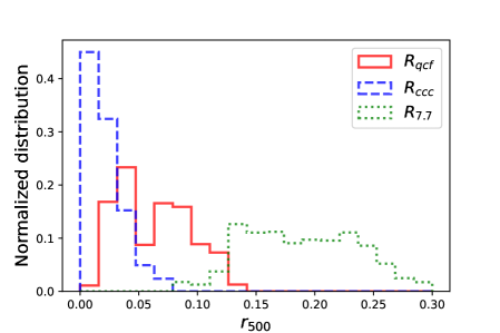
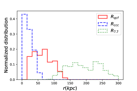
Figure 3: Histogram of the novel cool-core radii $R_{\rm ccc}$ and $R_{\rm qcf}$, compared with the classical cool-core radius (within which $t_{\rm cool}<7.7$ Gyr), as fractions of $r_{500}$ (top) and in kpc unit (bottom).

In Figure 4, we investigate in more details the relation between $R_{\rm qcf}$ and $R_{\rm ccc}$. We can directly verify that $R_{\rm qcf}>R_{\rm ccc}$ for all the clusters, as expected, with a few cases for which $R_{\rm qcf}\sim R_{\rm ccc}$ within the errors. With the bootstrap fitting method, and using the relation:

$${\rm log}\,R_{\rm qcf}=A\times{\rm log}\,R_{\rm ccc}+\gamma,$$ (17)

we obtain $A=0.46^{+0.02}_{-0.03}$ and $\gamma=-0.41^{+0.04}_{-0.05}$. We included also the upper limits in this analysis, shown with arrows in Figure  4. The correlation is statistically very significant, but also shows a considerable intrinsic scatter in addition to the statistical noise. The interesting result is that the relation is significantly different from a linear relation, $R_{\rm qcf}\propto R_{\rm ccc}$. From this, we conclude that larger quenched cool cores have a larger probability to host a larger cool-core condensation region, implying more vigorous precipitation events. In other words, if we assume that a large cool core ($R_{\rm qcf}\sim 0.1\,r_{500}$) is the signature of a cooling and feedback activity ongoing for a long time, we may expect that the precipitation condition (and therefore the condensation region) is extended to the entire cool-core region ($R_{\rm ccc}\sim R_{\rm qcf}$), while in smaller cool cores, the condensation region is progressively smaller (we discuss this further in Section 8).

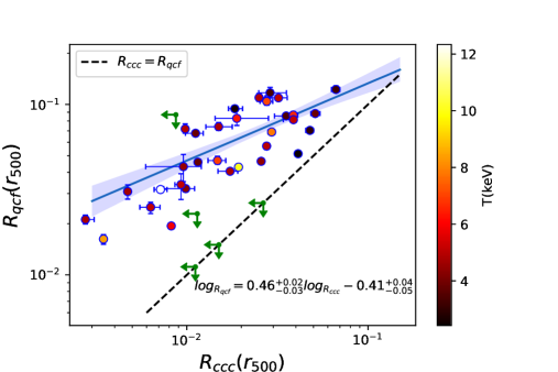
Figure 4: Quenched cooling flow radius $R_{\rm qcf}$ plotted against the cool-core condensation radius $R_{\rm ccc}$, including the upper limits in $R_{\rm qcf}$ and $R_{\rm ccc}$ (green arrows). The solid line is the best-fit power law relation (with 1-$\sigma$ uncertainty shown by the shaded area), while the dashed line shows $R_{\rm qcf}\propto R_{\rm ccc}$ with arbitrary normalization. The color of each point is color coded according to the temperature of each cluster. Error bars correspond to 1-$\sigma$ confidence level.

In Figure 5, we plot the normalized (left panel) and physical (right panel) quenched cool-core radius, $R_{\rm qcf}$, and cool-core condenstation radius, $R_{\rm ccc}$, versus the total mass. The plots show a substantial scatter with no clear dependence on the mass over the range spanned by our sample, except for a small hint of lower values at larger masses (relatively to $r_{\rm 500}$, but not as absolute values). The large intrinsic scatter may reflect the different history of each cluster, with no clear dependence on the total mass (the integrated accretion history) but, rather, on the occurrence of recent major mergers, which have the effect of erasing the cool core and restarting the cooling process and the formation of a new cool core. The smaller $R_{\rm ccc}$ and $R_{\rm qcf}$ values at $M_{500}\sim 10^{15}M_{\odot}$ are affected by small number statistics and probably by a selection bias: smaller cool cores survive the criterion on the net counts within 40 kpc because they are substantially brighter. On the other hand, smaller clusters must have larger cool cores to pass the selection criteria. Extending our sample to the lower mass, galaxy group will be important to understand potential mass trends, which are nevertheless expected to be weak (e.g., Gaspari et al. 2018).

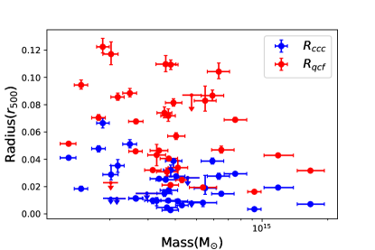
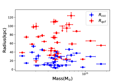
Figure 5: Quenched cool core radius $R_{\rm qcf}$ (red) and cool-core condensation radius $R_{\rm ccc}$ (blue) plotted versus the total mass $M_{500}$. Error bars correspond to 1-$\sigma$ confidence level. In the top (bottom) panel the radii are in units of $r_{500}$ (physical kpc). No dominant trend is observed.

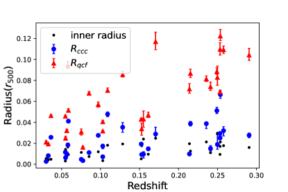
Figure 6: Quenched cooling flow radius $R_{\rm qcf}$ (red) and the cool-core condensation radius $R_{\rm ccc}$ (blue) plotted versus redshift. The black dots show the size of the innermost bins, to visualize of how well we are able to resolve the inner regions compared with the $R_{\rm qcf}$ values.

The dependence of $R_{\rm ccc}$ and $R_{\rm qcf}$ on redshift is shown in Figure 6. In both cases, there is an increasing trend with redshift. We do not attempt to interpret this relation in terms of evolution of the cluster population due to the limited size of our sample and our selection technique.

8 Discussion

Cool cores are one of the most important features of galaxy clusters. As introduced in Section 1, they represent the heart of the ICM atmosphere that fill the galaxy cluster potential well. They roughly demark the reservoir of gas out of which the central SMBH can feed recursively over the cosmic evolution (see the multiscale diagram in the review by Gaspari et al. 2020). However, they are often arbitrarily defined, by comparing the cooling time with ad-hoc timescales such as 1 or 7.7 Gyr (see Hudson et al. 2010 for a detailed discussion). Previous studies also focused on visual definitions, such as the peak in the temperature profile (e.g., Vikhlinin et al. 2006), or classical pure or unheated cooling flow rates (e.g., McDonald et al. 2018). Inspired by the results of Gaspari et al. (2018), we investigated here a more physically-driven way to establish the ”cooling-flow” region, namely, where the ICM plasma actually condenses, subsequently forming multiphase filaments and clouds that rain onto the SMBHs via CCA (e.g., Tremblay et al. 2018; Rose et al. 2019; Juráňová et al. 2019; Olivares et al. 2019, 2022; Temi et al. 2022). As a result of our investigation, we propose that the ratio of crucial ICM feeding and feedback timescales provides a dimensionless and unbiased way to assess such a cooling region, which can potentially differ from the above definition, namely, that of the classical ad hoc ”cool core.” Here, we discuss the implications of our main findings, namely: 1) definition and meaning of the condensation cool-core radius $R_{ccc}$; 2) definition and meaning of the quenched cooling flow radius $R_{qcf}$; 3) $R_{ccc}$-$R_{qcf}$ relation and constraints on the AGN feeding-feedback duty cycle.

8.1 Definition and meaning of th condensation cool-core radius

We find that a more realistic definition for the roughly spherical region where condensation and precipitation are strongly effective, is provided by the condensation cool-core radius $R_{\rm ccc}$. Here, we find typical values $r\sim 0.01<R_{\rm ccc}/r_{500}<0.05$, that is, about 5-10$\times$ smaller than the above classical definitions of the cool core radius (see upper panel of Figure 3). This has been achieved by leveraging the $C$-ratio crossing around unity, which is a simple and clear physical threshold that characterizes the triggering of the turbulent non-linear thermal instability and related top-down multiphase condensation (e.g., Gaspari et al. 2017; Voit 2018; Olivares et al. 2022). In our sample of massive galaxy clusters, $C\sim 1$ yields a distribution of $R_{\rm ccc}$ peaked at $\sim$ 20 kpc (see lower panel of Figure 3), which is comparable to the values found in the upper envelope of the Gaspari et al. (2018) sample (including poor clusters groups as well). It is important to note that such a novel cool-core condensation radius is not an hypothetical region over which a massive pure cooling flow would ensue, but the actual physical region set by the observed balance of feeding and feedback processes. The scattered but rather flat $R_{\rm ccc}-M_{500}$ relation (see Figure 5) suggests that more local properties (such as the BCG mass) may drive the condensation core evolution. We defer this issue to a subsequent study.

8.2 Definition and meaning of the quenched cooling flow radius

We further explored a complementary criterion $t_{\rm cool}/t_{\rm ff}<25$ to trace the region over which a quenched cooling flow may potentially develop from linear TI (Gaspari et al. 2012b; Sharma et al. 2012; Voit et al. 2015a). Despite the phenomenological non-unitary threshold that is still hard to understand in a comprehensive theoretical framework, the related quenched cooling flow radius, $R_{\rm qcf}$, is another valuable indication of the potentially condensing region out of the heated macro cooling flow. Although it is affected by larger fluctuations in the distribution function, ranging from $0.02$ to $0.13R_{500}$ (or from 20 to 130 kpc; see Figure 3), $R_{\rm qcf}$ tends to be on average larger than $R_{\rm ccc}$ by factor up to $\sim$ 3. We thus find that $R_{\rm ccc}$ is the inner part of the condensation region affected by direct turbulent precipitation and CCA, while $R_{\rm qcf}$ represents the more extended ”weather” over which we expect the secular development of a quenched cooling flow. We expect each cluster to be in different weather stages of the self-regulated feeding and feedback cycle, oscillating between extended and more localized condensation rainfalls ($<0.05\,r_{500}$). On the other hand, $R_{\rm qcf}$ only traces the global quenched cooling flow region, up to $\geq 0.1,r_{500}$, which does not necessarily imply actual condensation. Indeed, most nebular emission and warm gas is typically contained within smaller radii, which are comparable to $R_{\rm ccc}$ (e.g., Gaspari et al. 2018). Therefore, in comparison to the quenched cooling flow radius, $R_{\rm qcf}$, $R_{\rm ccc}$ represents a more reliable and stable indicator for the effective cool core in terms of condensed matter, which can be leveraged in simulations and semi-analytical models, as well as in the interpretation of observations.

Incidentally, we also explored an alternative definition of $R_{\rm qcf}$, corresponding to the condition $t_{\rm cool}/t_{\rm ff}=10$. In this case, we find that less than ten clusters would have a well-defined crossing value, while the majority would instead have an undefined value, due to their profiles slowly approaching the condition $t_{\rm cool}/t_{\rm ff}=10$ in the flat part of the profile. We note, however, that the condition $t_{\rm cool}/t_{\rm ff}=10$ must be considered as a lower bound to the $R_{\rm qcf}$ criterion, as we already mentioned. We are aware that the actual threshold is more likely a range of values, rather than a single-value threshold, and that as a consequence, the actual $R_{\rm qcf}$ distribution may be more scattered than that presented in this work. Nevertheless, we argue that an average ratio $t_{\rm cool}$/$t_{\rm ff}\sim 25$ is a reasonable proxy to trace the initial growth of linear thermal instability (TI) in heated cooling flows (see Hogan et al. 2017). Finally, considering a range of values for the threshold, apart from introducing a large scatter, would not change the qualitative aspects of our results.

8.3 $R_{ccc}$-$R_{qcf}$ relation and constraints on the AGN duty cycle

The $R_{\rm qcf}-R_{\rm ccc}$ relation can give us further insight into the AGN feeding-feedback duty cycle. Notably, there is no linear relation between the two condensation radii: they tend to become comparable at large 100 kpc values but non-linearly diverge as they approach smaller sizes (Fig. 4). The divergence of such radii toward smaller scales can be interpreted through the micro and meso precipitation having a more flickering duty cycle than the macro (ensemble) weather. Such a trend is qualitatively consistent with the CCA variability found in high-resolution 3D hydrodynamical simulations (Gaspari et al. 2017), showing that the characteristic power spectral frequency of the rains has a negative slope (flicker noise). Notably, such feature has been probed in other recent cluster surveys and observations (e.g., McDonald et al. 2021; Somboonpanyakul et al. 2021). Extrapolating below the cluster regime, the sublinear slope implies that smaller halos are expected to have a larger $R_{\rm qcf}-R_{\rm ccc}$ separation; indeed, recent multiwavelength constraints suggest that the raining region is substantially more compact in isolated galaxies (Temi et al. 2022) compared with the global cooling flow zone. Furthermore, we suggest that such differences in ”cool-core” size could allow to reconcile better the differences between the cooling rates $\dot{M}_{\rm cool}$ retrieved via imaging out of the classical large cool core with those constrained via spectroscopy, with the latter usually limited within smaller regions similar to $R_{\rm ccc}$ (e.g., Molendi et al. 2016).

To recap, the above combined evidences suggest a global core radii picture based on $R_{\rm ccc}\la R_{\rm qcf}\ll R_{\rm classic}$. As shown in Fig. 3, each cluster has a ”classical” cool-core region $R_{\rm classic}$, which envelopes a sphere with radius up to $\sim 0.2-0.3\,r_{500}$ (or several 100 kpc). However, such $R_{\rm classic}$ is purely based on an arbitrary cosmological threshold $t_{\rm cool}<7.7$ Gyr (Hudson et al. 2010). Within such classical cool core where most of the X-ray radiation is emitted (but the hot gas is not able to actually condense into the lower gas phases) we find the long-term quenched cool core $R_{\rm qcf}$, where feeding and feedback processes balance out secularly, akin to an extended macro weather. Inside such cool core, we find the effective condensation rain and flickering CCA traced via $R_{\rm ccc}$ and directly tied to the nebular emission and warm or cold gas detections.

9 Conclusions

We computed the profiles of the cooling time $t_{\rm cool}(r)$, free-fall time $t_{\rm ff}(r)$, and turbulence cascade timescale $t_{\rm eddy}(r)$ in 37 massive ($2\times 10^{14}<M_{500}<2\times 10^{15}M_{\odot}$) galaxy clusters observed with Chandra with high S/N at $0.03<z<0.29$. The profiles have been obtained from observables entirely derived from X-ray datasets, such as temperature, electron density, and metal abundance profiles. We derive for each cluster a condensation core radius $R_{\rm ccc}$ defined as the radius where $t_{\rm cool}=t_{\rm eddy}$, and a (quenched) cooling flow radius $R_{\rm qcf}$ defined as $t_{\rm cool}=25\times t_{\rm ff}$. We accurately evaluate the statistical uncertainties on these timescales and radii, and explore the distribution of their values across our cluster sample. Our main results are as follows.

• The distribution of the condensation core $R_{\rm ccc}$ peaks at $\sim 0.01-0.02\,r_{500}$ and entirely included within $\sim 0.07\,r_{500}$. The distribution of $R_{\rm qcf}$ is broader and shifted on average to $\sim$ $3\times$ larger values with respect to the $R_{\rm ccc}$ distribution.

• We find no significant correlation between total mass and the two radii $R_{\rm ccc}$ and $R_{\rm qcf}$, with a hint of larger values (relatively to $r_{\rm 500}$, but not as absolute values) toward low masses (below $3\times 10^{14}M_{\odot}$, which shall be further explored with larger samples including galaxy groups. Instead, both and $R_{\rm ccc}$ appear to moderately increase with redshift.

• Supported by theoretical models and high-resolution hydrodynamical simulations of the multiphase condensation rain and CCA (e.g., Gaspari et al. 2017, 2018), we find that $R_{\rm qcf}$ is a tracer of the extended quenched cooling flow or macro weather. The smaller cool-core condensation radius $R_{\rm ccc}$ traces instead the actual inner rain, which also drives CCA feeding episodes onto the SMBH. Both proposed core radii are an order of magnitude smaller than the classical and ad-hoc cool-core definition $R_{7.7\,\rm Gyr}$, where the halo is emitting strong X-ray radiation, but not condensing or inflowing.

• We find that the correlation between $R_{\rm qcf}$ and $R_{\rm ccc}$ is non-linear, diverging at lower values up to a factor of 3 over an order of magnitude in $r_{500}$. This relation between the two scales allows us to infer some features of the duty cycle and related appearance or disappearance of the local cooling flow. Specifically, the slope of the $R_{\rm qcf}-R_{\rm ccc}$ relation is measured to be $0.46^{+0.02}_{-0.03}$, and suggests that the micro CCA rain is flickering on and off in the macro weather, in agreement with hydrodynamical simulations (Gaspari et al. 2017).

As shown above, to describe the fate of the multiscale cooling gas and its interplay with the cluster atmosphere, we need a combination of high spatial resolution and good spectroscopic capabilities. For instance, among the future generation of X-ray instruments, those onboard Athena will play an important role to help in this direction. It is expected to achieve a PSF below 10 arcsec over the entire field of view and an effective area at 1 keV a factor $>$ 5 larger than the current detectors, along with the Wide Field Imager (WFI) providing sensitive wide field imaging and spectroscopy and the X-ray Integral Field Unit (X-IFU) delivering spatially resolved high-resolution X-ray spectroscopy – altogether, these instruments will allow for an unprecedented level of accuracy in mapping the state of the gas within 0.1 $r_{500}$ and cool cores in systems at $T>2$ keV up to a redshift of $\la 0.4$. Further, high angular-resolution X-ray facilities such as Lynx and AXIS are proposing to investigate with subarcsecond resolution over a FoV of 400-500 arcmin² the X-ray sky, improving this capability of a factor $\sim 100$ with respect to Chandra ACIS-I. All such core missions will enable crucial steps forward in the characterization and understanding of the weather in galaxy cluster cores by linking the micro, meso, and macro scales as well as above key condensation processes.

Appendix A Derivation of the deprojected electron density (Equation 12)

When fitting the spectra of the projected annuli, we obtain the projected, emission-weighted temperature and metallicity, as well as the projected normalization of the emission measure, corresponding to the normalization of the spectrum. The normalization parameter $K$ of of the mekal spectrum in Xspec is defined as:

$$K=\frac{10^{-14}}{4\pi D_{A}^{2}(1+z)^{2}}\int n_{e}(r)n_{H}(r){\rm d}V\sim\frac{10^{-14}0.82}{4\pi D_{A}^{2}(1+z)^{2}}\int n_{e}(r)^{2}{\rm d}V,$$ (18)

where 0.82 is the cosmic ratio, $n_{H}/n_{e}$, and $n_{e}(r)$ is the radial density profile of the electron density, which is the quantity we want to derive from the observed (projected) values. In the assumption of spherical symmetry, the differential volume element ${\rm d}V$ corresponding to a projected annulus of finite width, $\Delta s$, depends on the projected radius, $s,$ and on the coordinate $z$ along the line of sight, simply as $dV=2\pi s\Delta sdz$. Since $z=\sqrt{(r^{2}-s^{2})}$, we obtain:

$${\rm d}V=2\pi s\Delta s\frac{r{\rm d}r}{\sqrt{r^{2}-s^{2}}}\,.$$ (19)

If we define the function $f(r)$ as

$$f(r)\equiv\frac{0.82\,10^{-14}}{4D_{A}^{2}(1+z)^{2}}n_{e}^{2}(r)\,,$$ (20)

then we have rewritten $K$ as a function of the projected radius, $s,$ in a compact expression:

$$\frac{K(s)}{s\Delta s}=2\int_{s}^{\infty}\frac{rf(r){\rm d}r}{\sqrt{r^{2}-s^{2}}}\,.$$ (21)

If we apply the Abel transform, we can write:

$$f(r)=-\frac{1}{\pi}\int_{r}^{\infty}\frac{d}{ds}\Big{(}\frac{K(s)}{s\Delta s}\Big{)}\frac{{\rm d}s}{\sqrt{s^{2}-r^{2}}}\,.$$ (22)

This allows us to write the square of the electron density with an expression based on observables. Combining Equations A.3 and A.5, we obtain

$$n_{e}^{2}(r)=-\frac{4\times 10^{14}}{0.82\pi}{D^{2}_{A}(1+z)^{2}}\int_{r}^{\infty}\frac{d}{ds}\Big{(}\frac{K(s)}{s\Delta s}\Big{)}\frac{{\rm d}s}{\sqrt{s^{2}-r^{2}}}\,,$$ (23)

which is the same as Equation 12 given in Section 6.

Appendix B Timescale profiles

In Fig. 1, we show the profiles of the cooling time, $t_{\rm cool}$, turbulence eddy time, $t_{\rm eddy}$, and free-fall time, $t_{\rm ff}$. Each row refers to a cluster following the same order of Table 2. In the left panels, we show the points corresponding to the spatial bins of the spectral fits, with the points obtained from the best-fit deprojected temperature and density profiles for $t_{\rm cool}$ and $t_{\rm ff}$. In addition, we plot the polynomial best fit to the time scale profiles as a continuous line, showing the 1-$\sigma$ uncertainty with a shaded area. In the right column, we show the ratio of the best-fit function of $t_{\rm cool}$, $t_{\rm eddy}$, and $t_{\rm ff}$. In particular, $t_{\rm cool}/t_{\rm ff}$ defines $R_{\rm qcf}$ when $t_{\rm cool}/t_{\rm ff}=25$, while $t_{\rm cool}/t_{\rm eddy}$ defines $R_{\rm ccc}$ when $t_{\rm cool}/t_{\rm eddy}=1$. In Fig. 2, we can see that the results of using Equation 8 and Equation 9 to find $R_{\rm ccc}$ are basically the same, and the error between Equation 9 and the real data is also small, so we use Equation 9 to calculate $R_{\rm qcf}$ for those galaxy clusters without measurement data.

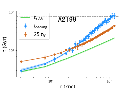
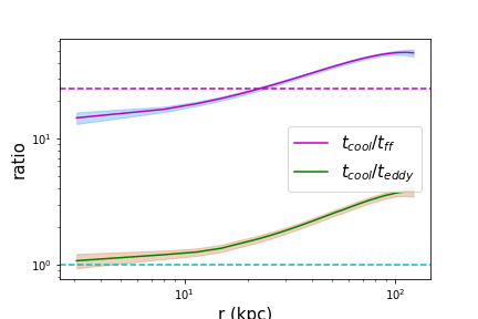
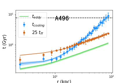
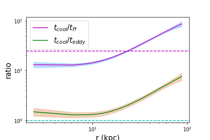
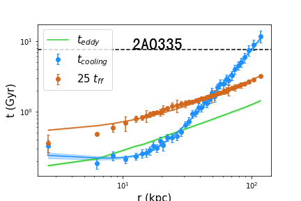
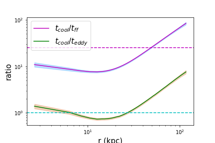
Figure 1: Profiles of the cooling time $t_{\rm cool}$, the turbulence eddy turnover time $t_{\rm eddy}$, and the free fall time $t_{\rm ff}$ (left). Ratio of $t_{\rm cool}/t_{\rm ff}$ that defines $R_{\rm qcf}$, when $t_{\rm cool}/t_{\rm ff}=25$, and $t_{\rm cool}/t_{\rm eddy}$, which defines $R_{\rm ccc}$ when $t_{\rm cool}/t_{\rm eddy}=1$ (right).

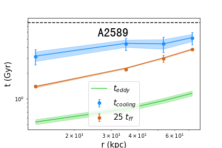
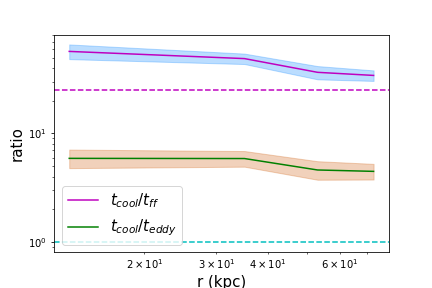
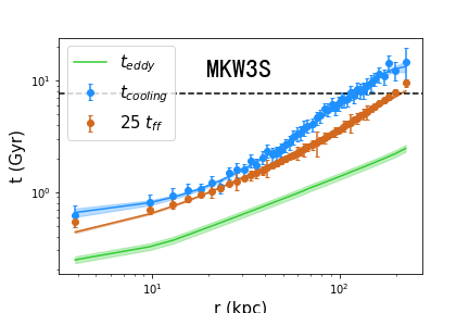
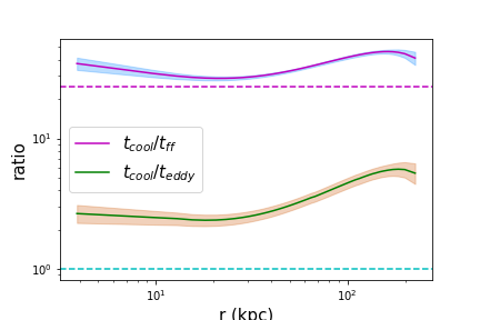
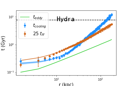
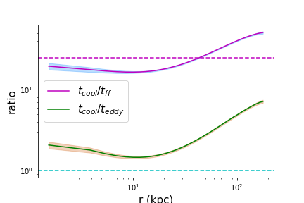
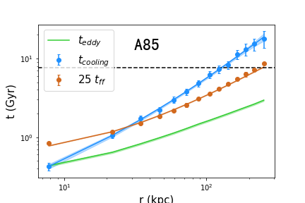
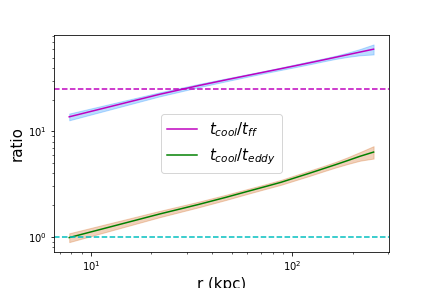
Figure 1: - continued .

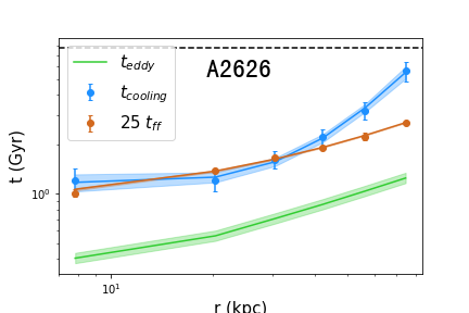
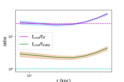
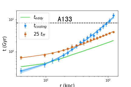
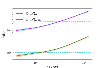
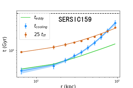
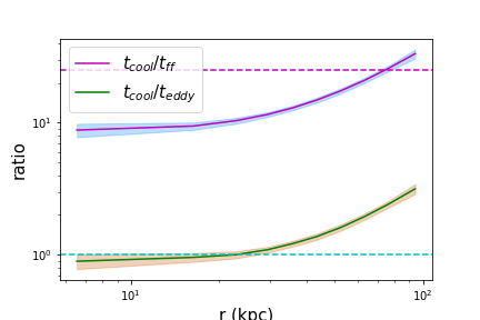
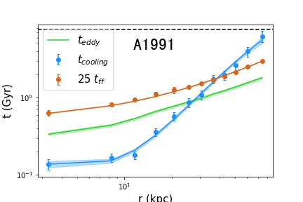
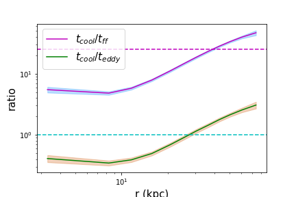
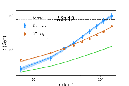
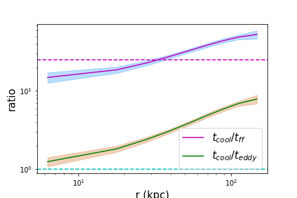
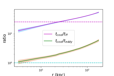
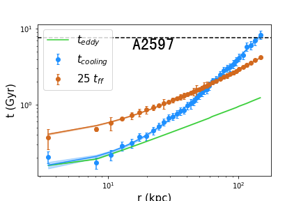
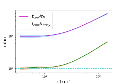
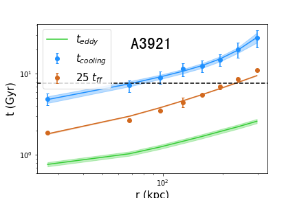
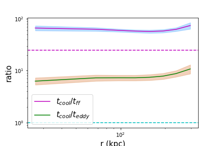
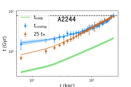
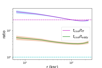
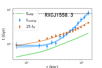
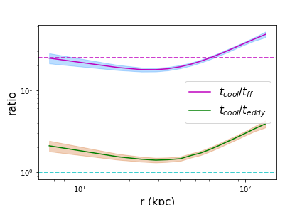
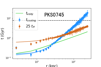
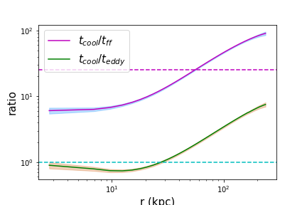
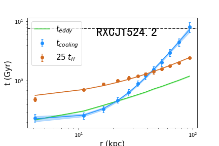
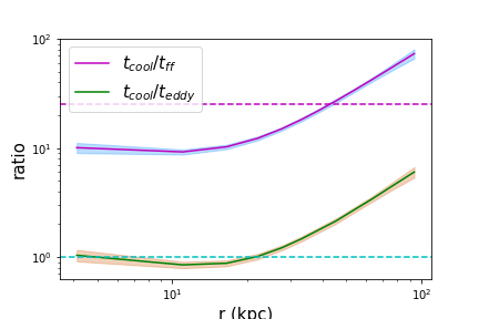
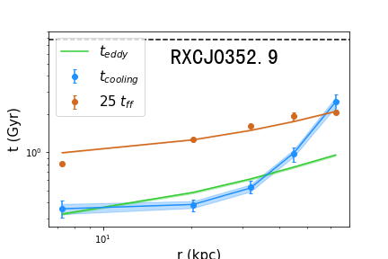
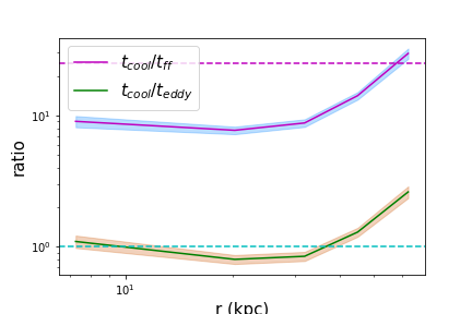
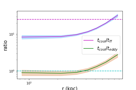
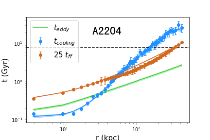
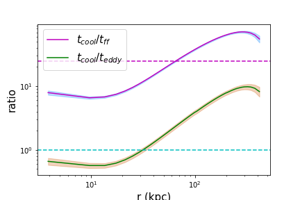
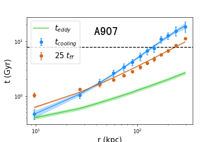
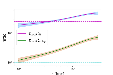
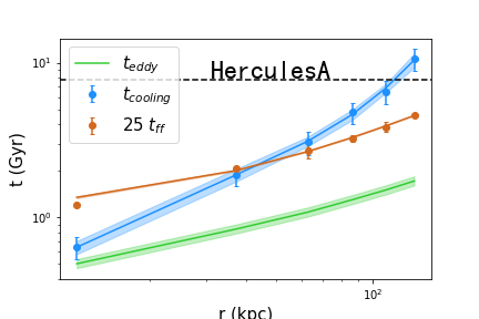
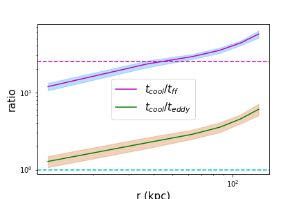
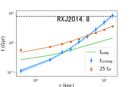
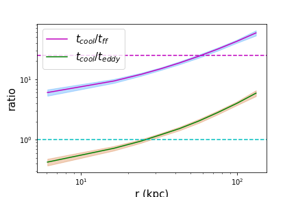
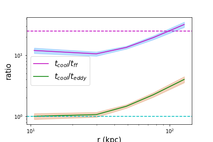
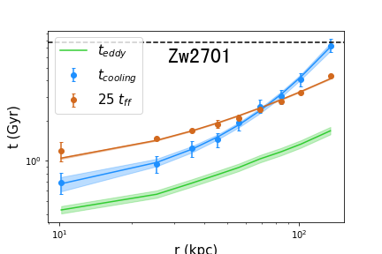
Figure 1: - continued .

Figure 1: - continued .

Figure 1: - continued .

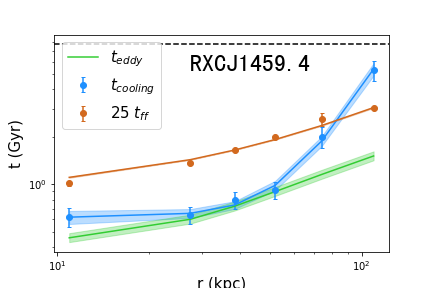
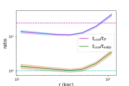
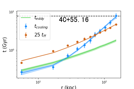
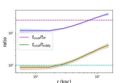
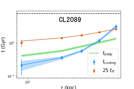
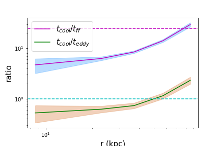
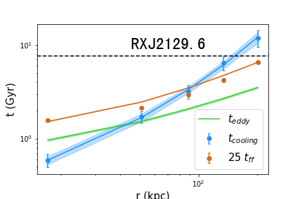
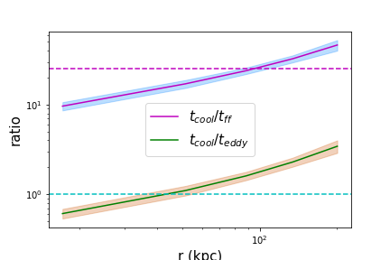
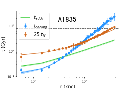
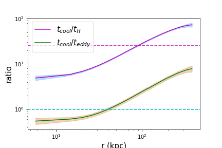
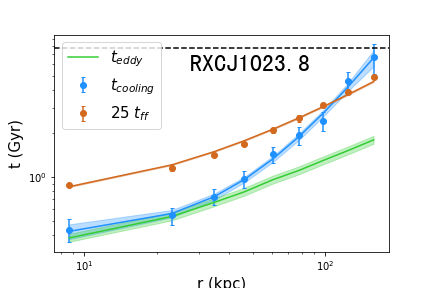
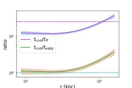
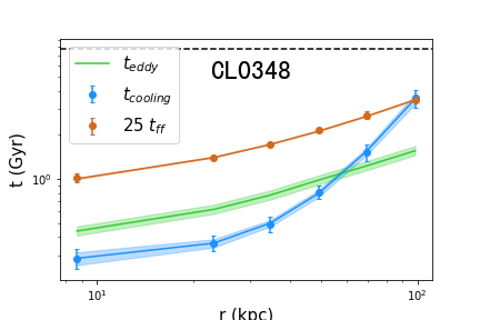
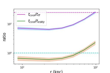
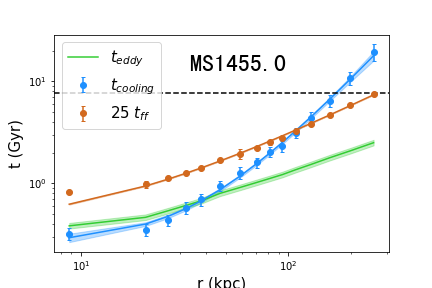
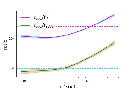
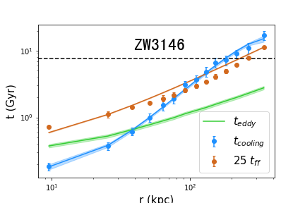
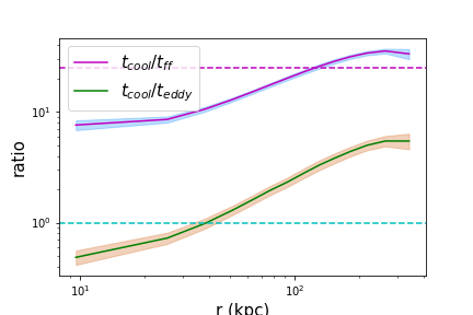
Figure 1: - continued .

Figure 1: - continued .

Figure 1: - continued .

Figure 1: - continued .

Figure 1: - continued .

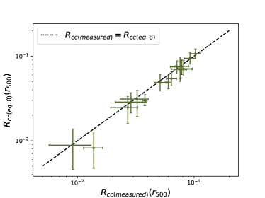
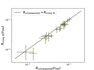
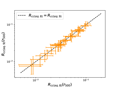
Figure 2: Comparison chart of the results(16 galaxy clusters) of calculating $R_{\rm ccc}$ with Equation 8 and measured data (left). Comparison chart of the results(16 galaxy clusters)of calculating $R_{\rm ccc}$ with Equation 9 and measured data (right). Comparison chart of the results of calculating $R_{\rm ccc}$ with Equations 8 and 9 (bottom).

References

- Arnaud (1996) Arnaud, K. A. 1996, in Astronomical Society of the Pacific Conference Series, Vol. 101, Astronomical Data Analysis Software and Systems V, ed. G. H. Jacoby & J. Barnes, 17
- Asplund et al. (2009) Asplund, M., Grevesse, N., Sauval, A. J., & Scott, P. 2009, ARA&A, 47, 481
- Barai et al. (2016) Barai, P., Murante, G., Borgani, S., et al. 2016, MNRAS, 461, 1548
- Binney & Tremaine (1987) Binney, J. & Tremaine, S. 1987, Galactic Dynamics (Princeton Series in Astrophysics)
- Blanton et al. (2010) Blanton, E. L., Clarke, T. E., Sarazin, C. L., Randall, S. W., & McNamara, B. R. 2010, Proceedings of the National Academy of Science, 107, 7174
- Blanton et al. (2011) Blanton, E. L., Randall, S. W., Clarke, T. E., et al. 2011, ApJ, 737, 99
- Burns et al. (2008) Burns, J. O., Hallman, E. J., Gantner, B., Motl, P. M., & Norman, M. L. 2008, ApJ, 675, 1125
- Cavagnolo et al. (2009) Cavagnolo, K. W., Donahue, M., Voit, G. M., & Sun, M. 2009, ApJS, 182, 12
- Cavaliere & Fusco-Femiano (1978) Cavaliere, A. & Fusco-Femiano, R. 1978, A&A, 70, 677
- Chen et al. (2007) Chen, Y., Reiprich, T. H., Böhringer, H., Ikebe, Y., & Zhang, Y. Y. 2007, A&A, 466, 805
- De Grandi et al. (2004) De Grandi, S., Ettori, S., Longhetti, M., & Molendi, S. 2004, A&A, 419, 7
- Dennis & Chandran (2005) Dennis, T. J. & Chandran, B. D. G. 2005, ApJ, 622, 205
- Diehl et al. (2008) Diehl, S., Li, H., Fryer, C. L., & Rafferty, D. 2008, ApJ, 687, 173
- Domainko et al. (2004) Domainko, W., Gitti, M., Schindler, S., & Kapferer, W. 2004, A&A, 425, L21
- Donahue & Voit (2004) Donahue, M. & Voit, G. M. 2004, in Clusters of Galaxies: Probes of Cosmological Structure and Galaxy Evolution, ed. J. S. Mulchaey, A. Dressler, & A. Oemler, 143
- Dunn & Fabian (2006) Dunn, R. J. H. & Fabian, A. C. 2006, MNRAS, 373, 959
- Edge (2001) Edge, A. C. 2001, MNRAS, 328, 762
- Edge & Frayer (2003) Edge, A. C. & Frayer, D. T. 2003, ApJ, 594, L13
- Ehlert et al. (2011) Ehlert, S., Allen, S. W., von der Linden, A., et al. 2011, MNRAS, 411, 1641
- Ettori & Brighenti (2008) Ettori, S. & Brighenti, F. 2008, MNRAS, 387, 631
- Ettori et al. (2002) Ettori, S., De Grandi, S., & Molendi, S. 2002, A&A, 391, 841
- Fabian (1994) Fabian, A. C. 1994, ARA&A, 32, 277
- Fabian & Nulsen (1977) Fabian, A. C. & Nulsen, P. E. J. 1977, MNRAS, 180, 479
- Fabian et al. (2003a) Fabian, A. C., Sanders, J. S., Allen, S. W., et al. 2003a, MNRAS, 344, L43
- Fabian et al. (2003b) Fabian, A. C., Sanders, J. S., Crawford, C. S., et al. 2003b, MNRAS, 344, L48
- Field (1965) Field, G. B. 1965, ApJ, 142, 531
- Gaspari (2015) Gaspari, M. 2015, MNRAS, 451, L60
- Gaspari et al. (2012a) Gaspari, M., Brighenti, F., & Temi, P. 2012a, MNRAS, 424, 190
- Gaspari & Churazov (2013) Gaspari, M. & Churazov, E. 2013, A&A, 559, A78
- Gaspari et al. (2014) Gaspari, M., Churazov, E., Nagai, D., Lau, E. T., & Zhuravleva, I. 2014, A&A, 569, A67
- Gaspari et al. (2019) Gaspari, M., Eckert, D., Ettori, S., et al. 2019, ApJ, 884, 169
- Gaspari et al. (2018) Gaspari, M., McDonald, M., Hamer, S. L., et al. 2018, ApJ, 854, 167
- Gaspari et al. (2012b) Gaspari, M., Ruszkowski, M., & Sharma, P. 2012b, ApJ, 746, 94
- Gaspari & Sa̧dowski (2017) Gaspari, M. & Sa̧dowski, A. 2017, ApJ, 837, 149
- Gaspari et al. (2017) Gaspari, M., Temi, P., & Brighenti, F. 2017, MNRAS, 466, 677
- Gaspari et al. (2020) Gaspari, M., Tombesi, F., & Cappi, M. 2020, Nature Astronomy, 4, 10
- Gonzalez et al. (2013) Gonzalez, A. H., Sivanandam, S., Zabludoff, A. I., & Zaritsky, D. 2013, ApJ, 778, 14
- Guainazzi & Tashiro (2018) Guainazzi, M. & Tashiro, M. S. 2018, arXiv e-prints, arXiv:1807.06903
- Guo & Oh (2008) Guo, F. & Oh, S. P. 2008, MNRAS, 384, 251
- Hitomi Collaboration et al. (2016) Hitomi Collaboration, Aharonian, F., Akamatsu, H., et al. 2016, Nature, 535, 117
- Hlavacek-Larrondo et al. (2015) Hlavacek-Larrondo, J., McDonald, M., Benson, B. A., et al. 2015, ApJ, 805, 35
- Hofmann et al. (2016) Hofmann, F., Sanders, J. S., Nandra, K., Clerc, N., & Gaspari, M. 2016, A&A, 585, A130
- Hogan et al. (2017) Hogan, M. T., McNamara, B. R., Pulido, F. A., et al. 2017, ApJ, 851, 66
- Hudson et al. (2010) Hudson, D. S., Mittal, R., Reiprich, T. H., et al. 2010, A&A, 513, A37
- Iapichino et al. (2010) Iapichino, L., Maier, A., Schmidt, W., & Niemeyer, J. C. 2010, in American Institute of Physics Conference Series, Vol. 1241, American Institute of Physics Conference Series, ed. J.-M. Alimi & A. Fuözfa, 928–934
- Juráňová et al. (2019) Juráňová, A., Werner, N., Gaspari, M., et al. 2019, MNRAS, 484, 2886
- Kaastra et al. (2001) Kaastra, J. S., Ferrigno, C., Tamura, T., et al. 2001, A&A, 365, L99
- Lau et al. (2017) Lau, E. T., Gaspari, M., Nagai, D., & Coppi, P. 2017, ApJ, 849, 54
- Liu et al. (2020) Liu, A., Tozzi, P., Ettori, S., et al. 2020, A&A, 637, A58
- Liu et al. (2015) Liu, A., Yu, H., Tozzi, P., & Zhu, Z.-H. 2015, ApJ, 809, 27
- Maccagni et al. (2021) Maccagni, F. M., Serra, P., Gaspari, M., et al. 2021, A&A, 656, A45
- Makishima et al. (2001) Makishima, K., Ezawa, H., Fukuzawa, Y., et al. 2001, PASJ, 53, 401
- Mathews et al. (2006) Mathews, W. G., Faltenbacher, A., & Brighenti, F. 2006, ApJ, 638, 659
- McDonald et al. (2012) McDonald, M., Bayliss, M., Benson, B. A., et al. 2012, Nature, 488, 349
- McDonald et al. (2018) McDonald, M., Gaspari, M., McNamara, B. R., & Tremblay, G. R. 2018, ApJ, 858, 45
- McDonald et al. (2021) McDonald, M., McNamara, B. R., Calzadilla, M. S., et al. 2021, ApJ, 908, 85
- McDonald et al. (2019) McDonald, M., McNamara, B. R., Voit, G. M., et al. 2019, ApJ, 885, 63
- McKinley et al. (2022) McKinley, B., Tingay, S. J., Gaspari, M., et al. 2022, Nature Astronomy, 6, 109
- McNamara & Nulsen (2007) McNamara, B. R. & Nulsen, P. E. J. 2007, ARA&A, 45, 117
- McNamara et al. (2005) McNamara, B. R., Nulsen, P. E. J., Wise, M. W., et al. 2005, Nature, 433, 45
- McNamara & O’Connell (1989) McNamara, B. R. & O’Connell, R. W. 1989, AJ, 98, 2018
- McNamara et al. (2014) McNamara, B. R., Russell, H. R., Nulsen, P. E. J., et al. 2014, ApJ, 785, 44
- McNamara et al. (2000) McNamara, B. R., Wise, M., Nulsen, P. E. J., et al. 2000, ApJ, 534, L135
- Molendi et al. (2023) Molendi, S., De Grandi, S., Rossetti, M., et al. 2023, A&A, 670, A104
- Molendi & Pizzolato (2001) Molendi, S. & Pizzolato, F. 2001, ApJ, 560, 194
- Molendi et al. (2016) Molendi, S., Tozzi, P., Gaspari, M., et al. 2016, A&A, 595, A123
- North et al. (2021) North, E. V., Davis, T. A., Bureau, M., et al. 2021, MNRAS, 503, 5179
- O’Hara et al. (2006) O’Hara, T. B., Mohr, J. J., Bialek, J. J., & Evrard, A. E. 2006, ApJ, 639, 64
- Olivares et al. (2019) Olivares, V., Salome, P., Combes, F., et al. 2019, A&A, 631, A22
- Olivares et al. (2022) Olivares, V., Salomé, P., Hamer, S. L., et al. 2022, A&A, 666, A94
- Pasini et al. (2021) Pasini, T., Finoguenov, A., Brüggen, M., et al. 2021, MNRAS, 505, 2628
- Peterson & Fabian (2006) Peterson, J. R. & Fabian, A. C. 2006, Phys. Rep, 427, 1
- Peterson et al. (2001) Peterson, J. R., Paerels, F. B. S., Kaastra, J. S., et al. 2001, A&A, 365, L104
- Pinto et al. (2018) Pinto, C., Bambic, C. J., Sanders, J. S., et al. 2018, MNRAS, 480, 4113
- Planck Collaboration et al. (2016) Planck Collaboration, Ade, P. A. R., Aghanim, N., et al. 2016, A&A, 594, A13
- Ponman et al. (1999) Ponman, T. J., Cannon, D. B., & Navarro, J. F. 1999, Nature, 397, 135
- Pratt et al. (2010) Pratt, G. W., Arnaud, M., Piffaretti, R., et al. 2010, A&A, 511, A85
- Rasera et al. (2008) Rasera, Y., Lynch, B., Srivastava, K., & Chandran, B. 2008, ApJ, 689, 825
- Rose et al. (2019) Rose, T., Edge, A. C., Combes, F., et al. 2019, MNRAS, 489, 349
- Russell et al. (2017) Russell, H. R., McDonald, M., McNamara, B. R., et al. 2017, ApJ, 836, 130
- Ruszkowski et al. (2004) Ruszkowski, M., Bruggen, M., & Begelman, M. C. 2004, in American Astronomical Society Meeting Abstracts, Vol. 204, American Astronomical Society Meeting Abstracts #204, 09.01
- Sanders et al. (2010) Sanders, J. S., Fabian, A. C., Smith, R. K., & Peterson, J. R. 2010, MNRAS, 402, L11
- Sanderson et al. (2006) Sanderson, A. J. R., Ponman, T. J., & O’Sullivan, E. 2006, MNRAS, 372, 1496
- Santos et al. (2008) Santos, J. S., Rosati, P., Tozzi, P., et al. 2008, A&A, 483, 35
- Schuecker et al. (2004) Schuecker, P., Finoguenov, A., Miniati, F., Böhringer, H., & Briel, U. G. 2004, A&A, 426, 387
- Sharma et al. (2012) Sharma, P., McCourt, M., Quataert, E., & Parrish, I. J. 2012, MNRAS, 420, 3174
- Shin et al. (2016) Shin, J., Woo, J.-H., & Mulchaey, J. S. 2016, ApJS, 227, 31
- Simionescu et al. (2019) Simionescu, A., ZuHone, J., Zhuravleva, I., et al. 2019, Space Sci. Rev., 215, 24
- Somboonpanyakul et al. (2021) Somboonpanyakul, T., McDonald, M., Gaspari, M., Stalder, B., & Stark, A. A. 2021, ApJ, 910, 60
- Sun (2009) Sun, M. 2009, ApJ, 704, 1586
- Sutherland & Dopita (1993) Sutherland, R. S. & Dopita, M. A. 1993, ApJS, 88, 253
- Tamura et al. (2001) Tamura, T., Kaastra, J. S., Peterson, J. R., et al. 2001, A&A, 365, L87
- Temi et al. (2018) Temi, P., Amblard, A., Gitti, M., et al. 2018, ApJ, 858, 17
- Temi et al. (2022) Temi, P., Gaspari, M., Brighenti, F., et al. 2022, ApJ, 928, 150
- Tozzi et al. (2015) Tozzi, P., Gastaldello, F., Molendi, S., et al. 2015, A&A, 580, A6
- Tozzi & Norman (2001) Tozzi, P. & Norman, C. 2001, ApJ, 546, 63
- Tremblay et al. (2018) Tremblay, G. R., Combes, F., Oonk, J. B. R., et al. 2018, ApJ, 865, 13
- Vantyghem et al. (2014) Vantyghem, A. N., McNamara, B. R., Russell, H. R., et al. 2014, MNRAS, 442, 3192
- Vikhlinin et al. (2006) Vikhlinin, A., Kravtsov, A., Forman, W., et al. 2006, ApJ, 640, 691
- Vikhlinin et al. (2005) Vikhlinin, A., Markevitch, M., Murray, S. S., et al. 2005, ApJ, 628, 655
- Voit (2018) Voit, G. M. 2018, ApJ, 868, 102
- Voit et al. (2015a) Voit, G. M., Bryan, G. L., O’Shea, B. W., & Donahue, M. 2015a, ApJ, 808, L30
- Voit et al. (2015b) Voit, G. M., Donahue, M., Bryan, G. L., & McDonald, M. 2015b, Nature, 519, 203
- Voit et al. (2017) Voit, G. M., Meece, G., Li, Y., et al. 2017, ApJ, 845, 80
- Willingale et al. (2013) Willingale, R., Starling, R. L. C., Beardmore, A. P., Tanvir, N. R., & O’Brien, P. T. 2013, MNRAS, 431, 394
- Wilms et al. (2000) Wilms, J., Allen, A., & McCray, R. 2000, ApJ, 542, 914
- Wittor & Gaspari (2020) Wittor, D. & Gaspari, M. 2020, MNRAS, 498, 4983
- Xue & Wu (2000) Xue, Y.-J. & Wu, X.-P. 2000, MNRAS, 318, 715
- Yang et al. (2019) Yang, H.-Y. K., Gaspari, M., & Marlow, C. 2019, ApJ, 871, 6
- Zakamska & Narayan (2003) Zakamska, N. L. & Narayan, R. 2003, ApJ, 582, 162
- Zhuravleva et al. (2014) Zhuravleva, I., Churazov, E., Schekochihin, A. A., et al. 2014, Nature, 515, 85
- ZuHone et al. (2013) ZuHone, J. A., Markevitch, M., Ruszkowski, M., & Lee, D. 2013, ApJ, 762, 69
- Zuhone & Roediger (2016) Zuhone, J. A. & Roediger, E. 2016, Journal of Plasma Physics, 82, 535820301