A probabilistic reduced basis method for parameter-dependent problems
Abstract
Probabilistic variants of Model Order Reduction (MOR) methods have recently emerged for improving stability and computational performance of classical approaches. In this paper, we propose a probabilistic Reduced Basis Method (RBM) for the approximation of a family of parameter-dependent functions. It relies on a probabilistic greedy algorithm with an error indicator that can be written as an expectation of some parameter-dependent random variable. Practical algorithms relying on Monte Carlo estimates of this error indicator are discussed. In particular, when using Probably Approximately Correct (PAC) bandit algorithm, the resulting procedure is proven to be a weak greedy algorithm with high probability. Intended applications concern the approximation of a parameter-dependent family of functions for which we only have access to (noisy) pointwise evaluations. As a particular application, we consider the approximation of solution manifolds of linear parameter-dependent partial differential equations with a probabilistic interpretation through the Feynman-Kac formula.
Keywords: Reduced basis method, probabilistic greedy algorithm, parameter-dependent partial differential equation, Feynman-Kac formula
2010 AMS Subject Classifications: 65N75, 65D15
1 Introduction
This article focuses on the approximation of a family of functions indexed by a parameter , each function being an element of some high-dimensional vector space .
The functions can be known a priori, or implicitly given through parameter-dependent equations. In multi-query contexts such as optimization, control or uncertainty quantification, one is interested in computing for many instances of the parameter. For complex numerical models, this can be computationally intractable. Model order reduction (MOR) methods aim at providing an approximation of which can be evaluated efficiently for any in the parameter set .
For linear approximation methods, an approximation is obtained by means of a projection onto a low-dimensional subspace which is chosen to approximate at best , uniformly over
for empirical interpolation method (EIM) or reduced basis method (RBM), or in mean-square sense for proper orthogonal decomposition (POD) or proper generalized decomposition (PGD) methods (see, e.g., the survey [26]) .
Probabilistic variants of MOR methods have been recently proposed for improving stability and computational performance of classical MOR methods. In [12], the authors introduced a probabilistic greedy algorithm for the construction of reduced spaces , which uses different training sets in with moderate cardinality, randomly chosen at each iteration, that allows a sparse exploration of a possibly high-dimensional parameter set.
In [11], the authors derive a similar probabilistic EIM using sequential sampling in , which provides an interpolation with a prescribed precision with high probability. Let us also mention that a control variate method using a reduced basis paradigm has been proposed in [9] for Monte Carlo (MC) estimation of the expectation of a collection of random variables in a space of second-order random variables. A greedy algorithm is introduced to select a subspace of random variables, that relies on a statistical estimation of the projection error. This algorithm has been analyzed in [8] and proven to be a weak greedy algorithm with high probability. Probabilistic approaches have also been introduced for providing efficient and numerically stable error estimates for reduced order models [21, 22, 28, 29]. In [1, 3, 2, 27, 31],
random sketching methods have been systematically used in different tasks of projection-based model order reduction, including the construction of reduced spaces or libraries of reduced spaces, the projection onto these spaces, the error estimation and preconditioning.
Here, we consider the problem of computing an approximation of within a reduced basis framework. The reduced basis method performs in two steps, offline and online. During the offline stage, a reduced space is generated from snapshots at parameter values greedily selected by maximizing over (or some subset of ) an error indicator which provides a measure of the discrepancy between and .
Then, during the online step, is obtained by some projection onto .
In this paper, we propose a probabilistic greedy algorithm for which is the square error norm ,
expressed as the expectation of some parameter-dependent random variable ,
| (1) |
For maximizing we rely on MC estimates. We consider either a naive MC approach with fixed number of samples or a PAC (Probably Approximately Correct) bandit algorithm proposed by the authors in [6] based on adaptive sampling. The algorithm only requires a limited number of samples by preferably sampling random variables associated with a probable maximizer . It is particularly suitable for applications
where the random variable is costly to sample.
Under suitable assumptions on the distribution of , it provides a PAC maximizer in relative precision, meaning that with high probability the parameter is a quasi-optimal solution of the optimization problem. We prove in this work that the resulting greedy algorithm is a weak-greedy algorithm with high probability.
Intended applications concern the approximation of a parameter-dependent family of functions defined on a bounded domain for which we have access to (possibly noisy) pointwise evaluations for any . The proposed probabilistic greedy algorithm can be used to generate a sequence of spaces and corresponding interpolations of onto . Assuming and we have a direct access to pointwise evaluations, the square error norm used to select the parameter can be estimated from samples of with a uniform random variable over . It results in a probabilistic EIM in the spirit of [11]. In a fully discrete setting where and are finite sets, can be identified with a matrix and the proposed algorithm is a probabilistic version of adaptive cross approximation for low-rank matrix approximation [4, 30], with a particular column-selection strategy.
Another context is the solution of a linear parameter-dependent partial differential equation (PDE) defined on a bounded domain and whose solution admits a probabilistic representation through the Feynman-Kac formula. This allows to express a pointwise evaluation as the expectation of a functional of some stochastic process. The problem being linear, the error also admits a Feynman-Kac representation, which again allows to express the square error norm as the expectation of some random variable and to estimate it through Monte-Carlo simulations of stochastic processes. This is a natural framework to apply the proposed probabilistic greedy algorithm, which allows a direct estimation of the targeted error norm and avoids the use of possibly highly biased residual based error estimates. This leads to error estimators with better effectivity, which improves the behavior of weak-greedy algorithms. In practice, as the exact solution of the PDE is not available, the snapshots used for generating the reduced space are numerical approximations computed from pointwise evaluations of the exact solution by some interpolation or learning procedure. This results in a fully probabilistic setting which opens the route for the solution of high-dimensional PDEs (see, e.g. [5] where the authors rely on interpolation on sparse polynomial spaces).
This paper is structured as follows. In Section 2 we recall basic facts concerning reduced basis method. Then in Section 3 we present and analyze our new probabilistic greedy algorithm. Based on this algorithm, we derive in Section 4 a new reduced basis method for parameter-dependent PDEs with probabilistic interpretation. Numerical results illustrating the performance of the proposed approaches are presented in Section 5.
2 Reduced basis greedy algorithms
As discussed in the introduction, reduced basis method relies on two steps. We mainly focus on the offline stage during which the reduced subspace is constructed. In particular, we recall in this section some basic facts concerning greedy algorithms usually considered in that context. For detailed overview on that topic see, e.g., surveys [20, 25].
Throughout this paper, is some Hilbert space equipped with a norm . We seek an approximation of in a low-dimensional space which is designed to well approximate the solution manifold
A benchmark for optimal linear approximation is given by the Kolmogorov -width
where the infimum is taken over all -dimensional subspaces of and where stands for the orthogonal projection onto . However, an optimal space is in general out of reach. A prominent approach is to rely on a greedy algorithm for generating a sequence of spaces from suitably selected parameter values. Starting from , the -th step of this algorithm reads as follows. Given and the corresponding subspace
a new parameter value is selected as
| (2) |
where stands for an approximation of in . However, this ideal algorithm is still unfeasible in practice, at least for the two following reasons:
-
1)
computing the error for all may be unfeasible in practice (e.g. when is only given by some parameter-dependent equation), and
-
2)
maximizing this error over is a non trivial optimization problem.
Point 1) is usually tackled by selecting a parameter which maximizes some surrogate error indicator that can be easily estimated. Assuming is a quasi-optimal projection of onto and assuming is equivalent to , there exists such that
| (3) |
which yields a weak-greedy algorithm. Quasi-optimality means that the approximation of in satisfies
| (4) |
for some constant independent from and . Although the generated sequence is not optimal, it has been proven in [7, 10, 15] that the approximation error
has the same type of decay as the benchmark for algebraic or exponential convergence.
Remark 2.1.
In the case of parameter-dependent linear equation arising e.g., from the discretization of some parameter-dependent linear PDE of the form with , the approximation is typically obtained through some (Petrov-)Galerkin projection onto , with a complexity depending on . In such a context, a weak greedy algorithm classically involves a certified residual based error estimate , that is an upper bound of the true error. However, for some applications, such an error estimate can be pessimistic (when the underlying discrete operator is badly conditionned) so that the generated sequence is far from being optimal. A possible strategy to improve such an estimate is to consider a preconditioned residual [13, 31, 2]. In Section 4, we overcome this limitation by considering for the targeted square error norm , which is evaluated using adaptive Monte-Carlo estimations.
Point 2) is addressed by transforming the continuous optimization problem over into a discrete optimization over a finite subset . Choosing the training set is a delicate task.
As pointed out in [12, Section 2], if is an -net
of , then a greedy algorithm for the approximation of the discrete solution manifold generates a sequence of spaces
that are able to achieve a precision in with similar performance as the ideal greedy algorithm.
However, the cardinality of may be very large
for a parameter set in a high-dimensional space and when a low precision is required.
In [12], the authors propose a greedy algorithm which uses different training sets randomly chosen at each step. Under suitable assumptions on the approximability of the solution map by sparse polynomial expansions, training sets can be chosen of moderate size independent of the parametric dimension .
To conclude this section, we give a practical deterministic (weak)-greedy algorithm that can be summarized as follows.
Algorithm 2.2 (Deterministic greedy algorithm).
Let be a discrete training set and .
For proceed as follows.
-
(Step 1.)
Select
-
(Step 2.)
Compute and update .
Usually, Algorithm 2.2 is stopped when is below some target precision or for a given dimension .
3 A probabilistic greedy algorithm
In this section, we motivate and present a probabilistic variant of Algorithm 2.2. Such an algorithm relies on the concept of Probably Approximately Correct (PAC) maximum. It is proven to be a weak greedy algorithm with high probability.
As a starting point for our work, we assume that, for any value in , the error estimator required at each step of Algorithm 2.2 admits the following form
| (5) |
where is some parameter-dependent real valued random variable, defined on the probability space . Here, is a probabilistic representation of the current square error depending on the targeted applications as discussed in what follows.
Example 3.1 (Estimate of the norm of approximation error).
Suppose that belongs to the Lebesgue space of square integrable functions defined on a bounded set . If , then (5) holds with where is a random variable with uniform distribution over .
Example 3.2 (Greedy algorithm for control variate [8, 9]).
Let us suppose that we want to compute an MC estimate of the expectation of a parameter-dependent family of random variables belonging to a Hilbert space of centered second-order random variables. MC estimate is known to slowly converge with respect to the number of samples of . Variance reduction techniques based on control variates are usually used to improve MC estimates. In [8] the authors propose a RB paradigm to compute a control variate with a greedy algorithm of the form of Algorithm 2.2 where with in (5).
3.1 Main algorithm
Solving the following optimization problem
| (6) |
is in general out of reach, since is unknown a priori or too costly to compute. Then, we propose a greedy algorithm with an approximate solution of (6).
Algorithm 3.3 (Probabilistic greedy algorithm).
Let be a discrete training set. Starting from , proceed, for , as follows.
-
(Step 1.)
Select
-
(Step 2.)
Compute and update .
The question is now how to choose properly the set of candidate parameter values ? In view of numerical applications, a first practical and naive approach is to seek maximizing the empirical mean, i.e.
where with i.i.d. copies of .
In the following, this algorithm will be called MC-greedy. Despite its simplicity, it is well known that such an estimate for the expectation suffers from low convergence with respect to the number of samples leading to possible high computational costs especially if is expensive to evaluate. Moreover, nothing ensures that the returned (random) parameter is a (quasi-)optimum for (6), almost surely or at least with high probability.
Instead, the so-called bandit algorithms (see, e.g., monograph [23]) are good candidates to address (6). Here, we particularly focus on PAC bandit algorithms that for each return a parameter value which is a probably approximately correct (PAC) maximum in relative precision for over (see [6]). For a given and probability , letting , such an algorithm returns satisfying
| (7) |
We use the notation when satisfies (7). The resulting greedy algorithm is called PAC-greedy. In practice, the adaptive bandit algorithm in relative precision introduced in [6, Section 3.2] is particularly interesting in the case where is costly to evaluate since it preferentially samples the random variable for the parameter values for which it is more likely to find a maximum. Hence, it outperforms the mean complexity of a naive approach in terms of number of generated samples. Appendix A gives a detailed presentation of such a PAC adaptive bandit algorithm. As stated in Proposition A.3, such an algorithm provides a PAC maximum in relative precision, that fulfills (7), in the particular case where are random variables satisfying some concentration inequality. The interested reader can refer to [6] and included references for more details.
3.2 Analysis of PAC-greedy algorithm
Now, we propose and analyze a probabilistic greedy algorithm where the parameter is a PAC maximum in relative precision for (5) i.e. satisfying (7), at each step .
At a step of the Algorithm 3.3, the reduced space , as well as the approximation are no longer deterministic. Indeed, they are related to the selected parameters depending themselves on the errors at the previous steps through i.i.d. samples of the random variables for all and (required during PAC selection of ). Now, we prove that Algorithm 3.3 is a weak greedy algorithm with high probability.
Theorem 3.4.
Proof.
Let first introduce some useful notation. We denote by the conditional probability measure with respect to that denotes the collection of random variables for all and , where are i.i.d. copies of . The related conditional expectation is . Now, let , each event being defined as
with . Then, at each step of Algorithm 3.3, the parameter is a PAC maximum knowing i.e.
| (9) |
Finally, as is completely determined by all the steps before (i.e. depending only on ), we have
| (10) |
For all , the quasi-optimality condition (4) and probabilistic representation (10) lead to
| (11) |
Moreover, if holds we have for
| (12) |
by definition of . Thus, by combining (11) and (12) we have that implies for all
We now estimate
where the last inequality derives from (9), which concludes the proof. ∎
Remark 3.5.
Theorem 3.4 proves that Algorithm 3.3 is a weak greedy algorithm, with probability , for the approximation of the discrete solution manifold . Thus, the approximation error has the same decay rate as for algebraic or exponential convergence. In the lines of [12], it is possible to consider also a fully probabilistic variant of Algorithm 3.3, in which a training set randomly chosen is used at each step of Algorithm 3.3 instead of . For a particular class of functions that can be approximated by polynomials with a certain algebraic rate, it can be proven that, for suitable chosen size of random training set , the resulting algorithm is a weak greedy algorithm with high probability with respect to the continuous solution manifold .
4 Reduced basis method for parameter-dependent PDEs with probabilistic interpretation
We recall that this work is motivated by the approximation, in a reduced basis framework, of a costly function defined on the spatial domain depending on the parameters lying in .
Here we consider the problem where is the solution of a parameter-dependent PDE with probabilistic interpretation.
Let be an open bounded domain in . For any parameter , we seek the solution of the following boundary value problem,
| (13) |
where , are respectively the boundary condition and source term, and is a linear and elliptic partial differential operator.
Since the exact solution of (13) is not computable in general, it is classical to consider instead an approximation in some finite dimensional space deduced from some numerical discretization of the PDE. Classical RBM applies in that context, relying on some variational principles to provide an approximation of in a reduced space , of small dimension, obtained through greedy algorithm (see Section 2). Here, we overcome such a priori discretization of the PDE and directly address the approximation of the solution of (13). The key idea is to use the so-called Feynman-Kac representation formula that allows to compute pointwise estimates of for any . This particular framework raises the following practical questions. During the offline step, how to choose a computable error estimator required in greedy algorithm and compute the snapshots required for generating the reduced basis and related reduced space ? During the online step, how to compute the approximation ?
To that goal, in this section, a probabilistic RBM using only (noisy) pointwise evaluations is presented. We first recall the Feynman-Kac formula in Section 4.1. In Section 4.2, we detail a probabilistic greedy algorithm for construction of the reduced space in this setting. Finally, in Section 4.3, we discuss possible approaches for computing the approximation .
4.1 Feynman-Kac representation formula for an elliptic PDE
In what follows, denotes a standard -dimensional Brownian motion defined on the probability space endowed with its natural filtration . For the sake of simplicity, the dependence to parameter is omitted in the presentation of the Feynman-Kac formula.
Let us consider the boundary problem (13), where the partial differential operator is given as
| (14) |
It is the infinitesimal generator associated to the parameter-dependent -dimensional diffusion process , adapted to , solution of the following stochastic differential equation (SDE)
| (15) |
where and are the drift and diffusion coefficients, respectively.
Before recalling Feynman-Kac formula, we introduce additional assumptions and notation. Denoting by both euclidean norm on and Frobenius norm on , we first introduce the assumption that and are Lipschitz continuous.
Assumption 4.1.
There exists a constant such that for all we have
| (16) |
Under Assumption 4.1, there exists a unique strong solution to Equation (15) (see e.g. [16, Chapter 5, Theorem 1.1.]).
Denoting , we introduce the following uniform ellipticity assumption.
Assumption 4.2.
There exists such that
As problem (13) is defined on a bounded domain, we define the first exit time of for the process as
| (17) |
Also, we assume some regularity property on the spatial domain and data.
Assumption 4.3.
The domain is an open connected bounded domain of , regular in the sense that it satisfies
Assumption 4.4.
We assume that is continuous on , is Hölder-continuous on .
The following probabilistic representation theorem [16, Chapter 6, Theorem 2.4] holds.
Theorem 4.5 (Feynman-Kac formula).
4.2 Offline step
During the offline step, the probabilistic greedy algorithm presented in Section 3 is considered to construct the reduced space . The keystone of such an algorithm is the probabilistic reinterpretation of the error estimate as in Equation (5). Using the Feynman-Kac representation formula, we show in Section 4.2.1 that it is possible to rewrite the square of the approximation error as an expectation. Then, in Section 4.2.2, we discuss possible strategies for practical implementation of such an algorithm.
4.2.1 Probabilistic error estimate
Let us assume that is a linear approximation of in a given reduced space (e.g., obtained using Algorithm 3.3). We recall that is the unique solution of (13) with the following probabilistic representation
| (19) |
with the parameter-dependent stopped diffusion process solution of (15). In classical RB methods, the error estimate used in Algorithm 2.2 is usually related to some suitable norm of the equation residual. Here, we follow another path by considering the -norm of the current approximation error , i.e.
In what follows, we give a possible probabilistic reinterpretation of this error. Assuming that is regular enough (the regularity being inherited from the snapshots), the error is the unique solution, for all in , of
| (20) |
where and . By Feynman-Kac representation theorem, for all in , is the unique solution of (20) in and satisfies for all
| (21) |
with the stopped diffusion process solution of (15). Then, we have the following probabilistic reinterpretation for .
Theorem 4.6.
Let be uniformly distributed on . Let and be two independent standard d-dimensional Brownian motions defined on and independent of . For any , let and be solutions of (15) with , respectively. Then we have for any in
| (22) |
with and the Lebesgue measure of .
Proof.
We first recall
Since, for any , and are i.i.d. random processes, we have
and
Then by the law of iterated expectation we obtain (22). ∎
Remark 4.7.
Assuming the existence of probabilistic representations for the gradient of and , it would be possible to consider probabilistic interpretation of other norms of the approximation error, such as the -norm. Such probabilistic representations have been derived in simple cases, see e.g. [17, Corollary IV.5.2].
4.2.2 A probabilistic greedy algorithm using pointwise evaluations
For the purpose of numerical applications, we can apply Algorithm 3.3 together with the error estimate (22) for the construction of the reduced space .
Sample computation.
Snapshot computation.
Within Algorithm 3.3, the reduced space corresponds to . However, the snapshots are generally not available since it requires to compute the exact solution of (13) for parameter instances . From Feynman-Kac formula (18), it is possible to compute MC estimates of from independent realizations of the diffusion process starting from (as detailed in Appendix B). Then a global numerical approximation can be computed in some finite dimensional linear space of dimension (potentially much larger than ), e.g., by interpolation or least-square method, from these MC pointwise estimates. To compensate possible slow convergence of MC estimates, one can consider a sequential approach which uses the approximation error at each step as control variate in order to reduce the variance of MC estimates. Such a strategy has been initially proposed in [18, 19] for interpolation, and recently extended for high dimensional problems in [5].
Projection computation.
For given , the approximation in can be computed by interpolation or a least-square projection using MC estimates given by (36), with suitable choice for evaluation points in (e.g., using magic points for interpolation [24], or optimal sampling for least-squares [14]). The resulting complexity of this projection step is only linear in (up to ).
4.3 Online step
Given the reduced space obtained during the offline stage, the approximation is computed, with a complexity depending only on (and not on ), following the procedure described in the projection step of Section 4.2.2.
5 Numerical applications
The aim of this section is twofold. We first illustrate the feasibility of a greedy algorithm with probabilistic error estimate for the approximation of a parameter-dependent function from its pointwise evaluations. Then, we present some numerical experiment concerning the probabilistic RBM, discussed in Section 4, for the solution of parameter-dependent PDEs with probabilistic interpretation.
5.1 Approximation of parameter-dependent functions
Let us consider the problem of computing an approximation of , from its pointwise evaluations at given points in . Particularly, we seek as the interpolation of in the finite dimensional space , such that
with an unisolvant grid of suitably chosen interpolation points in . Numerical experiments with least-square projection provided similar results. Thus they are not presented in this section.
5.1.1 Procedures for the construction of
For constructing the space , we compare different greedy procedures for the selection of the snapshots . First, we use the deterministic greedy Algorithm 2.2, for which is a numerical estimate of the -norm of the approximation error using some integration rule. This approach is confronted to probabilistic alternatives relying on probabilistic reinterpretation of the approximation error
where , , as discussed in Example 3.1. In this setting, the set within Algorithm 3.3 is obtained using either a crude MC estimate of the expectation or adaptive bandit algorithms discussed in Appendix A. When non asymptotic concentration inequalities are used, the parameter returned by Algorithm 3.3 is a PAC maximum under suitable assumptions on the distribution of . In particular, for any , if there exist such that a.s., concentration inequalities under the form (28) hold. Having such a knowledge a priori of the distribution of and finding the bounds is not an easy task. Here, since is known, we set the following heuristic bounds
to perform our computations with a finite subset. Moreover, by Remark A.4, we have to define the sequence with , and . We also consider a variant relying on asymptotic concentration inequality as Central Limit Theorem (CLT), which overcomes the necessity of computing any bound for and defining the sequence . These probabilistic approaches are also compared to another naive approach, in which is chosen at random in (without replacement) at each step of Algorithm 3.3.
In what follows, the deterministic approach is called D-Greedy, whereas the probabilistic ones using MC estimate and bandit algorithms are named MC-greedy and PAC-greedy relying on non asymptotic (Bounded) or asymptotic concentration inequalities (CLT). The last one is simply referred to as Random.
5.1.2 Numerical setting
We perform some numerical tests with the methods discussed in the previous section for the approximation of the two subsequent functions
and, following [8],
The test case related to each function will be designated by (TC1) and (TC2), respectively.
For the numerical experiments, the training set is obtained using equally spaced points in , similarly for made from equally spaced points in ( for (TC1), and for (TC2)). Then, the -norm of the approximation error is estimated by trapezium rule. Both deterministic and probabilistic greedy algorithms are stopped for given for (TC1) and for (TC2). The interpolation grid is set to be the sequence of magic points [24], with respect to the basis of . For the probabilistic procedure with naive MC estimate, we set . Finally, for bandit algorithms, the stopping criterion is and . In [6, Section 4], it was observed that has little influence on the number of samples used by adaptive algorithm. However, an open problem is to find a that gives an optimal compromise between a high probability of returning a PCA maximum and a small sampling complexity.
5.1.3 Numerical results
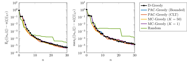
Let us first study the quality of the approximations provided by the different approaches. Figures 1 and 2 represent the evolution of the estimated expectation and maximum, with respect to , of the approximation error for (TC1) and (TC2). These estimates have been computed using independent realizations of obtained from uniform draws of in . In that case, only one realisation of the probabilistic algorithms is performed for the comparison. For both test cases, D-greedy, MC-greedy and PAC-greedy procedures behave similarly with the same error decay with respect to reaching a precision around for (TC1) and for (TC2). Let us mention that for (TC2), the function to approximate has a slow decay of its Kolmogorov -width (see e.g. discussion in [8, Section 4.3.2]) which explains higher error for larger . For the random approach, the selection of interpolation points is less optimal. For first iterates it behaves similarly as other approaches, but we observe that the approximation is less accurate with , from around for (TC1) and for (TC2) respectively. However, despite no guarantee on the optimality of the returned parameter , the PAC algorithm with asymptotic concentration inequality and especially the MC greedy algorithm, either with a single random evaluation of the error estimate (), lead to very satisfactory results with an error close to the deterministic interpolation approach for both test cases.

Greedy procedure.
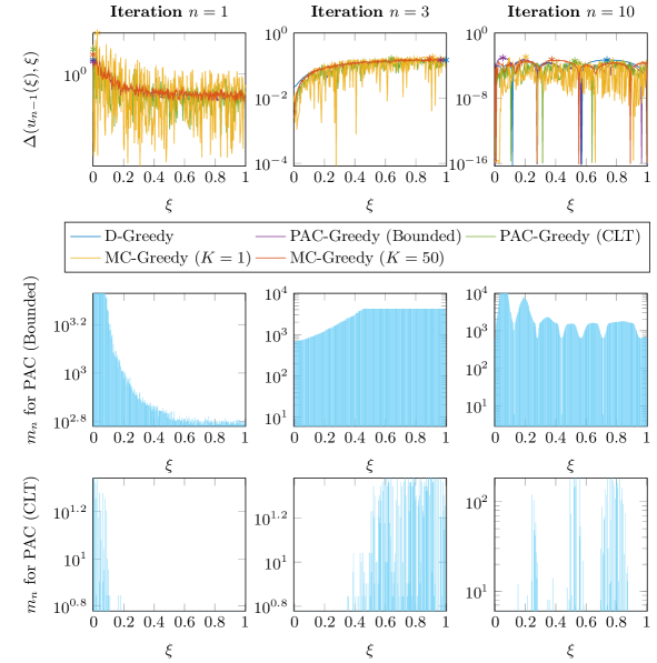
We now turn to the study of the greedy procedures used for the selection of the snapshots. Figures 3-4 represent the error estimate as well as the number of samples required during the greedy selection of for deterministic and probabilistic greedy algorithms based on bandit algorithms for (TC1) and (TC2). These curves corresponds to one realisation of the probabilistic algorithms. First we observe that parameters selected (indicated with the symbol on the curves) by probabilistic algorithms do not necessarily coincide with the ones selected by D-Greedy. For MC-greedy, we observe a much higher variability of the error relatively to parameter , for . This is due to high variance of the estimate. However, in this simple example, even a crude MC estimate with allows to select a value of parameter that will make the error decrease significantly at the next iteration (see Figures 1 and 2). Second, as expected the number of samples is adapted for both algorithms resulting in higher sampling in the region where it is likely to find maximum. Globally, we observe that PAC-greedy (CLT) works quite similarly as PAC-greedy (Bounded). But the two approaches differ in terms of required number of samples. Indeed, CLT based approach only requires around a maximum of samples whereas the one based on concentration inequalities requires between samples.

Sampling complexity.
Now, we briefly discuss the sampling complexities of the different methods, which are summarized in Table 1. From Figures 1 and 2, we see that MC- and PAC-greedy yield roughly the same level of error for a given dimension . Therefore, the table provides the cumulated number of evaluations of the function for constructing the reduced basis of a given dimension for each test case.
| Method | (TC1) for | (TC2) for |
|---|---|---|
| D-Greedy | ||
| MC-Greedy | ||
| MC-Greedy | ||
| PAC-Greedy (Bounded) | ||
| PAC-Greedy (CLT) |
We present as a reference the results of D-greedy using a fine grid for numerical integration. The most costly probabilistic algorithm is PAC-Greedy (Bounded). It requires a high number of samples for constructing non asymptotic confidence intervals, so that it does not outperform D-greedy. Let us mention that PAC-Greedy (CLT) is quite competitive with MC-Greedy with and underlines the interest of using some adaptive procedure for snapshot selection. However, the most interesting trade-off between efficiency and accuracy is MC-Greedy with .
In regard to these observations, in the next section the MC-greedy approach with few samples for the error estimation will be retained in practice to reduce computational costs.
5.2 Parameter-dependent PDE
Now, we focus on the solution of parameter-dependent PDEs, as introduced in Section 4. Given , we seek , solution on of the following boundary problem
| (23) |
for given boundary values and source term . Moreover, we denote and the diffusion and advection coefficients respectively. We assume that (23) admits a unique solution in whose probabilistic representation is given by
The associated parameter-dependent stopped diffusion process is solution of
| (24) |
In the following we take and . The source term as well as Dirichlet boundary conditions are set such that the exact solution to Equation (23) is
| (25) |
5.2.1 Compared procedures
In what follows, we test the probabilistic RBM discussed in Section 4. Since the exact solution is known, we use it for the snapshots. The projection is obtained from evaluations of the exact solution through interpolation (Interp) using magic points or a least-squares (LS) approximation using a set of points in , with . It is also compared to the minimal residual based (MinRes) approximation defined by
| (26) |
During the offline stage, we consider different greedy algorithms for the generation of the reduced spaces. First, we perform the proposed probabilistic greedy Algorithm 3.3 for the construction of the reduced space using MC estimates with defined as in Theorem 4.6.
This approach is compared to an alternative RBM in deterministic setting. Since is implicitly known through the boundary value problem (23), the greedy selection of is performed using Algorithm 2.2 where is an estimate (using trapezoidal integration rule) of the residual based error estimate
during the offline stage.
In the presented results, the residual based greedy algorithm is referred to as Residual. The MC estimate using Feynman-Kac representation is named FK-MC. These approaches are also compared to a naive one named Random in which the parameters that define are chosen at random.
5.2.2 Numerical results
For the numerical experiments, the training set is made of 200 samples from a log uniform distribution over . This distribution is chosen as the solution strongly varies with respect to the viscosity , in particular we want to reach small viscosities. Realizations of , given by (36), are computed using realizations of the approximate stochastic diffusion process solution of Equation (24), obtained by Euler-Maruyama scheme (see Appendix B) with . For computing , magic points are used for interpolation while for LS and MinRes approaches, we choose for a regular grid of points in . Here, greedy algorithms are stopped when . The MC-FK greedy algorithm is performed for .
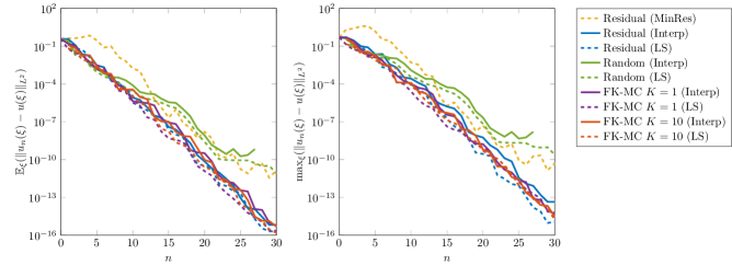
Figure 5 represents the estimated expectation and maximum, with , of the approximation error for the compared procedures, with respect to . The obtained results underline the importance of both projection and reduced basis construction. When MinRes method is used, the approximation is less accurate than for other deterministic approaches (dashed yellow curve). Especially, when it is compared to approaches using a residual based error estimate (blue curves) with interpolation or LS approximation. In that case, the mean approximation error is of order for MinRes against for the latter (for the maximum error, we have against ). Second, let us comment the impact of the probabilistic reduced basis selection. As for function approximation, picking at random the reduced basis for the considered problem is far from optimal since the error expectation tends to stagnate around for (around for the maximum). However, when considering residual based or FK-based error estimates (even with ), with interpolation or least-square for projection, the error behaves quite similarly and reaches for . This shows that the proposed probabilistic based error procedure performs well in practice.
6 Conclusion
In this work we have proposed a probabilistic greedy algorithm for the approximation of a family of parameter-dependent functions for which we only have access to (noisy) pointwise evaluations. It relies on an error indicator that can be written as an expectation of some parameter-dependent random variable.
Different variants of this algorithm have been proposed using either naive MC estimates or PAC bandit algorithms, the latter leading to a weak greedy algorithm with high probability. Several test cases have demonstrated the performances of the proposed procedures.
For parameter-dependent PDEs whose solution admits a probabilistic representation, through the Feynman-Kac formula, such an algorithm can be embedded within a probabilistic RBM using only (noisy) pointwise evaluations. Numerical results have shown the main relevance of considering Feynman-Kac error based estimate for greedy basis selection. We have also illustrated the influence of the projection during online and offline step. Indeed, we observed in Section 5.2.2 that interpolation or least-square projection (using pointwise evaluations of the solution) clearly outperform MinRes projection. Following the discussion of Section 4.2.2, using a sequential procedure as proposed in [5, 18, 19] should be an interesting alternative to avoid limitations of residual based projections. However, further work should be conducted to provide a projection with controlled error and at low cost, which is crucial for efficient model reduction.
The purpose of our simple numerical experiments was to illustrate the behaviour of our probabilistic greedy algorithms. The application to more complex problems in higher dimension will be the focus of future works.
Appendix A Adaptive bandit algorithms
We present an adaptive bandit algorithm to find a PAC maximum in relative precision of over the discrete set . Here is a finite collection of random variables satisfying , defined on the probability space . After introducing some required notation, we present a practical adaptive bandit algorithm which returns a PAC maximum in relative precision for (6) when assuming suitable assumptions on the distribution of .
A.1 Notations and assumptions
We denote by the empirical mean of and its empirical variance, respectively defined by
| (27) |
where are independent copies of . Moreover, the random variable is assumed to satisfy the following concentration inequality
| (28) |
for each , and . The bound depends on the probability distribution of .
Remark A.1.
An alternative to (28) is to rely on asymptotic confidence intervals for based on limit theorems of the form
| (29) |
For example, for second order random variables, the central limit theorem provides such a property with
and the -quantile of the normal distribution.
A.2 Algorithm
Now, let us define a sequence , independent from , and such that .
Then we introduce , and .
Note that the concentration inequality (28) implies that is a confidence interval for with level .
Letting and , we define the following estimate for given by
| (30) |
Then, the adaptive bandit algorithm proposed in [6] is as follows.
Algorithm A.2 (Adaptive bandit algorithm).
| (31) |
At each step , the principle of Algorithm A.2 is to successively increase the number of samples of the random variables in the subset , obtained using confidence intervals of according to (31). The idea behind is to use those confidence intervals to find regions of where one has a high chance to find a maximum. Then, is returned as a maximizer over of the expectation estimate defined by (30). Under suitable assumptions, and when using certified non-asymptotic concentration inequalities, this algorithm returns a PAC maximum in relative precision of over , as stated in [6, Proposition 3.2], recalled below.
Proposition A.3.
Remark A.4.
In general, confidence intervals based on asymptotic theorems are much smaller than those obtained with non-asymptotic concentration inequalities, and yield a selection of much smaller sets of candidate maximizers, hence a much faster convergence of the algorithm. However, when using asymptotic theorems, we can not guarantee to obtain a PAC maximizer.
Appendix B Probabilistic approximation of the solution of a PDE
Here we discuss the numerical computation of an estimate of for any . To that goal, we use a suitable integration scheme to get an approximation of the diffusion process and a MC method to evaluate the expectation in formula (18).
An approximation of the diffusion process is obtained using a Euler-Maruyama scheme. More precisely, setting , , is approximated by a piecewise constant process , where for and
| (34) |
where is an increment of the standard Brownian motion.
Numerical computation of for all requires the computation of a stopped process at time , an estimation of the first exit time of . Here, we consider the simplest way to define this discrete exit time
| (35) |
Such a discretization choice may lead to over-estimation of the exit time with an error in . More sophisticated approaches are possible to improve the order of convergence, as Brownian bridge, boundary shifting or Walk On Sphere (WOS) methods, see e.g., [17, Chapter 6]. These are not considered here.
Letting be independent samples of , we obtain a MC estimate noted for defined as
| (36) |
References
- [1] O. Balabanov and A. Nouy. Randomized linear algebra for model reduction. Part I: Galerkin methods and error estimation. Adv. Comput. Math., 45(5-6):2969–3019, Dec 2019.
- [2] O. Balabanov and A. Nouy. Preconditioners for model order reduction by interpolation and random sketching of operators, 2021.
- [3] O. Balabanov and A. Nouy. Randomized linear algebra for model reduction. Part II: minimal residual methods and dictionary-based approximation. Adv. Comput. Math., 47(2):26–54, Mar 2021.
- [4] M. Bebendorf. Approximation of boundary element matrices. Numerische Mathematik, 86(4):565–589, 2000.
- [5] M. Billaud-Friess, A. Macherey, A. Nouy, and C. Prieur. Stochastic methods for solving high-dimensional partial differential equations. In International Conference on Monte Carlo and Quasi-Monte Carlo Methods in Scientific Computing, pages 125–141. Springer, 2018.
- [6] M. Billaud-Friess, A. Macherey, A. Nouy, and C. Prieur. A PAC algorithm in relative precision for bandit problem with costly sampling. Mathematical Methods of Operations Research, 96(2):161–185, 2022.
- [7] P. Binev, A. Cohen, W. Dahmen, R. DeVore, G. Petrova, and P. Wojtaszczyk. Convergence Rates for Greedy Algorithms in Reduced Basis Methods. SIAM J. Math. Anal., Jun 2011.
- [8] M.-R. Blel, V. Ehrlacher, and T. Lelièvre. Influence of sampling on the convergence rates of greedy algorithms for parameter-dependent random variables. arXiv:2105.14091, May 2021.
- [9] S. Boyaval and T. Lelièvre. A variance reduction method for parametrized stochastic differential equations using the reduced basis paradigm. Commun. Math. Sci., 8(3):735–762, Sep 2010.
- [10] A. Buffa, Y. Maday, A. T. Patera, C. Prud’homme, and G. Turinici. A priori convergence of the greedy algorithm for the parametrized reduced basis method. ESAIM: Mathematical Modelling and Numerical Analysis - Modélisation Mathématique et Analyse Numérique, 46(3):595–603, 2012.
- [11] D. Cai, C. Yao, and Q. Liao. A Stochastic Discrete Empirical Interpolation Approach for Parameterized Systems. Symmetry, 14(3):556, Mar. 2022.
- [12] A. Cohen, W. Dahmen, R. DeVore, and J. Nichols. Reduced basis greedy selection using random training sets. ESAIM: Mathematical Modelling and Numerical Analysis, 54(5):1509–1524, 2020.
- [13] A. Cohen, W. Dahmen, and G. Welper. Adaptivity and variational stabilization for convection-diffusion equations. ESAIM: M2AN, 46(5):1247–1273, Sep 2012.
- [14] A. Cohen and G. Migliorati. Optimal weighted least-squares methods. SMAI Journal of Computational Mathematics, 3:181–203, 2017.
- [15] R. DeVore, G. Petrova, and P. Wojtaszczyk. Greedy Algorithms for Reduced Bases in Banach Spaces. Constr. Approx., 37(3):455–466, Jun 2013.
- [16] A. Friedman. Stochastic Differential Equations and Applications. In Stochastic Differential Equations, pages 75–148. Springer, Berlin, Germany, 2010.
- [17] E. Gobet. Monte-Carlo Methods and Stochastic Processes: From Linear to Non-linear. CRC Press, Boca Raton, FL, USA, 2016.
- [18] E. Gobet and S. Maire. A spectral Monte Carlo method for the Poisson equation. De Gruyter, 10(3-4):275–285, Dec. 2004.
- [19] E. Gobet and S. Maire. Sequential Control Variates for Functionals of Markov Processes on JSTOR. SIAM J. Numer. Anal., 43(3):1256–1275, 2006.
- [20] B. Haasdonk. Reduced Basis Methods for Parametrized PDEs—A Tutorial Introduction for Stationary and Instationary Problems, chapter 2. SIAM, Philadelphia, PA, 2017.
- [21] C. Homescu, L. R. Petzold, and R. Serban. Error Estimation for Reduced-Order Models of Dynamical Systems. SIAM Rev., 49(2):277–299, Jun 2007.
- [22] A. Janon, M. Nodet, C. Prieur, and C. Prieur. Goal-oriented error estimation for parameter-dependent nonlinear problems. ESAIM: Mathematical Modelling and Numerical Analysis, 52(2):705–728, 2018.
- [23] T. Lattimore and C. Szepesvári. Bandit algorithms. Cambridge University Press, Cambridge, England, 2020.
- [24] Y. Maday, N. C. Nguyen, A. T. Patera, and S. H. Pau. A general multipurpose interpolation procedure: the magic points. CPAA, 8(1):383–404, Sept. 2008.
- [25] A. Nouy. Low-Rank Methods for High-Dimensional Approximation and Model Order Reduction, chapter 4. SIAM, Philadelphia, PA, 2017.
- [26] A. Nouy. Low-Rank Tensor Methods for Model Order Reduction. SpringerLink, pages 857–882, Jun 2017.
- [27] A. K. Saibaba. Randomized Discrete Empirical Interpolation Method for Nonlinear Model Reduction. SIAM J. Sci. Comput., May 2020.
- [28] K. Smetana and O. Zahm. Randomized residual-based error estimators for the proper generalized decomposition approximation of parametrized problems. Int. J. Numer. Methods Eng., 121(23):5153–5177, Dec 2020.
- [29] K. Smetana, O. Zahm, and A. T. Patera. Randomized residual-based error estimators for parametrized equations. SIAM journal on scientific computing, 41(2):A900–A926, 2019.
- [30] E. Tyrtyshnikov. Incomplete cross approximation in the mosaic-skeleton method. Computing, 64(4):367–380, 2000.
- [31] O. Zahm and A. Nouy. Interpolation of inverse operators for preconditioning parameter-dependent equations. SIAM Journal on Scientific Computing, 38(2):A1044–A1074, 2016.