Multi-robot Motion Planning based on Nets-within-Nets
Modeling and Simulation

Abstract

This paper focuses on designing motion plans for a heterogeneous team of robots that has to cooperate in fulfilling a global mission. The robots move in an environment containing some regions of interest, and the specification for the whole team can include avoidances, visits, or sequencing when entering these regions of interest. The specification is expressed in terms of a Petri net corresponding to an automaton, while each robot is also modeled by a state machine Petri net. With respect to existing solutions for related problems, the current work brings the following contributions. First, we propose a novel model, denoted High-Level robot team Petri Net (HLPN) system, for incorporating the specification and the robot models into the Nets-within-Nets paradigm. A guard function, named Global Enabling Function (gef), is designed to synchronize the firing of transitions such that the robot motions do not violate the specification. Then, the solution is found by simulating the HPLN system in a specific software tool that accommodates Nets-within-Nets. An illustrative example based on a Linear Temporal Logic (LTL) mission is described throughout the paper, complementing the proposed rationale of the framework.

Discrete event systems, Motion Planning, Multi-robot system

I Introduction

An important part of robotics research is dedicated to planning the motion of mobile agents such that a desired mission is accomplished. Classic scenarios relate to standard navigation problems, where a mobile agent has to reach a desired position without colliding with obstacles [1, 2]. Multiple extensions exist, from which an important part refers to planning a team of mobile robots [3, 4]. At the same time, solutions are proposed for ensuring that the team of robots fulfills a high-level mission, for example visiting some regions only after other regions were explored. Such missions are expressed in various formal languages, such as classes of Temporal Logic formulas [5, 6, 7, 8, 9], Boolean expressions [10], $\mu$-calculus specifications [11, 12].

In general, solutions for the above problems rely on different types of discrete-event-system models for both the mobile robots and the imposed mission. The mobile agents are usually modeled by transition systems or Petri nets (PN), while the specification model has specific forms, such as Büchi automata in the case of Linear Temporal Logic (LTL) tasks. The models for agents and specifications are usually combined, for example, based on a synchronous product of automata, and a solution is found. However, due to the involved synchronous product, the number of states in the resulting discrete-event model may exponentially grow with the number of agents. In the case of identical robots, a PN model for the robotic team has the advantage of maintaining the same topology, irrespective of the team size.

In this work we consider a team of mobile robots evolving in an environment cluttered with regions of interest. The robots may be different, such as some of them can visit only a subset of the regions of interest, and the possible movements of each agent can be modeled by a PN system. The user imposes a global specification over the regions of interest, and we aim in generating motion plans for the agent such that the specification is accomplished. Rather than assuming a specific formal language for the specification, we assume that the task is satisfiable by a finite sequence of movements of the agents, and this task is given in form of a PN. The task can express multiple useful missions for mobile agents, for example, it can include visits of regions of interest based on some conditions (as previously entering some other regions), synchronizations when different agents enter into disjoint regions, or avoidance of some areas until some other are reached. Different than other works, we include both the robots and the task in the same model, and for this, we use the Nets-within-Nets formalism.

The Nets-within-Nets belong to the family of high-level nets, in which each token can transfer information such as the state of another process [13]. For this particular type of net, each token is represented by another net denoted as Object net. The relations between these objects nets and other nets are captured in System net, which contains a global view of the entire system [14].

In the proposed solution, robots are implemented as Object nets. Additionally, the team’s mission is also implemented as an Object net. The interactions between robots and mission models take place via the System net. The model is implemented using the Renew tool [15], which is used to obtain path-planning solutions that accomplish the mission through simulation.

Therefore, the contributions of this paper are as follows:

• Introducing a general framework called the High-Level robot team Petri Net system (HLPN) for path planning a heterogeneous multi-agent robotic system that ensures a global mission;

• Designing a synchronization function (Global Enabling Function) between the nets in the model that verifies and acts on a set of logical Boolean formulas to ensure their correct connotations;

• Incorporating scalability and adaptability properties in the proposed model to address the problem of a flexible number of agents and different spatial constraints with respect to the environment.

In particular, we present a case study based on a partition that maps the environment, an LTL specification as a global mission given to the team of robots, and agents of two different types in terms of their capability of accessing partition regions.

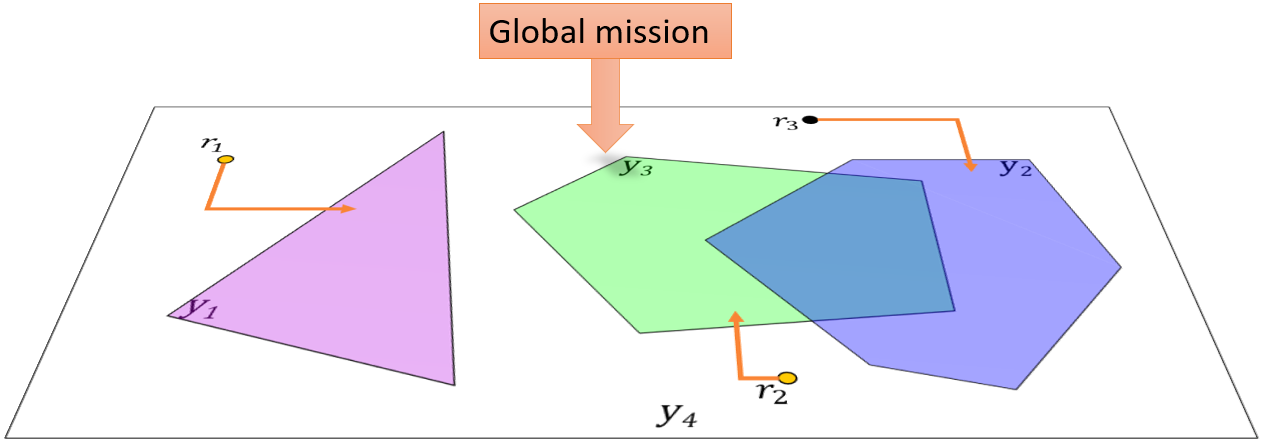
Figure 1: Example of an environment with 3 regions of interest and 3 robots

II Intuitive Reasoning of the proposed approach

Assuming that a global specification for a team of mobile robots is modeled as a PN system, this PN can be referred to as the Specification Object Petri net (SpecOPN) system. It is assumed that a final reachable marking exists, and the formula is satisfied when this marking is reached. Transitions within the SpecOPN are labeled with Boolean formulas and can fire only when they are marking-enabled and their Boolean formulas are evaluated to $True$. This will ensure that the system adheres to the imposed specification.

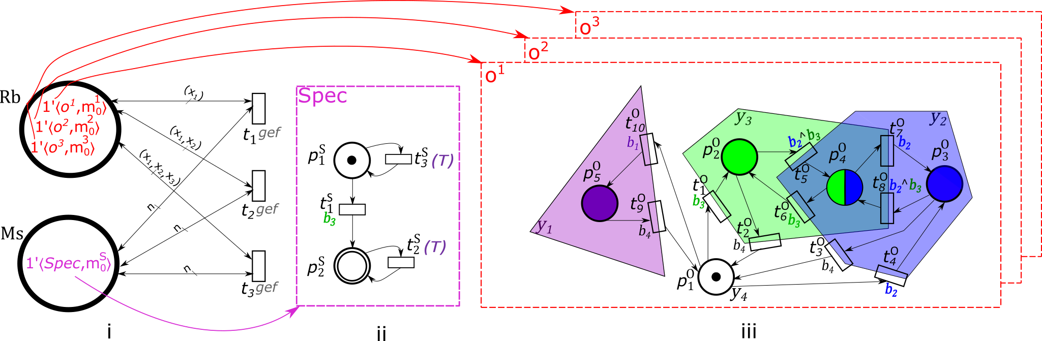
Figure 2: Example of Nets-within-nets formalism: (i) System Petri net, (ii) Specification Object Petri net, (iii) Robotic Object Petri net

An example of a SpecOPN is illustrated in Fig. 2 (ii). In the initial marking, there is one token in $p_{1}^{S}$, and both transitions $t_{1}^{S}$ and $t_{3}^{S}$ are marking-enabled. However, for transition $t_{1}^{S}$ to be fired, the atomic proposition $b_{3}$ must be evaluated as $True$. On the other hand, transition $t_{3}^{S}$ is always fireable at this marking, since it is labeled with $T$ ($True$). The specification is fulfilled when place $p_{2}^{S}$ is marked, which means that transition $t_{1}^{S}$ should fire, and for this proposition $b_{3}$ should become $True$. We note that this SpecOPN models the LTL formula $\diamondsuit b_{3}$ (“eventually $b_{3}$”).

Furthermore, a heterogeneous team of robots is assumed to operate in an environment consisting of several regions denoted $y_{i}$, which may intersect. For each region $y_{i}$ of the environment, an atomic proposition (otherwise known as observation) $b_{i}$ is defined. If a robot is in the region $y_{i}$, the atomic proposition $b_{i}$ evaluates to $True$. As the regions may intersect, more than one atomic proposition may evaluate to $True$. For example, in Fig. 1, if a robot is inside $y_{2}\cap y_{3}$, then both $b_{2}$ and $b_{3}$ are evaluated to $True$, hence the label $b_{2}\wedge b_{3}$ is assigned to the region $y_{2}\cap y_{3}$.

To model each robot, a Robotic Object Petri Net (RobotOPN) is used, where each place represents a part of the environment and it is labeled with a Boolean formula composed of atomic propositions $b_{i}$ corresponding to the environment’s part to which the place belongs. If a place in RobotOPN has one token, the Boolean formula assigned to the place becomes $True$.

As robots evolve within the environment, the truth values of atomic propositions change, thus enabling or disabling transitions in the SpecOPN. For example, Fig. 1, illustrates an example of a 2D environment having four regions of interest $y_{1}$ - purple region, $y_{2}$ - blue region, $y_{3}$ - green region and $y_{4}$ - the free space (white), regions $y_{2}$ and $y_{3}$ being partially overlapped. If all three robots are in region $y_{4}=E\setminus\left(y_{1}\cup y_{2}\cup y_{3}\right)$ ($E$ being the full known environment), only $b_{4}$ is evaluated to $True$, while $b_{1}$, $b_{2}$, and $b_{3}$ are $False$. If robot 1 leaves $y_{4}$ and enters $y_{3}$, by firing transition $t_{1}^{O}$ in the RobotOPN of Fig. 2 (iii), the atomic proposition $b_{3}$ becomes $True$, while $b_{1}$ and $b_{2}$ remain $False$. Since a transition firing in the RobotOPN implies a change in the values of atomic propositions, it must be fired synchronously with a transition in the SpecOPN. In this case, $t_{1}^{O}$ should be fired synchronously with either $t_{1}^{S}$ or $t_{3}^{S}$. Synchronization is accomplished by using a high-level Petri net called the System Petri Net, shown in Fig. 2 (i). Each token in place $Rb$ corresponds to a RobotOPN, while the token in $Ms$ corresponds to the SpecOPN. When a transition $t_{i},i=\overline{1,3}$ is fired, at least one transition from the RobotOPNs and one transition from the SpecOPN are fired synchronously, respecting the conditions imposed by the Global Enabling Function.

III Notations and problem statement

Let us denote a set of regions of interest (ROIs) labeled with $\mathcal{Y}=\{y_{1},y_{2},\dots,y_{|\mathcal{Y}|}\}$, with $|\mathcal{Y}|$ being the cardinality of set $\mathcal{Y}$. We are going to assume that there is a special region that does not intersect with any other region, and that we will call the free space region. For the sake of simplicity, let us assume this region is $y_{|\mathcal{Y}|}$. A mission may specify visits or avoidances of regions $\mathcal{Y}\setminus\{y_{|\mathcal{Y}|}\}$ by a team $\mathcal{R}=\{r_{1},r_{2},\dots r_{|R|}\}$ of omnidirectional mobile robots (agents). Let us also assume that, at the initial state, all the robots are in the free space region. To capture the behavior of the robots in the environment, the continuous space $E$ is partitioned over set $\mathcal{P}_{\mathcal{Y}}=\{p_{1},p_{2},\dots p_{|\mathcal{P}_{\mathcal{Y}}|}\}$ of discrete elements, returned by a mapping technique that preservers the borders of ROIs, e.g., SLAM [16], occupancy grid map [17], cell decomposition [4]. For simplicity, we assume to have the fewest possible number of elements in the partitioned environment $\mathcal{P}_{\mathcal{Y}}$. Thus, in this work, the discrete representation of the workspace is returned by a cell decomposition technique [4] which is further altered into a reduced model denoted Quotient Petri net. This algorithm is described in our work [18].

The result consists in a discrete model of the environment, which can be handled afterwards with respect to the motion of the robots. Each agent has a pre-established set of constraints that defines its allowed movements in $E$. At any moment a robot should physically be placed in one $p\in\mathcal{P}_{\mathcal{Y}}$. In addition, a characteristic of each element $p\in\mathcal{P}_{\mathcal{Y}}$ is represented by its capacity in terms of the maximum number of agents that can be in $p$ at the same time.

Let us denote with $\mathcal{B}_{\mathcal{Y}}=\{b_{1},b_{2},\dots b_{|\mathcal{Y}|}\}$ the set of Atomic Propositions (AP) associated with the set of ROIs $\mathcal{Y}$. The power-set $2^{\mathcal{Y}}$ represents all the combinations of regions of interest. For any subset $A\in 2^{\mathcal{Y}}$ let us define the characteristic conjunction formula of $A$ as $A_{\wedge}=\bigwedge\{b_{i}\in\mathcal{B}_{\mathcal{Y}}\mid y_{i}\in A\}$. For any partition element $p\in\mathcal{P}_{\mathcal{Y}}$, let $h(p)=\{y_{i}\in\mathcal{Y}\mid p\subseteq y_{i}\}$. Let $p_{\wedge}\equiv h(p)_{\wedge}$ be the labeling function that assigns a characteristic conjunction formula to each element $p\in\mathcal{P}_{\mathcal{Y}}$.

This paper considers the following problem:

Problem III.1

Given a heterogeneous multi-agent robotic system in a known environment, and a global mission (specification) requiring visiting and/or avoiding regions of interest, design motion plans for the team of agents such that the specification is fulfilled.

Remark. Although similar problems are studied in the literature [4] (but mainly for identical agents), here we are concerned with designing a different formalism that allows us to combine the motion of the robots with the given specification in the same model. This model is suitable for running simulations in dedicated software tools, and thus the current method obtains a sub-optimal solution through simulations, rather than following the ideas of existing methods that search for an optimal solution by either exploring the reachability graph of various models or solving complex optimization problems.

In this work we solve the motion planning problem for heterogeneous robotic systems with a flexible number of robots, which can synchronize among them. Therefore, we propose a framework that encapsulates the advantages of a compact nested model. The current work models the motion of the robots in a physical workspace with respect to a given mission, all under the Petri net formalism, known as Nets-within-Nets [14]. Such representation allows us to handle various models in a structured manner, which is easier to handle compared with a non-nested structure. In addition, the coordination between different levels of Petri nets benefits from an object-oriented methodology which is applied here in the field of high-level motion planning.

Since the modeling methodology considers high-level Petri nets, the marking of the places will be a multi-set. Given a non-empty set $U$, let $\mu$ be a function $\mu:U\longrightarrow\mathbb{N}$ which assigns a non-negative integer number (coefficient) for each element $u\in U$ [19]. The multi-set $\mu$ over a set $U$ is expressed by: symbol ^′ used for an easier clarity of the multiplicity $u\in U$ and by a symbolic addition $\sum_{u\in U}\mu(u)u$, e.g., $\mu=1^{\prime}u_{1}+2^{\prime}u_{2}$, with $U=\{u_{1},u_{2}\}$. The set of all multi-sets over $U$ is denoted with $Bag(U)$. The algebra of multi-sets is defined in [19], containing multiple operations such as: addition, comparison, which we will omit here due to paper space constraints.

IV Object Petri net systems

As the proposed framework is encapsulated under Nets-within-Nets paradigm, let us define the Object nets that model the given mission for the multi-agent system, and the allowed movements of robots, respectively.

IV-A Specification Object Petri net

The following definition is designated to a subclass of global missions, which can be modeled as a state machine Petri net, being strongly connected, and bounded by one token.

Definition IV.1 (SpecOPN)

A Petri net modeling the global mission given to a multi-agent system is called Specification Object Petri net (SpecOPN) and it is a tuple $Spec=\langle P^{S},P_{f}^{S},T^{S},F^{S},\lambda^{S}\rangle$, where: $P^{S}$ and $T^{S}$ are the disjoint finite set of places and transitions, $P_{f}^{S}\subset P^{S}$ is the set of final places, $F^{S}\subseteq(P^{S}\times T^{S})\cup(T^{S}\times P^{S})$ is the set of arcs. $\lambda^{S}_{\wedge}(t^{S})\equiv t^{S}_{\wedge}$ is the transition labeling function, which assigns to each transition $t^{S}\in T^{S}$ a Boolean formula based on conjunctions of atomic propositions $\mathcal{B}_{\mathcal{Y}}$ or negation of them. A disjunctive Boolean formula assigned to a transition $\lambda^{S}_{\wedge}(t^{S})=b_{i}\vee b_{j}$ is converted into a conjunctive Boolean formula by modifying the topology of $SpecOPN$ such that there exist two transitions with $\lambda^{S}_{\wedge}(t^{S}_{i})=b_{i}$ and $\lambda^{S}_{\wedge}(t^{S}_{j})=b_{j}$. $\Box$

A marking is a $|P^{S}|$-sized natural-valued vector, while a SpecOPN system is a pair $\langle Spec,\mathchoice{\hbox{\boldmath$\displaystyle m$}}{\hbox{\boldmath$\textstyle m$}}{\hbox{\boldmath$\scriptstyle m$}}{\hbox{\boldmath$\scriptscriptstyle m$}}_{0}^{S}\rangle$ where $\mathchoice{\hbox{\boldmath$\displaystyle m$}}{\hbox{\boldmath$\textstyle m$}}{\hbox{\boldmath$\scriptstyle m$}}{\hbox{\boldmath$\scriptscriptstyle m$}}_{0}^{S}$ is the initial marking. The specification is fulfilled when SpecOPN reaches a marking with a token in a place of $P_{f}^{S}$, through firing a sequence of enabled transitions. A transition $t^{S}\in T^{S}$ in the SpecOPN system is enabled at a marking $\mathchoice{\hbox{\boldmath$\displaystyle m$}}{\hbox{\boldmath$\textstyle m$}}{\hbox{\boldmath$\scriptstyle m$}}{\hbox{\boldmath$\scriptscriptstyle m$}}^{S}$ when two conditions are met: (i) $\mathchoice{\hbox{\boldmath$\displaystyle m$}}{\hbox{\boldmath$\textstyle m$}}{\hbox{\boldmath$\scriptstyle m$}}{\hbox{\boldmath$\scriptscriptstyle m$}}^{S}[\,\!^{\bullet}{t^{S}}]=1$ and (ii) the Boolean formula $t^{S}_{\wedge}$ is True. Informally, condition (i) is a witness of the part of the specification already fulfilled, while (ii) means that the movement of the robots with respect to the regions of interest $\mathcal{Y}$ can imply the firing of a transition in SpecOPN by changing the truth value of $t^{S}_{\wedge}$.

For exemplification purposes, we consider SpecOPN associated with a Büchi automaton that can be obtained as in [18], where the global mission to the team is given by a LTL specification. The latter formalism denotes a high-level abstraction of the natural language based on a set of atomic propositions, Boolean and temporal operators, e.g., $\varphi=\diamondsuit b_{3}$ specifies that region $y_{3}$ should be eventually visited, as in Fig. 2. The model of an LTL formula is often represented by a Büchi automaton [20], which accepts only input strings satisfying the LTL formula. In our case, the formula should be satisfiable by a finite string (also known as co-safe LTL), since the SpecOPN has to reach a final marking.

IV-B Robotic Object Petri net

The robotic system which evolves in the known environment can be modeled by a set of Petri nets systems, denoted Robotic Object Petri nets, as each model is assigned to one robot (Fig. 2 (iii)). We assume that the defined model is a state machine PN, where each transition has only one input and one output place. The model can be considered as an extended Labeled Petri net [21] representation by the addition of a labeling function over the set of places.

Definition IV.2 (RobotOPN)

A Robotic Object Petri net modeling the robot $k$ is a tuple $o^{k}=\langle P^{o},T^{o},F^{o},h^{o},\lambda^{o},\gamma^{o}\rangle$:

• $P^{o}$ is the finite set of places, each place being associated to an element $p\in\mathcal{P}_{\mathcal{Y}}$ in which robot $k$ is allowed to enter;

• $T^{o}$ is the finite set of transitions. A transition $t_{ij}^{o}\in T^{o}$ is added between two places $p_{i}^{o},p_{j}^{o}\in P^{o}$ only if the robot $k$ can move from any position in $p_{i}$ to a position in $p_{j}$;

• $F^{o}\subseteq(P^{o}\times T^{o})\cup(T^{o}\times P^{o})$ is the set of arcs. If $t_{ij}^{o}$ is the transition modeling the movement from $p_{i}^{o}$ to $p_{j}^{o}$, then $(p_{i}^{o},t_{ij}^{o})\in F^{o}$ and $(t_{ij}^{o},p_{j}^{o})\in F^{o}$;

• $h^{o}_{\wedge}$ is the labeling function of places $p^{o}\in P^{o}$, defined in the previous section and associating to each place a Boolean formula over the set of propositions $\mathcal{B}_{\mathcal{Y}}$;

• $\lambda^{o}_{\wedge}$ is the Boolean labeling function of transitions $t^{o}\in T^{o}$, such that $\lambda^{o}_{\wedge}(t^{o}_{i})=h\left({t^{{}^{o}}_{i}}^{\bullet}\right)_{\wedge}$;

• $\gamma^{o}:P^{o}\to\mathcal{P}_{\mathcal{Y}}$ is the associating function. If place $p^{o}_{i}\in P^{o}$ is associated to $p_{i}\in\mathcal{P}_{\mathcal{Y}}$, then $\gamma^{o}(p^{o}_{i})=p_{i}$.

Notice that if the robots are omnidirectional, the resulting RobotOPN model is a state machine, which is, indeed, safe. A marking of a RobotOPN is a vector $\mathchoice{\hbox{\boldmath$\displaystyle m$}}{\hbox{\boldmath$\textstyle m$}}{\hbox{\boldmath$\scriptstyle m$}}{\hbox{\boldmath$\scriptscriptstyle m$}}^{k}\in\{0,1\}^{|P^{o}|}$. The initial marking is denoted $\mathchoice{\hbox{\boldmath$\displaystyle m$}}{\hbox{\boldmath$\textstyle m$}}{\hbox{\boldmath$\scriptstyle m$}}{\hbox{\boldmath$\scriptscriptstyle m$}}_{0}^{k}$ such that $\mathchoice{\hbox{\boldmath$\displaystyle m$}}{\hbox{\boldmath$\textstyle m$}}{\hbox{\boldmath$\scriptstyle m$}}{\hbox{\boldmath$\scriptscriptstyle m$}}_{0}^{k}[p^{o}_{i}]=1$ if one robot is initially in $p^{o}_{i}$, and $\mathchoice{\hbox{\boldmath$\displaystyle m$}}{\hbox{\boldmath$\textstyle m$}}{\hbox{\boldmath$\scriptstyle m$}}{\hbox{\boldmath$\scriptscriptstyle m$}}_{0}^{k}[p^{o}_{j}]=0$ for the rest of places $p^{o}_{j}\in P^{o}\setminus\{p^{o}_{i}\}$. A RobotOPN system of robot $r_{k}$ is a pair $\langle o^{k},\mathchoice{\hbox{\boldmath$\displaystyle m$}}{\hbox{\boldmath$\textstyle m$}}{\hbox{\boldmath$\scriptstyle m$}}{\hbox{\boldmath$\scriptscriptstyle m$}}^{k}_{0}\rangle$.

The heterogeneity of the robotic system relates to the differences in RobotOPN models in terms of topology and labels.

V System Petri Net and Global Enabling Function

V-A System Petri net

This subsection introduces the System Petri Net for the motion planning problem, being denoted with High-Level robot team Petri net. This representation is designed to enable synchronization among the robots and specification net models, following the Nets-within-Nets paradigm.

Definition V.1

A High-Level robot team Petri net (HLPN) is a tuple ${\mathcal{N}}=\langle P,T,\mathcal{O},\mathcal{S},Vars,F,W,\mu_{cap}\rangle$, where:

• $P=\left\{Rb,Ms\right\}$ is the set of places;

• $T=\{t_{1},t_{2},\ldots,t_{|R|}\}$ is the set of transitions;

• $\mathcal{O}=\{\langle o^{1},\mathchoice{\hbox{\boldmath$\displaystyle m$}}{\hbox{\boldmath$\textstyle m$}}{\hbox{\boldmath$\scriptstyle m$}}{\hbox{\boldmath$\scriptscriptstyle m$}}_{0}^{1}\rangle,\langle o^{2},\mathchoice{\hbox{\boldmath$\displaystyle m$}}{\hbox{\boldmath$\textstyle m$}}{\hbox{\boldmath$\scriptstyle m$}}{\hbox{\boldmath$\scriptscriptstyle m$}}_{0}^{2}\rangle,\ldots,\langle o^{|R|},\mathchoice{\hbox{\boldmath$\displaystyle m$}}{\hbox{\boldmath$\textstyle m$}}{\hbox{\boldmath$\scriptstyle m$}}{\hbox{\boldmath$\scriptscriptstyle m$}}_{0}^{|R|}\rangle\}$ is a set of $|R|$ RobotOPN systems, one for each robot;

• $\mathcal{S}=\langle Spec,\mathchoice{\hbox{\boldmath$\displaystyle m$}}{\hbox{\boldmath$\textstyle m$}}{\hbox{\boldmath$\scriptstyle m$}}{\hbox{\boldmath$\scriptscriptstyle m$}}_{0}^{S}\rangle$ is a SpecOPN system;

• $Vars=\{n,x_{1},x_{2},\ldots,x_{|R|}\}$ is a set of variables;

• $F$ is the set of arcs: $\forall t\in T$ and $\forall p\in P$, $(t,p)\in F$ and $(p,t)\in F$;

• $W$ is the inscription function assigning to each arc a set of variables from $Vars$ such that for every $t_{i}\in T$, $W(Rb,t_{i})=W(t_{i},Rb)=(x_{1},x_{2},\ldots,x_{i})$, $W(Ms,t_{i})=W(t_{i},Ms)=n$;

• $\mu_{cap}\in Bag(\mathcal{P}_{\mathcal{Y}})$ is the capacity multi-set, with $\mu_{cap}[p_{i}]>0,\forall i\in\{1,\ldots,|\mathcal{P}_{\mathcal{Y}}|-1\}$ and $\mu_{cap}[p_{|\mathcal{P}_{\mathcal{Y}}|}]\leq|R|$.

$Rb$ and $Ms$ are called, respectively, the robot and mission places. Transition $t_{i}$ is used for the synchronized movement of $i$ robots according to the specification (this is the reason for having exactly $|R|$ transitions). Furthermore, each element $p_{i}\in\mathcal{P}_{\mathcal{Y}}$ has a given number of space units, its capacity. The capacity of each discrete element $p_{i}$ (the maximum number of robots that can exist simultaneously in $p_{i}$) is $\mu_{cap}[p_{i}]$, being given by the multi-set $\mu_{cap}$. Therefore, each element $p_{i}\in\mathcal{P}_{\mathcal{Y}}$ has a strictly positive capacity, considering that the free space $p_{|\mathcal{P}_{\mathcal{Y}}|}$ can accommodate the whole team, as mentioned in the last bullet of Def. V.1

Notice in Fig. 2 (i) that the places $Rb$ and $Ms$ are connected with the transitions via bidirectional arcs. The firing of a transition manipulates an Object net through the use of variables, e.g., $x_{1}$ is bound to RobotOPN $o^{1}$. Although the state of an Object net is modified when a transition in the HLPN system is fired, by using the reference semantics as in [14], a token is a reference to an Object net, the same variable being used for both directions: from place towards transitions, respectively vice-versa.

A HLPN system is a tuple $\langle{\mathcal{N}},\mathchoice{\hbox{\boldmath$\displaystyle m$}}{\hbox{\boldmath$\textstyle m$}}{\hbox{\boldmath$\scriptstyle m$}}{\hbox{\boldmath$\scriptscriptstyle m$}},\mu_{occ}\rangle$ where ${\mathcal{N}}$ is a HLPN as in Def. V.1, $m$ is the marking associating to each place in $P$ a multi-set. The initial marking $\mathchoice{\hbox{\boldmath$\displaystyle m$}}{\hbox{\boldmath$\textstyle m$}}{\hbox{\boldmath$\scriptstyle m$}}{\hbox{\boldmath$\scriptscriptstyle m$}}_{0}$ is

• $\mathchoice{\hbox{\boldmath$\displaystyle m$}}{\hbox{\boldmath$\textstyle m$}}{\hbox{\boldmath$\scriptstyle m$}}{\hbox{\boldmath$\scriptscriptstyle m$}}_{0}[R_{b}]=1^{\prime}\langle o^{1},\mathchoice{\hbox{\boldmath$\displaystyle m$}}{\hbox{\boldmath$\textstyle m$}}{\hbox{\boldmath$\scriptstyle m$}}{\hbox{\boldmath$\scriptscriptstyle m$}}_{0}^{1}\rangle+1^{\prime}\langle o^{2},\mathchoice{\hbox{\boldmath$\displaystyle m$}}{\hbox{\boldmath$\textstyle m$}}{\hbox{\boldmath$\scriptstyle m$}}{\hbox{\boldmath$\scriptscriptstyle m$}}_{0}^{2}\rangle+\ldots+1^{\prime}\langle o^{|R|},\mathchoice{\hbox{\boldmath$\displaystyle m$}}{\hbox{\boldmath$\textstyle m$}}{\hbox{\boldmath$\scriptstyle m$}}{\hbox{\boldmath$\scriptscriptstyle m$}}_{0}^{|R|}\rangle$;

• $\mathchoice{\hbox{\boldmath$\displaystyle m$}}{\hbox{\boldmath$\textstyle m$}}{\hbox{\boldmath$\scriptstyle m$}}{\hbox{\boldmath$\scriptscriptstyle m$}}_{0}[Ms]=1^{\prime}\langle Spec,\mathchoice{\hbox{\boldmath$\displaystyle m$}}{\hbox{\boldmath$\textstyle m$}}{\hbox{\boldmath$\scriptstyle m$}}{\hbox{\boldmath$\scriptscriptstyle m$}}_{0}^{S}\rangle$.

Finally, $\mu_{occ}\in Bag(\mathcal{B}_{\mathcal{Y}})$ is the occupancy multi-set representing the actual position of the robots with respect to $\mathcal{Y}$. At a given time, $\mu_{occ}[b_{i}]$ is the actual number of robots in the region $y_{i}$. The initial occupancy multi-set is $\mu_{occ_{0}}=\sum_{i=1}^{\mathcal{|B_{\mathcal{Y}}|}-1}0^{\prime}b_{i}+|R|{{}^{\prime}b_{|\mathcal{Y}|}}$ since we assume that initially, all robots are in the free space region.

A transition $t\in T$ of the HLPN is enabled at a given state $\langle\mathchoice{\hbox{\boldmath$\displaystyle m$}}{\hbox{\boldmath$\textstyle m$}}{\hbox{\boldmath$\scriptstyle m$}}{\hbox{\boldmath$\scriptscriptstyle m$}},\mu_{occ}\rangle$ iff

• $\mathchoice{\hbox{\boldmath$\displaystyle m$}}{\hbox{\boldmath$\textstyle m$}}{\hbox{\boldmath$\scriptstyle m$}}{\hbox{\boldmath$\scriptscriptstyle m$}}[Ms]$ has a transition $t^{S}\in T^{S}$ enabled;

• being $W(Rb,t)=(x_{1},x_{2},\ldots,x_{i})$, $\mathchoice{\hbox{\boldmath$\displaystyle m$}}{\hbox{\boldmath$\textstyle m$}}{\hbox{\boldmath$\scriptstyle m$}}{\hbox{\boldmath$\scriptscriptstyle m$}}[Rb]$ has $i$ RobotOPN net systems $(\langle o^{1},\mathchoice{\hbox{\boldmath$\displaystyle m$}}{\hbox{\boldmath$\textstyle m$}}{\hbox{\boldmath$\scriptstyle m$}}{\hbox{\boldmath$\scriptscriptstyle m$}}^{1}\rangle,\langle o^{2},\mathchoice{\hbox{\boldmath$\displaystyle m$}}{\hbox{\boldmath$\textstyle m$}}{\hbox{\boldmath$\scriptstyle m$}}{\hbox{\boldmath$\scriptscriptstyle m$}}^{2}\rangle,\ldots,\langle o^{i},\mathchoice{\hbox{\boldmath$\displaystyle m$}}{\hbox{\boldmath$\textstyle m$}}{\hbox{\boldmath$\scriptstyle m$}}{\hbox{\boldmath$\scriptscriptstyle m$}}^{i}\rangle)$ such that each of these nets has a transition $t^{o^{j}}$ enabled, with $j=\overline{1,i}$, and also $gef(\mu_{occ},\mu_{cap},t^{S},(t^{o^{1}},t^{o^{2}},\ldots t^{o^{i}}))=1$ .

An enabled transition $t\in T$ may fire yielding the system from $\langle\mathchoice{\hbox{\boldmath$\displaystyle m$}}{\hbox{\boldmath$\textstyle m$}}{\hbox{\boldmath$\scriptstyle m$}}{\hbox{\boldmath$\scriptscriptstyle m$}},\mu_{occ}\rangle$ to $\langle\mathchoice{\hbox{\boldmath$\displaystyle m$}}{\hbox{\boldmath$\textstyle m$}}{\hbox{\boldmath$\scriptstyle m$}}{\hbox{\boldmath$\scriptscriptstyle m$}}^{\prime},\mu_{occ}^{\prime}\rangle$ such that,

• $\mathchoice{\hbox{\boldmath$\displaystyle m$}}{\hbox{\boldmath$\textstyle m$}}{\hbox{\boldmath$\scriptstyle m$}}{\hbox{\boldmath$\scriptscriptstyle m$}}^{\prime}[Ms]$ has fired transition $t^{S}$;

• at $\mathchoice{\hbox{\boldmath$\displaystyle m$}}{\hbox{\boldmath$\textstyle m$}}{\hbox{\boldmath$\scriptstyle m$}}{\hbox{\boldmath$\scriptscriptstyle m$}}^{\prime}[Rb]$, each $o^{i}$ has fired transition $t^{o^{i}}$;

• $\mu_{occ}^{\prime}$ is updated based on the new position of the robots.

V-B The Global Enabling Function (gef)

When firing a HLPN transition $t_{j}\in T$, the system must coordinate transitions in both RobotOPNs from $\mathchoice{\hbox{\boldmath$\displaystyle m$}}{\hbox{\boldmath$\textstyle m$}}{\hbox{\boldmath$\scriptstyle m$}}{\hbox{\boldmath$\scriptscriptstyle m$}}[Rb]$ and SpecOPN from $\mathchoice{\hbox{\boldmath$\displaystyle m$}}{\hbox{\boldmath$\textstyle m$}}{\hbox{\boldmath$\scriptstyle m$}}{\hbox{\boldmath$\scriptscriptstyle m$}}[Mb]$. However, this synchronization must comply with multiple compatibility rules that take into account the current state of the system, including $\mu_{occ}$. To ensure that these rules are satisfied, the Global Enabling Function (gef) acts as a gatekeeper (guard), verifying the compatibility of the system’s state with the transition rules before enabling the synchronous transitions. The gef plays a critical role in ensuring that the firing of a HLPN transition, along with its associated RobotOPNs and SpecOPN enabled transitions, can proceed without violating any rules.

For any transition $t\in T$, gef takes inputs from $Bag(\mathcal{P}_{\mathcal{Y}})\times Bag(\mathcal{B}_{y})\times T^{S}\times\left(\bigcup_{i=1}^{|R|}\prod_{j=1}^{i}T_{j}^{O}\right)$, and returns either $True$ or $False$ to enable or disable $t$. The gef considers the assignment of variables to the input arcs (i.e., $n$ and $(x_{1},x_{2},\ldots x_{i})$), along with global information such as the occupancy multi-set $\mu_{occ}$, the capacity multi-set $\mu_{cap}$, a marking-enabled transition $t^{S}$ in the SpecOPN $n$, and a set of $i$ marking-enabled transitions $(t^{o^{1}},t^{o^{2}},\ldots t^{o^{i}})$ in $(x_{1},x_{2},\ldots x_{i})$. If by the firing of the $i$ transitions in the RobotOPN the Boolean label assigned to $t^{S}$ is satisfied then gef returns $True$; otherwise, it returns $False$. The algorithm of this function is shown in Alg. 1.

Input: $\mu_{occ},\mu_{cap},t^{S},(t^{o^{1}},t^{o^{2}},\ldots t^{o^{i}})$

Output: $True$ or $False$

Data: $(\langle o^{1},\mathchoice{\hbox{\boldmath$\displaystyle m$}}{\hbox{\boldmath$\textstyle m$}}{\hbox{\boldmath$\scriptstyle m$}}{\hbox{\boldmath$\scriptscriptstyle m$}}^{1}\rangle,\langle o^{2},\mathchoice{\hbox{\boldmath$\displaystyle m$}}{\hbox{\boldmath$\textstyle m$}}{\hbox{\boldmath$\scriptstyle m$}}{\hbox{\boldmath$\scriptscriptstyle m$}}^{2}\rangle,\ldots,\langle o^{|R|},\mathchoice{\hbox{\boldmath$\displaystyle m$}}{\hbox{\boldmath$\textstyle m$}}{\hbox{\boldmath$\scriptstyle m$}}{\hbox{\boldmath$\scriptscriptstyle m$}}^{|R|}\rangle),\mathcal{P}_{\mathcal{Y}}$

1 Let $\chi$ be the simulated occupancy multi-set w.r.t. $\mathcal{P}_{\mathcal{Y}}$ after firing $(t^{o^{1}},t^{o^{2}},\ldots t^{o^{i}})$;

2 forall $p_{j}\in\mathcal{P}_{\mathcal{Y}}$ do

3       if $\left(\chi[p_{j}]>\mu_{cap}[p_{j}]\right)$/* if the capacity of $p_{j}$ will not be satisfied */

4       then

5             return $False$

6      

7 if  $\left(t^{S}_{\wedge}==True\right)$/* if the label of the enabled transition in the SpecOPN is $True$ */

8 then

9      return $True$

10 else

11       Let $\mu_{occ}^{\prime}$ be the simulated update of $\mu_{occ}$ w.r.t. $\mathcal{B}_{\mathcal{Y}}$ after firing $(t^{o^{1}},t^{o^{2}},\ldots t^{o^{i}})$;

12       forall $\left(b_{j}\in\mathcal{B}_{\mathcal{Y}}\right)$ do

13             if $\left(b_{j}\in t^{S}_{\wedge}\land\mu_{occ}^{\prime}[b_{j}]==0\right)\lor\left(\neg b_{j}\in t^{S}_{\wedge}\land\mu_{occ}^{\prime}[b_{j}]\geq 1\right)$  then

14                   return $False$

15            

16       return $True$

17

Algorithm 1 The Global Enabling Function (gef)

The verification of enabling a transition $t\in T$ is made possible via the simulation of the firing of the corresponding $i$ transitions in RobotOPN synchronized by means of transition $t_{i}$ of the HLPN. This artificial process is carried out by the simulation of multi-set $\chi$ which is computed (line 1). In order to compute it, transitions $(t^{o^{1}},t^{o^{2}},\ldots,t^{o^{i}})$ are fictitiously fired in the corresponding RobotOPN (from $o^{1}$ to $o^{i}$), while in the rest of RobotOPN (from $o^{i+1}$ to $o^{|\mathcal{R}|}$) no transition is fired. Thus, the marked places of all RobotOPN are considered. By using the associating function $\gamma^{o}$ in each RobotOPN, multi-set $\chi$ is obtained. Next, the gef verifies that the firing of transitions satisfies the capacity of each $p_{j}\in\mathcal{P}_{\mathcal{Y}}$ (line 1-1).

If the capacity constraints are satisfied and the Boolean formula assigned to $t^{S}$ (i.e., $t^{S}_{\wedge}$) is identical with $True$, then the transitions $\langle t^{S},(t^{o^{1}},t^{o^{2}},\ldots,t^{o^{i}})\rangle$ can fire synchronously without being necessary the evaluation w.r.t. robots positions. As a result, the gef returns $True$ (line 1).

Otherwise, a new simulation is performed and $\mu_{occ}^{\prime}$ is updated. Notice that $\chi$, respectively $\mu_{occ}^{\prime}$ represent the simulated occupancy multi-sets w.r.t. $\mathcal{P}_{\mathcal{Y}}$, respectively $\mathcal{B}_{\mathcal{Y}}$. In the case of $\mu_{occ}^{\prime}$, there are two additional conditions that could prevent the considered transitions to fire. These conditions are checked in lines 1-1 and can be described as:

• If an atomic proposition $b_{j}\in\mathcal{B}_{\mathcal{Y}}$ is part of the formula $t^{S}_{\wedge}$, but in the simulated occupancy state obtained by the firing of the transitions ($\mu_{occ}^{\prime}$), no robot will be in $y_{j}$, then this movement of robots does not fulfill the Boolean function assigned to the transition $t^{S}$ (first condition in line 1).

• If a negated atomic proposition $\neg b_{j}$ (with $b_{j}\in\mathcal{B}_{\mathcal{Y}}$) is part of the $t^{S}_{\wedge}$ formula, but the simulated update of the occupancy $\mu_{occ}^{\prime}$ after the firing of the involved transitions is such that $\mu_{occ}^{\prime}[b_{i}]>1$, this means that one robot would be in $y_{j}$ and the formula $t^{S}_{\wedge}$ would not be fulfilled (second condition in line 1).

If at least one of the previous conditions is true, then the gef will return $False$ (line 1). Otherwise, it will return $True$ (line 1). The firing of a transition $t$ updates the marking of the system and the multi-set $\mu_{occ}$.

VI Simulations

VI-A RENEW Implementation

The proposed framework is implemented in the Renew software tool [22], which is a Java-based high-level Petri net simulator suitable for modeling the Nets-within-Nets paradigm in a versatile approach, based on transitions labels, and Java functions among others.

As mentioned in the beginning of the paper, the proposed framework is assessed through simulations. The simulations return non-deterministic solutions for the paths of the robots, as there are several possibilities to verify the Boolean formulas required by the SpecOPN. Based on the versatility of the algorithmic approach for the current work, several metrics can be defined to assess the quality of simulations. In the following study case, we will refer to the shortest paths of robots out of a given total number of simulations, based on the number of fired transitions in each RobotOPN assigned to the motion of each agent. Of course, this does not guarantee that obtained robotic plans yield the optimal possible value for the chosen metric, but only the best one from the performed set of simulations.

For an easier visualization in the Renew simulator, let us define notations without subscripts. Thus, let $\mathcal{Y}=\{c,b,a,free\}$ be the set of atomic propositions replacing the set $\mathcal{B}_{\mathcal{Y}}$ associated with set $\mathcal{Y}$, such that $c\equiv b_{1},b\equiv b_{2},a\equiv b_{3}$, and $b_{4}\equiv free$. In addition, the symbols $\neg$ or $\wedge$ are replaced in Renew with the syntax “$!$“, respectively “,“. The Specification net models a Büchi automaton assigned to the given LTL formula (described in the next sub-section), thus the $True$ value in the automaton is expressed in Renew through “1“. The elements of the partitioned workspace are associated with the regions of interest in such way: $p_{1}$ for region $y_{1}$, $p_{2}$ for the overlapped area $y_{2}\cap y_{3}$, $p_{3}$ for area $y_{3}\setminus y_{2}$, $p_{4}$ for free space $y_{4}$, while $p_{5}$ for area $y_{2}\setminus y_{3}$. In the following, one example is provided in addition to the mathematical formalism described throughout the paper.

VI-B Case-study

Let us provide a complete example tackling the problem formulation from Sec. III. We exemplify a path planning strategy for a team of three robots evolving in a known workspace (Fig. 1) for which a global specification is given, using the Linear Temporal Logic language. The mission $\varphi=\diamondsuit b_{3}\wedge\diamondsuit b_{2}\wedge\diamondsuit b_{1}\wedge\left(\neg b_{3}~{}\mathcal{U}~{}b_{1}\right)$ implies the visit of regions of interest $y_{1},y_{2},y_{3}$, but requires that region $y_{3}$ to be visited before $y_{1}$.

From the point of view of multi-agent spatial constraints, each partition element has a maximum capacity equal with two, e.g., $\mu_{cap}[p_{1}]=2$ means that no more than two robots can be present at the same time in the area $p_{1}$, where $p_{1}$ is the partition element corresponding to $y_{1}$. The robots are different w.r.t. to their spacial capabilities, in the sense that robots $r_{1}$ and $r_{2}$ are allowed to move freely in the entire environment, while robot $r_{3}$ cannot reach the overlapping part of regions $y_{2}$ and $y_{3}$, denoted with partition element $p_{2}$ in Fig. 3.

For each agent of the team, one RobotOPN is built as follows: $r_{1},r_{2}$ are modeled identically by $o^{1},o^{2}$, while $r_{3}$ is modeled by $o^{3}$ (Fig. 2 (iii)), which are represented in Renew as in Fig. 3. The SpecOPN (Fig. 4) is represented by the Büchi Petri net assigned to the mentioned LTL formula, based on the algorithm from [18].

Out of 100 simulations (the execution time per simulation was 18 milliseconds in mean, with a standard deviation of 12 milliseconds), we could compute the shortest path of the multi-agent system in terms of the truth values of atomic propositions, such as: $\langle r_{1},r_{2},r_{3}\rangle=\langle b_{1},b_{3},b_{2}\rangle$, meaning that $r_{1},r_{2}$ respectively $r_{3}$ moves synchronously into regions $y_{1},y_{3}$, respectively $y_{2}$. The motion of the robots is synchronized (based on the truth value of $gef$) by firing the most right transition in SpecOPN, having the Boolean label $b_{1}\wedge b_{2}\wedge b_{3}$ (blue path in Fig. 4). As mentioned before, Renew returns non-deterministic solutions. Therefore, other path in the SpecOPN (purple color) can be returned by another run of 100 simulations, having as robots shortest paths $\langle r_{1},r_{2},r_{3}\rangle=\langle b_{2},b_{1},b_{2}\rangle,\langle free,b_{1}\wedge b_{3},free\rangle$, meaning that firstly $r_{1},r_{3}$ move to region $y_{2}$, while $r_{2}$ moves towards $y_{3}$; secondly $r_{1},r_{3}$ returns to the free space $y_{4}$, while $r_{2}$ reaches the overlapped area of $y_{2}\cap y_{3}$.

Notice that if the number of robots in the team decreases, having one robot for each type, then the shortest path of the multi-agent system will be longer compared with the formerly result, due to the fact that the transition in SpecOPN model with label $b_{1}\wedge b_{2}\wedge b_{3}$ cannot be fired.

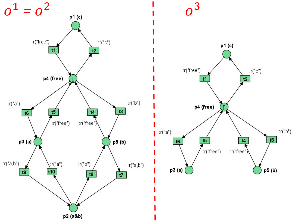
Figure 3: RobotOPN models in Renew tool: $r_{1}$ and $r_{2}$ can move freely in the workspace (left side), while $r_{3}$ is not allowed to enter the overlapped region between $y_{2}$ and $y_{3}$ (right side)

The entire implementation of this example can be accessed on the GitHub link.

Although our approach provides a scalable and independent method of modeling the motion of heterogeneous systems based on RobotOPN’s structure topology, two questions are raised in terms of (i) inferring the computational tractability scales when the number of robots increases, and (ii) encapsulating time constraints under high-level Petri nets formalism, which would be suitable in the motion planning field.

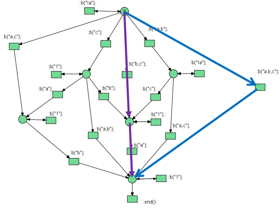
Figure 4: Paths followed by the robotic system in the SpecPN, based on the shortest path of robots out of 100 simulations

VII Conclusion

This paper tackles the problem of motion planning for a team of heterogeneous robots while ensuring a global mission that includes visits and avoidances of some regions of interest. The planning strategy is returned by a newly proposed framework under the Nets-within-Nets paradigm, denoted High-Level robot team Petri net. Specifically, the current work offers an adaptable and flexible solution with respect to the number of agents in the team, by formally defining the model and simulating it for a case study. The approach makes use of the advantages of nested high-level Petri nets systems, such as object-oriented methodology, by modeling the movement of the robots as a set of Robotic Object Petri nets, while the given mission is modeled by a Specification Petri net. These nets become part of a so-called System Petri net, which coordinates their transitions, contributing to a globa view of the entire robotic system due to the fact that the Object nets are represented as tokens in the latter net. Moreover, the relation between the nets is directed by a guard denoted Global Enabling Function. Thus, the synchronization between the nets is handled by the nested structure of the proposed model, joined by the designed guard function.

Future work envisions handling collaborative tasks assignments of the robotic systems, based on multiple missions given to sub-groups of robots. In addition, we are interested in coordinating the Object Petri net when time constraints are added next to space constraints, under the proposed High-Level robot team Petri net system.

References

- [1] H. Choset, K. Lynch, S. Hutchinson, G. Kantor, W. Burgard, L. Kavraki, and S. Thrun, Principles of Robot Motion: Theory, Algorithms, and Implementations. MIT Press, May 2005.
- [2] S. M. LaValle, Planning Algorithms. Cambridge University Press, United Kingdom, 2006.
- [3] C. Belta, A. Bicchi, M. Egerstedt, E. Frazzoli, E. Klavins, and G. Pappas, “Symbolic planning and control of robot motion,” IEEE Robotics and Automation Magazine, vol. 14, no. 1, pp. 61–71, 2007.
- [4] C. Mahulea, M. Kloetzer, and R. González, Path Planning of Cooperative Mobile Robots Using Discrete Event Models. John Wiley & Sons, 2020.
- [5] H. Kress-Gazit, G. E. Fainekos, and G. J. Pappas, “Temporal-logic-based reactive mission and motion planning,” IEEE Transactions on Robotics, vol. 25, no. 6, pp. 1370–1381, 2009.
- [6] M. Guo, J. Tumova, and D. Dimarogonas, “Cooperative decentralized multi-agent control under local ltl tasks and connectivity constraints,” in IEEE Conference on Decision and Control, Los Angeles, CA, USA, 2014, pp. 75 – 80.
- [7] L. Lindemann and D. V. Dimarogonas, “Robust motion planning employing signal temporal logic,” in 2017 American Control Conference (ACC). IEEE, 2017, pp. 2950–2955.
- [8] N. Mehdipour, C.-I. Vasile, and C. Belta, “Specifying user preferences using weighted signal temporal logic,” IEEE Control Systems Letters, vol. 5, no. 6, pp. 2006–2011, 2020.
- [9] X. Yu, X. Yin, S. Li, and Z. Li, “Security-preserving multi-agent coordination for complex temporal logic tasks,” Control Engineering Practice, vol. 123, pp. 105–130, 2022.
- [10] C. Mahulea, M. Kloetzer, and J.-J. Lesage, “Multi-robot path planning with boolean specifications and collision avoidance,” IFAC-PapersOnLine, vol. 53, no. 4, pp. 101–108, 2020.
- [11] S. Karaman and E. Frazzoli, “Sampling-based motion planning with deterministic -calculus specifications,” in 48h IEEE Conference on Decision and Control (CDC). IEEE, 2009, pp. 2222–2229.
- [12] E. Plaku and S. Karaman, “Motion planning with temporal-logic specifications: Progress and challenges,” AI communications, vol. 29, no. 1, pp. 151–162, 2016.
- [13] K. Jensen and G. Rozenberg, High-level Petri nets: theory and application. Springer Science & Business Media, 2012.
- [14] R. Valk, “Object petri nets,” in Advanced Course on Petri Nets. Springer, 2003, pp. 819–848.
- [15] L. Cabac, M. Haustermann, and D. Mosteller, “Renew 2.5–towards a comprehensive integrated development environment for petri net-based applications,” in Application and Theory of Petri Nets and Concurrency: 37th International Conference, PETRI NETS 2016, Toruń, Poland, June 19-24, 2016. Proceedings 37. Springer, 2016, pp. 101–112.
- [16] Y. Chen, S. Huang, and R. Fitch, “Active slam for mobile robots with area coverage and obstacle avoidance,” IEEE/ASME Transactions on Mechatronics, vol. 25, no. 3, pp. 1182–1192, 2020.
- [17] A. Elfes, “Using occupancy grids for mobile robot perception and navigation,” Computer, vol. 22, no. 6, pp. 46–57, 1989.
- [18] S. Hustiu, C. Mahulea, M. Kloetzer, and J.-J. Lesage, “On multi-robot path planning based on Petri net models and LTL specifications,” 2022. [Online]. Available: https://arxiv.org/abs/2211.04230
- [19] K. Jensen, “Coloured Petri nets: A high level language for system design and analysis,” in High-level Petri Nets. Berlin, Heidelberg: Springer Berlin Heidelberg, 1991, pp. 44–119.
- [20] P. Wolper, M. Vardi, and A. Sistla, “Reasoning about infinite computation paths,” in Proceedings of the 24th IEEE Symposium on Foundations of Computer Science, E. N. et al., Ed., Tucson, AZ, 1983, pp. 185–194.
- [21] M. P. Cabasino, A. Giua, M. Pocci, and C. Seatzu, “Discrete event diagnosis using labeled Petri nets. an application to manufacturing systems,” Control Engineering Practice, vol. 19, no. 9, pp. 989–1001, 2011.
- [22] O. Kummer, F. Wienberg, M. Duvigneau, M. Köhler, D. Moldt, and H. Rölke, “Renew–the reference net workshop,” in Tool Demonstrations, 21st International Conference on Application and Theory of Petri Nets, Computer Science Department, Aarhus University, Aarhus, Denmark, 2000, pp. 87–89.