STRAP: Structured Transformer for
Affordance Segmentation with Point Supervision

Abstract

With significant annotation savings, point supervision has been proven effective for numerous 2D and 3D scene understanding problems. This success is primarily attributed to the structured output space; i.e., samples with high spatial affinity tend to share the same labels. Sharing this spirit, we study affordance segmentation with point supervision, wherein the setting inherits an unexplored dual affinity—spatial affinity and label affinity. By label affinity, we refer to affordance segmentation as a multi-label prediction problem: A plate can be both holdable and containable. By spatial affinity, we refer to a universal prior that nearby pixels with similar visual features should share the same point annotation. To tackle label affinity, we devise a dense prediction network that enhances label relations by effectively densifying labels in a new domain (i.e., label co-occurrence). To address spatial affinity, we exploit a Transformer backbone for global patch interaction and a regularization loss. In experiments, we benchmark our method on the challenging CAD120 dataset, showing significant performance gains over prior methods. We provide access to the codebase of our work at https://github.com/LeiyaoCui/STRAP.

1 Introduction

Computer vision has extensively explored the synergy between low- and high-level affinity. For example, superpixels—the perceptual grouping of pixels—can facilitate object segmentation with much fewer computational efforts: Two nearby pixels likely belong to the same object (high-level affinity) if they carry similar colors (low-level affinity). Sharing a similar spirit, Graph Cuts [2], a representative method in segmentation, propagates the source’s label and a sink point to the entire image for globally optimal segmentation. In the era of deep learning, this prior has been rejuvenated by pointly-supervised methods; numerous methods [1, 8, 37, 41, 57] explore the point-level sparse annotations to alleviate the high cost of dense annotation, showing consistent performance improvement in various settings.

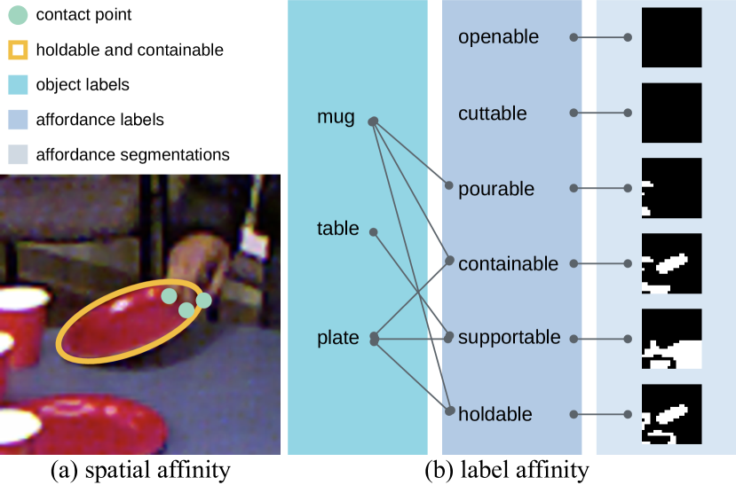
Figure 1: Affordance segmentation with sparse point supervision. (a) Object affordance is usually accessible by human-object interaction with sparse contact points. Propagating such sparse point annotation leverages spatial affinity. (b) Affordance is inherently multi-label [18]: A plate can be both holdable and containable, thus possessing label affinity. By leveraging this dual affinity connecting low- and high-level image cues, we address affordance segmentation as a multi-label dense prediction problem.

In this work, we demonstrate how point supervision promotes affordance segmentation by leveraging a dual affinity that connects the low- and high-level cues in images:

• Dense affordance labels can arise from sparse point annotation by spatial affinity. Take Fig. 1 for an example. We can assign dense labels of holdable to the entire plate by observing a person holding it with sparse contact points. Computationally, we can obtain sparse point annotations for the holdable label by predicting the hold label (action recognition) and determining the contact points between the hand and the plate (3D hand-object interaction, such as prior arts [6, 50]). Since the plate has a uniform color, we can propagate the sparse holdable label from those points to the entire plate.

• Unlike conventional image segmentation, affordance is inherently multi-label [18]; for instance, a plate is both holdable and containable. This unique nature of affordance touches uncharted territory in pointly-supervised segmentation: label affinity.

Leveraging the above unique properties introduced by dual affinity, we devise an end-to-end architecture for affordance segmentation, named Structured TRansformer for Affordance Segmentation with Point Supervision, or STRAP for short. To tackle label affinity, we attach a recurrent network that models pixel-wise label relations onto conventional dense prediction networks; this design allows us to densify sparse affordance labels in label space. Our recipe for spatial affinity includes two essential ingredients. The first is a Transformer backbone that models global patch interaction with self-attention, such that the long-range affinity among patches is implicitly learned. The second is a regularization loss that encourages spatially coherent predictions aligned with low-level cues.

This work makes three contributions:

• To our best knowledge, ours is the first that proposes the concept of dual affinity for affordance segmentation. Our experimental results demonstrate the efficacy of this idea.

• To our best knowledge, ours is the first to model label affinity for learning multi-label affordance segmentation with point-level sparse annotation.

• Our modeling of spatial affinity using a Transformer backbone and a regularization loss results in a compact end-to-end architecture structured in two dimensions.

2 Related work

Affordance

The concept of affordance [18] refers to an object’s capability to support a specific action, which also relates to the concept of functionality [63, 65, 48, 27, 33]; we refer the readers to a recent survey [21]. Research on affordance can be roughly categorized into three focuses. The first is scene affordance; the core idea is to fit the human skeleton or activities to the observed scenes [15, 19], either by geometry [23, 35] or contact force [67]. Modern treatments leverage large-scale datasets by sitcoms [58] or self-collected egocentric videos [44]. Ultimately, the goal of scene affordance is to provide valuable cues for holistic scene understanding tasks [30, 25, 7, 36, 26]. The second is object affordance detection [66]. With benchmark [10], prior arts [43, 53, 55, 5] regard affordance as a dense prediction task and resolve it under pixel-level supervision. The third is affordance emerged from human-object interactions [60, 68, 47, 42, 29], providing interaction cues for planning and acting [13, 12, 62, 16, 64, 20]. Recently, this direction has been further extended to generative models that directly synthesize interactions from observation [3, 28, 39, 34, 59, 24]. Compared to the literature, our work addresses affordance through interactions in a pointly-supervised fashion at the pixel level, providing a trade-off between data efficiency and model performance.

Pointly-supervised learning

Since dense annotation is expensive and time-consuming [52], the pointly-supervised approach provides a natural and effective way for weak annotation. Point supervision for semantic segmentation was first introduced [1] for PASCAL VOC 2012 dataset [14]. Some notable work includes extreme points with point-centric Gaussian channel [40], a distance metric loss leveraging semantic relations among annotated points [49], a point annotation scheme for uniform sampling, and applications in panoptic segmentation [41, 37]. In this work, we leverage the same idea of sparse point supervision for affordance segmentation.

3 Method

Problem definition

We formulate affordance segmentation as a multi-label dense prediction task. We assume image $X$ contains one or more objects, and the ground-truth labels $Y$ are given by sparse point annotations to roughly locate the affordance regions. Formally, an image $X\in\mathbb{R}^{H\times W\times 3}$ has binary ground-truth labels $Y=\{y_{i}\mid y_{i}\in\mathbb{R}^{H\times W\times 1}\}$, where $y_{i}$ denotes the affordance label for one certain action .

The dual affinity property

With only rough localizations for affordance regions, point supervision cannot accurately delineate the boundary of an affordance region. To tackle this challenge, we exploit a unique dual affinity property in affordance segmentation to compensate for the sparsity of $Y$. Specifically, spatial affinity (see Sec. 3.2) is the pixel similarity in terms of visual properties and positions, potentially providing additional cues to alleviate the sparsity of $Y$. Meanwhile, label affinity (see Sec. 3.3) is the structured relation between object labels and affordance labels; proper modeling of this latent space mitigates the imbalance introduced by both the sparsity of $Y$ and the long-tailed dataset. Computationally, we model the dual affinity with a recurrent network (label affinity) and a regularization loss (spatial affinity).

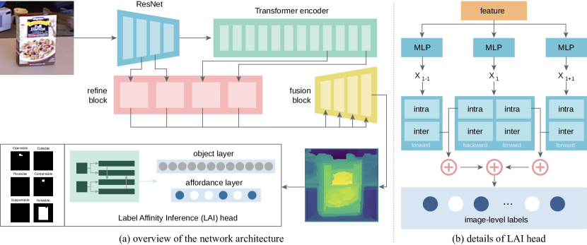
Figure 2: Network architecture and the label affinity inference (LAI) head. (a) A query image is first fed into a ResNet to extract features. Next, the feature embeddings with a position embedding are passed through Transformer encoders as tokens, reassembled from ResNet and Transformer encoders; these tokens are processed by refine blocks. Finally, a sequence of fusion blocks progressively fuses and upsamples these tokens to the image-like representations; features generated from the last fusion block are used for dense prediction and LAI. (b) Fully connected layers are adopted to project the given features into label affinity space, with each layer modeling the inter-relations (between affordance and object classes) and intra-relations (among different affordance classes). All label predictions in each layer are generated by a combination of top-down and bottom-up inference, and each of these inferences is a combination of inter- and intra-relations.

3.1 Network architecture

The long-range dependency of Transformer-based attention mechanism is suitable for weakly-supervised methods in many applications [5, 17, 57]. In this work, we exploit a Transformer backbone with a group of dense prediction heads in a pointly-supervised manner for affordance segmentation. Specifically, we design a label affinity inference (LAI) head to model the correlations between object labels and affordance labels, pointly-supervised by human interactions with objects in daily activities. Notably, labels yielded by human interactions with objects are sparse in nature; furthermore, they differ from individuals when interacting with objects or annotating ground-truth labels. Hence, the crux of point supervision is to establish and leverage the accumulated experiences to build up the co-occurrence, therefore densifying the labels. Fig. 2a shows network architecture.

Transformer backbone

We follow the definitions and designs introduced by prior arts [5, 51]. First, an input image $X$ is divided into $N_{p}=\frac{HW}{p^{2}}$ non-overlapping patches of size $p^{2}$ ($p=16$ in our settings); We transform the list of these patches into a vector of 2-D patches. A ResNetV2-50 backbone [22] is adopted to extract feature maps as tokens (blue $\blacksquare$ in Fig. 2’s top left panel). Next, a learnable position embedding is concatenated to retain spatial information. Similar to the modern vision transformer designs [11, 51, 4], a special token is added to gain global information, termed the readout token. Finally, the network generates $N_{p}+1$ tokens $\{t_{0},t_{1},\dots,t_{N_{p}}\}$, where $t_{0}$ is the readout token. All tokens are then encoded by a sequence of multi-head self-attention blocks (green $\blacksquare$ in Fig. 2’s top left panel).

To reassemble the tokens from four different layers: the first and the second stage from ResNetV2-50 backbone, and the 9th and the 12th layers from Transformer encoders (red $\blacksquare$ in Fig. 2’s top left panel), we design a three-stage procedure to restore the image-like representations for tokens from Transformer encoders:

1. We use a projection block to fuse the readout token $t_{0}$ into other tokens. The projection block is defined as

   $$\small\mathrm{token_{proj}}(t_{i})=\mathrm{GELU}\left(\mathrm{MLP}\left(\mathrm{Concat}(t_{i},t_{0})\right)\right),$$ (1)

   where $i=1,2,\dots,N_{p}$.

2. After projection, the new $N_{p}$ tokens are reshaped into image-like representations from $\mathbb{R}^{N_{p}\times D}$ to $\mathbb{R}^{\frac{H}{p}\times\frac{W}{p}\times D}$ by a spatial rearrangement operation.

3. We use a $1\times 1$ and a $3\times 3$ convolution to resample features from $\mathbb{R}^{\frac{H}{p}\times\frac{W}{p}\times D}$ to $\mathbb{R}^{\frac{H}{s}\times\frac{W}{s}\times\hat{D}}$, where $s>p$.

To fuse these extracted tokens, we use RefineNet-based fusion blocks [38] to upsample them progressively (yellow $\blacksquare$ in Fig. 2’s top left panel). Besides the first block, each fusion block processes the output of the previous fusion block and the related extracted token together, and the resolution of the final feature representation $F$ will be upsampled into $\mathbb{R}^{\frac{H}{2}\times\frac{W}{2}\times\hat{D}}$. The final feature representation $F$ is used for dense prediction and LAI.

Dense prediction head

The dense prediction head leverages two components to generate affordance segmentation: fully connected layers to generate the affordance map and a bilinear interpolation function to restore the resolution of the affordance map to the original resolution of $X$. As such, the size of its output is upsampled into $H\times W\times 1$.

Usually, the binary cross-entropy loss is a well-behaved choice in full supervision. However, as the foreground pixel number and background pixel number are imbalanced in point supervision, we adopt a partial binary cross-entropy (PCE) loss as the dense prediction objective, whose effectiveness is supported by the ablation studies in Tab. 2:

$$\mathcal{L}_{\mathrm{PCE}}\left(\hat{Y},Y\right) =\frac{1}{|\mathrm{fg}|}\sum_{y\in Y,\hat{y}\in\hat{Y}}{y\log{\left(\hat{y}\right)}}$$ (2)

$$+\frac{1}{|\mathrm{bg}|}\sum_{y\in Y,\hat{y}\in\hat{Y}}{\left(1-y\right)\log{\left(1-\hat{y}\right)}},$$

where $|\mathrm{fg}|$ is the number of foreground pixels, $|\mathrm{bg}|$ is the number of background pixels, $Y$ is the ground-truth labels, and $\hat{Y}$ are the outputs of dense prediction heads activated by a sigmoid function. This PCE technique is inspired by the influential edge detection method HED [61].

3.2 Spatial affinity

Spatial affinity is the pixel similarity in terms of visual properties and positions. As point annotations are sparse in nature, they are inadequate to provide sufficient information to determine the shape of the affordance region. Hence, an auxiliary method is in need.

Intuitively, the point annotations of affordance could be propagated to visual regions with similar colors and nearby positions, sharing the same spirit of image segmentations. Modern treatments using conditional random field (CRF) loss [32, 56, 46] can fill this gap between point supervision and full supervision. In particular, sparse-connected CRF loss [56] has demonstrated similar performance while avoiding the time-consuming process in the dense-connected CRF loss.

First, we define the kernel as:

$$\small K_{ab}=\sum_{p=1}^{P}{w^{\left(p\right)}\cdot\exp{\left\{-\frac{1}{2}\left|\frac{f_{a}^{\left(p\right)}-f_{b}^{\left(p\right)}}{\sigma^{\left(p\right)}}\right|^{2}\right\}}},$$ (3)

where $K_{ab}$ is the weighted sum of $P$ kernels, $w^{\left(p\right)}$ is the weight of kernel $p$, $\sigma^{\left(p\right)}$ is a hyperparameter to control the $\mathrm{p^{th}}$ kernel’s bandwidth, and $f_{a}^{\left(p\right)}$ ($f_{b}^{\left(p\right)}$) is the value of kernel-specific feature vector at position $a$ ($b$).

Next, we calculate the weighted sum of kernels at the position pair $(a,b)$:

$$\psi_{a,b}\left(\hat{Y}\right) =\sum_{i,j\in\left[1,C\right]}{\mu\left(i,j\right)\cdot\hat{y}_{a}\left(i\right)\cdot\hat{y}_{b}\left(j\right)\cdot K_{ab}},$$ (4)

$$\mu\left(i,j\right) =\left\{\begin{array}[]{ll}0,\quad{}\text{ if }i=j\\ 1,\quad{}\text{ otherwise }\end{array}\right.,$$

where $\mu\left(i,j\right)\cdot\hat{y}_{a}\left(i\right)\cdot\hat{y}_{b}\left(j\right)$ is a relaxed Potts model of class compatibility, and $C$ is the number of affordance classes in the dataset (Here $C=2$ as we apply the CRF loss on foreground and background separately.).

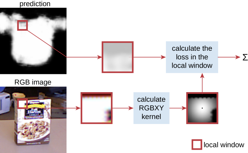
Figure 3: Spatial loss by CRF. First, a local window slides from the top left to the bottom right to generate a sequence of RGBXY kernels, which are later merged with position information. Next, a similar operation divides the foreground and background predictions into patches, whose size equals the kernels’. Finally, the total loss is the sum of the losses on all local windows.

Finally, we use an RGBXY kernel to capture the color similarity and position proximity by CRF:

$$\small\mathcal{L}_{\mathrm{spatial}}\left(\hat{Y},X\right)=\frac{1}{N}\sum_{a=1}^{N}{\sum_{b\in\Omega_{r}\left(a\right)\setminus\left\{a\right\}}{\psi_{a,b}\left(\hat{Y}\right)}},$$ (5)

where $N$ is the total number of pixels, and $\Omega_{r}\left(a\right)$ denotes a sliding window at $\left[a_{x}-r,a_{x}+r\right]\times\left[a_{y}-r,a_{y}+r\right]$; $r$ is the half-width of the slide window. All feature vectors (i.e., RGBXY kernel vectors) are generated by the image $X$, the position matrix, and the binary dense prediction $\hat{Y}$. Fig. 3 illustrates the spatial loss of a sliding window using CRF.

3.3 Label affinity

Label affinity is the structured relation between object labels and affordance labels. We devise the label affinity to model two essential relations: (i) an intra-relation that models the relations between different affordance classes and the relations between different objects, and (ii) an inter-relation that models the relation between affordance and object classes. Fig. 2b illustrates this LAI head. Similar to the prior design [45], we leverage a bidirectional recurrent neural network to model label affinity. The module comprises two label layers: the implicit object layer and the explicit affordance layer. We model the inter-relation across the label layers and the intra-relation in each label layer. Each layer outputs the probability of labels activated by a sigmoid function, and the whole structure is defined as a directed graph.

First, the input feature $x_{l}$ is fed into label layer $l$,

$$\small x_{l}=F_{\mathrm{flatten}}W_{F,l}^{\mathrm{T}}+b_{F,l},$$ (6)

where $l$ is the index of the current layer, $n_{l}$ is the number of classes in layer $l$, $W_{F,l}\in\mathbb{R}^{n_{l}\times C}$ and $b_{F,l}\in\mathbb{R}^{1\times n_{l}}$ are learnable parameters, and $F_{\mathrm{flatten}}\in\mathbb{R}^{1\times C}$ is a flattened vector of the Transformer backbone’s final feature representation $F\in\mathbb{R}^{\frac{H}{2}\times\frac{W}{2}\times\hat{D}}$.

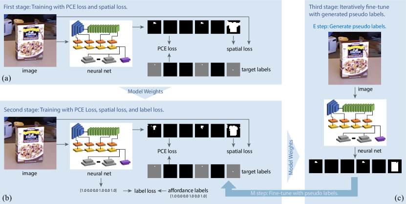
Figure 4: Our multi-stage training strategy. (a) In the first stage, we train our network with the PCE loss and the spatial loss supervised by point annotations. (b) In the second stage, the LAI head is added to fine-tune the network by modeling the intra- and inter-relations. This stage is jointly trained by the PCE loss, the spatial loss, and the label loss. (c) In the third stage, we use the EM algorithm [9] to generate pseudo labels (E step) and fine-tune the network (M step) iteratively.

Next, to output the probabilities of each label, we use a combination of the result of top-down inference $\overrightarrow{f}_{l}$ and the result of bottom-up inference $\overleftarrow{f}_{l}$, conceptually illustrated in Fig. 2b:

$$\overrightarrow{f}_{l} =\overrightarrow{f}_{l-1}\cdot\overrightarrow{W}_{\mathrm{inter},l}^{T}+x_{l}\cdot\overrightarrow{W}_{\mathrm{intra},l}^{T}+\overrightarrow{b}_{l},$$ (7)

$$\overleftarrow{f}_{l} =\overleftarrow{f}_{l+1}\cdot\overleftarrow{W}_{\mathrm{inter},l}^{T}+x_{l}\cdot\overleftarrow{W}_{\mathrm{intra},l}^{T}+\overleftarrow{b}_{l},$$

$$f_{l} =\overrightarrow{f}_{l}\cdot\overrightarrow{W}_{l}^{T}+\overleftarrow{f}_{l}\cdot\overleftarrow{W}_{l}^{T}+b_{l},$$

where $W_{\mathrm{inter}}$ denotes the weight of inter-relation, and $W_{\mathrm{intra}}$ denotes the weight of intra-relation. We generate image-level affordance labels $Z\in\mathbb{R}^{n\times 1}$ by point annotations, where $n$ is the number of affordance classes. Hence, we can use a binary cross-entropy loss to optimize this module:

$$\mathcal{L}_{\mathrm{label}}\left(\hat{Z},Z\right) =\frac{1}{n}\sum_{z\in Z,\hat{z}\in\hat{Z}}{z\cdot\log{\left(\hat{z}\right)}}$$ (8)

$$+\frac{1}{n}\sum_{z\in Z,\hat{z}\in\hat{Z}}{\left(1-z\right)\cdot\log{\left(1-\hat{z}\right)}},$$

where $n$ is the number of labels in the last layer (it’s equal to the number of affordance classes in our settings), $Z$ is the ground-truth label, and $\hat{Z}$ is the output of the last layer activated by a sigmoid function.

3.4 Training

Objective

Given sparse point annotations, training requires converting them to image-like pseudo labels $Y$ as shown in prior work [55, 54]:

$$\small Y\left(i,j\right)=\left\{\begin{array}[]{ll}1,&\text{if }\left(i-p^{k}_{i}\right)^{2}+\left(j-p^{k}_{j}\right)^{2}<\sigma_{\mathrm{d}}\\ 0,&\text{otherwise}\end{array}\right.,$$ (9)

where $\left(i,j\right)$ denotes the 2-D position of $Y$, $\left(p^{k}_{i},p^{k}_{j}\right)$ denotes the 2-D position of the $k^{\mathrm{th}}$ point annotation, and $\sigma_{\mathrm{d}}$ is a hyperparameter that controls the size of pseudo patterns. Of note, setting $\sigma_{\mathrm{d}}>1$ [54] is equivalent to increasing the number of the point annotations, facilitating the feature learning of affordance regions; this introduces an effect akin to the spatial affinity. However, such dilation of point annotations also introduces undesirable artifacts in local regions with intricate boundaries. Hence, in this work, we set $\sigma_{\mathrm{d}}=1\mathrm{px}$ to ensure the correctness of $Y$.

Table 1: Comparisons between our methods and prior methods on the object split and the actor split.

	methods	openable$\uparrow$	cuttable$\uparrow$	pourable$\uparrow$	containable$\uparrow$	supportable$\uparrow$	holdable$\uparrow$	mIoU$\uparrow$
object split	WTP [1]	0.01	0.00	0.09	0.02	0.03	0.19	0.06
	Johann Sawatzky et al. [55]	0.11	0.09	0.21	0.28	0.36	0.56	0.27
	Johann Sawatzky et al. [54]	0.15	0.21	0.37	0.45	0.61	0.54	0.39
	Ours	0.52	0.49	0.55	0.57	0.57	0.65	0.60
actor split	WTP [1]	0.13	0.00	0.08	0.10	0.11	0.22	0.11
	Johann Sawatzky et al. [55]	0.23	0.14	0.28	0.33	0.24	0.42	0.27
	Johann Sawatzky et al. [54]	0.50	0.00	0.39	0.43	0.64	0.56	0.42
	Ours	0.34	0.07	0.40	0.40	0.49	0.59	0.46

Training strategy

We devise a three-stage training strategy to fully unleash the power of dual affinity modeling; see Fig. 4. Our training strategy is efficient: We directly use $Y$ in the first/second stage and further refine $Y$ without time-consuming post-processing in the third stage.

In the first stage, we only use the PCE loss Eq. 2 and the spatial loss Eq. 5 to train our network; the total loss is:

$$\small\mathcal{L}_{\mathrm{s1}}=\lambda_{1}\mathcal{L}_{\mathrm{PCE}}+\lambda_{2}\mathcal{L}_{\mathrm{spatial}},$$ (10)

where $\lambda_{1}=1$, and $\lambda_{2}=0.1$ in our settings.

In the second stage, we add the LAI head to exploit the inter-/intra-relations and only use the image-level affordance labels Eq. 8 to supervise the LAI head. The total loss is:

$$\small\mathcal{L}_{\mathrm{s2}}=\lambda_{1}\mathcal{L}_{\mathrm{PCE}}+\lambda_{2}\mathcal{L}_{\mathrm{spatial}}+\lambda_{3}\mathcal{L}_{\mathrm{label}},$$ (11)

where $\lambda_{1}=1$, $\lambda_{2}=0.1$, and $\lambda_{3}=1$ in our settings. This strategy eases the training of LAI head.

In the third stage, we adopt the expectation–maximization (EM) algorithm to boost the network performance progressively without any post-processing trick to refine pseudo labels (e.g., dense CRF inference [32]). The iteration of EM includes two steps: (i) In the E step, we freeze our network to predict the affordance maps and use the flood-fill algorithm to extract all foreground regions annotated by sparse point annotations. (ii) In the M step, we train our network supervised by these pseudo labels and affordance labels, with the same total loss as in Eq. 11.

Flood-fill algorithm

Flood fill is an algorithm that propagates the connected and similarly-colored region from the initial nodes; i.e., the point annotations in our settings. We only use the connectivity for flooding since the affordance segmentation yields a set of binary maps. There are two common strategies to find eligible adjacent nodes: four-way (in the shape of a cross) and eight-way (in the shape of a rectangle). The implementation of the flood-fill algorithm is usually by a stack- or a queue-based search, wherein the procedure is similar to the depth-first search in a graph. Alg. 1 sketches the pseudocode of the flood-fill algorithm.

Input: $p$: one of the sparse point annotations
$\hat{Y}$: the binary prediction

Output: $Y$: the processed binary prediction

Data: $Q$: an empty queue

1 begin

2       $Y\leftarrow\mathbf{0}$;

3       $Q\leftarrow\textnormal{{push(}}\textnormal{\emph{p}}\textnormal{{)}}$;

4       while $Q$ is not empty do

5             $p_{\mathrm{new}}\leftarrow$ pop($Q$);

6             if $\hat{Y}({p_{\mathrm{new}}})=0$ then

7                   continue;

8                  

9            $Y(p_{\mathrm{new}})\leftarrow 1$;

10             foreach $p_{\mathrm{neighbor}}$ in neighbor($p_{\mathrm{new}}$) do

11                   $Q\leftarrow$ push($p_{\mathrm{neighbor}}$);

12                  

13            

14      

15

Algorithm 1 Flood-fill Algorithm

4 Experiments

We evaluate our methods on the CAD120 dataset [31], which contains two splits: (i) Object split, with no same central object class between the training and the test data. (ii) Actor split, with no same video actor between the training and the test data. Note that the actor split is much more difficult than the object split for all methods inspected, because of scene context domain gap. For evaluation metrics, we adopt the mean intersection-over-union (mIoU) to compare our method’s performance with prior methods.

Implementation details

On each dataset split, we train our network with a batch size of 4 and an initial learning rate $\mathrm{lr}_{\mathrm{init}}$ of 0.001. We use the function $\mathrm{lr}=\mathrm{lr}_{\mathrm{init}}\times\left(1-\frac{\mathrm{epoch}}{100}\right)^{0.9}$ to decay the learning rate during training, with an SGD optimizer with a momentum of 0.9 and a weight decay of 0.0001. In the first and the second stages, given the sparse point supervision (in fact, one point per annotation), we draw disks (i.e., set $\sigma_{\mathrm{d}}=1$px) centered on the point annotation positions to generate pseudo labels, which are used to train our network. In the third stage, we use the predictions in the E step to update the pseudo labels. Every stage lasts 100 epochs. Besides, we apply the EM algorithm every 10 epochs in the third stage, accounting to 10 EM rounds.

\begin{overpic}[width=86.72267pt]{qualitative_results/a/pce_openable}\put(0.0,105.0){\small\color[rgb]{0,0,0}{only \acs{pce} loss}} \put(-20.0,12.0){\rotatebox{90.0}{\color[rgb]{0,0,0}{openable}}} \end{overpic}

\begin{overpic}[width=86.72267pt]{qualitative_results/a/pce+crf_20_0.01_openable}\put(15.0,105.0){\small\color[rgb]{0,0,0}{first stage}} \end{overpic}

\begin{overpic}[width=86.72267pt]{qualitative_results/a/hc_refine_openable}\put(2.0,105.0){\small\color[rgb]{0,0,0}{second stage}} \end{overpic}

\begin{overpic}[width=86.72267pt]{qualitative_results/a/em_openable}\put(15.0,105.0){\small\color[rgb]{0,0,0}{third stage}} \end{overpic}

\begin{overpic}[width=86.72267pt]{qualitative_results/a/gt_openable}\put(2.0,105.0){\small\color[rgb]{0,0,0}{ground truth}} \end{overpic}

\begin{overpic}[width=86.72267pt]{qualitative_results/a/pce_containable}\put(-20.0,2.0){\rotatebox{90.0}{\color[rgb]{0,0,0}{containable}}} \end{overpic}

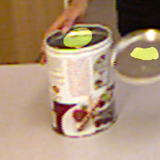
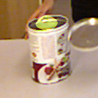
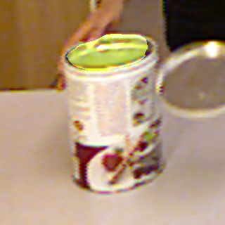
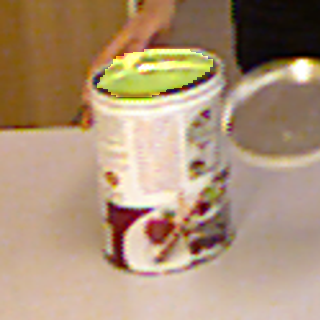
\begin{overpic}[width=86.72267pt]{qualitative_results/a/pce_holdable}\put(-20.0,15.0){\rotatebox{90.0}{\color[rgb]{0,0,0}{holdable}}} \end{overpic}

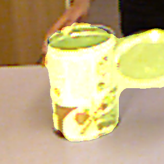
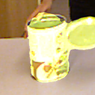
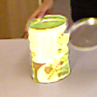
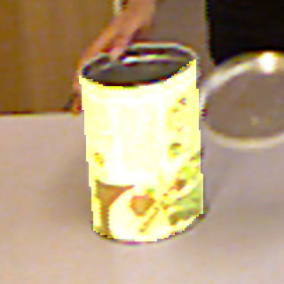
(a)

\begin{overpic}[width=86.72267pt]{qualitative_results/b/pce_pourable}\put(0.0,105.0){\small\color[rgb]{0,0,0}{only \acs{pce} loss}} \put(-20.0,12.0){\rotatebox{90.0}{\color[rgb]{0,0,0}{pourable}}} \end{overpic}

\begin{overpic}[width=86.72267pt]{qualitative_results/b/pce+crf_20_0.01_pourable}\put(15.0,105.0){\small\color[rgb]{0,0,0}{first stage}} \end{overpic}

\begin{overpic}[width=86.72267pt]{qualitative_results/b/hc_refine_pourable}\put(2.0,105.0){\small\color[rgb]{0,0,0}{second stage}} \end{overpic}

\begin{overpic}[width=86.72267pt]{qualitative_results/b/em_pourable}\put(15.0,105.0){\small\color[rgb]{0,0,0}{third stage}} \end{overpic}

\begin{overpic}[width=86.72267pt]{qualitative_results/b/gt_pourable}\put(2.0,105.0){\small\color[rgb]{0,0,0}{ground truth}} \end{overpic}

\begin{overpic}[width=86.72267pt]{qualitative_results/b/pce_containable}\put(-20.0,2.0){\rotatebox{90.0}{\color[rgb]{0,0,0}{containable}}} \end{overpic}

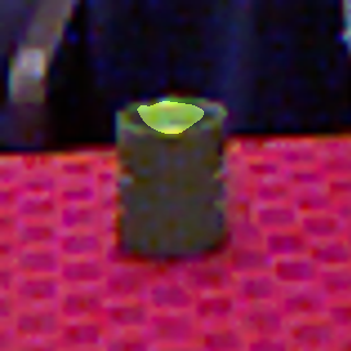
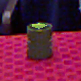
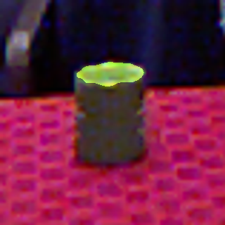
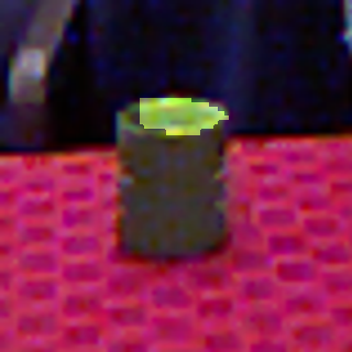
\begin{overpic}[width=86.72267pt]{qualitative_results/b/pce_holdable}\put(-20.0,15.0){\rotatebox{90.0}{\color[rgb]{0,0,0}{holdable}}} \end{overpic}

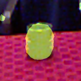
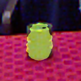
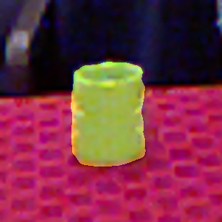
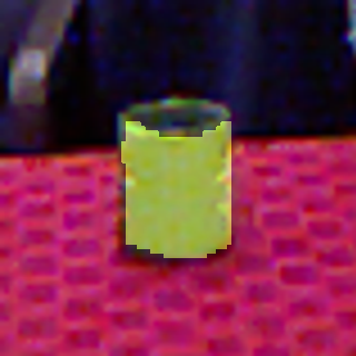
(b)

\begin{overpic}[width=86.72267pt]{qualitative_results/c/pce_openable}\put(-20.0,12.0){\rotatebox{90.0}{\color[rgb]{0,0,0}{openable}}} \end{overpic}

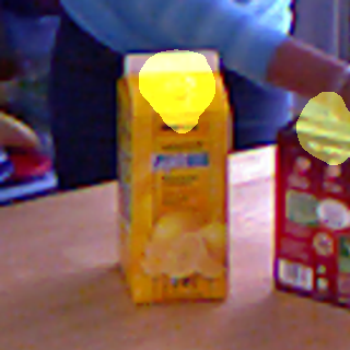
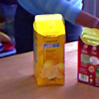
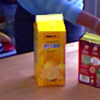
\begin{overpic}[width=86.72267pt]{qualitative_results/c/pce_containable}\put(-20.0,2.0){\rotatebox{90.0}{\color[rgb]{0,0,0}{containable}}} \end{overpic}

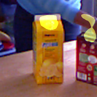
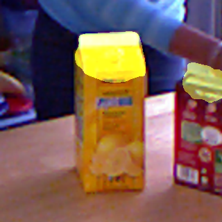
\begin{overpic}[width=86.72267pt]{qualitative_results/c/pce_holdable}\put(-20.0,15.0){\rotatebox{90.0}{\color[rgb]{0,0,0}{holdable}}} \end{overpic}

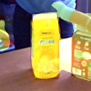
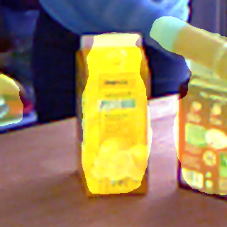
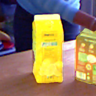
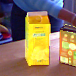
(c)

\begin{overpic}[width=86.72267pt]{qualitative_results/d/pce_openable}\put(-20.0,12.0){\rotatebox{90.0}{\color[rgb]{0,0,0}{openable}}} \end{overpic}

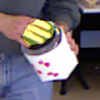
\begin{overpic}[width=86.72267pt]{qualitative_results/d/pce_containable}\put(-20.0,2.0){\rotatebox{90.0}{\color[rgb]{0,0,0}{containable}}} \end{overpic}

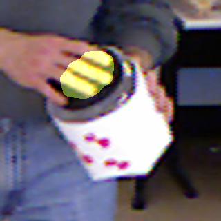
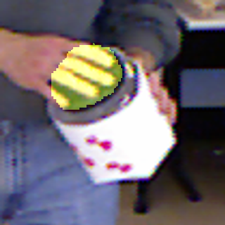
\begin{overpic}[width=86.72267pt]{qualitative_results/d/pce_holdable}\put(-20.0,15.0){\rotatebox{90.0}{\color[rgb]{0,0,0}{holdable}}} \end{overpic}

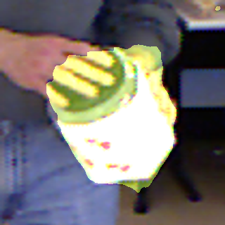
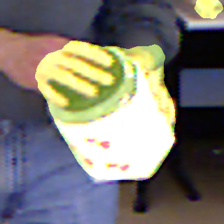
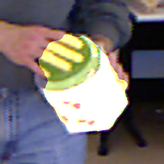
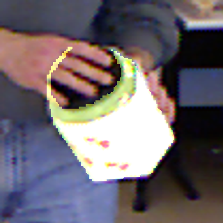
(d)

Figure 5: Qualitative results in three different affordance classes.

Table 2: Ablations of our methods on the object spit and the actor split.

	PCE	spatial affinity	label affinity	EM	openable$\uparrow$	cuttable$\uparrow$	pourable$\uparrow$	containable$\uparrow$	supportable$\uparrow$	holdable$\uparrow$	mIoU$\uparrow$
object split	✓				0.39	0.59	0.33	0.37	0.64	0.38	0.41
	✓	✓			0.44	0.45	0.49	0.50	0.57	0.48	0.49
	✓	✓	✓		0.55	0.49	0.50	0.55	0.58	0.52	0.53
	✓	✓	✓	✓	0.52	0.49	0.55	0.57	0.57	0.65	0.60
actor split	✓				0.27	0.05	0.37	0.34	0.50	0.37	0.37
	✓	✓			0.21	0.01	0.41	0.35	0.48	0.47	0.39
	✓	✓	✓		0.26	0.00	0.45	0.39	0.48	0.55	0.44
	✓	✓	✓	✓	0.34	0.07	0.40	0.40	0.49	0.59	0.46

Quantitative results

Our methods outperform the state-of-the-art on both the object split and the actor split in terms of the mIoU by 53.8% and 9.5%, relatively; see Tab. 1. In particular, our method significantly outperforms prior methods in individual affordance classes (except “supportable”) on object split. It is on par with the state-of-the-art methods in individual affordance classes on actor split.

Qualitative results

We visualize four examples as the qualitative results in Fig. 5. Below, we summarize some notable observations in each example.

• Fig. 5(a): The containable region on the lid is eradicated after the second stage, indicating that our methods can restrain the prediction of the unreasonable region when using the label affinity loss in the second stage.

• Fig. 5(b): The pourable region on the mug rim emerges after introducing the label affinity. This result demonstrates the efficacy of our design of label affinity loss.

• Fig. 5(c): Distinguishing different affordance regions with only one point per affordance region is challenging. The spatial affinity loss cannot solve this difficulty, as shown by the prediction of holdable region in the first stage. Again, this challenge is solved by the label affinity loss, which models the intra-relation of object labels.

• Fig. 5(d): Despite being annotated with other affordance classes, the top-right region lacks the point annotation for holdable. Hence, the algorithm struggles in prediction with only PCE loss and the spatial affinity loss. In fact, this label is also challenging for humans due to its small scale, color distortion, and incomplete shape. Yet, our network still discovers the top-right holdable region by introducing the label affinity loss in the second stage.

Ablations of loss functions

We further conduct some ablations of loss functions in our method, summarized in Tab. 2. On object split, we observe a 19.5% performance improvement in mIoU when adding the spatial affinity loss and another 8.2% in mIoU when adding the label affinity loss. These improvements demonstrate that both spatial affinity and label affinity play a central role in filling the gap between full and point supervision. Moreover, without time-consuming post-processing, the EM algorithm brings in a 13.2% performance improvement in mIoU, demonstrating the efficacy of our design. Although we did not observe similar significant improvements on actor split, our design still yields a similar performance or progressively improved performance with additional modules added.

Ablations of $\mathbf{\sigma_{\mathrm{d}}}$

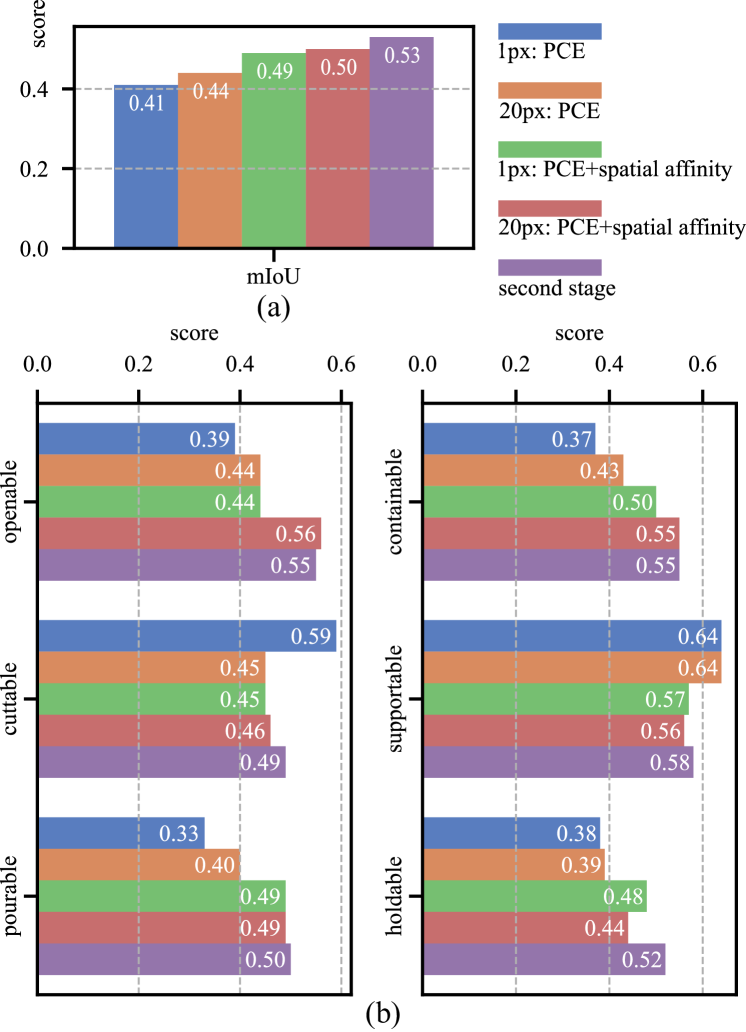
Figure 6: Ablations of $\mathbf{\sigma_{\mathrm{d}}}$. We experiment and compare five settings: (i) PCE loss with $\sigma_{\mathrm{d}}=1\mathrm{px}$, (ii) PCE loss and CRF loss with $\sigma_{\mathrm{d}}=1\mathrm{px}$ (i.e., the first stage), (iii) PCE loss with $\sigma_{\mathrm{d}}=20\mathrm{px}$, (iv) PCE loss and CRF loss with $\sigma_{\mathrm{d}}=20\mathrm{px}$, and (v) the performance obtained up to the second stage in training.

We further ablate a crucial parameter $\sigma_{\mathrm{d}}$. Prior methods suggest that a larger $\sigma_{\mathrm{d}}$ may lead to better performance [54] ($\sigma_{\mathrm{d}}=20\mathrm{px}$). At first glance, this empirical result is echoed by the comparison shown in Fig. 6a. Specifically, we observe that $\sigma_{\mathrm{d}}=20\mathrm{px}$ yields better mIoU compared to $\sigma_{\mathrm{d}}=1\mathrm{px}$ (i) with PCE loss only (the orange vs. the blue) and (ii) with both PCE loss and spatial affinity loss (the red vs. the green). However, our further analysis of individual affordance classes refutes the empirical finding that larger $\sigma_{\mathrm{d}}$ may lead to better performance.

Fig. 6b summarizes the results of individual affordance classes, which presents a mixed picture. For instance, when only using the PCE loss, the mIoU of $\sigma_{\mathrm{d}}=20\mathrm{px}$ is 7.3% higher than $\sigma_{\mathrm{d}}=1\mathrm{px}$; conversely, adding the spatial affinity loss reduces this gap to 2.0%. Overall, only the affordance classes of openable, pourable, and containable indicate $\sigma_{\mathrm{d}}=20\mathrm{px}$ is suitable, whereas the others do not. Interestingly, our proposed LAI head (i.e., the second stage) performs the best among all five conditions, indicating the efficacy of the dual affinity design.

Table 3: The cumulative percentages of a specific $\mathbf{\sigma_{\mathrm{dm}}}$.

affordance class	$<$ 20px	$<$ 50px
openable	14.07%	66.24%
cuttable	57.10%	100.00%
pourable	8.38%	65.54%
containable	12.42%	70.77%
supportable	18.21%	61.38%
holdable	28.09%	67.66%

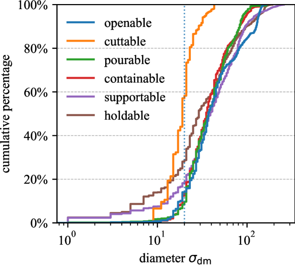
Figure 7: Cumulative percentage curve of $\mathbf{\sigma_{\mathrm{dm}}}$. We compute the appropriate diameter $\sigma_{\mathrm{dm}}$ for each affordance region, defined as the maximal of $\sigma_{\mathrm{d}}$ that ensures the disk generated by it does not exceed the boundary of ground truth.

We further calculate the cumulative percentage of appropriate diameter $\sigma_{\mathrm{dm}}$ for each affordance class; see Fig. 7. Of note, we define the appropriate diameter $\sigma_{\mathrm{dm}}$ for a specific affordance region as the maximal $\sigma_{\mathrm{d}}$, which ensures that the disk drawn by $\sigma_{\mathrm{dm}}$ does not exceed the boundary of the ground-truth region. The cumulative percentage curve accounts for the advantage of $\sigma_{\mathrm{d}}=20\mathrm{px}$ in openable, pourable, and containable since almost all of $\sigma_{\mathrm{dm}}$ is larger than 20px except holdable and cuttable; see also Tab. 3. This result echoes our above analysis of Fig. 6 and confirms that our setting of $\sigma_{\mathrm{d}}=1\mathrm{px}$ is a more practical solution.

Taken together, our ablations of $\mathbf{\sigma_{\mathrm{d}}}$ challenges the prior findings [54]; instead, our experimental results indicate an optimal solution (i.e., $\sigma_{\mathrm{d}}=1\mathrm{px}$) is the best. This contradiction calls for future investments in affordance segmentation and related tasks.

Drawback

The qualitative results in the third stage also reveal a drawback in terms of the generalization of the EM algorithm. Let us take the holdable in Fig. 5(a) and 5(c) as an example. When learning an affordance region without any point annotation (either the unlabelled class in Fig. 5(a) or the missing annotation in the central figure’s top right corner in Fig. 5(c)), the EM algorithm removes this region iteratively. As such, despite the final result matching the ground-truth label, the EM algorithm prevents the method from compensating for incomplete ground-truth annotations.

5 Conclusion

In this work, we focused on affordance segmentation with sparse point supervision and proposed a novel Transformer-based dense prediction network architecture with a dual affinity design. Experiments demonstrate that our method achieves state-of-the-art performance on the challenging CAD120 dataset.

Computationally, our analysis reveals three essential ingredients: (i) Our method can explicitly understand the shape of the affordance region by spatial affinity. (ii) Label affinity implicitly helps to distinguish the class boundary of different affordance regions and discovers other affordance regions even without point annotations. (iii) Filtering the affordance regions by flood-fill guided by point annotations in the EM algorithm can further boost the performance.

Appendix A EM Algorithm

Given an input image $x$ sampled from an underlying distribution, we can use the network, parameterized by $\theta$, to predict the corresponding affordance segmentation $\hat{y}$. The latent code is defined as the pseudo labels $z$ that have a latent relationship with the ground-truth labels $y$. The log-likelihood objective is defined as:

$$\mathcal{L}\left(\theta\right)={\log{p\left(x\mid\theta\right)}}$$ (12)

To solve this maximum likelihood estimation (MLE) problem, we use the EM algorithm by iteratively applying these two steps:

• Expectation (E) step: In the $t$-th E step, we calculate the quantity of $z^{(t)}$ by the following equation:

  $$q\left(\theta\mid\theta^{(t)}\right) =\mathrm{E}_{z\sim p\left(\cdot\mid x,\theta^{(t)}\right)}\left[\log{p\left(x,z\mid\theta\right)}\right]$$ (13)

  $$=\sum_{z\in Z}{p\left(z\mid x,\theta^{(t)}\right)}\log{p\left(x,z\mid\theta\right)}$$

  where $Z$ represents the distribution of the latent code $z$.

• Maximization (M) step: In the $t$-th M step, we use the stochastic gradient descent (SGD) algorithm to find best $\theta$:

  $$\theta^{(t+1)}=\mathrm{argmax}_{\theta}{q\left(\theta\mid\theta^{(t)}\right)}$$ (14)

We provide a brief proof of correctness as follows:

$$\mathcal{L}\left(\theta^{(t+1)}\right)-\mathcal{L}\left(\theta^{(t)}\right)$$ (15)

$$= \log{p\left(x\mid\theta^{(t+1)}\right)}-\log{p\left(x\mid\theta^{(t)}\right)}$$

$$= \sum_{z\in Z}{p\left(z\mid x,\theta^{(t)}\right)\left(\log{\frac{p\left(x,z\mid\theta^{(t+1)}\right)}{p\left(z\mid x,\theta^{(t+1)}\right)}}-\log{\frac{p\left(x,z\mid\theta^{(t)}\right)}{p\left(z\mid x,\theta^{(t)}\right)}}\right)}$$

$$= q\left(\theta^{(t+1)}\mid\theta^{(t)}\right)-q\left(\theta^{(t)}\mid\theta^{(t)}\right)$$

$$-\sum_{z\in Z}{p\left(z\mid x,\theta^{(t)}\right)\log{\frac{p\left(z\mid x,\theta^{(t+1)}\right)}{p\left(z\mid x,\theta^{(t)}\right)}}}$$

For the first term in Eq. 15, since we choose $\theta$ to improve $q\left(\theta\mid\theta^{(t)}\right)$, we can conclude that:

$$q\left(\theta\mid\theta^{(t+1)}\right)\geq q\left(\theta\mid\theta^{(t)}\right)$$ (16)

For the last term in Eq. 15, we use Jensen’s inequality to get the upper bound of it:

$$\sum_{z\in Z}{p\left(z\mid x,\theta^{(t)}\right)\log{\frac{p\left(z\mid x,\theta^{(t+1)}\right)}{p\left(z\mid x,\theta^{(t)}\right)}}}$$ (17)

$$\leq \log{\sum_{z\in Z}{p\left(z\mid x,\theta^{(t)}\right)\frac{p\left(z\mid x,\theta^{(t+1)}\right)}{p\left(z\mid x,\theta^{(t)}\right)}}}$$

$$= \log{\sum_{z\in Z}p\left(z\mid x,\theta^{(t+1)}\right)}$$

$$= 0$$

Thus, Eq. 15 can be transformed into the following inequation:

$$\mathcal{L}\left(\theta^{(t+1)}\right)-\mathcal{L}\left(\theta^{(t)}\right)\geq 0$$ (18)

where we can conclude that the EM algorithm would boost the network performance.

Appendix B More Qualitative Results

We provide more qualitative results to demonstrate the effectiveness of our method; see Fig. 8.

\begin{overpic}[width=69.38078pt]{figures/supp/18/pred_openable.png}\put(25.0,105.0){\small\color[rgb]{0,0,0}{Openable}} \put(-20.0,35.0){\rotatebox{90.0}{\color[rgb]{0,0,0}{Ours}}} \end{overpic}

\begin{overpic}[width=69.38078pt]{figures/supp/18/pred_cuttable.png}\put(28.0,105.0){\small\color[rgb]{0,0,0}{Cuttable}} \end{overpic}

\begin{overpic}[width=69.38078pt]{figures/supp/18/pred_pourable.png}\put(28.0,105.0){\small\color[rgb]{0,0,0}{Pourable}} \end{overpic}

\begin{overpic}[width=69.38078pt]{figures/supp/18/pred_containable.png}\put(20.0,105.0){\small\color[rgb]{0,0,0}{Containable}} \end{overpic}

\begin{overpic}[width=69.38078pt]{figures/supp/18/pred_supportable.png}\put(20.0,105.0){\small\color[rgb]{0,0,0}{Supportable}} \end{overpic}

\begin{overpic}[width=69.38078pt]{figures/supp/18/pred_holdable.png}\put(27.0,105.0){\small\color[rgb]{0,0,0}{Holdable}} \end{overpic}

\begin{overpic}[width=69.38078pt]{figures/supp/18/gt_openable.png}\put(-20.0,40.0){\rotatebox{90.0}{\small\color[rgb]{0,0,0}{GT}}} \end{overpic}

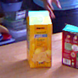
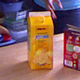
\begin{overpic}[width=69.38078pt]{figures/supp/1/pred_openable.png}\put(-20.0,35.0){\rotatebox{90.0}{\color[rgb]{0,0,0}{Ours}}} \end{overpic}

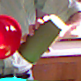
\begin{overpic}[width=69.38078pt]{figures/supp/1/gt_openable.png}\put(-20.0,40.0){\rotatebox{90.0}{\small\color[rgb]{0,0,0}{GT}}} \end{overpic}

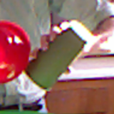
\begin{overpic}[width=69.38078pt]{figures/supp/2/pred_openable.png}\put(-20.0,35.0){\rotatebox{90.0}{\color[rgb]{0,0,0}{Ours}}} \end{overpic}

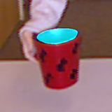
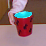
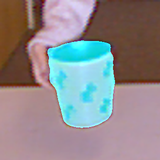
\begin{overpic}[width=69.38078pt]{figures/supp/2/gt_openable.png}\put(-20.0,40.0){\rotatebox{90.0}{\small\color[rgb]{0,0,0}{GT}}} \end{overpic}

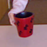
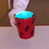
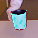
\begin{overpic}[width=69.38078pt]{figures/supp/3/pred_openable.png}\put(-20.0,35.0){\rotatebox{90.0}{\color[rgb]{0,0,0}{Ours}}} \end{overpic}

\begin{overpic}[width=69.38078pt]{figures/supp/3/gt_openable.png}\put(-20.0,40.0){\rotatebox{90.0}{\small\color[rgb]{0,0,0}{GT}}} \end{overpic}

Figure 8: More qualitative results.

\begin{overpic}[width=69.38078pt]{figures/supp/4/pred_openable.png}\put(25.0,105.0){\small\color[rgb]{0,0,0}{Openable}} \put(-20.0,35.0){\rotatebox{90.0}{\color[rgb]{0,0,0}{Ours}}} \end{overpic}

\begin{overpic}[width=69.38078pt]{figures/supp/4/pred_cuttable.png}\put(28.0,105.0){\small\color[rgb]{0,0,0}{Cuttable}} \end{overpic}

\begin{overpic}[width=69.38078pt]{figures/supp/4/pred_pourable.png}\put(28.0,105.0){\small\color[rgb]{0,0,0}{Pourable}} \end{overpic}

\begin{overpic}[width=69.38078pt]{figures/supp/4/pred_containable.png}\put(20.0,105.0){\small\color[rgb]{0,0,0}{Containable}} \end{overpic}

\begin{overpic}[width=69.38078pt]{figures/supp/4/pred_supportable.png}\put(20.0,105.0){\small\color[rgb]{0,0,0}{Supportable}} \end{overpic}

\begin{overpic}[width=69.38078pt]{figures/supp/4/pred_holdable.png}\put(27.0,105.0){\small\color[rgb]{0,0,0}{Holdable}} \end{overpic}

\begin{overpic}[width=69.38078pt]{figures/supp/4/gt_openable.png}\put(-20.0,40.0){\rotatebox{90.0}{\small\color[rgb]{0,0,0}{GT}}} \end{overpic}

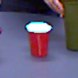
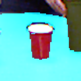
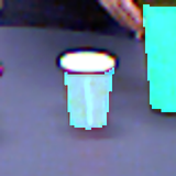
\begin{overpic}[width=69.38078pt]{figures/supp/5/pred_openable.png}\put(-20.0,35.0){\rotatebox{90.0}{\color[rgb]{0,0,0}{Ours}}} \end{overpic}

\begin{overpic}[width=69.38078pt]{figures/supp/5/gt_openable.png}\put(-20.0,40.0){\rotatebox{90.0}{\small\color[rgb]{0,0,0}{GT}}} \end{overpic}

\begin{overpic}[width=69.38078pt]{figures/supp/7/pred_openable.png}\put(-20.0,35.0){\rotatebox{90.0}{\color[rgb]{0,0,0}{Ours}}} \end{overpic}

\begin{overpic}[width=69.38078pt]{figures/supp/7/gt_openable.png}\put(-20.0,40.0){\rotatebox{90.0}{\small\color[rgb]{0,0,0}{GT}}} \end{overpic}

\begin{overpic}[width=69.38078pt]{figures/supp/8/pred_openable.png}\put(-20.0,35.0){\rotatebox{90.0}{\color[rgb]{0,0,0}{Ours}}} \end{overpic}

\begin{overpic}[width=69.38078pt]{figures/supp/8/gt_openable.png}\put(-20.0,40.0){\rotatebox{90.0}{\small\color[rgb]{0,0,0}{GT}}} \end{overpic}

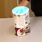
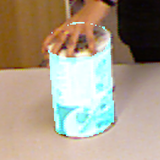
Figure 9: More qualitative results (cont.).

\begin{overpic}[width=69.38078pt]{figures/supp/9/pred_openable.png}\put(25.0,105.0){\small\color[rgb]{0,0,0}{Openable}} \put(-20.0,35.0){\rotatebox{90.0}{\color[rgb]{0,0,0}{Ours}}} \end{overpic}

\begin{overpic}[width=69.38078pt]{figures/supp/9/pred_cuttable.png}\put(28.0,105.0){\small\color[rgb]{0,0,0}{Cuttable}} \end{overpic}

\begin{overpic}[width=69.38078pt]{figures/supp/9/pred_pourable.png}\put(28.0,105.0){\small\color[rgb]{0,0,0}{Pourable}} \end{overpic}

\begin{overpic}[width=69.38078pt]{figures/supp/9/pred_containable.png}\put(20.0,105.0){\small\color[rgb]{0,0,0}{Containable}} \end{overpic}

\begin{overpic}[width=69.38078pt]{figures/supp/9/pred_supportable.png}\put(20.0,105.0){\small\color[rgb]{0,0,0}{Supportable}} \end{overpic}

\begin{overpic}[width=69.38078pt]{figures/supp/9/pred_holdable.png}\put(27.0,105.0){\small\color[rgb]{0,0,0}{Holdable}} \end{overpic}

\begin{overpic}[width=69.38078pt]{figures/supp/9/gt_openable.png}\put(-20.0,40.0){\rotatebox{90.0}{\small\color[rgb]{0,0,0}{GT}}} \end{overpic}

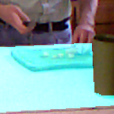
\begin{overpic}[width=69.38078pt]{figures/supp/10/pred_openable.png}\put(-20.0,35.0){\rotatebox{90.0}{\color[rgb]{0,0,0}{Ours}}} \end{overpic}

\begin{overpic}[width=69.38078pt]{figures/supp/10/gt_openable.png}\put(-20.0,40.0){\rotatebox{90.0}{\small\color[rgb]{0,0,0}{GT}}} \end{overpic}

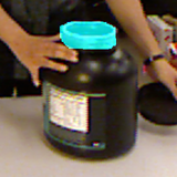
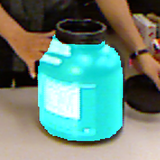
\begin{overpic}[width=69.38078pt]{figures/supp/11/pred_openable.png}\put(-20.0,35.0){\rotatebox{90.0}{\color[rgb]{0,0,0}{Ours}}} \end{overpic}

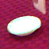
\begin{overpic}[width=69.38078pt]{figures/supp/11/gt_openable.png}\put(-20.0,40.0){\rotatebox{90.0}{\small\color[rgb]{0,0,0}{GT}}} \end{overpic}

\begin{overpic}[width=69.38078pt]{figures/supp/12/pred_openable.png}\put(-20.0,35.0){\rotatebox{90.0}{\color[rgb]{0,0,0}{Ours}}} \end{overpic}

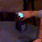
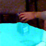
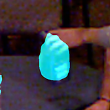
\begin{overpic}[width=69.38078pt]{figures/supp/12/gt_openable.png}\put(-20.0,40.0){\rotatebox{90.0}{\small\color[rgb]{0,0,0}{GT}}} \end{overpic}

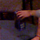
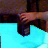
Figure 10: More qualitative results (cont.).

\begin{overpic}[width=69.38078pt]{figures/supp/13/pred_openable.png}\put(25.0,105.0){\small\color[rgb]{0,0,0}{Openable}} \put(-20.0,35.0){\rotatebox{90.0}{\color[rgb]{0,0,0}{Ours}}} \end{overpic}

\begin{overpic}[width=69.38078pt]{figures/supp/13/pred_cuttable.png}\put(28.0,105.0){\small\color[rgb]{0,0,0}{Cuttable}} \end{overpic}

\begin{overpic}[width=69.38078pt]{figures/supp/13/pred_pourable.png}\put(28.0,105.0){\small\color[rgb]{0,0,0}{Pourable}} \end{overpic}

\begin{overpic}[width=69.38078pt]{figures/supp/13/pred_containable.png}\put(20.0,105.0){\small\color[rgb]{0,0,0}{Containable}} \end{overpic}

\begin{overpic}[width=69.38078pt]{figures/supp/13/pred_supportable.png}\put(20.0,105.0){\small\color[rgb]{0,0,0}{Supportable}} \end{overpic}

\begin{overpic}[width=69.38078pt]{figures/supp/13/pred_holdable.png}\put(27.0,105.0){\small\color[rgb]{0,0,0}{Holdable}} \end{overpic}

\begin{overpic}[width=69.38078pt]{figures/supp/13/gt_openable.png}\put(-20.0,40.0){\rotatebox{90.0}{\small\color[rgb]{0,0,0}{GT}}} \end{overpic}

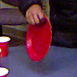
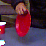
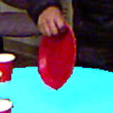
\begin{overpic}[width=69.38078pt]{figures/supp/14/pred_openable.png}\put(-20.0,35.0){\rotatebox{90.0}{\color[rgb]{0,0,0}{Ours}}} \end{overpic}

\begin{overpic}[width=69.38078pt]{figures/supp/14/gt_openable.png}\put(-20.0,40.0){\rotatebox{90.0}{\small\color[rgb]{0,0,0}{GT}}} \end{overpic}

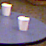
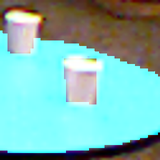
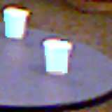
\begin{overpic}[width=69.38078pt]{figures/supp/15/pred_openable.png}\put(-20.0,35.0){\rotatebox{90.0}{\color[rgb]{0,0,0}{Ours}}} \end{overpic}

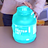
\begin{overpic}[width=69.38078pt]{figures/supp/15/gt_openable.png}\put(-20.0,40.0){\rotatebox{90.0}{\small\color[rgb]{0,0,0}{GT}}} \end{overpic}

\begin{overpic}[width=69.38078pt]{figures/supp/17/pred_openable.png}\put(-20.0,35.0){\rotatebox{90.0}{\color[rgb]{0,0,0}{Ours}}} \end{overpic}

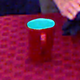
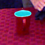
\begin{overpic}[width=69.38078pt]{figures/supp/17/gt_openable.png}\put(-20.0,40.0){\rotatebox{90.0}{\small\color[rgb]{0,0,0}{GT}}} \end{overpic}

Figure 11: More qualitative results (cont.).

\begin{overpic}[width=69.38078pt]{figures/supp/19/pred_openable.png}\put(25.0,105.0){\small\color[rgb]{0,0,0}{Openable}} \put(-20.0,35.0){\rotatebox{90.0}{\color[rgb]{0,0,0}{Ours}}} \end{overpic}

\begin{overpic}[width=69.38078pt]{figures/supp/19/pred_cuttable.png}\put(28.0,105.0){\small\color[rgb]{0,0,0}{Cuttable}} \end{overpic}

\begin{overpic}[width=69.38078pt]{figures/supp/19/pred_pourable.png}\put(28.0,105.0){\small\color[rgb]{0,0,0}{Pourable}} \end{overpic}

\begin{overpic}[width=69.38078pt]{figures/supp/19/pred_containable.png}\put(20.0,105.0){\small\color[rgb]{0,0,0}{Containable}} \end{overpic}

\begin{overpic}[width=69.38078pt]{figures/supp/19/pred_supportable.png}\put(20.0,105.0){\small\color[rgb]{0,0,0}{Supportable}} \end{overpic}

\begin{overpic}[width=69.38078pt]{figures/supp/19/pred_holdable.png}\put(27.0,105.0){\small\color[rgb]{0,0,0}{Holdable}} \end{overpic}

\begin{overpic}[width=69.38078pt]{figures/supp/19/gt_openable.png}\put(-20.0,40.0){\rotatebox{90.0}{\small\color[rgb]{0,0,0}{GT}}} \end{overpic}

\begin{overpic}[width=69.38078pt]{figures/supp/20/pred_openable.png}\put(-20.0,35.0){\rotatebox{90.0}{\color[rgb]{0,0,0}{Ours}}} \end{overpic}

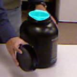
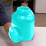
\begin{overpic}[width=69.38078pt]{figures/supp/20/gt_openable.png}\put(-20.0,40.0){\rotatebox{90.0}{\small\color[rgb]{0,0,0}{GT}}} \end{overpic}

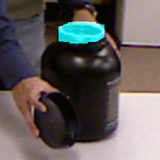
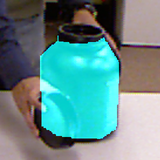
\begin{overpic}[width=69.38078pt]{figures/supp/21/pred_openable.png}\put(-20.0,35.0){\rotatebox{90.0}{\color[rgb]{0,0,0}{Ours}}} \end{overpic}

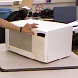
\begin{overpic}[width=69.38078pt]{figures/supp/21/gt_openable.png}\put(-20.0,40.0){\rotatebox{90.0}{\small\color[rgb]{0,0,0}{GT}}} \end{overpic}

\begin{overpic}[width=69.38078pt]{figures/supp/23/pred_openable.png}\put(-20.0,35.0){\rotatebox{90.0}{\color[rgb]{0,0,0}{Ours}}} \end{overpic}

\begin{overpic}[width=69.38078pt]{figures/supp/23/gt_openable.png}\put(-20.0,40.0){\rotatebox{90.0}{\small\color[rgb]{0,0,0}{GT}}} \end{overpic}

Figure 12: More qualitative results (cont.).

References

- [1] Amy Bearman, Olga Russakovsky, Vittorio Ferrari, and Li Fei-Fei. What’s the point: Semantic segmentation with point supervision. In European Conference on Computer Vision (ECCV), 2016.
- [2] Yuri Boykov, Olga Veksler, and Ramin Zabih. Fast approximate energy minimization via graph cuts. Transactions on Pattern Analysis and Machine Intelligence (TPAMI), 23(11):1222–1239, 2001.
- [3] Samarth Brahmbhatt, Ankur Handa, James Hays, and Dieter Fox. Contactgrasp: Functional multi-finger grasp synthesis from contact. In International Conference on Intelligent Robots and Systems (IROS), 2019.
- [4] Mathilde Caron, Hugo Touvron, Ishan Misra, Hervé Jégou, Julien Mairal, Piotr Bojanowski, and Armand Joulin. Emerging properties in self-supervised vision transformers. In International Conference on Computer Vision (ICCV), 2021.
- [5] Xiaoxue Chen, Tianyu Liu, Hao Zhao, Guyue Zhou, and Ya-Qin Zhang. Cerberus transformer: Joint semantic, affordance and attribute parsing. In Conference on Computer Vision and Pattern Recognition (CVPR), 2022.
- [6] Yixin Chen, Siyuan Huang, Tao Yuan, Yixin Zhu, Siyuan Qi, and Song-Chun Zhu. Holistic++ scene understanding: Single-view 3d holistic scene parsing and human pose estimation with human-object interaction and physical commonsense. In International Conference on Computer Vision (ICCV), 2019.
- [7] Yixin Chen, Qing Li, Deqian Kong, Yik Lun Kei, Tao Gao, Yixin Zhu, and Siyuan Huang. Yourefit: Embodied reference understanding with language and gesture. In International Conference on Computer Vision (ICCV), 2021.
- [8] Bowen Cheng, Omkar Parkhi, and Alexander Kirillov. Pointly-supervised instance segmentation. In Conference on Computer Vision and Pattern Recognition (CVPR), 2022.
- [9] Arthur P Dempster, Nan M Laird, and Donald B Rubin. Maximum likelihood from incomplete data via the em algorithm. Journal of the Royal Statistical Society: Series B (Methodological), 39(1):1–22, 1977.
- [10] Shengheng Deng, Xun Xu, Chaozheng Wu, Ke Chen, and Kui Jia. 3d affordancenet: A benchmark for visual object affordance understanding. In Conference on Computer Vision and Pattern Recognition (CVPR), 2021.
- [11] Alexey Dosovitskiy, Lucas Beyer, Alexander Kolesnikov, Dirk Weissenborn, Xiaohua Zhai, Thomas Unterthiner, Mostafa Dehghani, Matthias Minderer, Georg Heigold, Sylvain Gelly, et al. An image is worth 16x16 words: Transformers for image recognition at scale. International Conference on Learning Representations (ICLR), 2021.
- [12] Mark Edmonds, Feng Gao, Hangxin Liu, Xu Xie, Siyuan Qi, Brandon Rothrock, Yixin Zhu, Ying Nian Wu, Hongjing Lu, and Song-Chun Zhu. A tale of two explanations: Enhancing human trust by explaining robot behavior. Science Robotics, 4(37), 2019.
- [13] Mark Edmonds, Feng Gao, Xu Xie, Hangxin Liu, Siyuan Qi, Yixin Zhu, Brandon Rothrock, and Song-Chun Zhu. Feeling the force: Integrating force and pose for fluent discovery through imitation learning to open medicine bottles. In International Conference on Intelligent Robots and Systems (IROS), 2017.
- [14] Mark Everingham, Luc Van Gool, Christopher KI Williams, John Winn, and Andrew Zisserman. The pascal visual object classes (voc) challenge. International Journal of Computer Vision (IJCV), 88(2):303–338, 2010.
- [15] David F Fouhey, Vincent Delaitre, Abhinav Gupta, Alexei A Efros, Ivan Laptev, and Josef Sivic. People watching: Human actions as a cue for single view geometry. In European Conference on Computer Vision (ECCV), 2012.
- [16] Samir Yitzhak Gadre, Kiana Ehsani, and Shuran Song. Act the part: Learning interaction strategies for articulated object part discovery. In International Conference on Computer Vision (ICCV), 2021.
- [17] Huan-ang Gao, Beiwen Tian, Pengfei Li, Xiaoxue Chen, Hao Zhao, Guyue Zhou, Yurong Chen, and Hongbin Zha. From semi-supervised to omni-supervised room layout estimation using point clouds. In International Conference on Robotics and Automation (ICRA), 2023.
- [18] James Jerome Gibson. The ecological approach to visual perception. Houghton, Mifflin and Company, 1979.
- [19] Abhinav Gupta, Scott Satkin, Alexei A Efros, and Martial Hebert. From 3d scene geometry to human workspace. In Conference on Computer Vision and Pattern Recognition (CVPR), 2011.
- [20] Muzhi Han, Zeyu Zhang, Ziyuan Jiao, Xu Xie, Yixin Zhu, Song-Chun Zhu, and Hangxin Liu. Scene reconstruction with functional objects for robot autonomy. International Journal of Computer Vision (IJCV), 2022.
- [21] Mohammed Hassanin, Salman Khan, and Murat Tahtali. Visual affordance and function understanding: A survey. ACM Computing Surveys (CSUR), 54(3):1–35, 2021.
- [22] Kaiming He, Xiangyu Zhang, Shaoqing Ren, and Jian Sun. Deep residual learning for image recognition. In Conference on Computer Vision and Pattern Recognition (CVPR), 2016.
- [23] Siyuan Huang, Siyuan Qi, Yixin Zhu, Yinxue Xiao, Yuanlu Xu, and Song-Chun Zhu. Holistic 3d scene parsing and reconstruction from a single rgb image. In European Conference on Computer Vision (ECCV), 2018.
- [24] Siyuan Huang, Zan Wang, Puhao Li, Baoxiong Jia, Tengyu Liu, Yixin Zhu, Wei Liang, and Song-Chun Zhu. Diffusion-based generation, optimization, and planning in 3d scenes. arXiv preprint arXiv:2301.06015, 2023.
- [25] baoxiong Jia, Yixin Chen, Siyuan Huang, Yixin Zhu, and Song-Chun Zhu. Lemma: A multi-view dataset for learning multi-agent multi-task activities. In European Conference on Computer Vision (ECCV), 2020.
- [26] Baoxiong Jia, Ting Lei, Song-Chun Zhu, and Siyuan Huang. Egotaskqa: Understanding human tasks in egocentric videos. arXiv preprint arXiv:2210.03929, 2022.
- [27] Chenfanfu Jiang, Siyuan Qi, Yixin Zhu, Siyuan Huang, Jenny Lin, Lap-Fai Yu, Demetri Terzopoulos, and Song-Chun Zhu. Configurable 3d scene synthesis and 2d image rendering with per-pixel ground truth using stochastic grammars. International Journal of Computer Vision (IJCV), 126(9):920–941, 2018.
- [28] Hanwen Jiang, Shaowei Liu, Jiashun Wang, and Xiaolong Wang. Hand-object contact consistency reasoning for human grasps generation. In International Conference on Computer Vision (ICCV), 2021.
- [29] Nan Jiang, Tengyu Liu, Zhexuan Cao, Jieming Cui, Yixin Chen, He Wang, Yixin Zhu, and Siyuan Huang. Chairs: Towards full-body articulated human-object interaction. arXiv preprint arXiv:2212.10621, 2022.
- [30] Yun Jiang. Hallucinated Humans: Learning Latent Factors to Model 3D Enviornments. PhD thesis, Cornell University, 2015.
- [31] Hema Swetha Koppula, Rudhir Gupta, and Ashutosh Saxena. Learning human activities and object affordances from rgb-d videos. International Journal of Robotics Research (IJRR), 2013.
- [32] Philipp Krähenbühl and Vladlen Koltun. Efficient inference in fully connected crfs with gaussian edge potentials. In Advances in Neural Information Processing Systems (NeurIPS), 2011.
- [33] Zihang Lai, Senthil Purushwalkam, and Abhinav Gupta. The functional correspondence problem. In International Conference on Computer Vision (ICCV), 2021.
- [34] Puhao Li, Tengyu Liu, Yuyang Li, Yixin Zhu, Yaodong Yang, and Siyuan Huang. Gendexgrasp: Generalizable dexterous grasping. In International Conference on Robotics and Automation (ICRA), 2023.
- [35] Xueting Li, Sifei Liu, Kihwan Kim, Xiaolong Wang, Ming-Hsuan Yang, and Jan Kautz. Putting humans in a scene: Learning affordance in 3d indoor environments. In Conference on Computer Vision and Pattern Recognition (CVPR), 2019.
- [36] Yang Li, Xiaoxue Chen, Hao Zhao, Jiangtao Gong, Guyue Zhou, Federico Rossano, and Yixin Zhu. Understanding embodied reference with touch-line transformer. In International Conference on Learning Representations (ICLR), 2023.
- [37] Yanwei Li, Hengshuang Zhao, Xiaojuan Qi, Yukang Chen, Lu Qi, Liwei Wang, Zeming Li, Jian Sun, and Jiaya Jia. Fully convolutional networks for panoptic segmentation with point-based supervision. Transactions on Pattern Analysis and Machine Intelligence (TPAMI), 2022.
- [38] Guosheng Lin, Anton Milan, Chunhua Shen, and Ian Reid. Refinenet: Multi-path refinement networks for high-resolution semantic segmentation. In Conference on Computer Vision and Pattern Recognition (CVPR), 2017.
- [39] Tengyu Liu, Zeyu Liu, Ziyuan Jiao, Yixin Zhu, and Song-Chun Zhu. Synthesizing diverse and physically stable grasps with arbitrary hand structures using differentiable force closure estimator. IEEE Robotics and Automation Letters (RA-L), 7(1):470–477, 2021.
- [40] Kevis-Kokitsi Maninis, Sergi Caelles, Jordi Pont-Tuset, and Luc Van Gool. Deep extreme cut: From extreme points to object segmentation. In Conference on Computer Vision and Pattern Recognition (CVPR), 2018.
- [41] R Austin McEver and BS Manjunath. Pcams: Weakly supervised semantic segmentation using point supervision. arXiv preprint arXiv:2007.05615, 2020.
- [42] Kaichun Mo, Yuzhe Qin, Fanbo Xiang, Hao Su, and Leonidas Guibas. O2o-afford: Annotation-free large-scale object-object affordance learning. In Conference on Robot Learning (CoRL), 2022.
- [43] Austin Myers, Ching L Teo, Cornelia Fermüller, and Yiannis Aloimonos. Affordance detection of tool parts from geometric features. In International Conference on Robotics and Automation (ICRA), 2015.
- [44] Tushar Nagarajan, Yanghao Li, Christoph Feichtenhofer, and Kristen Grauman. Ego-topo: Environment affordances from egocentric video. In Conference on Computer Vision and Pattern Recognition (CVPR), 2020.
- [45] Nelson Nauata, Hexiang Hu, Guang-Tong Zhou, Zhiwei Deng, Zicheng Liao, and Greg Mori. Structured label inference for visual understanding. Transactions on Pattern Analysis and Machine Intelligence (TPAMI), 42(5):1257–1271, 2019.
- [46] Anton Obukhov, Stamatios Georgoulis, Dengxin Dai, and Luc Van Gool. Gated crf loss for weakly supervised semantic image segmentation. arXiv preprint arXiv:1906.04651, 2019.
- [47] Siyuan Qi, Wenguan Wang, Baoxiong Jia, Jianbing Shen, and Song-Chun Zhu. Learning human-object interactions by graph parsing neural networks. In European Conference on Computer Vision (ECCV), 2018.
- [48] Siyuan Qi, Yixin Zhu, Siyuan Huang, Chenfanfu Jiang, and Song-Chun Zhu. Human-centric indoor scene synthesis using stochastic grammar. In Conference on Computer Vision and Pattern Recognition (CVPR), 2018.
- [49] Rui Qian, Yunchao Wei, Honghui Shi, Jiachen Li, Jiaying Liu, and Thomas Huang. Weakly supervised scene parsing with point-based distance metric learning. In AAAI Conference on Artificial Intelligence (AAAI), 2019.
- [50] Shuwen Qiu, Hangxin Liu, Zeyu Zhang, Yixin Zhu, and Song-Chun Zhu. Human-robot interaction in a shared augmented reality workspace. In International Conference on Intelligent Robots and Systems (IROS), 2020.
- [51] René Ranftl, Alexey Bochkovskiy, and Vladlen Koltun. Vision transformers for dense prediction. In International Conference on Computer Vision (ICCV), 2021.
- [52] Stephan R Richter, Vibhav Vineet, Stefan Roth, and Vladlen Koltun. Playing for data: Ground truth from computer games. In European Conference on Computer Vision (ECCV), 2016.
- [53] Anirban Roy and Sinisa Todorovic. A multi-scale cnn for affordance segmentation in rgb images. In European Conference on Computer Vision (ECCV), 2016.
- [54] Johann Sawatzky and Jurgen Gall. Adaptive binarization for weakly supervised affordance segmentation. In International Conference on Computer Vision Workshops, 2017.
- [55] Johann Sawatzky, Abhilash Srikantha, and Juergen Gall. Weakly supervised affordance detection. In Conference on Computer Vision and Pattern Recognition (CVPR), 2017.
- [56] Meng Tang, Federico Perazzi, Abdelaziz Djelouah, Ismail Ben Ayed, Christopher Schroers, and Yuri Boykov. On regularized losses for weakly-supervised cnn segmentation. In European Conference on Computer Vision (ECCV), 2018.
- [57] Beiwen Tian, Liyi Luo, Hao Zhao, and Guyue Zhou. Vibus: Data-efficient 3d scene parsing with viewpoint bottleneck and uncertainty-spectrum modeling. ISPRS Journal of Photogrammetry and Remote Sensing, 2022.
- [58] Xiaolong Wang, Rohit Girdhar, and Abhinav Gupta. Binge watching: Scaling affordance learning from sitcoms. In Conference on Computer Vision and Pattern Recognition (CVPR), 2017.
- [59] Zan Wang, Yixin Chen, Tengyu Liu, Yixin Zhu, Wei Liang, and Siyuan Huang. Humanise: Language-conditioned human motion generation in 3d scenes. In Advances in Neural Information Processing Systems (NeurIPS), 2022.
- [60] Ping Wei, Yibiao Zhao, Nanning Zheng, and Song-Chun Zhu. Modeling 4d human-object interactions for event and object recognition. In International Conference on Computer Vision (ICCV), 2013.
- [61] Saining Xie and Zhuowen Tu. Holistically-nested edge detection. In International Conference on Computer Vision (ICCV), 2015.
- [62] Danfei Xu, Ajay Mandlekar, Roberto Martín-Martín, Yuke Zhu, Silvio Savarese, and Li Fei-Fei. Deep affordance foresight: Planning through what can be done in the future. In International Conference on Robotics and Automation (ICRA), 2021.
- [63] Lap Fai Yu, Sai Kit Yeung, Chi Keung Tang, Demetri Terzopoulos, Tony F Chan, and Stanley J Osher. Make it home: automatic optimization of furniture arrangement. ACM Transactions on Graphics (TOG), 30(4), 2011.
- [64] Zeyu Zhang, Ziyuan Jiao, Weiqi Wang, Yixin Zhu, Song-Chun Zhu, and Hangxin Liu. Understanding physical effects for effective tool-use. IEEE Robotics and Automation Letters (RA-L), 7(4):9469–9476, 2022.
- [65] Yibiao Zhao and Song-Chun Zhu. Scene parsing by integrating function, geometry and appearance models. In Conference on Computer Vision and Pattern Recognition (CVPR), 2013.
- [66] Yuke Zhu, Alireza Fathi, and Li Fei-Fei. Reasoning about object affordances in a knowledge base representation. In European Conference on Computer Vision (ECCV), 2014.
- [67] Yixin Zhu, Chenfanfu Jiang, Yibiao Zhao, Demetri Terzopoulos, and Song-Chun Zhu. Inferring forces and learning human utilities from videos. In Conference on Computer Vision and Pattern Recognition (CVPR), 2016.
- [68] Yixin Zhu, Yibiao Zhao, and Song-Chun Zhu. Understanding tools: Task-oriented object modeling, learning and recognition. In Conference on Computer Vision and Pattern Recognition (CVPR), 2015.
- [69] Fei Wang, Qi Liu, Enhong Chen, Zhenya Huang, Yuying Chen, Yu Yin, Zai Huang, and Shijin Wang. Neural Cognitive Diagnosis for Intelligent Education Systems. In AAAI Conference on Artificial Intelligence (AAAI), 2019.