On Learning Time Series Summary DAGs: A Frequency Domain Approach

Abstract

The fields of time series and graphical models emerged and advanced separately. Previous work on the structure learning of continuous and real-valued time series utilizes the time domain, with a focus on either structural autoregressive models or linear (non-)Gaussian Bayesian Networks. In contrast, we propose a novel frequency domain approach to identify a topological ordering and learn the structure of both real and complex-valued multivariate time series. In particular, we define a class of complex-valued Structural Causal Models (cSCM) at each frequency of the Fourier transform of the time series. Assuming that the time series is generated from the transfer function model, we show that the topological ordering and corresponding summary directed acyclic graph can be uniquely identified from cSCM. The performance of our algorithm is investigated using simulation experiments and real datasets. Code implementing the proposed algorithm is available at Supplementary Materials.

1 Introduction

Structure learning in time series is used in many applications such as machine learning [1], economics [2, 3], climate research [4], and earth science [5]. There are two general approaches depending on the time-resolution of the data [6, 7, 8]. First, if the time-resolution of the measurements is higher than the time scale of the causal influence, then the structure can be learned from the autoregressive model with time-lagged variables. Conversely, if the measurements have a lower time resolution than the causal influence, a model can be used in which the causal influences are contemporaneous or instantaneous [9]. For details on structure learning from undersampled time series, see [10, 11, 12].

In multivariate time series literature, Structural vector autoregressive (SVAR) models are powerful tools for learning the structure of time series. SVAR allows causal influences to occur contemporaneously and with time lags. [13, 3, 14, 4] exploit constraint-based methods, such as PC (Peter-Clark) [15] algorithm for the SVAR estimation. Such methods rely on Gaussianity and/or faithfulness assumption (see Section 2 for definitions). [8, 16, 17] propose methods for non-Gaussian data. [18, 19] exploit the FCI algorithm to allow for the unmeasured confounding effects. [20] introduced additive non-linear time series models (ANLTSM) with linear contemporaneous effects for performing relaxed conditional independence tests. [21] generalize ANLTSM and allow for the non-linear contemporaneous effects in their time series models with independent noise (TiMINo) approach. Recently, [22] propose a fully continuous optimization approach for learning the structure of time series by exploiting a novel characterization of acyclicity constraint introduced in [23].

In this work, we squarely depart from the time domain and propose a novel approach to recover a topological ordering of time series in the frequency domain. For an overview of spectral dependence modeling in multivariate time series and its advantages, see [24]. We name our procedure Frequency Domain structure learning (FreDom). In sharp contrast to existing literature, which utilizes SCMs in the time domain, we define a complex-valued SCM in the frequency domain and study its close relation with the Cholesky decomposition of the inverse spectral density matrix. In particular, for each frequency of the Fourier transform of the time series, we establish a class of cSCMs. Assuming that the time series is generated from the transfer function model, where the transfer functions are the inverse of the difference between identity matrix and weighted adjacency matrix at each frequency (see Section 3 for details), we estimate the ordering of the summary DAG from the cSCM. Given the ordering, we propose a regularized likelihood approach to recover the summary DAG. In addition, we also provide an extension of our approach that relies on the complex-valued formulation of NOTEARS [23] to estimate the summary DAG. To the best of our knowledge, the only frequency domain approach for learning the structure of time series is proposed in [25, 26], but the latter is limited only to cases when the number of series is equal to two.

Compared to the existing methods, another important advantage of FreDom is that it allows to work with a complex-valued time series or sequence data. The latter is naturally used in telecommunications, robotics, bioinformatics, image processing, radar, and speech recognition [27, 28, 29, 30, 31].

Throughout the paper, we use the following notation: scalars are denoted by lowercase letters, except when they indicate the length of time series or frequency. To distinguish a (random) vector from a matrix, we highlight the former in bold. The dependence of vector or matrix from the time (frequency) index is represented by $\mathbf{X}(t)$ and $B(t)$, respectively, and the $i$th element of the vector $\mathbf{X}(t)$ is denoted by $X_{i}(t)$. The conjugate, and the conjugate transpose of the complex-valued matrix is denoted by $\boldsymbol{B}^{*}$ and $\boldsymbol{B}^{H}$, respectively. In addition, we place all appendices in Supplementary Materials.

2 Methods

We start by reviewing the existing literature on structure learning for iid data. The goal of structure learning is to recover the underlying structure of variables $X_{i},\,i\in E$, given the samples from the distribution $\mathbf{P}$. We let $\mathcal{G}(V,E)$ be a directed acyclic graph (DAG) on $E$ that describes the relationship between variables. Independence-based (also called constraint-based) methods [15, 32], score-based methods [33, 34, 35, 36], and functional-based methods [37, 38, 39, 40] are three popular approaches to learning the structure of the underlying DAG.

Independence-based methods, such as the inductive causation (IC) [32] and PC (Peter-Clark) [15] algorithm, utilize conditional independence tests to detect the existence of edges between each pair of variables. The method assumes that the distribution is Markovian and faithful for the underlying DAG, where $\mathbf{P}$ is faithful to the DAG $\mathcal{G}$ if all conditional independencies in $\mathbf{P}$ are entailed in $\mathcal{G}$, and Markovian if the factorization property $\mathbf{P}(X_{1},\dots,X_{p})=\prod_{j=1}^{p}\mathbf{P}(X_{j}|\Pi^{\mathcal{G}}_{j})$ is satisfied. Here $\Pi^{\mathcal{G}}_{j}$ is the set of all parents of a node $j$. In contrast to constraint-based methods, the score-based approach treats structure learning as a combinatorial optimization problem. In particular, in the DAG space, they search and test various graph structures by assigning a score to each graph and selecting the one that best fits the data. Finally, the functional-based methods restrict the functional class and the error term distributions so as to achieve identification.

2.1 Bayesian Networks and SCM

The SCM for a random vector $\mathbf{X}=\{X_{i}|i\in E\}$ is a 4-tuple $(\mathbf{X},\boldsymbol{\varepsilon},\mathcal{F},P(\boldsymbol{\varepsilon}))$, where $\boldsymbol{\varepsilon}$ is a set of background (exogenous) variables, $\mathcal{F}$ is a set of functions $\{f_{1},f_{2},\dots,f_{p}\}$ where each $f_{i}$ maps $\varepsilon_{i}\cup\Pi^{\mathcal{G}}_{i}$ to $X_{i}$, and $P(\boldsymbol{\varepsilon})$ is a probability function defined over the domain of $\boldsymbol{\varepsilon}$. SCM posits casual relations, such that for all $i\in E$, $X_{i}:=f_{i}(\Pi^{\mathcal{G}}_{i},\varepsilon_{i})$, where $\varepsilon_{i},i\in E$ are jointly independent and the causal structure is encoded in a DAG $\mathcal{G}$ [32, 41].

For example, if $f_{i}$s are linear and have additive noise, SCMs can be written as

$$X_{j}:=\sum_{k\in\Pi^{\mathcal{G}}_{j}}\beta_{jk}X_{k}+\varepsilon_{j},\;j=1,\dots,p,$$ (1)

Denoting the weighted adjacency matrix $B=(\beta_{jk})$ with zeros along the diagonal, the vector representation of (1)

$$\mathbf{X}:=B\mathbf{X}+\boldsymbol{\varepsilon},$$ (2)

where $\boldsymbol{\varepsilon}:=(\varepsilon_{1},\dots,\varepsilon_{p})^{{}^{\prime}}$ and $\mathbf{X}:=(X_{1},\dots,X_{p})^{{}^{\prime}}$. A DAG admits a topological ordering $\varrho(\cdot)$ with which a $p\times p$ permutation matrix $P_{\varrho}$ can be associated such that $P_{\varrho}\boldsymbol{x}=(x_{\varrho(1)},\dots,x_{\varrho(p)})$, for $\boldsymbol{x}\in R^{p}$. The existence of a topological order leads to the permutation-similarity of $B$ to a strictly lower triangular matrix $B_{\varrho}=P_{\varrho}BP^{{}^{\prime}}_{\varrho}$ by permuting rows and columns of $B$, respectively [42].

2.2 Complex-Valued Bayesian Networks and cSCM

We define $\boldsymbol{Y}\in C^{p}$, be iid complex-valued, proper random vectors. The complex-valued SCM and corresponding DAG $\mathcal{G}$ can be defined analogously to real-valued SCM by

$$\boldsymbol{Y}:=f(\boldsymbol{Y},\boldsymbol{\varepsilon}_{c})$$ (3)

For example, for linear Gaussian BN $\boldsymbol{Y}\sim N_{c}(0,\Sigma_{c})$, then $E[\boldsymbol{Y}\boldsymbol{Y}^{H}]=\Sigma_{c}\in C^{p\times p}=\sigma^{2}(I-B)^{-1}\{(I-B)^{H}\}^{-1}$, and the weighted adjacency matrix $B\in C^{p\times p}$ is potentially complex-valued where the subscript $c$ indicates that the distribution is complex-valued and $A^{H}$ denotes the conjugate transpose $(A^{*})^{{}^{\prime}}$. For details on complex-valued Gaussian distribution, see Chapter 2 in [43].

3 Complex-Valued Bayesian Networks For Time Series

We now return to structure learning for time series, given $\mathbf{X}(t)\in R^{p}$ or $C^{p}$ for $t=1,\dots,T$ such that the autocovariance function satisfies $\sum_{h=-\infty}^{\infty}{|\gamma(h)|<\infty}$, i.e. the spectral density matrix exists [44]. Recall that the discrete Fourier transform (DFT) for the time series $\mathbf{X}(t)$ is

$$\boldsymbol{d}(\omega_{k})=\frac{1}{\sqrt{T}}\sum_{t=1}^{T}\mathbf{X}(t)\mbox{exp}(-2\pi i\omega_{k}t),$$ (4)

$\boldsymbol{d}^{*}(\omega_{k})=\boldsymbol{d}(-\omega_{k})=\boldsymbol{d}(1-\omega_{k})$ and from [45, Theorem 4.4.1] as $T\rightarrow\infty$, $\boldsymbol{d}(\omega_{k}),\;k=2,3,\dots,(T/2)-1$ are independent complex Gaussian $N_{c}(0,S(\omega_{k}))$ random vectors and for $k=\{1,T/2,T\}$, $\boldsymbol{d}(\omega_{k})$ are independent real Gaussian $N_{r}(0,S(\omega_{k}))$, where $S(\omega_{k})$ is the spectral density matrix at the Fourier frequency $\omega_{k}$. We assume that the DFT $\boldsymbol{d}(\omega_{k})$ satisfies the cSCM with the additive error at each Fourier frequency $\omega_{k},\;k=1,\dots,T/2$:

$$\boldsymbol{d}(\omega_{k})=f(\boldsymbol{d}(\omega_{k}))+\boldsymbol{\varepsilon}(k).$$ (5)

We denote the adjacency matrix of the graph $G$ by $W$, where $W_{ij}=1$ if $d(\omega_{k})_{j}\rightarrow d(\omega_{k})_{i}$. Note that if $f$ is linear then the coefficient matrix $B$ has the same non-zero pattern as $W$.

Next we define a summary DAG for the frequency domain.

Definition 3.1.

A summary DAG $\mathcal{G}$ for the time series $\mathbf{X}(t)$ is a DAG which has an arrow from $\mathbf{X}(t)_{i}$ to $\mathbf{X}(t)_{j}$, $i\neq j$, if $W_{ji}(\omega_{k})\neq 0$ for some $k=1,\dots,T/2$.

For the next section we impose the following structure invariance assumption on DFT and time series.

Assumption 1.

(Structure Invariance) The structure of time series $\mathbf{X}(t)$ and DFT $\boldsymbol{d}(\omega_{k}),\,(k,t=1,\dots,T)$ remains unchanged across the time and frequency points.

Discussion of the relaxation of assumption 1 is provided in Section 3.2.

3.1 Linear Case

In this section, we assume $f$ is linear in (5)

$$\boldsymbol{d}(\omega_{k}):=B(\omega_{k})\boldsymbol{d}(\omega_{k})+\boldsymbol{\varepsilon}(k).$$ (6)

where $B(\omega_{k})\in C^{p\times p}$ entails the underlying structure of the summary DAG. Consequently, from the inverse Fourier transform and (6), the time series is generated from the transfer function model

$$\mathbf{X}(t)=\sum_{k=1}^{T}(I_{p}-B(\omega_{k}))^{-1}\exp(2\pi i\omega_{k}t)\boldsymbol{\varepsilon}(k),$$ (7)

where $i=\sqrt{-1}$, $\omega_{k}=k/T,\;k=1,\dots,T$ and $\boldsymbol{\varepsilon}(k)$ are independent $N_{c}(0,(1/T)I_{p}),\,\boldsymbol{\varepsilon}(k)=\boldsymbol{\varepsilon}^{*}(T-k)$ for $\omega_{t}\neq\{0,0.5,1\}$, and real Gaussian $N_{r}(0,(1/T)I_{p})$ otherwise. Moreover, from (5), the spectral density matrix can be estimated by

$$S(\omega_{k})=\frac{1}{T}(I_{p}-B(\omega_{k}))^{-1}\{(I_{p}-B(\omega_{k}))^{-1}\}^{H}.$$ (8)

A point of departure for our algorithm is an important result for the real-valued SCM, which state that the graph $\mathcal{G}$ and the parameters $B$ can be identified from the covariance matrix under equal variance and causal sufficiency assumptions [46]. [47, 40] observe that the ordering of certain conditional variances implies the identifiability of parameters. Consequently, by ordering the estimates of those variables, the authors establish a fast method to learn the topological ordering of the variables. Next Lemma, which is the extension of [40, Lemmas 1] to cSCM defined in (6), is used to recover such topological ordering for cSCM. The proof is provided in Appendix C, located in Supplementary Materials, for completeness.

Lemma 3.2.

Let $\boldsymbol{Y}\in C^{p}$ is generated as in (6). If the parent set $\Pi^{G}_{j}=\emptyset$ then $\mbox{var}(\boldsymbol{Y}_{j})=1/T$, otherwise $\mbox{var}(\boldsymbol{Y}_{j})\geq 1/T*(1+\eta)>1/T$, where $\eta=\min_{(k,j)\in E}\beta_{jk}\beta_{jk}^{*}$.

The findings in Lemma 3.2 allow to modify [40, Algorithm 1] to complex-valued case, where at each Fourier frequency, the topological ordering of the Fourier transform $\boldsymbol{d}(\omega_{k})$ is estimated by iteratively selecting a source node by comparing variances conditional on the previously selected variables. The main difference between FreDom and [40] is that in each frequency point the conditional variances are obtained from the (inverse)spectral density matrix, instead of covariance matrix. The Algorithm 1 summarizes the main steps.

Algorithm 1 Stage 1 of FreDom Algorithm

  Input:

  $\textit{$M$}\leftarrow\textit{number of Fourier frequency points}$

  $\textit{$S(\omega_{k}),\,k=1,\dots,M$}\leftarrow\textit{spectral density matrix}$

  $\Theta\in R^{M\times p}\leftarrow\emptyset$

  for $k=1$ to $M$ do

     for $i=1$ to $p$ do

        $\theta\leftarrow\operatorname*{arg\,min}_{j\in V/\Theta[k,i-1]}f(S(\omega_{k}),\Theta[k,(i-1)],j)$

        $\Theta{[k,i]}=\theta$

     end for

  end for

  Output:$\mbox{ the most commonly occurring row of }\Theta.$

Here, each row of matrix $\Theta$ stores estimated topological ordering in each Fourier frequency. It is instructive to note that from Assumption 1, $B(\omega_{k})$ has the same structure for $k=1,\dots,T/2-1$, that is, the same zero patterns. However, due to sampling variability in the observed time series, the estimated ordering of variables in (5) may vary at some Fourier frequencies. Therefore, we choose the “best” estimated order of the summary DAG as the most common among the Fourier frequencies. It is important to note that if there is a priori knowledge of the importance of a particular frequency interval, for example, lower frequencies, then different importance weights can be applied to the frequencies to select the order of variables.

To select a source node by comparing conditional variances, in Algorithm 1, we minimize the frequency domain analog of [40] criterion

$$f(S(\omega_{k}),\Theta[k,(i-1)],j)=(\hat{S}(\omega_{k}))_{j,j}-(\hat{S}(\omega_{k}))_{j,\Theta}(\hat{S}(\omega_{k}))^{-1}_{\Theta,\Theta}(\hat{S}(\omega_{k}))_{\Theta,j}.$$ (9)

3.2 Recovering DAG from topological ordering

In the first stage of FreDom, Algorithm 1 returns the topological ordering of a summary DAG. In the Stage 2 of FreDom, we recover the summary DAG from the frequency domain topological ordering. As discussed in Section 2.1, given a topological ordering $\varrho$, $B_{\varrho}$ is lower triangular. Similarly, from (5) and (8), given the ordering, $B_{\varrho}(\omega_{k})$ is lower triangular, and $L_{\varrho}(\omega_{k})=\sqrt{T}(I-B_{\varrho}(\omega_{k}))$ is the Cholesky factor of the inverse spectral density matrix $\Omega_{\varrho}(\omega_{k})=S_{\varrho}^{-1}(\omega_{k})=L_{\varrho}^{H}(\omega_{k})L_{\varrho}(\omega_{k})$. From now on, whenever there is no confusion, we drop the subscript $\varrho$. Ignoring $k=\{1,T/2\}$ frequency points, from (4), the joint pdf for $\boldsymbol{d}(\omega_{k}),\,k=2,\dots,(T/2)-1$ is

$$g(\boldsymbol{d}(\omega_{2}),\dots,\boldsymbol{d}(\omega_{(T/2)-1}))=\prod_{k=2}^{(T/2)-1}\frac{\mbox{exp}(-\boldsymbol{d}^{H}(\omega_{k})L^{H}(\omega_{k})L(\omega_{k})\boldsymbol{d}(\omega_{k}))}{\pi^{p}\mbox{det}(S(\omega_{k}))}$$ (10)

A standard assumption in spectral density estimation is locally smoothness [45, 48], i.e., $S(\omega_{k})$ is approximately constant over $N=2m_{t}+1$ consecutive frequency points where $m_{t}$ is the half-window size. After carefully picking

$$\tilde{\omega}_{k} =\frac{(k-1)N+m_{t}+1}{T};\;$$

$$M =\Big{\lfloor}\frac{T/2-m_{t}-1}{N}\Big{\rfloor};\;k=1,2,\dots M,$$

leads to $M$ equally spaced frequencies $\tilde{\omega}_{l}$. Therefore, the exploitation of the local smoothness assumption results for $l=-m_{t},-m_{t}+1,\dots,m_{t}$

$$\tilde{\omega}_{l,k}=\frac{(k-1)N+m_{t}+1+k}{T};\,S(\omega_{k})=S(\omega_{\{l,k\}}).$$ (11)

From (10) and (11), the pdf is

$$g(\boldsymbol{d}(\omega_{2}),\dots,\boldsymbol{d}(\omega_{(T/2)-1})) =\prod_{k=1}^{M}\prod_{l=-m_{t}}^{m_{t}}\frac{\mbox{exp}(-\boldsymbol{d}^{H}(\tilde{\omega}_{l,k})L^{H}(\omega_{k})L(\omega_{k})\boldsymbol{d}(\omega_{l,k}))}{\pi^{p}\mbox{det}(S(\omega_{k}))^{N}}$$ (12)

$$=\prod_{k=1}^{M}\frac{\mbox{exp}\{-N\mbox{tr}(\tilde{S}(\omega_{k})L^{H}(\omega_{k})L(\omega_{k}))\}}{\pi^{Np}\mbox{det}(L^{H}(\omega_{k})L(\omega_{k}))^{-N}},$$

where $\tilde{S}(\omega_{k})=\sum_{l=-m_{t}}^{m_{t}}\boldsymbol{d}(\tilde{\omega}_{l,k})\boldsymbol{d}^{H}(\tilde{\omega}_{l,k})/N$ is the sample spectral density matrix whose entries are potentially complex-valued. Thus, the log-likelihood function can be written as

$$W(L[\cdot])=\sum_{k=1}^{M}N[\log\mbox{det}(L^{H}(\omega_{k})L(\omega_{k}))-\mbox{tr}(\tilde{S}(\omega_{k})L^{H}(\omega_{k})L(\omega_{k}))].$$

From Assumption 1, $B(\omega_{k})$, and therefore $L(\omega_{k})$, have the same structure over $k=1,\dots,M$ frequency point. Thus, to impose a structure similarity assumption on the Fourier frequency points, we define the following constrained optimization problem

$$\min_{L[\cdot],Z} -W(L[\cdot])+P(Z,\lambda),$$ (13)

s.t. $$L(\omega_{k})=Z,\,k=1,\dots,M,$$

where

$$P(Z,\lambda) =\lambda\sum_{ij}|Z_{ij}|$$ (14)

$$L[\cdot] =\{L(\omega_{1}),\dots,L(\omega_{M})\}.$$

The constraints $L(\omega_{k})=Z,\,k=1,\dots,M$ is used to ensure that Assumption 1 is satisfied, i.e., in each Fourier frequency the summary DAG structures are the same and the penalty $P(Z,\lambda)$ introduces sparsity. The minimization problem (13) is convex, and the existence of a minimizer is guaranteed for any choice of $\lambda\geq 0$ [49, Theorem 27.2]. We appeal to the ADMM (alternating direction method of multipliers) algorithm for minimizing (13) [50, 51, 52]. The ADMM minimizes the scaled augmented Lagrangian

$$\begin{split}\mathcal{L}_{\rho}(\Theta[\cdot],Z,U[\cdot])&=\sum_{n=1}^{M}N[-\log\mbox{det}(L^{H}(n)L(n))+\mbox{tr}(\tilde{S}(n)L^{H}(n)L(n))]\\ &+{\rho}\sum_{n=1}^{M}(\|L(n)-Z+U(n)\|_{F}^{2}-\|U(n)\|_{F}^{2})+P(Z,\lambda),\end{split}$$ (15)

where $\rho>0$ is the penalty coefficient, $U(n),\,n=1,\dots,n$ are the Lagrangian multipliers, and $\|X(n)\|^{2}_{F}=\sum_{ij}|X_{ij}(n)|^{2}$. Given $(L^{(k)}[\cdot],Z^{(k)},U^{(k)}[\cdot])$ matrices in the $k$th iteration, the ADMM algorithm implements the following three updates for the next ($k+1$) iteration:

1. $L^{(k+1)}[\cdot]\leftarrow\operatorname*{arg\,min}_{L[\cdot]}\mathcal{L}_{\rho}(\Theta[\cdot],Z^{(k)},U^{(k)}[\cdot])$

2. $Z^{(k+1)}\leftarrow\operatorname*{arg\,min}_{Z]}\mathcal{L}_{\rho}(L^{(k+1)}[\cdot],Z,U^{(k)}[\cdot])$

3. $U^{(k+1)}[\cdot]\leftarrow U^{(k)}[\cdot]+(L^{(k+1)}[\cdot]-Z^{(k+1)})$

Interestingly, as we show in Appendix A, each of the updates (a)-(b) have closed form solutions. Moreover, in contrast to real-valued ADMM formulation, where $L$ is real-valued, in (13) $L[\cdot]$ is complex-valued. To solve complex-valued optimization, we resort to Wirtinger calculus [53, 54], together with the definition of Wirtinger subgradients [55].

It is timely to note that the choice of Fourier frequency points $M$ depends on the half-window size $m_{t}$ and there exist data-driven approaches such as gamma-deviance-GCV [56] for automatic selection.

Violation of Assumption 1.

In some datasets, it is expected to observe violation of Assumption 1. For example, data obtained from the brain signals may follow locally stationary process [57] or exhibit change point behavior over the frequency points (for details, see [24, Chapter 7]). In such cases, it is expected to see a change in the domain structure. Our proposed framework gracefully handles such structure changes by adopting fused lasso or $\ell_{1}$-trend penalties [58], instead of (14). In particular, by enforcing for $1\leq i,j\leq p$

$$P(L[\cdot],\lambda)=\lambda\sum_{n=2}^{M}[L_{ij}(n)-L_{ij}(n-1)],$$

we expect to detect the structural changes.

Including lag effect.

Another limitation of formulation (6) is that it does not model the effect of lags in the frequency domain (for example, see [24, Example 3]). For the real-valued problem, [22] rely on a novel acyclicity constraint introduced in [23] (NOTEARS) to estimate a SVAR model. As we show in Section 3.3, with some careful modification, NOTEARS can be applied to the FreDom framework. Consequently, the lag effect can be modeled in (6) by extending [22] framework.

Summary DAG vs Summary Graph.

FreDom algorithm always returns a DAG, which similar to the summary graph defined in [21] does not provide explicit information about the structural relationship between lagged variables. Note that our definition of summary DAG is different from the summary graph defined in [21]. Typically, the summary graph is not necessarily a DAG and there is an arrow between $X_{i}(t)$ to $X_{j}(t)$, $i\neq j$, if there is an arrow from $X_{i}(t-k)$ to $X_{j}(t)$ in the full graph for some $k$. Figure 1(Middle) illustrates the example where the summary graph is not a DAG and Figure 1(Right) shows the corresponding estimated summary DAG from the FreDom algorithm.

Figure 1: Illustration of (Left) Full, (Middle) Summary Graph And (Right) Summary DAG For The Linear SVAR Where The Number Of Lags $q=1$ and $p=3$.

Interestingly, a summary DAG can be considered as a “DAG projection” of the summary graph. To motivate this claim, we assume a time series that is generated from the linear SVAR with contemporaneous effects.

$$\mathbf{X}(t)= B_{0}\mathbf{X}(t)+B_{1}\mathbf{X}(t-1)+\boldsymbol{\varepsilon}(t)$$ (16)

$$= (B_{0}+B_{1}R)\mathbf{X}(t)+\boldsymbol{\varepsilon}(t),$$

where $R$ is a backshift operator $\mathbf{X}(t-1)=R\mathbf{X}(t)$, $B_{0}$ and $B_{1}$ encompass the contemporaneous and lagged structure. From (16) and (4), we can write [59]

$$\boldsymbol{d}(\omega_{k})=[B_{0}+B_{1}\mbox{exp}(-i\omega_{k})]\boldsymbol{d}(\omega_{k})+\boldsymbol{\varepsilon}(k).$$ (17)

Comparing the latter with the (5), the claimed relationship of the summary graph and summary DAG follows.

3.3 FreDom extension

In Section 3.1 we imposed two limitations on (5): linearity and equal variance. In this section, we show flexibility of our approach by extending FreDom to more general cases using NOTEARS framework, proposed in [23, 60]. We name the Extended FreDom framework as ExFreDom.

Recall that NOTEARS formulates structure learning of SCM as a continuous constrained optimization problem

$$\min_{B} \ell(B;\boldsymbol{Y})+P(B,\lambda),$$ (18)

s.t. $$h(B)=\mbox{tr}(e^{B\odot B})-p=0,$$

where $\ell(B;\boldsymbol{Y})$ is the least-squares loss, $P(B,\lambda)$ is defined in (14), and $h(B)\geq 0$ is the acyclicity constraint, which is equal 0 if and only if $B$ is a DAG.

Note that (18) is not directly extendable to complex-valued case, since when $\boldsymbol{Y}\in C^{p\times p}$ then $B$ is complex-values and $B\odot B$ is not non-negative matrix. For cSCM, we define $h(B)=\mbox{tr}(e^{B\odot B^{*}})-p$, where $B^{*}$ is a complex conjugate and $h(B)\geq 0$. Thus, to learn the summary DAG of $\mathbf{X}(t)$ in the frequency domain, we solve the following optimization problem, formulated as an ADMM problem

$$\min_{B[\cdot],Z} \sum_{n=1}^{M}\ell(B(n);\boldsymbol{d}(n))+P(Z,\lambda),$$ (19)

s.t. $$h(Z)=0,$$

$$B(k)=Z,\,k=1,\dots,M.$$

As in case of (13), the constraints $B(k)=Z,\,k=1,\dots,M$ is used to ensure that Assumption 1 is satisfied, i.e., in each Fourier frequency the corresponding structures are the same. We note that a similar, real-valued formulation is given in [52] to solve federated learning problem. Details of the solution of (19) and its implementation is given in Appendix B.

4 Numerical Experiments

In this section, we illustrate the performance of FreDom and ExFreDom on complex and real-valued time series data. In addition, we consider two real-world applications: Air Pollution and Stock Return Volatility Data which corroborate the simulation results. For the real-valued simulation analysis we compare the performance of our methodology with DYNOTEARS [22] and VARLINGAM [8]. Additional simulation analyses can be found in Appendix D.

4.1 Simulated Data

For all experiments, the length of the time series is $T=1000$, and all simulations are repeated 50 times. One challenge in adopting the frequency domain approach is that it requires parameter estimation at each Fourier frequency. For example, for $p$ dimensional time series and $M$ Fourier frequencies, FreDom estimates $Mp(p+1)/2$ parameters. Based on simulations, choosing $M=(5,10)$ gives satisfactory results.

Performance is measured using the structural hamming distance (SHD) and Structural Intervention Distance (SID) [61]. The SID quantifies the proximity between two DAGs in terms of their respective causal inference statements. A lower value of SID and SHD indicates a better performance. For real data analysis, we also compare FreDom with Granger causality.

The tuning parameter for FreDom is selected using extended BIC [62]. In particular, we define a grid of search space $[\lambda_{min},\lambda_{max}]$, where $\lambda_{min}$ and $\lambda_{max}$ chosen such that to avoid very dense and sparse models, respectively. We start by finding $\lambda^{*}$ that results to the graph with no edges and choose $\lambda_{max}=\lambda^{*}/2$, to avoid very sparse models. In addition, we use “warm”-starting strategy over the grid for a faster convergence.

Experiment 1: Complex-valued time series.

We utilize [63, Theorem 1] (for details, see Appendix F), which states that (7) can be used to generate a complex-valued time series whose topological order and spectrum are identical to the given order and spectrum at Fourier frequencies, to simulate complex-valued time series from the given random summary DAG for $K=\{5,10,15,30\}$. For each Fourier frequency $\omega_{k}$, we construct the Cholesky factor of the inverse spectral density by performing the following steps: (1) Fix the order and fill the adjacency matrix with zeros, (2) Replace every matrix entry in the lower triangle (below the diagonal) by independent realizations of Bernoulli(s) random variables with success probability $\mathit{s}$, $0<\mathit{s}<1$, where $\mathit{s}$ reflects the sparseness of the model. We select $s=0.2$ for this experiment. (3) Finally, in the adjacency matrix replace each entry with a $1$ by the independent realizations of a $c_{1}\cos(4\pi\omega_{k})+1.2ic_{2}\sin(2\pi\omega_{k})$, where $c_{1},c_{2}$ are randomly selected from the $U[-0.1,-1]\cup[0.1,1]$ distribution. The above procedure ensures that the DAG structure of the generated time series is the same for all frequencies, and $B(\omega_{k})$ in (5) is only a function of $\omega_{k}$. Figure 2 presents the results. We can see that when $K=5$, the SID and SHD metrics are close to 0, with very small variance and, as expected, the performance deteriorates as $K$ increases.

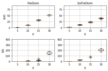
Figure 2: SHD and SID metrics for Experiment 1.

Experiment 2: Data from the non-linear SVAR Model.

Similar to [21], we simulate dataset from $X_{1}(t)=b_{11}X_{2}(t)^{2}+b_{12}X_{1}(t-1)+b_{13}X_{2}(t-1)^{2}+u_{1}(t),\,X_{2}(t)=b_{22}X_{2}(t-1)+u_{2}(t),\,X_{3}(t)=b_{31}X_{1}(t)^{3}+b_{32}X_{2}(t-1)^{2}+b_{33}X_{3}(t-1)+u_{3}(t),\,X_{4}(t)=\mbox{exp}(b_{41}X_{3t})+b_{42}X_{4}(t-1)+u_{4}(t)$ , where $u_{i}(t)\sim N(0,1)$ and $b_{ij}\sim U[-0.1,-0.4]\cup[0.1,0.4]$. Figure 3 shows the simulation results. As we can see, FreDom and ExFreDom report the best results.

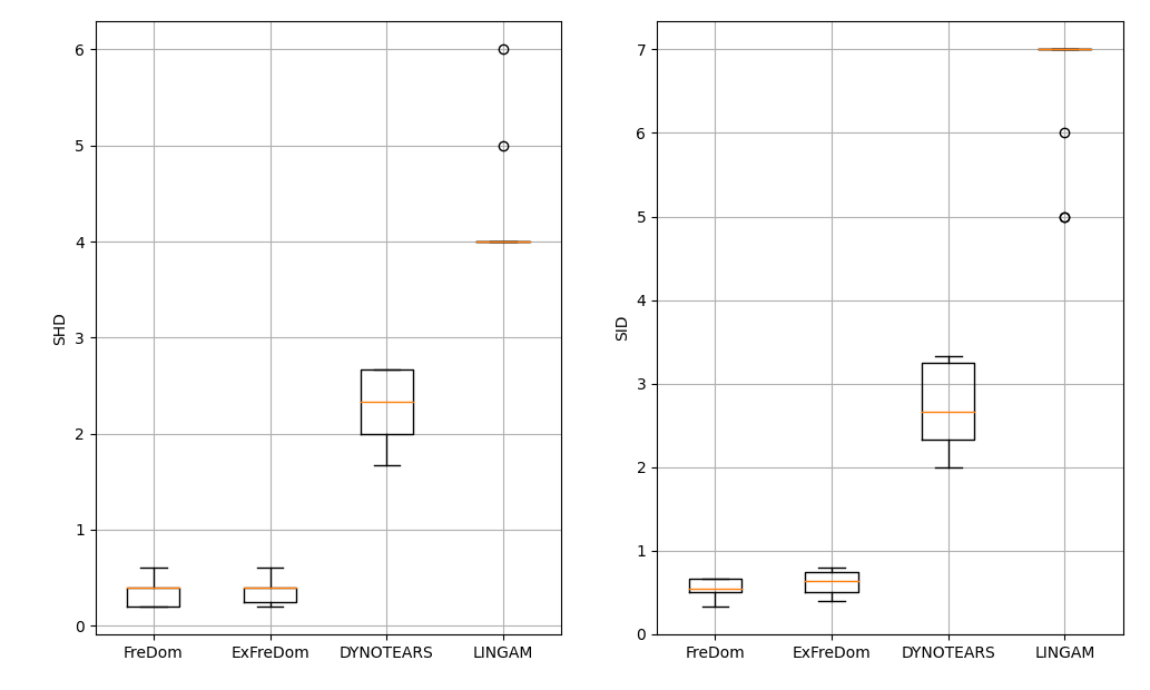
Figure 3: SHD and SID metrics for Experiment 2.

4.2 Air Pollution Data

We use (Ex)FreDom to estimate a summary DAG for 5 time series of air pollutants of length 8370. The series were recorded hourly during the year 2006 at Azusa, California. Data can be obtained from the Air Quality and Meteorological Information System. Recorded variables include CO and NO (pollutants mainly emitted from the cars and industry), $\mbox{NO}_{2}$ and $\mbox{O}_{3}$ (generated from different reactions in the atmosphere), and the global solar radiation intensity R. The similar datasets were analyzed in [64] and [65].

Figure 11 in Appendix G shows an average daily plot of five variables. Due to early morning traffic, CO and NO increase early, resulting in $\mbox{NO}_{2}$ increase. Higher $\mbox{NO}_{2}$ levels increase the Ozone ($\mbox{O}_{3}$) and the global radiation levels throughout the day.

Following [64], we apply FreDom to the residual series after subtracting the daily averages, as shown in Figure 11. The missing values in the original series are filled in by interpolating the residual series using splines. Figure 4(a) and Figure 4(b) report the estimated summary DAGs from FreDom and ExFreDom, respectively. The weights on the edges report the absolute values of the partial spectral coherence, which are frequency domain analogues of partial correlations. Additional results for LINGAM, NOTEARS, and Granger causality are available in Appendix G.

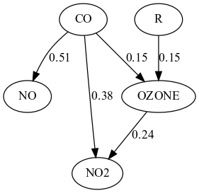
(a) FreDom

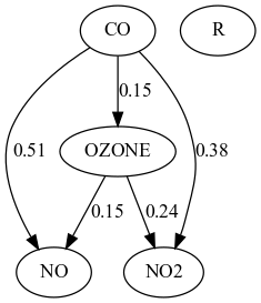
(b) ExFreDom

Figure 4: The estimated DAG from the air pollution data.

The summary DAG of FreDom correctly reflects the effect of global radiation R plays on $\mbox{O}_{3}$ generation. FreDom is also capturing the generation of $\mbox{NO}_{2}$ from $CO$ and the contemporaneous relation of CO and NO as the latter two pollutants are emitted from cars. However, we cannot validate the direction of the edge from the CO to NO. The direction of the arrow from $O_{3}$ to $\mbox{NO}_{2}$ is reversed since $\mbox{O}_{3}$ is created from $\mbox{NO}_{2}$. Compared to FreDom, ExFreDom misses edge from R to $\mbox{O}_{3}$ and has an additional edge that correctly captures the effect of CO on $\mbox{NO}_{2}$.

4.3 Stock Return Volatility Data

In this section, we analyze stock return volatility data. Data is taken from [66], where authors estimate the global bank network connectedness. Original data contains 96 banks from 29 developed and emerging economies (countries) from September 12, 2003, to February 7, 2014. For illustration purposes, we select only economies where the number of banks in each economy is greater than 4, total of 54 banks (for more details, please refer to [66]).

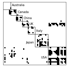
Figure 5: Estimated adjacency matrix with rows and columns sorted by country.

Figure 5 illustrates the estimated adjacency matrix from the FreDom algorithm. The rows and columns are sorted by country. As can be seen, banks from the same country tend to compose groups, meanwhile being connected to banks from the other countries. The latter result have been confirmed in many macro-economic studies [66]. The other interesting finding that needs more investigation is the causal relationship between UK and US banks. A similar result for the ExFreDom can be found in Appendix H.

5 Conclusion

In this paper, we propose a frequency domain approach to recover the topological ordering of time series. Given the ordering, we propose a penalized likelihood approach to learn the summary DAG. The proposed algorithm effectively works for both real and complex-valued data.

For future work, we left the consideration of situations in which time series suffer from unobserved confounders or undersampling, as well as theoretical results on the probability bounds for recovering a true topological ordering of the summary DAG.

Appendix A Steps For (13) Minimization

We appeal to the alternating direction method of multipliers (ADMM) [50] for minimization. The ADMM minimizes the scaled augmented Lagrangian

$$\begin{split}\mathcal{L}_{\rho}(\Theta[\cdot],Z,U[\cdot])&=\sum_{n=1}^{M}N[-\log\mbox{det}(L^{H}(n)L(n))+\mbox{tr}(\tilde{S}(n)L^{H}(n)L(n))]\\ &+{\rho}\sum_{n=1}^{M}\|L(n)-Z+U(n)\|_{F}^{2}+P(Z,\lambda),\end{split}$$ (20)

Given $(L^{(k)}[\cdot],Z^{(k)},U^{(k)}[\cdot])$ matrices in the $k$th iteration, the ADMM algorithm implements the following three updates for the next ($k+1$) iteration:

1. $L^{(k+1)}[\cdot]\leftarrow\operatorname*{arg\,min}_{L[\cdot]}\mathcal{L}_{\rho}(\Theta[\cdot],Z^{(k)},U^{(k)}[\cdot])$

2. $Z^{(k+1)}\leftarrow\operatorname*{arg\,min}_{Z}\mathcal{L}_{\rho}(L^{(k+1)}[\cdot],Z[\cdot],U^{(k)}[\cdot])$

3. $U^{(k+1)}[\cdot]\leftarrow U^{(k)}[\cdot]+(L^{(k+1)}[\cdot]-Z^{(k+1)}[\cdot])$

We use Wirtinger calculus to solve (20). For details on Wirtinger calculus, see [67, 68, 54]. It is instructive to note that for the update $L(\cdot)$, (20) can be separated into $M$ parallel problems. Thus, for $n=1,\dots,M$ we solve

$$N [-\log\mbox{det}(L^{H}(n)L(n)+\mbox{tr}(\tilde{S}(n)L^{H}(n)L(n))]$$ (21)

$$+ \rho\sum_{ij}(L_{ij}(n)-Z_{ij}-U_{ij}(n))^{*}(L_{ij}(n)-Z_{ij}-U_{ij}(n))$$

Let $\boldsymbol{\beta}^{i}=(L_{ij}(n))^{i}_{j=1}$ denote the vector of lower triangular and diagonal entries in the $i$th row of $L(n)$, and $\tilde{S}_{i}$ denote the $i\times i$ submatrix of $\tilde{S}(n)$. Then after some algebra the following identities follow:

1. $\log\mbox{det}(L^{H}(n)L(n)=2\sum_{i=1}^{p}\log\beta_{i}^{i}$

2. $\mbox{tr}(\tilde{S}(n)L^{H}(n)L(n))=\sum_{i=1}^{p}(\boldsymbol{\beta}^{i})^{H}\tilde{S}_{i}\boldsymbol{\beta}^{i}$

Using the above results, (21) can be written as a $p$ separate problems:

$$Q(\boldsymbol{\beta}^{i})=\sum_{i=1}^{p} \Big{\{}N[(\boldsymbol{\beta}^{i})^{H}\tilde{S}_{i}\boldsymbol{\beta}^{i}-2\log\beta^{i}_{i}]+$$ (22)

$$\rho \sum_{j=1}^{i-1}(\beta^{i}_{j}-Z^{i}_{j}-U^{i}_{j})^{*}(\beta^{i}_{j}-Z^{i}_{j}-U^{i}_{j})\Big{\}},$$

where $Z^{i}$ and $U^{i}$ are the vector of lower triangular and diagonal values in the $i$th row of $Z$ and $U$, respectively. We represent (22) in a generic functional form $h:C^{k-1}\times R_{+}\rightarrow R$

$$h_{k,A,\rho}=N[-2\log x_{k}+\boldsymbol{x}^{h}A\boldsymbol{x}]+\rho\sum_{j=1}^{k-1}(x_{j}-z_{j}-u_{j})^{*}(x_{j}-z_{j}-u_{j}),$$ (23)

where $Q(\boldsymbol{\beta}^{i})=h_{i,\tilde{S}_{i},\rho}(\boldsymbol{\beta}^{i})$ for $1\leq i\leq p$.

Since $h_{k,A,\rho}$ is convex, a sufficient and necessary condition for a global optimum is

$$\frac{\partial h_{k,A,\rho}}{\partial x^{*}}=0.$$

Using coordinatewise minimization algorithm and Wirtinger calculus, the following lemma follows.

Lemma A.1.

A minimizer of (23) can be computed in a closed form.

$$x_{j}=\frac{\rho(z_{j}+u_{j})-N(\sum_{l\neq j}A_{lj}x_{l})}{NA_{jj}+\rho}$$ (24)

for $1\leq j\leq k-1$, and

$$x_{k}=\frac{-\mbox{Re}(\sum_{l\neq k}A_{l}kx_{l})+\sqrt{\mbox{Re}(\sum_{l\neq k}A_{l}kx_{l})^{2}+4A_{kk}}}{2A_{kk}}$$ (25)

In Lemma A.1, for complex number $a$, $\mbox{Re}(a)$ denotes the real part.

Update (b)

From (20), the update of $Z$ is equivalent to solving complex Lasso problem. In particular, a necessary and sufficient condition for a global minimum of $Z$ is that the subdifferential of $Q(Z)={\rho}\sum_{n=1}^{M}\|L(n)-Z+U(n)\|_{F}^{2}+P(Z,\lambda)$ must contain $\boldsymbol{0}$

$$\boldsymbol{0}\in-\sum_{n=1}^{M}[L(n)-Z+U(n)]+\frac{\lambda}{\rho}\boldsymbol{\Gamma},$$ (26)

where the $ij$th component $\Gamma_{ij}=Z_{ij}/|Z_{ij}|$ if $Z_{ij}\neq 0$ and $\Gamma_{ij}\in\{u:|u|\leq 1,u\in C\}$ otherwise. Thus, $ij$th component of update (b) solution is

$$Z_{ij}=\frac{S_{\lambda/\rho}(A_{ij})}{M},$$

where $A_{ij}=\sum_{n=1}^{M}(L(n)+U(n))_{ij}$, and $S_{\lambda}(\cdot)$ is the soft-thresholding operator.

Appendix B Steps for (19) Minimization

Similar to NOTEARS, we use augmented Lagrangian method to solve the optimization problem (19), where the constrained optimization problem is reformulated as a sequence of unconstrained problems. For details, see [69]. For (19), the augmented Lagrangian is given by

$$\mathcal{L}_{\alpha,\rho_{1},\rho_{2}}(B[\cdot],Z,U[\cdot]) =\sum_{n=1}^{M}\ell(B(n);\boldsymbol{d}(n))+P(Z,\lambda)+\alpha h(Z)+\rho_{1}h(Z)^{2}+$$ (27)

$$\rho_{2}\sum_{n=1}^{M}(\|L(n)-Z+U(n)\|_{F}^{2}-\|U(n)\|_{F}^{2}),$$

Similar to (13), the ADMM algorithm implements the following four updates for the next ($k+1$) iteration:

1. $B^{(k+1)}[\cdot]\leftarrow\operatorname*{arg\,min}_{B[\cdot]}\mathcal{L}_{\rho}(\Theta[\cdot],Z^{(k)},U^{(k)}[\cdot])$

2. $Z^{(k+1)}\leftarrow\operatorname*{arg\,min}_{Z}\mathcal{L}_{\rho}(B^{(k+1)}[\cdot],Z,U^{(k)}[\cdot])$

3. $U^{(k+1)}[\cdot]\leftarrow U^{(k)}[\cdot]+(B^{(k+1)}[\cdot]-Z^{(k+1)})$

4. $\alpha^{(k+1)}\leftarrow\alpha^{(k)}+\rho_{1}^{(k)}h(Z^{(k+1)})$

The updates of (a)-(d) are similar to [52], thus we omit the derivation and only discuss the implementation details. Both NOTEARS-ADMM and NOTEARS-MLP-ADMM algorithm in [52] is implemented with PyTorch [70] and use L-BFGS method to solve the unconstrained optimization problem in the augmented Lagrangian method. Since PyTorch graciously handles Wirtinger calculus for complex-valued data, at that end, no modification needed. However, L-BFGS is designed for real-valued data. To adapt L-BFGS for the complex-valued data, we apply a well known trick [67] where before passing the matrix $Z\in C^{p\times p}$ to the optimizer, its real and imaginary parts of are concatenated into real valued $R^{2p\times p}$ matrix. The corresponding code is provided in the Supplementary Materials.

To apply ExFreDom to the $X\in R^{n\times p}$ data, first we take a Fourier transform of the data, then separate it into $M$ equal parts, where $M\in[5,10]$ and run (19) minimization.

Appendix C Proof of Lemma 3.2

Similar to [40], we define $K=(k_{ji})=(I-B)^{-1}$ such that the total effect $k_{ji}$ is the sum over all possible directed paths from $i$ to $j$ of products of complex-valued coefficient matrix $B$. From (8), $\mbox{var}(\boldsymbol{Y}_{j})=T^{-1}\sum_{l=1}^{p}k_{jl}k^{*}_{lj}$. Consequently, if $\Pi^{G}_{j}=\emptyset$ then $k_{jl}=0$ and $\mbox{var}(\boldsymbol{Y}_{j})=T^{-1}$. On the other hand, if $\Pi^{G}_{j}\neq\emptyset$ then there exist at least one parent $l\in\Pi^{G}_{j}$ whose descendants are not in the parent set, otherwise the acyclicity assumption will be violated. For $l$, $k_{jl}k^{*}_{lj}=\beta_{jl}\beta^{*}_{jl}\geq\eta$ and the result follows.

Appendix D Additional Simulation Results

In this section we compare our FreDom algorithm with two recent time series structure learning algorithms: DYNOTEARS [22] and VARLINGAM [8]. In Appendix I, to show the advantage of the frequency domain approach over the time domain, we introduce TSEqVar algorithm, which similar to extensions proposed in [8, 14, 22], is a two-step time domain extension of the [40].

The DYNOTEARS and VARLIGNAM algorithms are implemented using python packages causalenex and lingam, respectively. TSEqVar is a modification of the EqVarDAG R package [40]. It is important to note that, DYNOTEARS and VARLIGNAM are designed for analyzing only real-valued time series.

Experiment A: Small Linear SVAR Model.

In this experiment, we simulate data from the lag 1 linear SVAR $\mathbf{X}(t)=B_{0}\mathbf{X}(t)+B_{1}\mathbf{X}(t-1)+\mathbf{u}(t)$ model, where the adjacency matrices for $B_{0}$ and $B_{1}$ are

$$\begin{pmatrix}0&1&0&0&0\\ 0&0&0&0&0\\ 0&0&0&0&0\\ 0&0&1&0&0\\ 0&0&0&1&0\\ \end{pmatrix}\mbox{ and }\begin{pmatrix}0&1&1&0&0\\ 0&0&1&0&0\\ 0&0&0&0&0\\ 1&0&0&0&0\\ 0&0&0&1&0\\ \end{pmatrix}$$

Here $B_{0}$ entails the instantaneous effects, and $u_{i}(t)\sim 0.4N(0,1)$. Figure 6 reports the results. Here, FreDom performs the best.

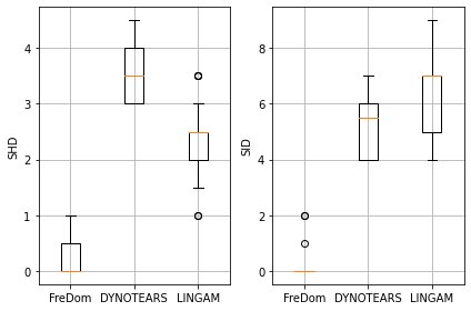
Figure 6: SHD and SID metrics for Experiment A.

Experiment B: Large linear SVAR Model.

For $K=\{15,30\}$, we generate data from the SVAR($p$) model with $p=3$ and 3 clusters (communities) of $K/3$ nodes each. Nodes within a community are not connected to any nodes in other communities. Figure 7 illustrates the non-zero patterns for the instantaneous effects and block diagonal coefficient matrices, respectively. In Appendix E, we show that for such SVAR(p) process, when the covariance matrix of error terms is identity, the inverse spectral density matrix has the same non-zero pattern as coefficient matrix (i.e., Figure 7(Right) and its Cholesky factor has the same non-zero pattern as the instantaneous effects. Consequently, from (5), the true summary DAG is known.

Figure 7: Non-zero pattern of instantaneous effect (Left) and coefficient matrix (Right) in Experiment B.

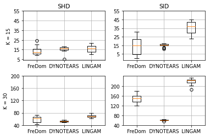
Figure 8: SHD and SID metrics for Experiment B. The rows correspond to K = {15,30}, respectively.

Figure 8 presents the results, in which rows corresponds to $K=\{15,30\}$ and columns to SHD and SID, respectively. We can see that for all $K$, FreDom reports the best SID and SHD metrics

Experiment C: Data from cSCM:

In this experiment we generate complex-valued iid data from multiple linear cSCM that share the same DAG structure. The true DAGs are simulated using the Erdos-Renyi model with the number of edges equal to number of variables $p=10$. The real and imaginary parts of the complex-valued coefficients are sampled from $[-2,-0.5]\cup[0.5,2]$ and the error term follows $N_{c}(0,1)$.

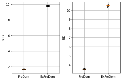
Figure 9: SHD and SID metrics for Experiment C.

Appendix E Details on Experiment B

In this section, we show that for a SVAR(p) process generated as in Experiment B in Section D and with the identity covariance matrix of error terms, the inverse spectral density matrix and its Cholesky factor have the same non-zero pattern as the coefficient matrix and instantaneous effects, respectively.

It is well known that for a VAR($p$) process with coefficient matrices $A_{1},\dots,A_{p}$, the inverse spectrum is a trigonometric matrix polynomial [71]

$$\Theta(\omega)=\mathbf{A}^{H}(e^{i\omega})\Sigma^{-1}\mathbf{A}(e^{i\omega})=X_{0}+\sum_{k=1}^{p}(e^{-ik\omega}X_{k}+e^{ik\omega}X^{T}_{k}),$$ (28)

where $X_{k}=\sum_{i=0}^{p-k}A^{T}_{i}\Theta A_{i+k}$ with $A_{0}=I$. Recalling that the relationship between VAR($p$) and SVAR($p$) coefficient matrices is $A_{i}=(I-B_{0})^{-1}B_{1}$ [8] and plugging $\Sigma$ as an identity in (28), after some algebra the result follows.

Appendix F Details on Experiment 1

The following proposition, which is a simple modification of [63, Theorem 1], states that (7) can be used to generate a complex time series whose topological order and spectrum are identical to the given order and spectrum at Fourier frequencies.

Proposition F.1.

Let $S(\omega)=(1/T)(I_{p}-B(\omega))^{-1}\{(I_{p}-B(\omega))^{-1}\}^{H}$ be a positive definite spectral density matrix and the time series is generated as in (7) then

1. $S_{T}(\omega_{k})=S(\omega_{k})$ for $\omega_{k}=k/T$, where $S_{T}(\omega)$ is the spectrum of $\mathbf{X}(t)$

2. if $S(\omega)$ has continuous second derivative with respect to $\omega$, then, for any $\omega\in[0,1]$, $|S_{T}(\omega)-S(\omega)|=O(T^{-1})$

Appendix G Air Pollution Additional Results

In this section we report an additional results for the Air Pollution dataset discussed in Section 4.2. Figure 11 reports the average of daily measurements and in Figure 10 we report the instantaneous effects obtained from the LINGAM, DYNOTEARS, and the Granger Causality Graph. The weights on the edges in Figure 10(a,b) show the corresponding estimated coefficients of instantaneous effects.

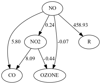
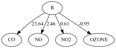
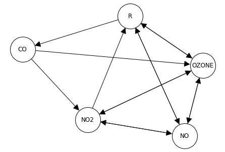
Figure 10: Additional results for the air pollution data. (a) LINGAM (b) NOTEARS (c) Granger

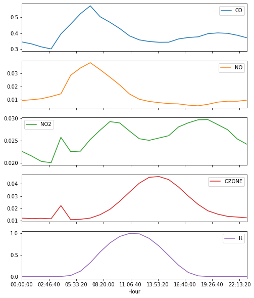
Figure 11: Average of daily measurements for the five pollutants

Appendix H Stock Return Volatility Data

Figure 12 illustrate the summary graph for the ExFreDom algorithm.

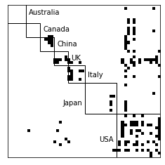
Figure 12: Estimated adjacency matrix with rows and columns sorted by country.

Appendix I TSEqVar algorithm

TSEqVar is a two-step, time domain extension of the EqVar [40]. Recall that linear SVAR with lag $p_{0}$ is given

$$\mathbf{X}(t)=B_{0}\mathbf{X}(t)+B_{1}\mathbf{X}(t-1)+\dots B_{p_{0}}\mathbf{X}(t-p_{0})+\boldsymbol{\varepsilon}(t),$$ (29)

and the relation between VAR and SVAR coefficient matrices is $B_{i}=(I-B_{0})A_{i}$. Similar to [8, 14, 22], TSEqVar implements the following two steps:

1. Run VAR($p_{0}$) model to obtain residuals and $\hat{A}_{i}$

2. Run EqVar algorithm on residuals to recover matrix $\hat{B}_{0}$ and $\hat{B}_{i}=(I-\hat{B}_{0})\hat{A}_{i}$

Table 1 report the simulation results for TSEqVar for Experiments 2 and 4.

Table 1: Mean and Standard Deviations for Experiments B and C over 50 repetitions.

	K	SHD $\tau$	SID
Exp. B	15	32.33(13.52)	28.33(16.32)
	30	135.80(35.36)	125.95(34.89)
Exp. C	4	6.05(1.22)	8.95(3.36)

References

- [1] Peters J, Janzing D, Schlkopf B. Elements of causal inference: Foundations and learning algorithms. The MIT Press; 2017.
- [2] Bessler DA, Yang J. The structure of interdependence in international stock markets. Journal of International Money and Finance. 2003;22(2):261–287.
- [3] Demiralp S, Hoover K. Searching for the causal structure of a vector autoregression. Oxford Bulletin of Economics and Statistics. 2003;65:745–767.
- [4] Runge J, Nowack P, Kretschmer M, et al. Detecting and quantifying causal associations in large nonlinear time series datasets. Science Advances. 2019;5(11).
- [5] Runge J, Bathiany S, Bollt E, et al. Inferring causation from time series in earth system sciences. Nature Communications. 2019;10.
- [6] Breitung J, Swanson NR. Temporal aggregation and spurious instantaneous causality in multiple time series models. Econometrics eJournal. 2002;.
- [7] Rajaguru G, Abeysinghe T. Temporal aggregation, cointegration and causality inference. Economics Letters. 2008;101(3):223–226.
- [8] Hyvärinen A, Zhang K, Shimizu S, et al. Estimation of a structural vector autoregression model using non-gaussianity. J Mach Learn Res. 2010;11:1709–1731.
- [9] White H, Lu X. Granger causality and dynamic structural systems. Journal of Financial Econometrics. 2010;8:193–243.
- [10] Danks D, Plis S. Learning causal structure from undersampled time series; 2013.
- [11] Gong M, Zhang K, Schoelkopf B, et al. Discovering temporal causal relations from subsampled data. In: Proceedings of the 32nd International Conference on Machine Learning; (Proceedings of Machine Learning Research; Vol. 37); 2015. p. 1898–1906.
- [12] Plis S, Danks D, Freeman C, et al. Rate-agnostic (causal) structure learning. Advances in neural information processing systems. 2015;:3303–3311.
- [13] Swanson NR, Granger CWJ. Impulse response functions based on a causal approach to residual orthogonalization in vector autoregressions. Journal of the American Statistical Association. 1997;92(437):357–367.
- [14] Moneta A, Spirtes P. Graphical models for the identification of causal structures in multivariate time series models. In: Proceedings of the 9th Joint International Conference on Information Sciences (JCIS-06). Atlantis Press; 2006. p. 613–616.
- [15] Spirtes P, Glymour C. An algorithm for fast recovery of sparse causal graphs. Social Science Computer Review. 1991;9(1):62–72.
- [16] Moneta A, Entner D, Hoyer PO, et al. Causal inference by independent component analysis: Theory and applications. Oxford Bulletin of Economics and Statistics. 2013;75(5):705–730.
- [17] Dallakyan A. Nonparanormal Structural VAR for Non-Gaussian Data. Computational Economics. 2020;0:1–21.
- [18] Entner D, Hoyer P. On causal discovery from time series data using fci; 2010.
- [19] Malinsky D, Spirtes P. Causal structure learning from multivariate time series in settings with unmeasured confounding. In: Proceedings of 2018 ACM SIGKDD Workshop on Causal Disocvery; (Proceedings of Machine Learning Research; Vol. 92); 2018. p. 23–47.
- [20] Chu T, Glymour C. Search for additive nonlinear time series causal models. Journal of Machine Learning Research. 2008;9(32):967–991.
- [21] Peters J, Janzing D, Schölkopf B. Causal inference on time series using restricted structural equation models. In: Advances in Neural Information Processing Systems; Vol. 26; 2013.
- [22] Pamfil R, Sriwattanaworachai N, Desai S, et al. Dynotears: Structure learning from time-series data. ArXiv. 2020;abs/2002.00498.
- [23] Zheng X, Aragam B, Ravikumar P, et al. Dags with no tears: Continuous optimization for structure learning. In: NeurIPS; 2018.
- [24] Ombao H, Pinto M. Spectral dependence ; 2021. Available from: https://arxiv.org/abs/2103.17240.
- [25] Shajarisales N, Janzing D, Schoelkopf B, et al. Telling cause from effect in deterministic linear dynamical systems. In: Proceedings of the 32nd International Conference on Machine Learning; (Proceedings of Machine Learning Research; Vol. 37); 2015. p. 285–294.
- [26] Besserve M, Shajarisales N, Janzing D, et al. Cause-effect inference through spectral independence in linear dynamical systems: theoretical foundations ; 2021.
- [27] Peter S, Scharf L. Statistical signal processing of complex-valued data : the theory of improper and noncircular signals. Cambridge: Cambridge University Press; 2010.
- [28] Wolter M, Yao A. Complex gated recurrent neural networks ; 2018.
- [29] Wolter M, Yao A. Fourier rnns for sequence prediction. arXiv: Machine Learning. 2018;.
- [30] Yang M, Ma MQ, Li D, et al. Complex transformer: A framework for modeling complex-valued sequence. In: ICASSP 2020 - 2020 IEEE International Conference on Acoustics, Speech and Signal Processing (ICASSP); 2020. p. 4232–4236.
- [31] Lee C, Hasegawa H, Gao S. Complex-valued neural networks: A comprehensive survey. IEEE/CAA Journal of Automatica Sinica. 2022;9(8):1406–1426.
- [32] Pearl J. Causality: Models, reasoning and inference. 2nd ed. USA: Cambridge University Press; 2009.
- [33] Heckerman D, Geiger D, Chickering DM. Learning bayesian networks: The combination of knowledge and statistical data. Mach Learn. 1995 Sep;20(3):197–243.
- [34] Chickering DM. Optimal structure identification with greedy search. J Mach Learn Res. 2002;3:507–554.
- [35] Teyssier M, Koller D. Ordering-based search: A simple and effective algorithm for learning bayesian networks. In: Proceedings of the Twenty-First Conference on Uncertainty in Artificial Intelligence; Arlington, Virginia, USA. AUAI Press; 2005. p. 584–590.
- [36] Loh PL, Bühlmann P. High-dimensional learning of linear causal networks via inverse covariance estimation. J Mach Learn Res. 2014;15(1):3065–3105.
- [37] Shimizu S, Hoyer PO, Hyvärinen A, et al. A linear non-gaussian acyclic model for causal discovery. Journal of Machine Learning Research. 2006;7(72):2003–2030.
- [38] Peters J, Mooij JM, Janzing D, et al. Causal discovery with continuous additive noise models. Journal of Machine Learning Research. 2014;15(58):2009–2053. Available from: http://jmlr.org/papers/v15/peters14a.html.
- [39] Zhang K, Wang Z, Zhang J, et al. On estimation of functional causal models: General results and application to the post-nonlinear causal model. ACM Trans Intell Syst Technol. 2015;7(2). Available from: https://doi.org/10.1145/2700476.
- [40] Chen W, Drton M, Wang YS. On causal discovery with an equal-variance assumption. Biometrika. 2019 09;106(4):973–980.
- [41] Bareinboim E, Correa J, Ibeling D, et al. On Pearl’s Hierarchy and the Foundations of Causal Inference. Causal AI Lab, Columbia University; 2020. R-60.
- [42] Bollen K. Structural equations with latent variables. New York: John Wiley and Sons; 1989.
- [43] Andersen H, Hojbjerre M, Sorensen D, et al. Linear and graphical models for the multivariate complex normal distribution. New York: Springer-Verlag; 1995.
- [44] Brockwell PJ, Davis RA. Time series: Theory and methods. New York, NY, USA: Springer-Verlag New York, Inc.; 1986.
- [45] Brillinger DR. Time series: Data analysis and theory. Philadelphia, PA, USA: Society for Industrial and Applied Mathematics; 1981.
- [46] Peters J, Bühlmann P. Identifiability of Gaussian structural equation models with equal error variances. Biometrika. 2013 11;101(1):219–228.
- [47] Ghoshal A, Honorio J. Learning linear structural equation models in polynomial time and sample complexity. In: Proceedings of the Twenty-First International Conference on Artificial Intelligence and Statistics; (Proceedings of Machine Learning Research; Vol. 84); 2018. p. 1466–1475.
- [48] Stoica P, Moses R. Introduction to spectral analysis. Prentice Hall; 1997.
- [49] Rockafellar RT. Convex analysis. Princeton University Press; 1970. Princeton Mathematical Series.
- [50] Boyd S, Parikh N, Chu E, et al. Distributed optimization and statistical learning via the alternating direction method of multipliers. Found Trends Mach Learn. 2011;3(1):1–122.
- [51] Dallakyan A, Kim R, Pourahmadi M. Time series graphical lasso and sparse var estimation. Computational Statistics & Data Analysis. 2022;176:107557.
- [52] Ng I, Zhang K. Towards federated bayesian network structure learning with continuous optimization. In: Camps-Valls G, Ruiz FJR, Valera I, editors. Proceedings of The 25th International Conference on Artificial Intelligence and Statistics; (Proceedings of Machine Learning Research; Vol. 151); 28–30 Mar. PMLR; 2022. p. 8095–8111.
- [53] Wirtinger W. Zur formalen theorie der funktionen von mehr komplexen veränderlichen. Mathematische Annalen. 1927;97:357–376.
- [54] Brandwood DH. A complex gradient operator and its application in adaptive array theory. IEE Proceedings F - Communications, Radar and Signal Processing. 1983;130(1):11–16.
- [55] Bouboulis P, Slavakis K, Theodoridis S. Adaptive learning in complex reproducing kernel hilbert spaces employing wirtinger’s subgradients. IEEE Transactions on Neural Networks and Learning Systems. 2012;23:425–438.
- [56] Ombao HC, Raz JA, Strawderman RL, et al. A simple generalised crossvalidation method of span selection for periodogram smoothing. Biometrika. 2001;88(4):1186–1192.
- [57] Dahlhaus R. Fitting time series models to nonstationary processes. Ann Statist. 1997 02;25(1):1–37.
- [58] Dallakyan A, Pourahmadi M. Fused-lasso regularized cholesky factors of large nonstationary covariance matrices of replicated time series. Journal of Computational and Graphical Statistics. 2022;0(0):1–14.
- [59] Wei W. Time series analysis univariate and multivariate methods. Pearson Education; 2006.
- [60] Zheng X, Dan C, Aragam B, et al. Learning sparse nonparametric dags. (Proceedings of Machine Learning Research; Vol. 108). PMLR; 2020. p. 3414–3425.
- [61] Peters J, Bühlmann P. Structural intervention distance for evaluating causal graphs. Neural Comput. 2015;27(3):771–799.
- [62] Foygel R, Drton M. Extended bayesian information criteria for gaussian graphical models. In: Advances in neural information processing systems 23; 2010. p. 604–612.
- [63] Dai M, Guo W. Multivariate spectral analysis using cholesky decomposition. Biometrika. 2004;91(3):629–643.
- [64] Dahlhaus R, Eichler M. Causality and graphical models in time series analysis. In: P G, N H, S R, editors. Highly structured stochastic systems. Chapter 4. Oxford: Oxford University Press; 2003.
- [65] Davis RA, Zang P, Zheng T. Sparse vector autoregressive modeling. Journal of Computational and Graphical Statistics. 2016;25(4):1077–1096.
- [66] Demirer M, Diebold FX, Liu L, et al. Estimating global bank network connectedness. Journal of Applied Econometrics. 2018;33(1):1–15.
- [67] Remmert R. Theory of complex functions. New York: Springer-Verlag; 1991.
- [68] Kreutz-Delgado K. The complex gradient operator and the cr-calculus ; 2009.
- [69] Bertsekas D. Nonlinear programming. Athena Scientific; 2016.
- [70] Paszke A, Gross S, Massa F, et al. Pytorch: An imperative style, high-performance deep learning library. Curran Associates Inc.; 2019.
- [71] Songsiri J, Dahl J, Vandenberghe L. Graphical models of autoregressive processes. Cambridge University Press; 2009. p. 89–116.