DisCo-CLIP: A Distributed Contrastive Loss
for Memory Efficient CLIP Training

Abstract

We propose DisCo-CLIP, a distributed memory-efficient CLIP training approach, to reduce the memory consumption of contrastive loss when training contrastive learning models. Our approach decomposes the contrastive loss and its gradient computation into two parts, one to calculate the intra-GPU gradients and the other to compute the inter-GPU gradients. According to our decomposition, only the intra-GPU gradients are computed on the current GPU, while the inter-GPU gradients are collected via all_reduce from other GPUs instead of being repeatedly computed on every GPU. In this way, we can reduce the GPU memory consumption of contrastive loss computation from $\mathcal{O}(B^{2})$ to $\mathcal{O}(\frac{B^{2}}{N})$, where $B$ and $N$ are the batch size and the number of GPUs used for training. Such a distributed solution is mathematically equivalent to the original non-distributed contrastive loss computation, without sacrificing any computation accuracy. It is particularly efficient for large-batch CLIP training. For instance, DisCo-CLIP can enable contrastive training of a ViT-B/32 model with a batch size of 32K or 196K using 8 or 64 A100 40GB GPUs, compared with the original CLIP solution which requires 128 A100 40GB GPUs to train a ViT-B/32 model with a batch size of 32K. The code will be released at https://github.com/IDEA-Research/DisCo-CLIP

1 Introduction

Vision-language representation learning from massive image-text pairs has recently attracted tremendous attention for its great potential in many applications such as zero-shot classification and text-image retrieval. Representative works include CLIP [27], ALIGN [17], Florence [47], CoCa [46], and BASIC [26], which all leverage hundreds of millions or even billions of image-text pairs collected from the Web to learn a semantic-rich and language-aligned visual representation [22]. As the web-collected data inevitably contain noises, CLIP [27] for the first time applies contrastive learning on 400M image-text pairs, which implies a weak but more proper assumption about the data: the relevance between paired image and text is greater than that between unpaired image and text. For its demonstrated performance in CLIP, contrastive learning has been widely adopted in subsequent works. Accordingly, several image-text data sets with increasingly larger scales have also been developed and made publicly available, such as Conceptual 12M [3], YFCC 100M [38], WIT 37.6M [37], LAION-400M [35], and LAION-5B [34].

The goal of contrastive learning in CLIP is to learn an alignment between image and text via two encoders. That is, it encourages paired image and text (called a positive pair) to be similar and meanwhile enforces unpaired image and text (called a negative pair) to be dissimilar. For any positive image-text pair, as there are normally unlimited number (up to the total number of images or texts in a data set) of negative image-text pairs, it is crucial to include a sufficiently large number of negative pairs in a contrastive loss to make the representation learning effective, as validated in all related works such as CLIP [27], Florence [47], OpenCLIP [16], and BASIC [26]. Specifically, BASIC shows that larger batch size, plus larger data set and larger model, theoretically lead to a better generalization performance.

However, a fundamental technical challenge in training a CLIP-like model is how to enlarge its batch size under the constraint of limited GPU memory. For instance, when the batch size is 65,536, the similarity matrix for all image-text pairs in the batch will cost about 16GB using Float32. As the backbone part also consumes a significant portion of GPU memory, especially for large backbones such as ViT-Large or ViT-Huge [9], scaling up batch size presents a great challenge, usually requiring hundreds of V100 or A100 GPUs [27, 47, 16], which are inaccessible for most research scientists.

In this work, we develop a distributed solution called DisCo-CLIP for constrastive loss computation, which can save a large amount of memory for contrastive loss and make CLIP training more memory-efficient. Our method starts from a decomposition of the original contrastive loss. Based on this decomposition, we divide the contrastive loss into two parts, one to calculate the intra-GPU loss and gradients, and the other one to calculate the inter-GPU loss and gradients. For a mini-batch on the $n$-th GPU (hereinafter called its hosting GPU), its intra-GPU gradients are calculated on its hosting GPU, and its inter-GPU gradients are collected from other GPUs. DisCo is an exact solution, mathematically equivalent to the original non-distributed contrastive loss, but more memory- and computation-efficient. It can decrease the memory cost of contrastive loss from $\mathcal{O}(B^{2})$ to $\mathcal{O}(\frac{B^{2}}{N})$, where $B$ and $N$ are the batch size and the number of GPUs. When $N$ equals to 64, it means around 97% (see Sec. 4.1 for details) of the memory, and similarly the computational cost, in contrastive loss can be saved. Thus, using DisCo in CLIP, we can enable contrastive training with a larger batch size. Using 8 Nvidia A100 40GB GPUs, DisCo-CLIP can enable contrastive training of a ViT-B/32 model with a batch size of 32,768. Using 64 A100 40GB GPUs, DisCo-CLIP can train the same model with a larger batch size of 196K.

We summarize our contributions in twofold.

• We propose a novel distributed contrastive loss solution called DisCo for memory efficient CLIP training, which can significantly reduce the memory consumption of the contrastive loss computation. Such a solution enables a larger batch size for contrastive training using the same computing resource without sacrificing any computation accuracy.

• We further validate that training with a larger batch size can further improve the performance of contrastive learning models.

2 Background and Related Work

In this section, we will introduce some background information for contrastive language-image pre-training (CLIP) and review some works that reduce memory consumption of the backbone part by trading computation for memory.

2.1 Contrastive Language-Image Pre-training

The idea behind CLIP [27] is to learn two representations via two encoders, an image encoder [14, 20, 9, 23, 42] and a text encoder [8, 28, 2]. Its target is to encourage positive image-text pairs to have higher similarities, and enforce negative image-text pairs to have lower similarities. The training is supervised by two contrastive losses, an image-to-text loss and a text-to-image loss. Suppose we have $B$ text-image pairs as a batch sending to two encoders and the model is trained using $N$ GPUs, with each GPU assigned $b=\frac{B}{N}$ pairs. Here, we use $\mathrm{T}_{A},\mathrm{I}_{A}$ to denote all text and image features obtained from two encoders. Suppose the hidden dimension is $D$, then the shapes of $\mathrm{T}_{A},\mathrm{I}_{A}$ are both $B\times D$. In this way, our contrastive losses can be written as,

$$\centering\mathcal{L}=\mathcal{L}_{1}(\mathrm{I}_{A},\mathrm{T}_{A})+\mathcal{L}_{2}(\mathrm{T}_{A},\mathrm{I}_{A}),\@add@centering$$ (1)

where $\mathcal{L}_{1}(\mathrm{I}_{A},\mathrm{T}_{A})$ denotes the image-to-text loss, and $\mathcal{L}_{2}(\mathrm{T}_{A},\mathrm{I}_{A})$ represents the text-to-image loss. The image-to-text loss means that the loss is to encourage a given image to find its paired text from tens of thousands of texts, and similarly for the text-to-image loss.

Motivated by the success of CLIP, many new methods have been proposed, such as FILIP [43], LiT [48], ALIGN [17], BASIC [26], BLIP [21], GIT [41], and K-LITE [36]. FILIP attempts to obtain a fine-grained alignment between image patches and text words. In contrast, CLIP only obtains an image-level alignment between an image and a text sentence. FILIP achieves this goal by a modified contrastive loss. Instead of training both image and text models from scratch, LiT [48] shows that employing a pre-trained image model and locking it would greatly benefit zero-shot classification. Under the contrastive framework, ALIGN [17] and BASIC [26] investigate how the scaling up of model, data, and batch size benefits contrastive learning. Instead of only leveraging contrastive learning framework, BLIP [21] introduces a mixed contrastive learning and generative learning for vision-language model. Further, GIT [41] employs a pure generative learning framework and demonstrates its superior performance.

The success of CLIP and the above methods highly depends on large-scale paired image-text data set [3, 38, 37, 17, 35, 34]. Compared with classification data sets, such as ImageNet 1K [7] and ImageNet 21K [33], which require careful human annotation, there are abundant paired image-text data on the Web and can be more easily collected [34].

Large batch size is a prerequisite for vision-language contrastive learning. Data Parallelism (DP) and Model Parallelism (MP) are two widely used methods in deep learning for distributed training [44, 45, 39, 8, 12, 28]. There are many related works on this topic, such as DeepSpeed [29, 30, 31] and Colossal-AI [1]. We recommend interested readers to refer to these papers for some common distributed learning techniques. In the following, we will describe several methods that trade computation for memory in the backbone part.

2.2 Trade Computation for Memory in Backbone

Checkpointing [5] is an effective approach to reduce memory consumption, especially for the intermediate results of low-cost operation. It only stores feature maps of some high-cost operations, such as convolution, MLP, and self-attention, but drops feature maps of low-cost operations such as activation (e.g., ReLU, GeLU) and layer normalization in the forward pass. In the backward process, these dropped feature maps can be recomputed quickly at a low cost. By dropping some intermediate feature maps, we can save a great amount of memory. Gruslys et al. [13] further extend the idea of Checkpointing to the recursive neural network. Checkpointing is helpful but still not sufficient if we want to further increase the batch size.

Recently, BASIC [26] introduces a gradient accumulating (GradAccum) method for memory saving in backbone via micro-batching the contrastive loss. This approach is based on the observation that when computing the contrastive loss, we only need the full similarity matrix instead of all intermediate results. Thus, BASIC proposes to trade computation for memory by dropping some intermediate hidden states during the forward process, and then re-compute them during back-propagation. This method can effectively reduce the memory consumption in the backbone part but it requires one extra forward computation. A similar gradient cache approach [10] was also introduced for dense passage retriever in natural language processing.

Reversible model structure [11, 19] is another elegant method for memory saving in backbone. However, it requires block adaption because it needs to reconstruct the input layer according to the output layer in the back propagation process. Reversible structure is particularly suitable for models that do not change activation shape in the whole network. However, reconstructing a layer from its output inevitably takes more backward time.

All above three mechanisms mainly focus on reducing memory consumption in the backbone part. However, none of them pays attention to reducing the memory consumption of the contrastive loss, which has been a big bottleneck for large batch size contrastive training. We will explain this problem in the next section.

Figure 1: Illustration of the original CLIP training. All image features $\mathrm{I}_{A}$ and text features $\mathrm{T}_{A}$ are gathered to every GPU via all_gather to calculate the $B\times B$ similarity matrix for contrastive loss computation. This computation is performed repeatedly on every GPU.

3 Motivation

Distributed contrastive learning is different from traditional distributed data parallel and model parallel strategies. Data parallel (DP) is particularly effective when activations in the network cost most of the GPU memory. For example, in [12], Goyal et al. succeeded in training an ImageNet classification model in one hour. Each GPU independently performs forward and backward computation. Only after backward computation, the GPUs perform a gradient communication to merge gradients. In contrast, model parallel (MP) is more effective when model parameters (e.g. 10 billions of parameters) consume a large mount of GPU memory. In this way, the model parameters are sliced and assigned to different GPUs. However, different from the DP and MP problems, in contrastive training, besides the backbone and model parameters, the contrastive loss consumes a larger amount of GPU memory especially when a large batch size is used.

As we have discussed in the introduction section, a large batch size is of crucial importance for contrastive learning. Previous research [26] also proves theoretically that a larger contrastive batch size can lead to a better representation for image-text models. Interested readers can refer to Theorem 1 in [26] and its appendix for the proof.

However, a large batch in contrastive loss will consume a large amount of GPU memory, usually of $\mathcal{O}(B^{2})$, where $B$ is the batch size. Let us take an examination of the memory consumption of contrastive loss. For example, for a batch size of 65,536, it stores a similarity matrix of 4.3 billions parameters which requires 16GB of memory using Float32. Its gradient computation in the back-propagation process will take another 16GB of memory. Considering other memory cost of model parameters and backbone intermediate activations, it cannot be trained using A100 40GB GPUs even with mixed precision computation.

After investigating the constrastive loss in depth, we notice that there is much redundant memory consumption and computational waste in the current CLIP training solution. As shown in Fig. 1, in the original CLIP training, to calculate the gradients for the text and image features in the hosting GPU, every GPU in the distributed training environment needs to compute the entire $B\times B$ similarity matrix, which is not necessary as we will show later.

Our motivation in this paper is to eliminate memory redundancy and remove unnecessary calculation via a loss decomposition, and thus enable large batch training using limited GPU resource.

4 DisCo-CLIP: A Distributed Contrastive Loss for Memory Efficient CLIP Training

In this section, we introduce DisCo, a distributed solution for contrastive loss computation. Using DisCo in CLIP, we accomplish a new memory efficient CLIP training method, called DisCo-CLIP. To this end, we decompose the loss calculation into two parts, one part to compute the intra-GPU loss and gradients and the other part to compute inter-GPU loss and gradients. This section will first introduce how we decompose this loss calculation. Then, we will describe the algorithm implementation of DisCo-CLIP in detail.

4.1 DisCo: A Distributed Contrastive Loss

As shown in Eq. 1, $\mathrm{I}_{A}$ and $\mathrm{T}_{A}$ denote all image and text features collected from all GPUs. Here, we use $\mathrm{I}_{n}$ and $\mathrm{T}_{n}$ to denote the image and text features on the $n$-th GPU, and use $\mathrm{I}_{\overline{n}}$ and $\mathrm{T}_{\overline{n}}$ to denote the image and text features on all other GPUs. The division is denoted as,

$$\mathrm{I}_{A} =[\mathrm{I}_{n},\ \ \mathrm{I}_{\overline{n}}],$$ (2)

$$\mathrm{T}_{A} =[\mathrm{T}_{n},\ \mathrm{T}_{\overline{n}}]$$

The shapes of $\mathrm{I}_{A}$ and $\mathrm{T}_{A}$ are $B\times D$, the shapes of $\mathrm{I}_{n}$ and $\mathrm{T}_{n}$ are $\frac{B}{N}\times D$, and the shapes of $\mathrm{I}_{\overline{n}}$ and $\mathrm{T}_{\overline{n}}$ are $\frac{B(N-1)}{N}\times D$.

According to the above definition, the contrastive loss can be decomposed and rewritten as,

$$\mathcal{L}_{d}=\mathcal{L}_{1}(\mathrm{I}_{n},\mathrm{T}_{A})+\mathcal{L}_{1}(\mathrm{I}_{\overline{n}},\mathrm{T}_{A})+$$ (3)

$$\mathcal{L}_{2}(\mathrm{T}_{n},\mathrm{I}_{A})+\mathcal{L}_{2}(\mathrm{T}_{\overline{n}},\mathrm{I}_{A}),$$

where $\mathcal{L}_{1}(\mathrm{I}_{n},\mathrm{T}_{A})$ denotes the image-to-text contrastive loss between image features $\mathrm{I}_{n}$ and text features $\mathrm{T}_{A}$, and $\mathcal{L}_{2}(\mathrm{T}_{n},\mathrm{I}_{A})$ denotes the text-to-image loss between $\mathrm{T}_{n}$ and $\mathrm{I}_{A}$. Mathematically, the computational result $\mathcal{L}_{d}$ in Eq. 3 is the same as the result $\mathcal{L}$ in Eq. 1. However, by decomposing the loss $\mathcal{L}_{d}$ into four parts, the gradient flow in the back-propagation process is more obvious. Meanwhile, we can see that $\mathcal{L}_{1}(\mathrm{I}_{\overline{n}},\mathrm{T}_{A})$ does not induce gradients with respect to $\mathrm{I}_{n}$ and $\mathcal{L}_{2}(\mathrm{T}_{\overline{n}},\mathrm{I}_{A})$ has no gradients with respect to $\mathrm{T}_{n}$. Actually, these two terms are redundant computation on the $n$-th GPU in the original contrastive loss, which unnecessarily consume a large amount of memory.

Thus, according to the decomposition in Eq. 3, we can calculate the gradients $\frac{\partial\mathcal{L}_{d}}{\partial\mathrm{I}_{n}}$ for image features $\mathrm{I}_{n}$, and the gradients $\frac{\partial\mathcal{L}_{d}}{\partial\mathrm{T}_{n}}$ for text features $\mathrm{T}_{n}$ as follows,

$$\frac{\partial\mathcal{L}_{d}}{\partial\mathrm{I}_{n}} =\mathchoice{\leavevmode\hbox to214.35pt{\vbox to14.52pt{\text{[drawing]}}}}{\leavevmode\hbox to214.35pt{\vbox to14.52pt{\text{[drawing]}}}}{\leavevmode\hbox to150.04pt{\vbox to10.16pt{\text{[drawing]}}}}{\leavevmode\hbox to107.17pt{\vbox to7.26pt{\text{[drawing]}}}}+\mathchoice{\leavevmode\hbox to104.77pt{\vbox to14.79pt{\text{[drawing]}}}}{\leavevmode\hbox to104.77pt{\vbox to14.79pt{\text{[drawing]}}}}{\leavevmode\hbox to78.14pt{\vbox to11.04pt{\text{[drawing]}}}}{\leavevmode\hbox to60.38pt{\vbox to8.53pt{\text{[drawing]}}}}, \mathstrut\frac{\partial\mathcal{L}_{1}(\mathrm{I}_{n},\mathrm{T}_{A})}{\partial\mathrm{I}_{n}}+\frac{\partial\mathcal{L}_{2}(\mathrm{T}_{n},\mathrm{I}_{A})}{\partial\mathrm{I}_{n}} \mathstrut\frac{\partial\mathcal{L}_{2}(\mathrm{T}_{\overline{n}},\mathrm{I}_{A})}{\partial\mathrm{I}_{n}} \mathstrut\frac{\partial\mathcal{L}_{1}(\mathrm{I}_{n},\mathrm{T}_{A})}{\partial\mathrm{I}_{n}}+\frac{\partial\mathcal{L}_{2}(\mathrm{T}_{n},\mathrm{I}_{A})}{\partial\mathrm{I}_{n}} \mathstrut\frac{\partial\mathcal{L}_{2}(\mathrm{T}_{\overline{n}},\mathrm{I}_{A})}{\partial\mathrm{I}_{n}}$$ (4)

$$\frac{\partial\mathcal{L}_{d}}{\partial\mathrm{T}_{n}} =\mathchoice{\leavevmode\hbox to214.35pt{\vbox to14.52pt{\text{[drawing]}}}}{\leavevmode\hbox to214.35pt{\vbox to14.52pt{\text{[drawing]}}}}{\leavevmode\hbox to150.04pt{\vbox to10.16pt{\text{[drawing]}}}}{\leavevmode\hbox to107.17pt{\vbox to7.26pt{\text{[drawing]}}}}+\mathchoice{\leavevmode\hbox to104.77pt{\vbox to14.79pt{\text{[drawing]}}}}{\leavevmode\hbox to104.77pt{\vbox to14.79pt{\text{[drawing]}}}}{\leavevmode\hbox to78.14pt{\vbox to11.04pt{\text{[drawing]}}}}{\leavevmode\hbox to60.38pt{\vbox to8.53pt{\text{[drawing]}}}}, \mathstrut\frac{\partial\mathcal{L}_{1}(\mathrm{I}_{n},\mathrm{T}_{A})}{\partial\mathrm{T}_{n}}+\frac{\partial\mathcal{L}_{2}(\mathrm{T}_{n},\mathrm{I}_{A})}{\partial\mathrm{T}_{n}} \mathstrut\frac{\partial\mathcal{L}_{1}(\mathrm{I}_{\overline{n}},\mathrm{T}_{A})}{\partial\mathrm{T}_{n}} \mathstrut\frac{\partial\mathcal{L}_{1}(\mathrm{I}_{n},\mathrm{T}_{A})}{\partial\mathrm{T}_{n}}+\frac{\partial\mathcal{L}_{2}(\mathrm{T}_{n},\mathrm{I}_{A})}{\partial\mathrm{T}_{n}} \mathstrut\frac{\partial\mathcal{L}_{1}(\mathrm{I}_{\overline{n}},\mathrm{T}_{A})}{\partial\mathrm{T}_{n}}$$

where the losses in the red part can be further unfolded in a sum form as,

$$\frac{\partial\mathcal{L}_{2}(\mathrm{T}_{\overline{n}},\mathrm{I}_{A})}{\partial\mathrm{I}_{n}} =\sum_{i\neq n\And i\in[1,N]}\frac{\partial\mathcal{L}_{2}(\mathrm{T}_{i},\mathrm{I}_{A})}{\partial\mathrm{I}_{n}},$$ (5)

$$\frac{\partial\mathcal{L}_{1}(\mathrm{I}_{\overline{n}},\mathrm{T}_{A})}{\partial\mathrm{T}_{n}} =\sum_{j\neq n\And j\in[1,N]}\frac{\partial\mathcal{L}_{1}(\mathrm{I}_{j},\mathrm{T}_{A})}{\partial\mathrm{T}_{n}}.$$

The gradients of $\frac{\partial\mathcal{L}_{d}}{\partial\mathrm{I}_{n}}$ and $\frac{\partial\mathcal{L}_{d}}{\partial\mathrm{T}_{n}}$ both consist of three terms. In both equations, all three terms can be divided into two parts, we mark them with two different colors, blue and red. The gradients in the blue part are calculated on the $n$-th (hosting) GPU, and the gradients in the red part are calculated on other GPUs. We call them intra-GPU gradients and inter-GPU gradients, respectively. When computing the red part for $\frac{\partial\mathcal{L}_{d}}{\partial\mathrm{I}_{n}}$, the images $\mathrm{I}_{n}$ are considered as negative samples. It should be noted that although $\mathrm{I}_{n}$ is regarded as negative samples, there still induce gradients for $\mathrm{I}_{n}$.

Figure 2: Illustration of the gradient calculation of DisCo on the first GPU. In DisCo, to calculate the gradients on the current GPU, we only need to compute two $\frac{B}{N}\times B$ similarity matrices instead of a full $B\times B$ matrix as shown in Fig. 1.

According to this decomposition, to compute $\frac{\partial\mathcal{L}_{d}}{\partial\mathrm{I}_{n}}$ and $\frac{\partial\mathcal{L}_{d}}{\partial\mathrm{T}_{n}}$, the $n$-th GPU only needs to compute the following four terms,

$$\footnotesize\mathchoice{\leavevmode\hbox to424.43pt{\vbox to14.52pt{\text{[drawing]}}}}{\leavevmode\hbox to424.43pt{\vbox to14.52pt{\text{[drawing]}}}}{\leavevmode\hbox to297.1pt{\vbox to10.16pt{\text{[drawing]}}}}{\leavevmode\hbox to212.21pt{\vbox to7.26pt{\text{[drawing]}}}}. \mathstrut\left[\frac{\partial\mathcal{L}_{1}(\mathrm{I}_{n},\mathrm{T}_{A})}{\partial\mathrm{I}_{n}},\frac{\partial\mathcal{L}_{2}(\mathrm{T}_{n},\mathrm{I}_{A})}{\partial\mathrm{I}_{n}},\frac{\partial\mathcal{L}_{1}(\mathrm{I}_{n},\mathrm{T}_{A})}{\partial\mathrm{T}_{n}},\frac{\partial\mathcal{L}_{2}(\mathrm{T}_{n},\mathrm{I}_{A})}{\partial\mathrm{T}_{n}}\right] \mathstrut\left[\frac{\partial\mathcal{L}_{1}(\mathrm{I}_{n},\mathrm{T}_{A})}{\partial\mathrm{I}_{n}},\frac{\partial\mathcal{L}_{2}(\mathrm{T}_{n},\mathrm{I}_{A})}{\partial\mathrm{I}_{n}},\frac{\partial\mathcal{L}_{1}(\mathrm{I}_{n},\mathrm{T}_{A})}{\partial\mathrm{T}_{n}},\frac{\partial\mathcal{L}_{2}(\mathrm{T}_{n},\mathrm{I}_{A})}{\partial\mathrm{T}_{n}}\right]$$ (6)

All four terms only need to compute two small similarity matrices of shape $\frac{B}{N}\times B$ instead of a full matrix of shape $B\times B$ which consumes a large amount of memory. In this way, we can reduce memory consumption from $B^{2}$ to $\frac{2B^{2}}{N}$. For instance, when $N=16$, we save $\frac{7}{8}$ of memory consumption, if $N$ is 64, we save $\frac{31}{32}$ of memory consumption. Meanwhile, it also saves much computation. The computational cost for the contrastive similarity matrix decreases from $B^{2}D$ to $\frac{2B^{2}D}{N}$.

For the two red terms in Eq. 4,

$$\footnotesize\mathchoice{\leavevmode\hbox to230.87pt{\vbox to14.79pt{\text{[drawing]}}}}{\leavevmode\hbox to230.87pt{\vbox to14.79pt{\text{[drawing]}}}}{\leavevmode\hbox to171.21pt{\vbox to11.04pt{\text{[drawing]}}}}{\leavevmode\hbox to131.43pt{\vbox to8.53pt{\text{[drawing]}}}}, \mathstrut\left[\frac{\partial\mathcal{L}_{2}(\mathrm{T}_{\overline{n}},\mathrm{I}_{A})}{\partial\mathrm{I}_{n}},\frac{\partial\mathcal{L}_{1}(\mathrm{I}_{\overline{n}},\mathrm{T}_{A})}{\partial\mathrm{T}_{n}}\right] \mathstrut\left[\frac{\partial\mathcal{L}_{2}(\mathrm{T}_{\overline{n}},\mathrm{I}_{A})}{\partial\mathrm{I}_{n}},\frac{\partial\mathcal{L}_{1}(\mathrm{I}_{\overline{n}},\mathrm{T}_{A})}{\partial\mathrm{T}_{n}}\right]$$ (7)

we use the all_reduce operation to perform gradient communication and collect all gradients with respect to $\mathrm{I}_{n}$ and $\mathrm{T}_{n}$. Fig. 2 illustrates the gradient calculation of DisCo on the first of $N$ GPUs.

Let us compare DisCo with the original contrastive loss. In the original implementation, because of the lack of gradient communication in the process of back-propagation among GPUs, each GPU must compute the whole similarity matrix between $\mathrm{I}_{A}$ and $\mathrm{T}_{A}$ to obtain the gradients $\frac{\partial\mathcal{L}_{d}}{\partial\mathrm{I}_{n}}$ and $\frac{\partial\mathcal{L}_{d}}{\partial\mathrm{T}_{n}}$ on the $n$-th GPU. In DisCo, for each GPU, we only need to calculate a subset instead of the whole similarity matrix. We then use an all_reduce operation to conduct gradient communication and collect the gradients. The distributed contrastive loss can also be applied to the contrastive loss computation in self-supervised learning [6, 4].

4.2 Algorithm Implementation of DisCo-CLIP

# image_encoder: ResNet or ViT

# text_encoder: text Transformer

# img[b,H,W,C]: minibatch of images

# text[b,L]: minibatch of texts

# t: temperature parameter

# D: feature dimension

# N: nums of GPU

# rank: global rank

 

# extract feature representations

i_e = image_encoder(img) # [b,D]

t_e = text_encoder(text) # [b,D]

 

# gather features from all gpus

I_E = all_gather(i_e) # [N,b,D]

T_E = all_gather(t_e) # [N,b,D]

 

# scaled dot product similarities

logits_i = dot(I_E[rank], T_E)*t # [b,N*b]

logits_t = dot(T_E[rank], I_E)*t # [b,N*b]

 

# image-to-text and text-to-image losses

labels = arange(b) + b * rank

loss_i = cross_entropy_loss(logits_i, label)

loss_t = cross_entropy_loss(logits_t, label)

 

# loss backward

loss = (loss_i + loss_t) / 2

loss.backward()

 

# reduce gradients and losses from all gpus

I_E.grad = all_reduce(I_E.grad, op=AVG)

T_E.grad = all_reduce(T_E.grad, op=AVG)

Loss = all_reduce(loss, op=AVG)

 

# backbone backward

i_e.backward(I_E.grad[rank])

t_e.backward(T_E.grad[rank])

Algorithm 1 Pseudo-code for DisCo-CLIP

Using DisCo in CLIP, we develop a memory efficient CLIP training method, termed as DisCo-CLIP. To make our algorithm clearer, we show the pseudo-code for DisCo-CLIP in Alg. 1. The implementation can be roughly divided into three segments. In the first segment, for each GPU with a global rank number, we extract its image and text features, and then use all_gather to collect image and text features into this GPU. Then in the second segment, we compute the similarity matrix and the two losses: image-to-text and text-to-image, and use the losses to compute the gradients. In this segment, the intra-GPU gradients, $\left[\frac{\partial\mathcal{L}_{1}(\mathrm{I}_{n},\mathrm{T}_{A})}{\partial\mathrm{I}_{n}},\frac{\partial\mathcal{L}_{2}(\mathrm{T}_{n},\mathrm{I}_{A})}{\partial\mathrm{I}_{n}},\frac{\partial\mathcal{L}_{1}(\mathrm{I}_{n},\mathrm{T}_{A})}{\partial\mathrm{T}_{n}},\frac{\partial\mathcal{L}_{2}(\mathrm{T}_{n},\mathrm{I}_{A})}{\partial\mathrm{T}_{n}}\right]$, as defined in Eq. 6, will be computed on the current GPU. In the last segment, we use all_reduce to finish gradient communication. In this segment, the inter-GPU gradients, $\left[\frac{\partial\mathcal{L}_{2}(\mathrm{T}_{\overline{n}},\mathrm{I}_{A})}{\partial\mathrm{I}_{n}},\frac{\partial\mathcal{L}_{1}(\mathrm{I}_{\overline{n}},\mathrm{T}_{A})}{\partial\mathrm{T}_{n}}\right]$, as defined in Eq. 7, will be collected to the current GPU. The intra-GPU and inter-GPU gradients are averaged to obtain $\left[\frac{\partial\mathcal{L}_{d}}{\partial\mathrm{I}_{n}},\frac{\partial\mathcal{L}_{d}}{\partial\mathrm{T}_{n}}\right]$. Finally, we perform backward propagation for the backbone.

DisCo-CLIP has two advantages compared with CLIP. First, it decreases the memory consumption for the contrastive loss from $\mathcal{O}(B^{2})$ to $\mathcal{O}(\frac{B^{2}}{N})$. Second, it reduces the computational complexity of the contrastive loss from $\mathcal{O}(B^{2}D)$ to $\mathcal{O}(\frac{B^{2}}{N}D)$. Besides these two advantages, DisCo-CLIP is an exact solution for CLIP without sacrificing any computation accuracy.

Note that DisCo-CLIP requires an extra all_reduce operator to perform gradient communication, which has the same cost as the all_gather operator. Compared with the full similarity matrix computation, this extra communication cost is quite small and negligible. See Table 4 for a speed comparison.

For the backbone part, we can also use the GradAccum strategy as proposed in BASIC [26]. BASIC provides a simple yet effective memory-efficient strategy for backbone memory optimization. Combined with GradAccum, DisCo-CLIP can further lead to a more memory-efficient solution.

Methods	Backbone	Contra. Loss	Overall
CLIP[27]	$\mathcal{O}\left(\frac{B}{N}LD\right)$	$\mathcal{O}\left(B^{2}\right)$	$\mathcal{O}(\frac{B}{N}LD)$ + $\mathcal{O}(B^{2})$
BASIC[26]	$\mathcal{O}\left(\frac{B}{N}D\right)$	$\mathcal{O}\left(B^{2}\right)$	$\mathcal{O}(\frac{B}{N}D)$+$\mathcal{O}(B^{2})$
DisCo-CLIP	$\mathcal{O}\left(\frac{B}{N}LD\right)$	$\mathcal{O}\left(\frac{B^{2}}{N}\right)$	$\mathcal{O}(\frac{B}{N}LD)$ + $\mathcal{O}(\frac{B^{2}}{N})$
$\text{DisCo-CLIP}^{*}$	$\mathcal{O}\left(\frac{B}{N}D\right)$	$\mathcal{O}\left(\frac{B^{2}}{N}\right)$	$\mathcal{O}(\frac{B}{N}D)$ + $\mathcal{O}(\frac{B^{2}}{N})$

Table 1: Memory consumption comparison of different methods. $\text{DisCo-CLIP}^{*}$ denotes the combination of DisCo-CLIP and the GradAccum strategy in BASIC. $B$ denotes the batch size, which is usually very large, e.g. 32K, $N$ is the number of GPUs, $L$ is the number of layers in the backbone, and $D$ is the feature dimension. For simplicity, we use the same $D$ for all layers.

A detailed comparison of memory consumption for CLIP, BASIC, and DisCo-CLIP is provided in Table 1. With GradAccum, BASIC can reduce the overall memory consumption from $\mathcal{O}(\frac{B}{N}LD)+\mathcal{O}(B^{2})$ to $\mathcal{O}(\frac{B}{N}D)+\mathcal{O}(B^{2})$. DisCo-CLIP can reduce the memory consumption to $\mathcal{O}(\frac{B}{N}LD)+\mathcal{O}(\frac{B^{2}}{N})$, $\text{DisCo-CLIP}^{*}$ can further reduce the memory consumption to $\mathcal{O}(\frac{B}{N}D)+\mathcal{O}(\frac{B^{2}}{N})$. A practical example is that, in vanilla CLIP [27] based on ViT-B/32, $D=1024,B=32768,N=128$.

5 Experiments

In this section, we first describe the experimental settings including data sets and pre-training details. Then, we present the experiments regarding memory consumption, training efficiency, batch size, and data scale. Finally, we report zero-shot classification on several data sets.

5.1 Experimental Setting

Image-Text Data Sets. A large-scale image-text data set is a prerequisite for contrastive image-text pre-training. In the literature, there are many private [37, 17] or public data sets [38, 35, 34]. LAION-400M [35] is a data set with 400 million image-text pairs filtered by CLIP score. We crawl the images according to the provided URLs and finally obtain 360M image-text pairs as some URLs are expired and no longer available. LAION-5B [34] is a larger data set with 5 billion image-text pairs. It contains a subset of 2.32 billion English image-text pairs. We refer to this subset as LAION-2B as in [34]. We also crawl the data set according to the released URLs and finally obtain 2.1 billion image-text pairs. In this paper, for a fair comparison with CLIP [27] and LAION [34] which conduct experiments using 400M data pairs, we create a subset of 400M image-text pairs from our crawled LAION-2B and also make a subset of 100M image-text pairs for ablation study.

Pre-training Details. The implementation of our DisCo-CLIP is based on OpenCLIP [16], an open source CLIP implementation. We follow the original CLIP [27] and mainly use ViT-B/32 [9] as the vision backbone.Training images are resized to $224\times 224$ and fed to the vision backbone. For the text backbone, we use a text Transformer [39, 8], and set the maximum length of text to 76 as in  [27]. Due to limited time and GPU resource, we do not train ViT-L/14 because it takes more than four times of training time compared to ViT-B/32. It should also be noted that in all our experiments, we do not use the GradAccum strategy as in BASIC [26]. Checkpointing is enabled in vanilla CLIP and our DisCo-CLIP. We train models using an Adam [18] optimizer and cosine learning rate scheduler with a linear warmup [24]. Weight decay regularization [25] is used on all parameters except bias, layer normalization, and temperature in contrastive loss. Since our training experiments use different batch sizes, according to previous works [12, 28], we change the learning rate for different batch sizes. For our learning rate scheduler, we first define a base learning rate of 5e-4 and a base batch size of 32,768, and then linearly warm it up to the maximum learning rate. The maximum learning rate is determined according to a linear strategy, $\text{max\_lr = base\_lr}*\frac{\text{batch size}}{\text{32,768}}$. Training stability is a challenging issue in mixed-precision training as NaN might happen in many cases. We obverse that $\beta_{2}$ in Adam is very important for training stability and find 0.98 works well for our experiments instead of the default value of 0.999. For most of our experiments, we use 64 NVIDIA A100 40GB GPUs for model training, but for some experiments, we only use 8 NVIDIA A100 40GB GPUs to show that our solution is more resource-efficient.

5.2 Evaluation Results

Equivalence Validation. To empirically validate our theoretical analysis, we conduct experiments to compare CLIP and DisCo-CLIP. We use the same random seed to initiate the network parameters and use the same batch size 32,768 on 64 GPUs, and train ViT-B/32 models with 16 epochs on LAION-100M.

Methods	Memory	Accuracy	Time (Hours)
CLIP	27.4GB	51.64	13.4
DisCo-CLIP	16.5GB	51.64	12.1

Table 2: CLIP Reproduction. Under the same training settings, DisCo-CLIP has exactly the same accuracy (top-1 zero-shot classification accuracy on ImageNet) as CLIP, but uses lower memory consumption and less training time. Training resource: 64 A100 40GB GPUs.

From Table 2, we see that DisCo-CLIP has exactly the same accuracy as CLIP, but uses lower memory consumption and less training time. Under the same training settings, DisCo-CLIP and CLIP also have exactly the same training curves. This experiment further validates the numerical equivalence between DisCo-CLIP and CLIP.

Methods	GPUs	BS	Memory
CLIP	64$\times$ A100 40GB	32,768	27.4GB
CLIP	64$\times$ A100 40GB	65,536	OOM
DisCo-CLIP	64$\times$ A100 40GB	32,768	16.5GB
DisCo-CLIP	64$\times$ A100 40GB	196,608	38.1GB
DisCo-CLIP	8$\times$ A100 40GB	32,768	36.9GB

Table 3: Memory consumption of CLIP and DisCo-CLIP under different settings. “OOM” means out of memory.

Methods	GPUs	Batch size	Backbone	Loss Operators			Loss Total	Backward		Total
				all_gather	Loss	all_reduce		Loss BP	Backbone BP
CLIP	64	32,768	129.4	6.1	55.4	-	61.5	414.8		605.6
DisCo-CLIP	64	32,768		6.1	1.6	4.3	12.0 $(80.5\%\downarrow)$	2.8	337.3	481.5 $(20.5\%\downarrow)$

Table 4: Detailed comparisons of training efficiency of CLIP and DisCo-CLIP. All time-related measurements (the last nine columns) are in millisecond (ms). DisCo-CLIP saves more computational time in loss computation. Training resource: 64 A100 40GB GPUs.

Memory Consumption. Besides memory consumption of network parameters, backbone and contrastive loss consumes most memory. We evaluate the memory consumption of the original CLIP and our DisCo-CLIP under different settings. We report the peak memory consumption for different settings, and the results are shown in Table 3.

We have three observations from Table 3. 1) CLIP with ViT-B/32 can be trained with batch size 32,768 but fails with batch size 65,536. 2) Our DisCo-CLIP can enable training of ViT-B/32 with a much larger batch size, 196,608 with 64 A100 40GB GPU. 3) DisCo-CLIP can enable training of the same model on a cluster with only 8 GPUs.

Training Speed. One iteration of CLIP consists of extracting features from backbone, gathering features from all GPUs, calculating loss, and executing back-propagation. (We exclude some other factors, including data loading and optimizer update that are not directly related to the model computation or can be ignored.) Instead, DisCo-CLIP decomposes the back-propagation into two BP processes (Loss BP and Backbone BP) and have an additional all_reduce operator. We evaluate the running time of each operator in CLIP and our DisCo-CLIP, and the results are shown in Table 4.

From Table 4, we can see that 1) for total loss computation, under the same batch size 32,768, we decrease the computation time from 61.5 ms to 12.0 ms. It is because in DisCo-CLIP, we only need to calculate two subset similarity matrices between multiplying a $\frac{B}{N}\times D$ matrix and a $B\times D$ matrix instead of a full matrix multiplication between two $B\times D$ matrices. 2) the operators of both all_reduce and all_gather are faster compared to the loss computation. 3) under the same batch size 32,768, DisCo-CLIP improves around $20.5\%$ total training efficiency.

Overall, with DisCo-CLIP, we are able to not only train contrastive learning models with a larger batch size, but also improve the training speed considerably. DisCo-CLIP is a free-lunch solution for large-scale contrastive learning.

Batch Size	Steps	Epochs	ViT-B/32
8,192	$\approx 200\mathrm{~{}K}$	16	$48.76$
16,384	$\approx 100\mathrm{~{}K}$	16	$50.95$
32,768	$\approx 50\mathrm{~{}K}$	16	$51.64$
65,536	$\approx 25\mathrm{~{}K}$	16	$\mathbf{51.91}$

Table 5: Evaluation of different batch sizes on DisCo-CLIP. All models are trained for 16 epochs on a LAION-100M data set, we show top-1 zero-shot classification accuracy on ImageNet. Training resource: 64 A100 40GB GPUs.

Batch Size. To assess the role of a larger batch size to the final performance, we conduct some controlled experiments for ViT-B/32 on our LAION-100M and LAION-400M subsets. All training hyper-parameters are the same except that we vary the batch size and the number of training steps. To ensure all models “see” the same number of training samples, we use fewer training steps when training with a larger batch size. In Table 5, we report the results of all settings.

From Table 5, we can see that large batch size generally helps contrastive learning. The performance of using batch size 65,536 improves that of using batch size 32,768 by around 0.3%. In the evaluation of data scaling, we further observe that the improvement widens when we train the model for more epochs.

Batch Size	100M$\times$16	400M$\times$4	400M$\times$8
16,384	$50.95$	$54.36$	$58.38$
32,768	$51.64$	$55.52$	$59.69$
65,536	$51.91$	$55.50$	$\mathbf{59.96}$

Table 6: Evaluation of data scaling on DisCo-CLIP. Three batch sizes are evaluated with two LAION subsets: LAION-100M and LAION-400M. The numbers $\times 16$, $\times 4$, and $\times 8$ are the training epochs for each data set. Training resource: 64 A100 40GB GPUs.

Model	Data Sets	Epochs	Steps	Batch Size	INet [7]	INet-v2 [32]	INet-R [15]	INet-S [40]
CLIP [27]	CLIP WIT 400M	32	$\approx{400}\mathrm{~{}K}$	32,768	$63.3$	$56.0$	69.4	$42.3$
OpenCLIP [16, 34]	LAION-400M	32	$\approx{400}\mathrm{~{}K}$	32,768	$62.9$	$55.1$	73.4	$49.4$
DisCo-CLIP	LAION-400M∗	32	$\approx{400}\mathrm{~{}K}$	32,768	$63.2$	$55.2$	73.4	$50.6$
DisCo-CLIP	LAION-400M∗	32	$\approx{\textbf{200}}\mathrm{~{}K}$	65,536	64.3	56.2	73.8	51.7

Table 7: Comparison of DisCo-CLIP with vanilla CLIP and re-implemented CLIP by LAION group. We report top-1 zero-shot classification accuracy (%) on several data sets. All models are based on ViT-B/32. Our LAION-400M^∗ is a 400M subset of LAION-2B. Training resource: 64 A100 40GB GPUs.

Data Scaling. To investigate the role of data scaling, we also conduct some controlled experiments for ViT-B/32 on the LAION 100M and LAION 400M subsets. For all models, we use three different batch sizes, 16,384, 32,768 and 65,536 for training. Models are trained with three different settings, 100M with 16 epochs, 400M with 4 epochs and 400M with 8 epochs. Table 6 reports the final ImageNet top-1 zero-shot classification accuracy of all models.

From Table 6, we observe that, “seeing” the same number of training samples (LAION-100M with 16 epochs, LAION-400M with 4 epochs.), the model trained on larger scale of data set can obtain better performance. For example, trained with the same batch size 65,536, the performance improves from 51.91% to 55.50% when the data set increases from 100M to 400M. This observation validates the value of data scaling. This observation is also consistent with the combined scaling law in BASIC [26]. We also find that training with more epochs on larger scale of data with larger batch size will bring in larger performance gain. The gap between models (with batch sizes 32,768 and 65,536) trained on 400M with 4 epochs is around 0% (from 55.52% to 55.50%), but it increases to 0.3% (from 59.69% to 59.96%) when the models are trained for 8 epochs. Thus, we can expect that if we use larger scale of data set, we should also use larger batch size to get a better performance.

5.3 Zero-Shot Classification

Following CLIP [27] and LAION-5B [34], we evaluate zero-shot top-1 classification accuracy of our models on several data sets, including INet [7], INet-v2 [32], INet-R [15] and INet-S [40]. We use exactly the same 80 prompts as CLIP. Some standard prompts are like “a bad photo of a {}.”, “a photo of many {}.”, and etc. Following LAION-5B, we extract the embedding for each prompt using the text encoder (text Transformer), and average embeddings of all prompts in each class, and finally get the final class embedding. Given an image, we extract its image embedding via the image encoder (ViT-B/32), and compute its similarities with all class embeddings, and classify it into the class with the highest similarity score.

We can see from Table 7, that using the same batch size of 32,768 as the OpenCLIP implementation, our DisCo-CLIP obtains a similar performance with OpenCLIP, the result of OpenCLIP is reported by LAION group in [34]. Using a larger batch size of 65,536, DisCo-CLIP achieves a better performance than the OpenCLIP implementation and the original CLIP. Specifically, trained with the same 32 epochs, DisCo-CLIP using a batch size of 65,536 improves the OpenCLIP’s result that is based on batch size of 32,768 by 1.4%. Note that when doubling the batch size, we halve the training steps. This observation further validates that large batch size is important for contrastive learning.

6 Discussion

Recent developments in large-scale contrastive or generative learning, such as CLIP [27], ALIGN [17], FILIP [43], LiT [48], BASIC [26], LAION-5B [34], and GIT [41] have potential for many real-world applications, such as image classification, text-to-image retrieval, recommendation system, and generation models. Besides large-scale data sets, the progress highly depends on powerful GPU or TPU computing resources. As shown in Table 8, all methods use a large amount of computing hardwares. FILIP uses less GPU but also uses smaller batch size.

Methods	Hardware
CLIP [27]	256 NVIDIA V100 GPUs
FILIP [43]	128 NVIDIA V100 GPUs
LAION-5B [34]	128-400 NVIDIA A100 GPUs
LiT [48]	128-400 TPUs
BASIC [26]	2,048 TPUs v3

Table 8: Several vision-language contrastive learning methods and their used hardwares.

Unfortunately, only a few big technology companies can afford this task. Large batch contrastive loss consumes a large amount of GPU memory, while large batch size is a prerequisite for contrastive learning. As a result, it is challenging for companies with limited resources or academic research institutes to contribute to research on this topic. Our work provides a simple yet effective solution for reducing memory consumption that can help bridge the gap between academia and industry on this topic.

7 Conclusion

In this paper, we have proposed a simple yet effective distributed contrastive loss solution called DisCo to reduce the memory consumption in contrastive learning. By decomposing the loss computation into intra-GPU computation and inter-GPU computation, we can remove redundant memory consumption and use a all_reduce operator to collect inter-GPU gradients. Using DisCo in CLIP, the introduced DisCo-CLIP can enable a much larger batch contrastive learning compared to CLIP using the same GPU resource. Specifically, we can train DisCo-CLIP models with batch size 32,768 using 8 A100 40GB GPUs, or with batch size 196K using 64 GPUs. We hope DisCo-CLIP will also help and motivate self-supervised learning [4, 6] which also uses contrastive learning.

8 Acknowledgement

This work was partially supported by OPPO Research Fund.

9 Appendix

9.1 Training Curves

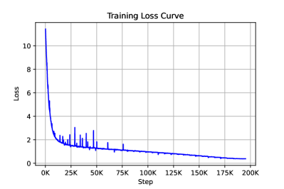
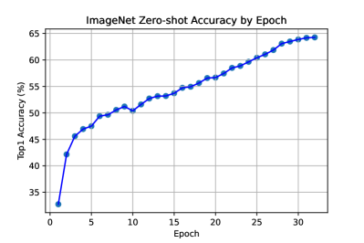
Figure 3: Curve of the training loss on the left and curve of the zero-shot top-1 ImageNet classification accuracy (%) on the right. The base model is ViT-B/32, the used batch size is 65,536. The model is trained 32 epochs on LAION-400M.

To facilitate the readers to observe the training process, we show the curves of the training loss and the zero-shot top-1 ImageNet classification in Fig. 3. The base model is ViT-B/32, the used batch size is 65,536. The model is trained 32 epochs on LAION-400M.

9.2 Zero-shot Classification Details

We follow CLIP [27] for the zero-shot classification. We use the same 80 prompts as in CLIP. During evaluation, We first resize the image to the short side 224 according to the image ratio and then centrally crop a $224\times 224$ image.

Dataset	Classes	Number of Test Images
INet [7]	1,000	50,000
INet-v2 [32]	1,000	10,000
INet-R [15]	1,000	30,000
INet-S [40]	1,000	50,889

Table 9: Information of the evaluation data sets used in our paper.

Our used evaluation datasets include INet [7], INet-v2 [32], INet-R [15] and INet-S [40]. We show some basic information in Tab. 9. More information can be found in Timm.

9.3 More Experiments

We further evaluate the performance of DisCo-CLIP under different batch sizes. The experiments are conducted on LAION-100M subset, the models are based on ViT-B/32, and the number of training epochs is 16. The results are shown in Tab. 10. We can see that from Tab. 10 larger batch size always brings in performance gain. Using DisCo-CLIP, it takes around 2 days to finish training of 16 epochs of LAION-100M with batch size 32,768 on a cluster with only 8 A100 GPUs.

Model	Datasets	Epochs	Steps	Batch Size	INet [7]	INet-V2 [32]	INet-R [15]	INet-S [40]
DisCo-CLIP	LAION-100M∗	16	${200}\mathrm{~{}K}$	8,192	${48.76}$	${41.28}$	56.67	${36.65}$
DisCo-CLIP	LAION-100M∗	16	${100}\mathrm{~{}K}$	16,384	${50.95}$	${43.07}$	59.24	${38.74}$
DisCo-CLIP	LAION-100M∗	16	${50}\mathrm{~{}K}$	32,768	${51.64}$	${43.85}$	60.07	${39.25}$
DisCo-CLIP	LAION-100M∗	16	${25}\mathrm{~{}K}$	65,536	51.91	44.19	60.52	39.76

Table 10: Performance evaluation of DisCo-CLIP under different batch size. We report top-1 zero-shot classification accuracy (%) on several data sets. All models are based on ViT-B/32. Our LAION-100M^∗ is a 100M subset of LAION-2B.

References

• [1] Zhengda Bian, Hongxin Liu, Boxiang Wang, Haichen Huang, Yongbin Li, Chuanrui Wang, Fan Cui, and Yang You. Colossal-ai: A unified deep learning system for large-scale parallel training. arXiv preprint arXiv:2110.14883, 2021.
• [2] Tom Brown, Benjamin Mann, Nick Ryder, Melanie Subbiah, Jared D Kaplan, Prafulla Dhariwal, Arvind Neelakantan, Pranav Shyam, Girish Sastry, Amanda Askell, et al. Language models are few-shot learners. Advances in Neural Information Processing Systems, 33:1877–1901, 2020.
• [3] Soravit Changpinyo, Piyush Sharma, Nan Ding, and Radu Soricut. Conceptual 12M: Pushing web-scale image-text pre-training to recognize long-tail visual concepts. In Proceedings of the IEEE/CVF Conference on Computer Vision and Pattern Recognition, pages 3558–3568, 2021.
• [4] Ting Chen, Simon Kornblith, Mohammad Norouzi, and Geoffrey Hinton. A simple framework for contrastive learning of visual representations. In International Conference on Machine Learning, pages 1597–1607. PMLR, 2020.
• [5] Tianqi Chen, Bing Xu, Chiyuan Zhang, and Carlos Guestrin. Training deep nets with sublinear memory cost. arXiv preprint arXiv:1604.06174, 2016.
• [6] Xinlei Chen, Saining Xie, and Kaiming He. An empirical study of training self-supervised vision transformers. In Proceedings of the IEEE/CVF International Conference on Computer Vision, pages 9640–9649, 2021.
• [7] Jia Deng, Wei Dong, Richard Socher, Li-Jia Li, Kai Li, and Li Fei-Fei. Imagenet: A large-scale hierarchical image database. In 2009 IEEE Conference on Computer Vision and Pattern Recognition, pages 248–255. IEEE, 2009.
• [8] Jacob Devlin, Ming-Wei Chang, Kenton Lee, and Kristina Toutanova. Bert: Pre-training of deep bidirectional transformers for language understanding. arXiv preprint arXiv:1810.04805, 2018.
• [9] Alexey Dosovitskiy, Lucas Beyer, Alexander Kolesnikov, Dirk Weissenborn, Xiaohua Zhai, Thomas Unterthiner, Mostafa Dehghani, Matthias Minderer, Georg Heigold, Sylvain Gelly, et al. An image is worth 16x16 words: Transformers for image recognition at scale. arXiv preprint arXiv:2010.11929, 2020.
• [10] Luyu Gao, Yunyi Zhang, Jiawei Han, and Jamie Callan. Scaling deep contrastive learning batch size under memory limited setup. In Proceedings of the 6th Workshop on Representation Learning for NLP (RepL4NLP-2021), pages 316–321, 2021.
• [11] Aidan N Gomez, Mengye Ren, Raquel Urtasun, and Roger B Grosse. The reversible residual network: Backpropagation without storing activations. Advances in Neural Information Processing Systems, 30, 2017.
• [12] Priya Goyal, Piotr Dollár, Ross Girshick, Pieter Noordhuis, Lukasz Wesolowski, Aapo Kyrola, Andrew Tulloch, Yangqing Jia, and Kaiming He. Accurate, large minibatch sgd: Training imagenet in 1 hour. arXiv preprint arXiv:1706.02677, 2017.
• [13] Audrunas Gruslys, Rémi Munos, Ivo Danihelka, Marc Lanctot, and Alex Graves. Memory-efficient backpropagation through time. Advances in Neural Information Processing Systems, 29, 2016.
• [14] Kaiming He, Xiangyu Zhang, Shaoqing Ren, and Jian Sun. Deep residual learning for image recognition. In Proceedings of the IEEE Conference on Computer Vision and Pattern Recognition, pages 770–778, 2016.
• [15] Dan Hendrycks, Steven Basart, Norman Mu, Saurav Kadavath, Frank Wang, Evan Dorundo, Rahul Desai, Tyler Zhu, Samyak Parajuli, Mike Guo, et al. The many faces of robustness: A critical analysis of out-of-distribution generalization. In Proceedings of the IEEE/CVF International Conference on Computer Vision, pages 8340–8349, 2021.
• [16] Gabriel Ilharco, Mitchell Wortsman, Ross Wightman, Cade Gordon, Nicholas Carlini, Rohan Taori, Achal Dave, Vaishaal Shankar, Hongseok Namkoong, John Miller, Hannaneh Hajishirzi, Ali Farhadi, and Ludwig Schmidt. Openclip, July 2021.
• [17] Chao Jia, Yinfei Yang, Ye Xia, Yi-Ting Chen, Zarana Parekh, Hieu Pham, Quoc Le, Yun-Hsuan Sung, Zhen Li, and Tom Duerig. Scaling up visual and vision-language representation learning with noisy text supervision. In International Conference on Machine Learning, pages 4904–4916. PMLR, 2021.
• [18] Diederik P Kingma and Jimmy Ba. Adam: A method for stochastic optimization. arXiv preprint arXiv:1412.6980, 2014.
• [19] Nikita Kitaev, Lukasz Kaiser, and Anselm Levskaya. Reformer: The efficient transformer. In International Conference on Learning Representations, 2019.
• [20] Alexander Kolesnikov, Lucas Beyer, Xiaohua Zhai, Joan Puigcerver, Jessica Yung, Sylvain Gelly, and Neil Houlsby. Big transfer (bit): General visual representation learning. In European Conference on Computer Vision, pages 491–507. Springer, 2020.
• [21] Junnan Li, Dongxu Li, Caiming Xiong, and Steven Hoi. Blip: Bootstrapping language-image pre-training for unified vision-language understanding and generation. arXiv preprint arXiv:2201.12086, 2022.
• [22] Liunian Harold Li, Pengchuan Zhang, Haotian Zhang, Jianwei Yang, Chunyuan Li, Yiwu Zhong, Lijuan Wang, Lu Yuan, Lei Zhang, Jenq-Neng Hwang, et al. Grounded language-image pre-training. In Proceedings of the IEEE/CVF Conference on Computer Vision and Pattern Recognition, pages 10965–10975, 2022.
• [23] Ze Liu, Yutong Lin, Yue Cao, Han Hu, Yixuan Wei, Zheng Zhang, Stephen Lin, and Baining Guo. Swin transformer: Hierarchical vision transformer using shifted windows. In Proceedings of the IEEE/CVF International Conference on Computer Vision, pages 10012–10022, 2021.
• [24] Ilya Loshchilov and Frank Hutter. Sgdr: Stochastic gradient descent with warm restarts. arXiv preprint arXiv:1608.03983, 2016.
• [25] Ilya Loshchilov and Frank Hutter. Decoupled weight decay regularization. In International Conference on Learning Representations, 2018.
• [26] Hieu Pham, Zihang Dai, Golnaz Ghiasi, Kenji Kawaguchi, Hanxiao Liu, Adams Wei Yu, Jiahui Yu, Yi-Ting Chen, Minh-Thang Luong, Yonghui Wu, et al. Combined scaling for open-vocabulary image classification. arXiv preprint arXiv: 2111.10050, 2021.
• [27] Alec Radford, Jong Wook Kim, Chris Hallacy, Aditya Ramesh, Gabriel Goh, Sandhini Agarwal, Girish Sastry, Amanda Askell, Pamela Mishkin, Jack Clark, et al. Learning transferable visual models from natural language supervision. In International Conference on Machine Learning, pages 8748–8763. PMLR, 2021.
• [28] Colin Raffel, Noam Shazeer, Adam Roberts, Katherine Lee, Sharan Narang, Michael Matena, Yanqi Zhou, Wei Li, Peter J Liu, et al. Exploring the limits of transfer learning with a unified text-to-text transformer. J. Mach. Learn. Res., 21(140):1–67, 2020.
• [29] Samyam Rajbhandari, Jeff Rasley, Olatunji Ruwase, and Yuxiong He. Zero: Memory optimizations toward training trillion parameter models. In SC20: International Conference for High Performance Computing, Networking, Storage and Analysis, pages 1–16. IEEE, 2020.
• [30] Samyam Rajbhandari, Olatunji Ruwase, Jeff Rasley, Shaden Smith, and Yuxiong He. Zero-infinity: Breaking the gpu memory wall for extreme scale deep learning. In Proceedings of the International Conference for High Performance Computing, Networking, Storage and Analysis, pages 1–14, 2021.
• [31] Jeff Rasley, Samyam Rajbhandari, Olatunji Ruwase, and Yuxiong He. Deepspeed: System optimizations enable training deep learning models with over 100 billion parameters. In Proceedings of the 26th ACM SIGKDD International Conference on Knowledge Discovery & Data Mining, pages 3505–3506, 2020.
• [32] Benjamin Recht, Rebecca Roelofs, Ludwig Schmidt, and Vaishaal Shankar. Do imagenet classifiers generalize to imagenet? In International Conference on Machine Learning, pages 5389–5400. PMLR, 2019.
• [33] Tal Ridnik, Emanuel Ben-Baruch, Asaf Noy, and Lihi Zelnik-Manor. Imagenet-21k pretraining for the masses. arXiv preprint arXiv:2104.10972, 2021.
• [34] Christoph Schuhmann, Romain Beaumont, Cade W Gordon, Ross Wightman, Theo Coombes, Aarush Katta, Clayton Mullis, Patrick Schramowski, Srivatsa R Kundurthy, Katherine Crowson, et al. Laion-5b: An open large-scale dataset for training next generation image-text models. In Thirty-sixth Conference on Neural Information Processing Systems Datasets and Benchmarks Track, 2022.
• [35] Christoph Schuhmann, Richard Vencu, Romain Beaumont, Robert Kaczmarczyk, Clayton Mullis, Aarush Katta, Theo Coombes, Jenia Jitsev, and Aran Komatsuzaki. Laion-400m: Open dataset of clip-filtered 400 million image-text pairs. arXiv preprint arXiv:2111.02114, 2021.
• [36] Sheng Shen, Chunyuan Li, Xiaowei Hu, Yujia Xie, Jianwei Yang, Pengchuan Zhang, Anna Rohrbach, Zhe Gan, Lijuan Wang, Lu Yuan, Ce Liu, Kurt Keutzer, Trevor Darrell, Anna Rohrbach, , and Jianfeng Gao. K-lite: Learning transferable visual models with external knowledge. arXiv preprint arXiv:2204.09222, 2022.
• [37] Krishna Srinivasan, Karthik Raman, Jiecao Chen, Michael Bendersky, and Marc Najork. Wit: Wikipedia-based image text dataset for multimodal multilingual machine learning. In Proceedings of the 44th International ACM SIGIR Conference on Research and Development in Information Retrieval, pages 2443–2449, 2021.
• [38] Bart Thomee, David A Shamma, Gerald Friedland, Benjamin Elizalde, Karl Ni, Douglas Poland, Damian Borth, and Li-Jia Li. Yfcc100m: The new data in multimedia research. Communications of the ACM, 59(2):64–73, 2016.
• [39] Ashish Vaswani, Noam Shazeer, Niki Parmar, Jakob Uszkoreit, Llion Jones, Aidan N Gomez, Łukasz Kaiser, and Illia Polosukhin. Attention is all you need. Advances in Neural Information Processing Systems, 30, 2017.
• [40] Haohan Wang, Songwei Ge, Zachary Lipton, and Eric P Xing. Learning robust global representations by penalizing local predictive power. Advances in Neural Information Processing Systems, 32, 2019.
• [41] Jianfeng Wang, Zhengyuan Yang, Xiaowei Hu, Linjie Li, Kevin Lin, Zhe Gan, Zicheng Liu, Ce Liu, and Lijuan Wang. Git: A generative image-to-text transformer for vision and language. arXiv preprint arXiv:2205.14100, 2022.
• [42] Haiping Wu, Bin Xiao, Noel Codella, Mengchen Liu, Xiyang Dai, Lu Yuan, and Lei Zhang. Cvt: Introducing convolutions to vision transformers. In Proceedings of the IEEE/CVF International Conference on Computer Vision, pages 22–31, 2021.
• [43] Lewei Yao, Runhui Huang, Lu Hou, Guansong Lu, Minzhe Niu, Hang Xu, Xiaodan Liang, Zhenguo Li, Xin Jiang, and Chunjing Xu. Filip: Fine-grained interactive language-image pre-training. arXiv preprint arXiv:2111.07783, 2021.
• [44] Yang You, Igor Gitman, and Boris Ginsburg. Scaling sgd batch size to 32k for imagenet training. arXiv preprint arXiv:1708.03888, 6(12):6, 2017.
• [45] Yang You, Jing Li, Sashank Reddi, Jonathan Hseu, Sanjiv Kumar, Srinadh Bhojanapalli, Xiaodan Song, James Demmel, Kurt Keutzer, and Cho-Jui Hsieh. Large batch optimization for deep learning: Training bert in 76 minutes. arXiv preprint arXiv:1904.00962, 2019.
• [46] Jiahui Yu, Zirui Wang, Vijay Vasudevan, Legg Yeung, Mojtaba Seyedhosseini, and Yonghui Wu. Coca: Contrastive captioners are image-text foundation models. arXiv preprint arXiv:2205.01917, 2022.
• [47] Lu Yuan, Dongdong Chen, Yi-Ling Chen, Noel Codella, Xiyang Dai, Jianfeng Gao, Houdong Hu, Xuedong Huang, Boxin Li, Chunyuan Li, et al. Florence: A new foundation model for computer vision. arXiv preprint arXiv:2111.11432, 2021.
• [48] Xiaohua Zhai, Xiao Wang, Basil Mustafa, Andreas Steiner, Daniel Keysers, Alexander Kolesnikov, and Lucas Beyer. Lit: Zero-shot transfer with locked-image text tuning. In Proceedings of the IEEE/CVF Conference on Computer Vision and Pattern Recognition, pages 18123–18133, 2022.