A stationary axisymmetric vacuum solution for pure $R^{2}$ gravity

Abstract

The closed-form expression for pure $\mathcal{R}^{2}$ vacuum solution obtained in Phys. Rev. D 107, 104008 (2023) lends itself to a generalization to axisymmetric setup via the modified Newman–Janis algorithm. We adopt the procedure put forth in Phys. Rev. D 90, 064041 (2014) bypassing the complexification of the radial coordinate. The procedure presumes the existence of Boyer-Lindquist coordinates. Using the Event Horizon Telescope Collaboration results, we model the central black hole M87* by the thus obtained exact rotating metric, depending on the mass, rotation parameter and a third dimensionless parameter. The latter is constrained upon investigating the shadow angular size assuming mass and rotation parameters are those of M87*. Stability is investigated.

I Introduction

The family of $f(\mathcal{R})$ theories is an active arena of research in modified gravity. It is considerably less involved than theories containing the Ricci or Riemann tensors in their action Nojiri-2011 ; Clifton-2011 ; deFelice-2010 ; Sotiriou-2008 . It is also advantaged by being ghost-free, as its scalar degree of freedom, when moving from the Jordan frame to the Einstein frame, involves derivatives no higher than two. This theory offers a number of exact analytical solutions, some of which project non-constant scalar curvature Sebastiani-2010 ; Capozziello-2007 ; Gurses-2012 ; Pravda-2017 . However, these solutions do not align with the Schwarzschild metric and fail to pass tests in the Solar System and binary stars.

Prior to proposing $f(R)$ gravity Buchdahl-1970 , Buchdahl considered the pure $R^{2}$ action around 1962, which is a simple and natural extension of General Relativity Buchdahl-1962 . Its action contains one single term in the gravitation sector, $\frac{1}{2\kappa}\int d^{4}x\sqrt{-g}\,\mathcal{R}^{2}$, making it more parsimonious than Brans-Dicke gravity which involves the Brans-Dicke parameter $\omega$, and conformal gravity which involves the nuanced Bach tensor. The action is scale invariant, with the parameter $\kappa$ being dimensionless. In vacuum, the action leads to the field equation

$$\mathcal{R}\left(\mathcal{R}_{\mu\nu}-\frac{1}{4}g_{\mu\nu}\mathcal{R}\right)+\left(g_{\mu\nu}\square-\nabla_{\mu}\nabla_{\nu}\right)\mathcal{R}=0,$$ (1)

and, consequently, the trace equation

$$\square\,\mathcal{R}=0.$$ (2)

In Buchdahl-1962 Buchdahl demonstrated that the trace equation (2) allows for a non-constant Ricci scalar field. To establish this, he expressed the metric in the “harmonic gauge” as

$$ds^{2}=-A(u)dt^{2}+B(u)du^{2}+\sqrt{B(u)/A(u)}d\Omega^{2},$$ (3)

where $A(u)$ and $B(u)$ are two unknown functions of $u$, a harmonic coordinate in the radial direction. For this metric, the d’Alembertian acting on a scalar field is

$$\square\,\mathcal{R} \equiv\frac{1}{\sqrt{-g}}\partial_{\mu}\left(\sqrt{-g}g^{\mu\nu}\partial_{\nu}\mathcal{R}\right)=B^{-1}\frac{d^{2}\mathcal{R}}{du^{2}}.$$ (4)

The trace equation in vacuum (2) directly yields $\frac{d^{2}\mathcal{R}}{du^{2}}=0$, resulting in $\mathcal{R}$ being an affine function of $u$, viz.

$$\mathcal{R}=\Lambda+k\,u,$$ (5)

where $\Lambda$ and $k$ are two constants.

Recently, one of us revisited Buchdahl’s 1962 work and discovered a class of spacetime solutions for pure $\mathcal{R}^{2}$ gravity Nguyen-2022-Buchdahl . Consistent with the finding expressed in Eq. (5), these Buchdahl-inspired solutions are asymptotically de Sitter and exhibit non-constant scalar curvature. In addition to the asymptotic value of the scalar curvature at spatial infinity, the solutions are specified by a new (Buchdahl) parameter, $k$, which has dimensions of length and is of higher-derivative nature.

The role of the Buchdahl parameter $k$ can be likened to the “scalar charge” in scalar-tensor theories. As demonstrated in Bronnikov-1998 , for the BD action $L_{\text{BD}}=\sqrt{-g}\Bigl{[}\phi\,\mathcal{R}+\frac{\omega}{\phi}\phi_{;\mu}\phi^{;\mu}\Bigr{]}$, by switching from the Jordan frame to the Einstein frame via the transformations:

$$\tilde{g}_{\mu\nu}:=\phi\,g_{\mu\nu}\ \ \ \text{and}\ \ \ \varphi:=\sqrt{|\omega+3/2|}\,\ln\phi\,,$$ (6)

the action takes the form of General Relativity with a minimally coupled scalar field $\varphi$, per

$$L_{\text{BD}}=\sqrt{-\tilde{g}}\Bigl{[}\tilde{\mathcal{R}}+\varepsilon\,\tilde{g}^{\mu\nu}\partial_{\mu}\varphi\partial_{\nu}\varphi\Bigr{]};\ \ \varepsilon:=\text{sgn}\Bigl{(}\omega+\frac{3}{2}\Bigr{)}.$$ (7)

The resulting field equations are

$$\tilde{\mathcal{R}}_{\text{\textmu}\nu} =-\varepsilon\,\partial_{\mu}\varphi\partial_{\nu}\varphi\,,$$ (8)

and

$$\tilde{\square}\,\varphi=0.$$ (9)

Similarly to the steps taken in Eqs. (3)–(5), in the harmonic coordinate $u$, the harmonic equation (9) directly yields

$$\varphi=\varphi_{0}+C\,u\,;\ \ \ \ \ \ \varphi_{0},\,C=\text{const}\,,$$ (10)

with $C$ representing a scalar charge, a notion first advanced by Bronnikov in 1973 Bronnikov-1973 . When $C=0$, the Schwarzschild metric is recovered. In general, $C\in\mathbb{R}$. The scalar charge plays a central role in generating new physics for Brans-Dicke gravity Bronnikov-1998 . For $C\neq 0$, as $\varphi$ varies, resulting in $\tilde{\mathcal{R}}_{\mu\nu}\neq 0$ in vacuum per Eq. (8), non-Schwarzschild solutions are obtained. Furthermore, it has been determined that these solutions in scalar-tensor theories are typically stable Bronnikov-1998 ; Matsuda-1972 ; Campanelli-1993 .

Considering the close analogy of the two harmonic equations, Eq. (5) vs Eq. (10), and of the pure $\mathcal{R}^{2}$ and Brans-Dicke theories , it follows that the Buchdahl parameter $k$ can be considered as the scalar charge and should take on any value in $\mathbb{R}$ unrestricted.

Within the class of Buchdahl-inspired solutions mentioned above, a specific case has been derived in Ref. Ref. Nguyen-2022-Lambda0 which provides an exact closed analytical solution describing asymptotically flat spacetimes. This special Buchdahl-inspired metric recovers Schwarzschild when the Buchdahl parameter $k$ vanishes. Yet, for $k\neq 0$, this solution exhibits novel intriguing properties for $\mathcal{R}^{2}$ spacetimes Nguyen-2022-Lambda0 . Pure $\mathcal{R}^{2}$ gravity is thus an example of a higher-order theory capable of producing a diverse range of phenomena, even in the absence of complex ingredients such as torsion, non-metricity, or non-locality.

The new metrics invite extensions to the stationary axisymmetric setup, via the use of the Newman-Janis algorithm (NJA). The method starts with a “seed” static spherically symmetric metric in a closed form

$$ds_{\text{seed}}^{2}=-G(r)dt^{2}+\frac{dr^{2}}{F(r)}+H(r)\left(d\theta^{2}+\sin^{2}\theta d\varphi^{2}\right).$$ (11)

A crucial step in the NJA is the complexification of the radial coordinate, viz. $r\rightarrow r+ia\cos\theta$, in which the following replacements are adopted:

$$r^{2} \rightarrow(r+ia\cos\theta)(r-ia\cos\theta)=r^{2}+a^{2}\cos^{2}\theta,$$ (12)

$$\frac{1}{r} \rightarrow\frac{1}{2}\left(\frac{1}{r+ia\cos\theta}+\frac{1}{r-ia\cos\theta}\right)=\frac{r}{r^{2}+a^{2}\cos^{2}\theta}.$$

For the “seed” Reissner–Nordström metric, viz. $F(r)=G(r)=1-\frac{2M}{r}+\frac{Q^{2}}{r^{2}}$ and $H(r)=r^{2}$, the NJA aptly produces the Kerr-Newman metric that describes a charged rotating black hole in General Relativity.

As the complexification scheme adopted in Eq. (12) is rather ad hoc, in Refs.  Azreg-Ainou-B ; Azreg-Ainou-C ; Azreg-Ainou-2014 , the other author of us proposed another route with a higher degree of plausibility. It assumes the existence of Boyer-Lindquist coordinates and imposes an integrability condition in some of its coordinate transformations. The procedure is an improvement over the NJA and bypasses the complexification step.

The purpose of our current paper is to apply the non-complexification technique put forth in Ref.  Azreg-Ainou-2014 to the Buchdahl-inspired solutions, in order to obtain rotating solutions for uncharged rotating sources in pure $\mathcal{R}^{2}$ gravity. We will be able to derive an exact rotating solution up to a conformal factor, the determination of which requires solving some challenging partial differential equation. However, for the purpose of this work, the exact form of the conformal factor is not needed and will not affect our conclusions. Our paper is organized as follows. In Section II we first review the general and special Buchdahl-inspired metrics obtained in Nguyen-2022-Buchdahl ; Nguyen-2022-Lambda0 . In Sections III and IV, we recast the generic metric in a new set of coordinates to bring it to a “Schwarzschild gauge” in the Einstein frame. We then apply the non-complexification algorithm to this “seed” metric in Section V and to the special case where $\Lambda=0$ in Section VI. Finally, in Section VII we apply the rotation metric to the M87* shadow and obtain a bound for the Buchdahl parameter $k$. Section VIII is devoted to the stability analysis. We conclude in Section IX.

II Buchdahl-inspired solutions

In Ref.  Nguyen-2022-Buchdahl the static spherically symmetric vacuo solution to the $\mathcal{R}^{2}$ field equation (1) was found to be expressible in terms of two auxiliary functions $p(r)$ and $q(r)$

$$ds^{2}=e^{k\int\frac{dr}{r\,q(r)}}\left\{-\frac{p(r)q(r)}{r}dt^{2}+\frac{p(r)\,r}{q(r)}dr^{2}+r^{2}d\Omega^{2}\right\},$$ (13)

in which $p(r)$ and $q(r)$ obey a coupled set of first-order “evolution” type ordinary differential equations (ODE):

$$\frac{dp(r)}{dr} =\frac{3\,k^{2}}{4\,r}\frac{p(r)}{q^{2}(r)},$$ (14)

$$\frac{dq(r)}{dr} =(1-\Lambda\,r^{2})\,p(r),$$ (15)

and the Ricci scalar is given by

$$\mathcal{R}(r)=4\Lambda\,e^{-k\int\frac{dr}{r\,q(r)}}.$$ (16)

The generic Buchdahl-inspire metric is specified by four parameters, viz. $\left\{\Lambda,k,p(r_{0}),q(r_{0})\right\}$, reflecting the fourth order nature of the $\mathcal{R}^{2}$ action. The Ricci scalar approaches $4\Lambda$ at spatial infinity, indicating its asymptotic de Sitter behavior. The new (Buchdahl) parameter $k$, which has units of length, enables the metric to deviate from the Schwarzschild-de Sitter metric. In the limit where $k=0$, the metric recovers the Schwarzschild-de Sitter solution.

For the case where $\Lambda=0$, the “evolution” ODE’s (14) and (15) are fully soluble. The solution is Nguyen-2022-Lambda0

$$r =\left|q-q_{+}\right|^{\frac{q_{+}}{q_{+}-q_{-}}}\left|q-q_{-}\right|^{-\frac{q_{-}}{q_{+}-q_{-}}},$$ (17)

$$p =\frac{(q-q_{+})(q-q_{-})}{r\,q},$$ (18)

$$q_{\pm} :=\frac{1}{2}\Bigl{(}-r_{\text{s}}\pm\sqrt{r_{\text{s}}^{2}+3k^{2}}\Bigr{)},$$ (19)

with $r_{\text{s}}$ being an integration constant and $q_{\pm}$ the two real roots of the algebraic equation $q^{2}+r_{\text{s}}q-\frac{3k^{2}}{4}=0$. Interestingly, although the Buchdahl ODE (15) involves $q$ as a function of $r$, the solution (17) has $r$ expressed in terms of $q$.

Ref. Nguyen-2022-Lambda0 made a further transformation from $r$ to a new radial coordinate $\rho$ per

$$r(\rho) :=\frac{\zeta\,r_{\text{s}}\left|1-\frac{r_{\text{s}}}{\rho}\right|^{\frac{1}{2}(\zeta-1)}}{1-\text{sgn}\bigl{(}1-\frac{r_{\text{s}}}{\rho}\bigr{)}\left|1-\frac{r_{\text{s}}}{\rho}\right|^{\zeta}},$$ (20)

$$\zeta :=\sqrt{1+\frac{3k^{2}}{r_{\text{s}}^{2}}}.$$ (21)

In this new coordinate, the special Buchdahl-inspired metric takes on a strikingly well-structured form. It is specified by a “Schwarzschild” radius $r_{\text{s}}$ and the scaled (dimensionless) Buchdahl parameter $\tilde{k}:=k/r_{\text{s}}$ per

$$ds^{2}=\left|1-\frac{r_{\text{s}}}{\rho}\right|^{\tilde{k}}\Big{\{}-\Bigl{(}1-\frac{r_{\text{s}}}{\rho}\Bigr{)}dt^{2}+\frac{d\rho^{2}}{1-\frac{r_{\text{s}}}{\rho}}\frac{r^{4}(\rho)}{\rho^{4}}+r^{2}(\rho)\,d\Omega^{2}\Big{\}}.$$ (22)

For $\tilde{k}\neq 0$, the special Buchdahl-inspired metric is not Ricci-flat and is therefore non-Schwarzschild. However, it is asymptotically flat and Ricci-scalar-flat. When $\tilde{k}=0$, it precisely recovers the Schwarzschild metric since $r(\rho)\equiv\rho$ for all $\rho\in\mathbb{R}$, hence being viable of passing tests in the Solar System and binary star systems.

The metric given in Eq. (22) possesses two additional noteworthy properties:

(I) Non-triviality of the asymptotically flat Buchdahl-inspired metric: The metric in (22) is Ricci-scalar flat, viz. $\mathcal{R}\equiv 0\ \ \forall r\in\mathbb{R}^{+}$. While it is known that any null-Ricci-scalar metric is automatically a vacuum solution to the pure $\mathcal{R}^{2}$ field equation (thus forming a trivial branch of solutions), the metric in (22) is non-trivial since it satisfies a “stronger” version the field equation:

$$\mathcal{R}_{\mu\nu}-\frac{1}{4}g_{\mu\nu}\mathcal{R}+g_{\mu\nu}\mathcal{R}^{-1}\square\,\mathcal{R}-\mathcal{R}^{-1}\nabla_{\mu}\nabla_{\nu}\mathcal{R}=0.$$ (23)

Despite $\mathcal{R}^{-1}$ being singular, the combinations $\mathcal{R}^{-1}\square\,\mathcal{R}$ and $\mathcal{R}^{-1}\nabla_{\mu}\nabla_{\nu}\mathcal{R}$ are free of singularities. This result has recently been reported in Nguyen-2023-Nontrivial .

(II) Embedding into the generalized Campanelli-Lousto solution of Brans-Dicke gravity: Furthermore, it has been shown in WH-2023 ; WEC-2023 that the metric in (22) is equivalent to

$$ds^{2} =-\text{s}\left|1-\frac{\zeta r_{\text{s}}}{r}\right|^{A}dt^{2}+\text{s}\left|1-\frac{\zeta r_{\text{s}}}{r}\right|^{B}dr^{2}$$

$$\ \ \ \ \ \ \ \ \ \ +\left|1-\frac{\zeta r_{\text{s}}}{r}\right|^{B+1}r^{2}d\Omega^{2},$$ (24)

in which $\text{s}:=\text{sgn}\left(1-\frac{\zeta r_{\text{s}}}{r}\right)$ is the signum function, and

$$A:=\frac{\tilde{k}+1}{\zeta},\ \ \ \ \ B:=\frac{\tilde{k}-1}{\zeta}.$$ (25)

Expression (24) is a special case of the generalized Campanelli-Lousto solution that we reported for Brans-Dicke gravity WEC-2023 . This relationship between the two solutions further highlights the shared characteristics of pure $\mathcal{R}^{2}$ gravity and Brans-Dicke gravity.

III A coordinate change for Buchdahl-inspired solution

Regarding the metric in (13), let us make a coordinate change $r(R)$ to make $-g_{tt}$ and $g_{RR}$, when excluding the conformal factor, reciprocal to each other. The change of coordinate is meant to be

$$\left\{\frac{p(r)q(r)}{r}\right\}\times\left\{\frac{p(r)\,r}{q(r)}\frac{dr^{2}}{dR^{2}}\right\}=1,$$ (26)

hence yielding

$$dR=p(r)\,dr.$$ (27)

In this new coordinate, the evolution rules (14)–(15) are enlarged to three coupled equations:

$$\frac{dp(R)}{dR} =\frac{3\,k^{2}}{4\,r(R)}\frac{1}{q^{2}(R)},$$ (28)

$$\frac{dq(R)}{dR} =1-\Lambda\,r^{2}(R),$$ (29)

$$\frac{dr(R)}{dR} =\frac{1}{p(R)}.$$ (30)

Note that the right hand sides of these equations do not depend explicitly on $R$; they are thus “translationally invariant” with respect to arbitrary shift $R\rightarrow R+R_{0}$. The integral in the conformal factor of (13) becomes

$$\int\frac{dr}{r\,q(r)}=\int\frac{dR}{p(R)q(R)r(R)}.$$ (31)

Despite the appearance of three variables $\{p,q,r\}$, the metric in the new coordinate $R$ still involves only two degrees of freedom (as a general result of gauge choice in the static spherically symmetric setup), viz. $r(R)$ and a function $\Psi(R)$ defined as

$$\Psi(R):=\frac{p(R)q(R)}{r(R)},$$ (32)

namely

$$ds^{2}=e^{k\int\frac{dR}{\Psi(R)r^{2}(R)}}\biggl{\{}-\Psi(R)dt^{2}+\frac{dR^{2}}{\Psi(R)}+r^{2}(R)d\Omega^{2}\biggr{\}}.$$ (33)

The Ricci scalar is

$$\mathcal{R}(R)=4\Lambda\,e^{-k\int\frac{dR}{\Psi(R)r^{2}(R)}}.$$ (34)

Note that one might be tempted to start from Eq. (33) then derive two ODE’s for $\Psi(R)$ and $r(R)$ but the resulting ODE’s would be non-linear and high-order. The success of Buchdahl’s program is to decompose $\Psi(R)$ into $\{p,q,r\}$ that obey “simpler” coupled ODE’s, Eqs. (28)–(30).

The purpose of this section was to bring metric (13) to form (33), which upon moving to the Einstein frame (Sec. IV) will result in a “seed” metric suitable for generating its rotating counterpart, as will be done in Sec. V.

IV Moving to Einstein frame

Metric (33)–(34)

$$g_{\mu\nu}dx^{\mu}dx^{\nu}=\frac{4\Lambda}{\mathcal{R}(R)}\left\{-\Psi(R)dt^{2}+\frac{dR^{2}}{\Psi(R)}+r^{2}(R)d\Omega^{2}\right\},$$ (35)

is the vacuo solution to the pure $\mathcal{R}^{2}$ action in the Jordan frame

$$\int d^{4}x\sqrt{-g}\frac{1}{2\kappa}\mathcal{R}^{2}.$$ (36)

The action can be recast in terms of an auxiliary scalar field $\omega$ as

$$\int d^{4}x\sqrt{-g}\,\frac{4\Lambda}{\kappa}\left[\omega\mathcal{R}-2\Lambda\,\omega^{2}\right].$$ (37)

Upon a conformal transformation

$$g_{\mu\nu}=\omega^{-1}\,\tilde{g}_{\mu\nu}\,,$$ (38)

the term $\sqrt{-g}\,\omega\mathcal{R}$ becomes (e.g., see Formula (27) in Carneiro-2004 )

$$\sqrt{-g}\,\omega\mathcal{R}=\left(\omega^{-2}\sqrt{-\tilde{g}}\right)\omega\,\omega\left[\tilde{\mathcal{R}}+3\,\tilde{\square}\,\text{$\ln$$\omega$}-\frac{3}{2}\left(\tilde{\nabla}\ln\omega\right)^{2}\right],$$ (39)

whereas the term $\sqrt{-g}\,\omega^{2}=\sqrt{-\tilde{g}}$. The action – in the Einstein frame – thus becomes (with the total derivative $\tilde{\square}$ being dropped)

$$\int d^{4}x\sqrt{-\tilde{g}}\,\frac{4\Lambda}{\kappa}\left[\tilde{\mathcal{R}}-\frac{3}{2}\left(\tilde{\nabla}\ln\omega\right)^{2}-2\Lambda\right].$$ (40)

Further note that upon variation of action (37)

$$\omega=\frac{\mathcal{R}}{4\Lambda},$$ (41)

which is equivalent to

$$\tilde{\mathcal{R}}=4\Lambda-3\,\tilde{\square}\,\text{$\ln$$\omega$}+\frac{3}{2}\left(\tilde{\nabla}\ln\omega\right)^{2}\,.$$

The metric in the Einstein frame is

$$\tilde{g}_{\mu\nu}dx^{\mu}dx^{\nu}=-\Psi(R)dt^{2}+\frac{dR^{2}}{\Psi(R)}+r^{2}(R)d\Omega^{2},$$ (42)

which retains only the proper part of metric (35). This “seed” metric, Eq. (42), may be suitable for generalizing to the stationary axisymmetric setup.

V The non-complexification procedure

This procedure has been detailed in Azreg-Ainou-2014 , we shall only directly apply it here. The procedure is applicable for a generic static “seed” metric

$$ds_{\text{stat}}^{2}=-G(R)dt^{2}+\frac{dR^{2}}{F(R)}+H(R)\,d\Omega^{2},$$ (43)

with $F(R)=G(R)=\Psi(R)=\frac{p(R)q(R)}{r(R)}$, and $H(R)=r^{2}(R)$. Setting Azreg-Ainou-2014

$$\rho^{2} :=r^{2}(R)+a^{2}\cos^{2}\theta,$$

$$2f(R) :=r^{2}(R)-r(R)p(R)q(R),$$

$$\Delta(R) :=r(R)p(R)q(R)+a^{2},$$ (44)

$$\Sigma(R,\theta) :=[r^{2}(R)+a^{2}]^{2}-a^{2}\Delta(R)\sin^{2}\theta,$$

with the evolution rules for $\{p,q,r\}$ given in Eqs. (28)–(30). A stationary axisymmetric “candidate” metric – in the Einstein frame – is

$$ds^{2}=\frac{\psi(R,\theta;a)}{\rho^{2}}\bigg{\{}-\bigg{(}1-\frac{2f(R)}{\rho^{2}}\bigg{)}dt^{2}-\frac{4af(R)\sin^{2}\theta}{\rho^{2}}dt\,d\phi$$

$$+\frac{\rho^{2}}{\Delta(R)}dR^{2}+\rho^{2}d\theta^{2}+\frac{\Sigma(R,\theta)}{\rho^{2}}\sin^{2}\theta d\phi^{2}\bigg{\}},$$ (45)

with yet an undetermined $\psi(R,\theta;a)$ satisfying some partial differential equation.

A reverse conformal mapping would be needed to bring the candidate metric back to the Jordan frame. Since $\Psi$ is yet determined, perhaps it should be chosen such that the above metric satisfies the pure $\mathcal{R}^{2}$ vacuo equation. Of course, it is still a daunting task without a guarantee of eventual success, but it is some progress. It recovers known metrics as $a\rightarrow{0}$ and/or $k\rightarrow{0}$, and everything looks gracious in between. Whatever the reverse conformal mapping is, the exact rotating metric will be given by the following ansatz

$$ds^{2}=A(R,\theta;a)\Big{[}-\Big{(}1-\frac{2f(R)}{\rho^{2}}\Big{)}dt^{2}-\frac{4af(R)\sin^{2}\theta}{\rho^{2}}dt\,d\phi$$

$$\ \ \ \ \ +\frac{\rho^{2}}{\Delta(R)}dR^{2}+\rho^{2}d\theta^{2}+\frac{\Sigma(R,\theta)}{\rho^{2}}\sin^{2}\theta d\phi^{2}\Big{]},$$ (46)

where $A(R,\theta;a)$ satisfies some challenging partial differential equation that remains to be solved.

VI The case of asymptotically flat $\Lambda=0$

Let us apply the ansatz (46) to the case $\Lambda=0$ (leading to $q=R$, noting the “translational invariance” $R\rightarrow R+R_{0}$), the static solution of which takes the form  Nguyen-2022-Lambda0

$$ds^{2}=\Big{(}\frac{q-q_{+}}{q-q_{-}}\Big{)}^{\frac{k}{q_{+}-q_{-}}}\Big{[}-\frac{qp(q)}{r(q)}dt^{2}+\frac{r(q)}{qp(q)}dq^{2}+r^{2}(q)d\Omega^{2}\Big{]},$$ (47)

where we have used the function $q$ as a radial coordinate since in this case $R(r)=q(r)$. In this metric we have

$$q_{+}=\frac{r_{s}}{2}[\sqrt{1+3\tilde{k}^{2}}-1],\quad q_{-}=-\frac{r_{s}}{2}[\sqrt{1+3\tilde{k}^{2}}+1],$$

$$p(q)=\frac{(q-q_{+})(q-q_{-})}{qr(q)},\quad q_{-}q_{+}=-\frac{3k^{2}}{4},$$ (48)

$$r^{2}(q)=(q-q_{+})^{\frac{2q_{+}}{q_{+}-q_{-}}}(q-q_{-})^{\frac{-2q_{-}}{q_{+}-q_{-}}},$$

where we have introduced the dimensionless parameter $\tilde{k}=k/r_{s}$.

The rotating solution is given by (46) with its various functions as given in (44) and $R(r)=q(r)$. In particular

$$\rho^{2} :=(q-q_{+})^{\frac{2q_{+}}{q_{+}-q_{-}}}(q-q_{-})^{\frac{-2q_{-}}{q_{+}-q_{-}}}+a^{2}\cos^{2}\theta$$

$$2f(q) :=(q-q_{+})^{\frac{2q_{+}}{q_{+}-q_{-}}}(q-q_{-})^{\frac{-2q_{-}}{q_{+}-q_{-}}}$$

$$\ \ \ \ \ -(q-q_{+})(q-q_{-})$$

$$\Delta(q) :=(q-q_{+})(q-q_{-})+a^{2}$$ (49)

$$\Sigma(q,\theta) :=\left[(q-q_{+})^{\frac{2q_{+}}{q_{+}-q_{-}}}(q-q_{-})^{\frac{-2q_{-}}{q_{+}-q_{-}}}+a^{2}\right]^{2}$$

$$\ \ \ -a^{2}\left[(q-q_{+})(q-q_{-})+a^{2}\right]\sin^{2}\theta$$

and

$$ds^{2}=A(q,\theta;a)\Big{[}-\Big{(}1-\frac{2f(q)}{\rho^{2}}\Big{)}dt^{2}-\frac{4af(q)\sin^{2}\theta}{\rho^{2}}dt\,d\phi$$

$$\ \ \ \ \ +\frac{\rho^{2}}{\Delta(q)}dq^{2}+\rho^{2}d\theta^{2}+\frac{\Sigma(q,\theta)}{\rho^{2}}\sin^{2}\theta d\phi^{2}\Big{]}$$ (50)

where the function $A$ satisfies the following nonlinear partial differential equation with $y=\cos\theta$.

$$2\{4q^{3}p^{3}ra^{2}y^{2}+qpr[(3k^{2}-4q^{2})a^{2}y^{2}+3k^{2}r^{2}]+4a^{2}q^{2}p^{2}[a^{2}y^{2}-(1-y^{2})r^{2}]+a^{2}[(3k^{2}-4q^{2})a^{2}y^{2}+(3k^{2}+4q^{2}(1-y^{2}))r^{2}]\}A^{2}$$

$$+6q^{2}p^{2}(a^{2}y^{2}+r^{2})^{2}[(a^{2}+qpr)(\partial_{q}A)^{2}+(1-y^{2})(\partial_{y}A)^{2}]-3qp^{2}(a^{2}y^{2}+r^{2})^{2}$$

$$\times[(3k^{2}+4q^{2}+4qpr)\partial_{q}A+4q(a^{2}+qpr)\partial_{q,q}A+4q\partial_{y}((1-y^{2})\partial_{y}A)]A=0.$$

Here $p$ and $r$ are functions of $q$ defined in (48). Note that if one sets $a=0$ in this equation, one obtains the differential equation to which the factor $\Big{(}\dfrac{q-q_{+}}{q-q_{-}}\Big{)}^{\frac{k}{q_{+}-q_{-}}}$ in (47) is a solution.

The function $A$, as plotted in Figs. 1 and 2, has no zeros, so the horizons are solution to $\Delta(q)=0$ where $\Delta(q)$ is given in Eq. (49). Equation $\Delta(q)=0$ reduces to $(q-q_{+})(q-q_{-})+a^{2}=0$, which has at most two horizons and the solutions of which are trivially obtained expressing the new radial coordinate $q$ in terms of the parameters $(q_{+},q_{-},a)$:

$$q=\frac{q_{+}+q_{-}\pm\sqrt{(q_{+}-q_{-})^{2}-4a^{2}}}{2}\,.$$

Here $q_{+}$ and $q_{-}$ are defined in Eq. (48). The non-rotating case corresponds to $a=0$, yielding $q=q_{+}$ or $q=q_{-}$.

Since in the limit $a\to 0$, the metric inside the square brackets in (50) reduces to the metric inside the square brackets in (47), we should take

$$A(q,\theta;a)=\Big{(}\frac{q-q_{+}}{q-q_{-}}\Big{)}^{\frac{k}{q_{+}-q_{-}}}B(q,\theta;a),$$ (51)

where $\lim_{a\to 0}B(q,\theta;a)=1$. Note that we must also have $\lim_{q\to\infty}B(q,\theta;a)=1$ to preserve asymptotic flatness. It remains a technical challenge to determine a solution to the partial differential equation satisfied by the function $B(q,\theta;a)$, which emanates from that satisfied by the conformal factor $A(R,\theta;a)$ (46). However, we are reassured, based on existence theorems, that solutions to this partial differential equation exist. Numerically we can determine either function, $A(q,\theta;a)$ or $B(q,\theta;a)$, and generate plots for different values of ($a/r_{\text{s}},\,\theta,\,\tilde{k}$). Figures 1 and 2 depict the function $A(q,\theta;a)$ for selected values of ($a/r_{\text{s}},\,\theta$) and $\tilde{k}$ has been constrained by the shadow observations (69).

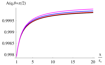
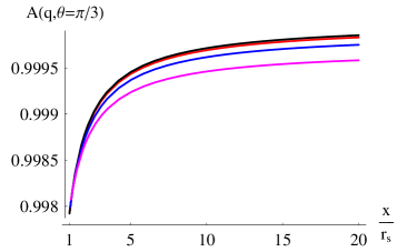
Figure 1: The plots depict the function $A(q,\theta;a)$ versus $x/r_{\text{s}}=\sqrt{q^{2}+a^{2}\cos^{2}\theta}/r_{\text{s}}$ for selected values of ($a/r_{\text{s}},\,\theta$) and $\tilde{k}=0.003$ has been constrained by the shadow observations (69). The black, red, blue, and magenta curves correspond to $a/r_{\text{s}}=0,\,0.3,\,0.6,\,0.9$, respectively. The black plot, corresponding to $a=0$, coincides with the plot of $A(q)=\Big{(}\frac{q-q_{+}}{q-q_{-}}\Big{)}^{\frac{k}{q_{+}-q_{-}}}$ (47).

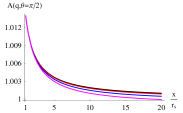
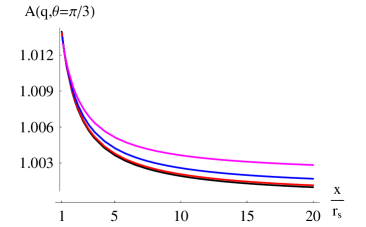
Figure 2: The plots depict the function $A(q,\theta;a)$ versus $x/r_{\text{s}}=\sqrt{q^{2}+a^{2}\cos^{2}\theta}/r_{\text{s}}$ for selected values of ($a/r_{\text{s}},\,\theta$) and $\tilde{k}=-0.02$ has been constrained by the shadow observations (69). The black, red, blue, and magenta curves correspond to $a/r_{\text{s}}=0,\,0.3,\,0.6,\,0.9$, respectively. The black plot, corresponding to $a=0$, coincides with the plot of $A(q)=\Big{(}\frac{q-q_{+}}{q-q_{-}}\Big{)}^{\frac{k}{q_{+}-q_{-}}}$ (47).

If we identify $B(q,\theta;a)$ with unity we obtain a rotating solution up to $a^{2}$, that is, $\mathcal{R}=\mathcal{O}(a^{2})+\cdots$ and the left-hand sides of the field equations,

$$\mathcal{R}\Big{(}\mathcal{R}_{\mu\nu}-\frac{1}{4}g_{\mu\nu}\mathcal{R}\Big{)}+(g_{\mu\nu}\square-\nabla_{\mu}\nabla_{\nu})\mathcal{R}=0,$$

are of the same order.

However, for the remaining section of this work we will not identify $B(q,\theta;a)$ with unity, nor rely on the numerical solutions depicted in Fig. 1 and 2, as for some interesting physical applications the exact form the conformal factor $A(q,\theta;a)$ is not needed. This is indeed the case when investigating the shadow of such rotating solutions as the null geodesic equations are separable for any $A(q,\theta;a)$.

VII Shadow

In order to investigate the shadow, it is better to rewrite the rotating metric (50) keeping the only function $r(q)$ and $\Delta(q)$:

$$ds^{2} =A(q,\theta;a)\Big{[}-\frac{\Delta-a^{2}\sin^{2}\theta}{\rho^{2}}dt^{2}+\frac{\rho^{2}}{\Delta}dq^{2}+\rho^{2}d\theta^{2}$$

$$+\frac{2a\sin^{2}\theta}{\rho^{2}}(\Delta-r^{2}-a^{2})dt\,d\phi+\frac{\Sigma}{\rho^{2}}\sin^{2}\theta d\phi^{2}\Big{]},$$ (52)

where $\rho^{2}(q,\theta)=r^{2}+a^{2}\cos^{2}\theta$ and $\Sigma(q,\theta)=(r^{2}+a^{2})^{2}-\Delta a^{2}\sin^{2}\theta$.

Separability of the equations of motion for massive and massless particles has been done for the case where $A(q,\theta;a)\equiv 1$ first in Azreg-Ainou-2014 then elsewhere. For the generic case where $A(q,\theta;a)$ is not constant, the separability of the equations of motion is only possible for null geodesics (massless particles), as shown in Junior . The equations describing the null geodesics are straightforwardly brought to the form

$$A^{2}\rho^{4}(\dot{q})^{2}= [E(r^{2}+a^{2})-aL]^{2}-\Delta[Q+(aE-L)^{2}],$$

$$\equiv E^{2}\mathbb{R}(q),$$ (53)

$$A^{2}\rho^{4}(\dot{\theta})^{2}= Q+a^{2}E^{2}\cos^{2}\theta-L^{2}\cot^{2}\theta\equiv E^{2}\Theta(\theta),$$ (54)

$$\dot{t}= \frac{E\Sigma}{A\rho^{2}\Delta}+\frac{aL(\Delta-r^{2}-a^{2})}{A\rho^{2}\Delta},$$ (55)

$$\dot{\phi}= \frac{L(\Delta-a^{2}\sin^{2}\theta)}{A\rho^{2}\Delta\sin^{2}\theta}-\frac{aE(\Delta-r^{2}-a^{2})}{A\rho^{2}\Delta},$$ (56)

where $E$ and $L$ are the energy and angular momentum, respectively, $Q$ is the Carter’s constant, and the dot denotes derivative with respect to proper time or affine parameter. In terms of the impact parameters $\eta\equiv Q/E^{2}$ and $\xi\equiv L/E$, the functions $\mathbb{R}(q)$ and $\Theta(\theta)$ take the form

$$\mathbb{R}(q)=[r^{2}+a^{2}-a\xi]^{2}-\mathcal{L}\Delta,$$ (57)

$$\Theta(\theta)=\mathcal{L}-(a\sin\theta-\xi\csc\theta)^{2},$$ (58)

$$\mathcal{L}\equiv\eta+(a-\xi)^{2}$$ (59)

Now, we require the presence of unstable spherical null geodesics obeying the constraints $\mathbb{R}(q)=0$ and $\mathbb{R}^{\prime}(q)=0$, where prime denotes derivative with respect to $q$, along with $\mathbb{R}^{\prime\prime}(q)>0$. This yields

$$\eta=\frac{r^{2}[8\Delta r^{\prime}(2a^{2}r^{\prime}+r\Delta^{\prime})-16\Delta^{2}(r^{\prime})^{2}-r^{2}(\Delta^{\prime})^{2}]}{a^{2}(\Delta^{\prime})^{2}},$$ (60)

$$\xi=\frac{r^{2}+a^{2}}{a}-\frac{2\Delta(r^{2})^{\prime}}{a\Delta^{\prime}}.$$ (61)

For the determination of the shadow, the celestial coordinates $x$ and $y$, which allow to span the observer’s sky, are defined for a distant observer by

$$x=\lim_{r\to\infty}\Big{[}-r^{2}\sin\theta\frac{d\phi}{dr}\Big{|}_{\theta=\theta_{i}}\Big{]}=\lim_{q\to\infty}\Big{[}-q^{2}\sin\theta\frac{d\phi}{dq}\Big{|}_{\theta=\theta_{i}}\Big{]},$$ (62)

$$y=\lim_{r\to\infty}\Big{[}r^{2}\frac{d\theta}{dr}\Big{|}_{\theta=\theta_{i}}\Big{]}=\lim_{q\to\infty}\Big{[}q^{2}\frac{d\theta}{dq}\Big{|}_{\theta=\theta_{i}}\Big{]},$$ (63)

where $\theta_{i}$ is the observer’s inclination. Using Eqs. (53), (54), (56) we obtain:

$$x= -\xi\csc\theta_{i},$$ (64)

$$y= \pm\sqrt{\eta+a^{2}\cos^{2}\theta_{i}-\xi^{2}\cot^{2}\theta_{i}}\,,$$

$$= \pm\sqrt{\mathcal{L}-(a\sin\theta_{i}-\xi\csc\theta_{i})^{2}}\,.$$ (65)

These last equations along with (60) and (61) will allow us to sketch the shape of the shadow angular size versus the dimensionless parameter $\tilde{k}=k/r_{s}$. From the static solution (47) we obtain

$$r_{s}=\frac{2M}{1+\tilde{k}},$$ (66)

which will allow us to express the functions of the rotating solution (48) and (49) in terms of $M$, $\tilde{k}$, and $a_{*}=a/M$.

Figure 3: The plot depicts the shadow angular size $\theta_{d}$ versus the dimensionless parameter $\tilde{k}$ assuming that M87* if modeled by the rotating metric (52). If $\tilde{k}=k/r_{s}\in[-0.129,\,0.004]$, then $\theta_{d}=42\pm 3\,\mu\text{as}$ EHT1 ; EHT2 ; EHT3 ; EHT4 . We took $M=6.5\times 10^{9}M_{\odot}$, $a_{*}\equiv a/M=0.5$, distance to Earth $D=16.8\,\text{Mpc}$, inclination $\theta_{i}=17^{\text{o}}$.

Figure 4: The plot depicts the shadow angular size $\theta_{d}$ versus the dimensionless parameter $\tilde{k}$ assuming that M87* if modeled by the rotating metric (52). If $\tilde{k}=k/r_{s}\in[-0.155,\,-0.033]$, then $\theta_{d}=42\pm 3\,\mu\text{as}$ EHT1 ; EHT2 ; EHT3 ; EHT4 . We took $M=6.5\times 10^{9}M_{\odot}$, $a_{*}\equiv a/M=0.94$, distance to Earth $D=16.8\,\text{Mpc}$, inclination $\theta_{i}=17^{\text{o}}$.

The shadow angular size $\theta_{d}$ is defined by

$$\theta_{d}=\frac{2R_{s}}{D},$$ (67)

where $D$ is the distance to Earth and $R_{s}$ is the radius of the circle that shares with the closed curve describing the shadow the following three points: The rightmost point of the shadow ($x=x_{r},\,y=0$), the upper- and lowermost points of the shadow ($x=x_{b},\,y=y_{\text{max}}$) and ($x=x_{b},\,y=-y_{\text{max}}$). These are the three red points of Figure 3 of Ref. Maeda where $\alpha$ denotes $x$ and $\beta$ denotes $y$:

$$R_{s}=\frac{(x_{r}-x_{b})^{2}+y_{\text{max}}^{2}}{2(x_{r}-x_{b})}.$$ (68)

Now, if the rotating metric (52) describes the central black hole M87* we must have $M=6.5\times 10^{9}M_{\odot}$, $a_{*}\equiv a/M\in[0.5,0.94]$, distance to Earth $D=16.8\,\text{Mpc}$, inclination $\theta_{i}=17^{\text{o}}$, and shadow angular size $\theta_{d}=42\pm 3\,\mu\text{as}$ EHT1 ; EHT2 ; EHT3 ; EHT4 . This yields the bounds for $\tilde{k}\in[-0.129,\,0.004]$ if $a_{*}=0.5$ and $\tilde{k}\in[-0.155,\,-0.033]$ if $a_{*}=0.94$, as shown in Fig. 3 and Fig. 4, respectively. These two bounds restrict $\tilde{k}$ by

$$-0.155\leq\tilde{k}\leq 0.004\,.$$ (69)

VIII Stability analysis

Upon comparing our action in the Einstein frame (40) with that in the same frame given in Eq. (2.10) of BRS23 , we make the following identification

$$M^{2}=\frac{8\Lambda}{\kappa},\quad\zeta=\sqrt{\frac{12\Lambda}{\kappa}}\,\ln\omega,\quad U(\zeta)=\frac{8\Lambda^{2}}{\kappa},$$ (70)

and $\rho\equiv 0$. If ($h_{\mu\nu},\,\delta\zeta$) denote the perturbations of the fields,

$$g_{\mu\nu}=\tilde{g}_{\mu\nu}+h_{\mu\nu},\qquad\zeta=\tilde{\zeta}+\delta\zeta,$$

where the tilde notation is used for the background fields in the Einstein frame, the field equations reduce to BRS23

$$\delta\tilde{G}_{\mu\nu}+\Lambda h_{\mu\nu}=0,\qquad\tilde{\square}(\delta\zeta)=0.$$ (71)

Since these are the same perturbation equations of general relativity in a de Sitter background in the presence of a scalar field which has led to the stability of the static Schwarzschild–de Sitter black hole against linear perturbations BRS20 , we conclude that our static solutions, regardless of the value of $\tilde{\mathcal{R}}$ ($\tilde{\mathcal{R}}=0$ or $\tilde{\mathcal{R}}\neq 0$), are also stable against linear perturbations. We could have reached the same conclusion upon applying the analysis given either in BRS20 ; Zerilli or in s4 .

Since the conformal factor is not given analytically, the stability of rotating solutions cannot be performed following the work done in BRS20 or any other reference. However, for small rotation parameter $a$ we may claim stability of rotating solutions by continuity.

We conclude that the non-rotating solution is stable against linear radial perturbations and we claim that the rotating solution is also stable as far as the rotating parameter remains small compared to the mass of the solution.

IX Conclusion

In this work we have emphasized the role of the Buchdahl parameter $k$, which has dimensions of length and is of higher-derivative nature. We have shown that the Buchdahl parameter $k$ can be considered as the scalar charge and should take on any in real value.

Upon making a recap of the general and special non-rotating Buchdahl-inspired metrics, we proceeded to transform the general non-rotating Buchdahl-inspired metric to a seed metric suitable for generalizing its rotating counterpart. Then we applied the non-complexification procedure of the Newman-Janis algorithm to reduce the number of unknown functions of the rotating metric to 1: This is the function $\psi$ in Eq. (45) or the function $A$ in Eq. (46).

After that, we specialized to the special metric having $\Lambda=0$ and obtained its exact rotating counterpart, Eqs. (49) & (50), up to a conformal factor $A$, which we could not determine analytically but numerically, upon solving the equation $\mathcal{R}=0$, as depicted in Figs. 1 & 2.

The shadow analysis of the exact rotating solution has shown that the reduced Buchdahl parameter $\tilde{k}$ could be restricted by $-0.155\leq\tilde{k}\leq 0.004$ (69).

Finally, we concluded that the non-rotating solution is stable against linear radial perturbations. The stability of the rotating solution cannot be performed as $A$ is not given analytically; however, we may claim that it is continuous too by continuity at least for small values of the rotation parameter compared to the mass of the solution.

- (1) T. Clifton, P. G. Ferreira, A. Padilla, and C. Skordis, Modified gravity and cosmology, Phys. Rept. 513 (2012) 1-189, arXiv:1106.2476 [astro-ph.CO]
- (2) A. De Felice and S. Tsujikawa, theories, Living Rev. Rel. 13 (2010) 3, arXiv:1002.4928 [gr-qc]
- (3) T. P. Sotiriou and V. Faraoni, Theories Of Gravity, Rev. Mod. Phys. 82 (2010) 451-497, arXiv:0805.1726 [gr-qc]
- (4) S. Nojiri and S. D. Odintsov, Unified cosmic history in modified gravity: from theory to Lorentz non-invariant models, Phys. Rept. 505 (2011) 59-144, arXiv:1011.0544 [gr-qc]
- (5) S. Capozziello, A. Stabile, and A. Troisi, Spherically symmetric solutions in gravity via Noether Symmetry Approach, Class. Quantum Grav.24:2153-2166 (2007); arXiv:gr-qc/0703067
- (6) L. Sebastiani and S. Zerbini, Static spherically symmetric solutions in gravity, Eur. Phys. J. C 71 (2011) 1591, arXiv:1012.5230 [gr-qc]
- (7) M. Gürses, T.C. Şişman, and B. Tekin, New exact solutions of quadratic curvature gravity, Phys. Rev. D 86 (2012) 024009, arXiv:1204.2215 [hep-th]
- (8) V. Pravda, A. Pravdová, J. Podolský, and R. Švarc, Exact solutions to quadratic gravity, Phys. Rev. D 95 (2017) 8, 084025, arXiv:1606.02646 [gr-qc]
- (9) H. A. Buchdahl, Non-linear Lagrangians and cosmological theory, Mon. Not. Roy. Astron. Soc. 150 (1970) 1
- (10) H. A. Buchdahl, On the Gravitational Field Equations Arising from the Square of the Gaussian Curvature, Nuovo Cimento, Vol. 23, No 1, 141 (1962)
- (11) H. K. Nguyen, Beyond Schwarzschild-de Sitter spacetimes: I. A new exhaustive class of metrics inspired by Buchdahl for pure gravity in a compact form, Phys. Rev. D 106, 104004 (2022), arXiv:2211.01769 [gr-qc]
- (12) K. A. Bronnikov, G. Clément, C. P. Constantinidis, and J. C. Fabris, Structure and stability of cold scalar-tensor black holes, Phys. Lett. A 243, 121 (1998), arXiv:gr-qc/9801050; K. A. Bronnikov, G. Clément, C. P. Constantinidis, and J. C. Fabris, Cold Scalar-Tensor Black Holes: Causal Structure, Geodesics, Stability, Grav. Cosmol. 4, 128 (1998), arXiv:gr-qc/9804064
- (13) K. A. Bronnikov, Scalar-tensor theory and scalar charge, Acta Phys. Polon. B 4, 251 (1973), Link to pdf
- (14) T. Matsuda, On the gravitational collapse in Brans–Dicke theory of gravity, Prog. Theor. Phys. 47, 738 (1972)
- (15) M. Campanelli and C. Lousto, Are Black Holes in Brans–Dicke Theory precisely the same as in General Relativity?, Int. J. Mod. Phys. D 2, 451 (1993) , arXiv:gr-qc/9301013
- (16) H. K. Nguyen, Beyond Schwarzschild-de Sitter spacetimes: II. An exact non-Schwarzschild metric in pure gravity and new anomalous properties of spacetimes, Phys. Rev .D 107, 104008 (2023), arXiv:2211.03542 [gr-qc]
- (17) M. Azreg-Aïnou, Regular and conformal regular cores for static and rotating solutions, Phys. Lett. B D 730, 95 (2014), arXiv:1401.0787 [gr-qc]
- (18) M. Azreg-Aïnou, From static to rotating to conformal static solutions: Rotating imperfect fluid wormholes with(out) electric or magnetic field, Phys. Eur. Phys. J. C 74, 2865 (2014), arXiv:1401.4292 [gr-qc]
- (19) M. Azreg-Aïnou, Generating rotating regular black hole solutions without complexification, Phys. Rev. D 90, 064041 (2014), arXiv:1405.2569 [gr-qc]
- (20) H. K. Nguyen, Nontriviality of asymptotically flat Buchdahl-inspired metrics in pure gravity, arXiv:2305.12037 [gr-qc]
- (21) H. K. Nguyen and M. Azreg-Aïnou, Traversable Morris-Thorne-Buchdahl wormholes in quadratic gravity, Eur. Phys. J. C 83 (2023) 626, arXiv:2305.04321 [gr-qc]
- (22) H. K. Nguyen and M. Azreg-Aïnou, New insights into Weak Energy Condition and wormholes in Brans-Dicke gravity, arXiv:2305.15450 [gr-qc]
- (23) D. F. Carneiro, E. A. Freiras, B. Gonçalves, A. G. de Lima, and I. L. Shapiro, On useful conformal transformations in General Relativity, Grav. Cosmol. 10, 305 (2004), arXiv:gr-qc/0412113
- (24) H. C. D. Lima Junior, L. C. B. Crispino, P. V. P. Cunha and C. A. R. Herdeiro, Spinning black holes with a separable Hamilton–Jacobi equation from a modified Newman–Janis algorithm, Eur. Phys. J. C 80, 1036 (2020), https://link.springer.com/article/10.1140/epjc/s10052-020-08572-w
- (25) K. Hioki and K. Maeda, Measurement of the Kerr Spin Parameter by Observation of a Compact Object’s Shadow, Phys. Rev. D 80, 024042 (2009), https://link.springer.com/article/10.1140/epjc/s10052-020-08572-w
- (26) Event Horizon Telescope Collaboration, K. Akiyama et al., First M87 Event Horizon Telescope Results. I. The Shadow of the Supermassive Black Hole, Astrophys. J. Lett. 875, L1, (2019), http://arxiv.org/abs/1906.11238
- (27) Event Horizon Telescope Collaboration, K. Akiyama et al., First M87 Event Horizon Telescope Results. IV. Imaging the Central Supermassive Black Hole, Astrophys. J. Lett. 875, L4, (2019), http://arxiv.org/abs/1906.11241
- (28) Event Horizon Telescope Collaboration, K. Akiyama et al., First M87 Event Horizon Telescope Results. V. Physical Origin of the Asymmetric Ring, Astrophys. J. Lett. 875, L5, (2019), http://arxiv.org/abs/1906.11242
- (29) Event Horizon Telescope Collaboration, K. Akiyama et al., First M87 Event Horizon Telescope Results. VI. The Shadow and Mass of the Central Black Hole, Astrophys. J. Lett. 875, L6, (2019), http://arxiv.org/abs/1906.11243
- (30) S. Boudet, M. Rinaldi, and S. Silveravalle, On the stability of scale-invariant black holes, J. High Energy Phys. 01, 133, (2023), arXiv:2211.06110 [gr-qc]
- (31) C. Dioguardi and M. Rinaldi, A note on the linear stability of black holes in quadratic gravity, Eur. Phys. J. Plus 135, 920, (2020), arXiv:2007.11468 [gr-qc]
- (32) F.J. Zerilli, Effective potential for even-Parity Regge–Wheeler gravitational perturbation equations, Phys. Rev. Lett. 24, 737, (1970)
- (33) K. A. Bronnikov and S. G. Rubin, Black holes, cosmology and extra dimensions, 2nd edition, World Scientific, Singapore, 2022