Big Bang initial conditions and self-interacting hidden dark matter
Abstract
A variety of supergravity and string models involve hidden sectors where the hidden sectors may couple feebly with the visible sectors via a variety of portals. While the coupling of the hidden sector to the visible sector is feeble its coupling to the inflaton is largely unknown. It could couple feebly or with the same strength as the visible sector which would result in either a cold or a hot hidden sector at the end of reheating. These two possibilities could lead to significantly different outcomes for observables. We investigate the thermal evolution of the two sectors in a cosmologically consistent hidden sector dark matter model where the hidden sector and the visible sector are thermally coupled. Within this framework we analyze several phenomena to illustrate their dependence on the initial conditions. These include the allowed parameter space of models, dark matter relic density, proton-dark matter cross section, effective massless neutrino species at BBN time, self-interacting dark matter cross-section, where self-interaction occurs via exchange of dark photon, and Sommerfeld enhancement. Finally fits to the velocity dependence of dark matter cross sections from galaxy scales to the scale of galaxy clusters is given. The analysis indicates significant effects of the initial conditions on the observables listed above. The analysis is carried out within the framework where dark matter is constituted of dark fermions and the mediation between the visible and the hidden sector occurs via the exchange of dark photons. The techniques discussed here may have applications for a wider class of hidden sector models using different mediations between the visible and the hidden sectors to explore the impact of Big Bang initial conditions on observable physics.
1 Introduction
Hidden sectors appear in most modern models of particle physics beyond the standard model and have become increasingly relevant in analyses of particle physics phenomena. Success of precision electroweak physics tell us that the hidden sector couplings to the standard model must be feeble. But what about the coupling of the hidden sector to the inflaton? If the coupling of the hidden sector to the inflaton is also feeble relative to the coupling of the standard model the population of the hidden sector particles would be negligible and their temperature would be much colder than of the standard model particles. On the other extreme the hidden sector and the visible sectors could couple democratically, i.e.,with equal strength, to the inflaton and thus be essentially in thermal equilibrium at the end of reheating. These cases represent two extreme possibilities with a variety of other possibilities in between. Because of the interactions between the visible and the hidden sectors, the two sectors are thermally coupled and thus their evolution is constrained by the initial condition on the hidden sector at the end of inflation which can be codified by the ratio , where is the temperature of the hidden sector and is the temperature of the visible sector initially after reheating. It is thus of relevance to ask the influence of the initial conditions on physical observables at low energy. In this work we study the effect of on a variety of physical observables, i.e., on the relic density of dark matter, on the proton-DM scattering cross-sections, on the number of massless degrees of freedom at BBN, and on DM self-interaction cross-sections. For DM self-interaction cross-section, we further analyze the effect of on its velocity dependence and on Sommerfeld enhancement and analyze the effect of on fits to the galactic dark matter cross sections from the scale of dwarf galaxies to the scale of galaxy clusters. The portal we utilize in the analysis consists of a hidden sector with a gauge invariance with kinetic mixing[1] and Stueckelberg mass growth of the gauge boson [2]. By numerically solving the Schrödinger equation, we are able to achieve a comprehensive understanding of the dark matter self-interacting cross-section in this model. While our analysis is done in a specific choice of the portal one may expect similar effects discussed in this work using other portals connecting visible and the hidden sectors.
The outline of the rest of the note is as follows: Section 2 gives a summary of the thermal evolution of coupled visible and hidden sectors while section 3 discusses a specific model with the visible sector coupled to one hidden sector where the coupling arises via kinetic mixing along with Stueckelberg mass generation for the hidden sector gauge boson. Section 4 discusses the effect of on dark freeze-out and on the relic density of dark matter. Here we also discuss the dependence of at BBN time on and further the effect of on the allowed parameter space and on spin-independent proton-DM cross section. In section 5 we discuss the effect of on Sommerfeld enhancement for the self-interacting dark matter cross section. In section 6 we discuss the effect of on fits to the galaxy data on dark matter cross sections from low relative velocities to high relative velocities which encompass scales from dwarf galaxies to galaxy clusters. Conclusions are given in section 7. Additional details related to the analysis are given in sections 8-10. Further, in section 11 we give a comparison of our analysis of the thermal evolution when the total entropy is conserved vs the thermal evolution when the entropies of the visible and the hidden sectors are separately conserved. In this section we also analyze the accuracy of using conservation of total entropy in computations of yields for dark matter since in general the total entropy is not conserved unless the sectors equilibrate.
2 Cosmologically consistent evolution of coupled visible and hidden sectors in DM analysis.
As mentioned in the previous section, most models of particle physics based on physics beyond the standard model contain hidden sectors which may be feebly coupled to the visible sector. In this case the thermal evolution of each is interdependent on the other. Thus the approximation typically made that the entropy of the visible and the hidden sectors are separately conserved is invalid. Further, the hidden sector by itself may consist of several sectors some of which may interact directly with the visible sector while others indirectly via their interactions with other hidden sectors which couple with the visible sector. First, in this case the Hubble expansion is affected by the hidden sectors via their energy densities so that
| (2.1) |
where is the energy density of the visible sector and the energy density of the -th hidden sector where have temperature dependence so that
| (2.2) |
and the total entropy density of the visible and hidden sectors is given by
| (2.3) |
Here and are the energy and entropy degrees of freedom and are temperature dependent. A full expression for them for the specific model we will consider is given in section 3. In [3] an analysis was given where the visible sector (V) at temperature is coupled to the hidden sector at temperature , the hidden sector is coupled to the hidden sector at temperature , and so on and finally that the hidden sector at temperature is coupled to the hidden sector at temperature . In the analysis of [3] radiation dominance was assumed. Here we extend the analysis to include radiation and matter. In this case the energy densities for various sectors obey the following set of coupled Boltzmann equations
| (2.4) |
Here and are the energy and momentum densities for the sector , and where refers to the visible sector, and to the hidden sectors, and where encodes in it all the possible processes exchanging energy between neighboring sectors. We note now that the total energy density in an expanding universe satisfies the equation
| (2.5) |
where is the total pressure density. In the analysis it is convenient to introduce the functions and , where for radiation dominance and for matter dominance. More generally and are temperature dependent and this dependence is taken into account in the evolution equations. Thus and satisfy the evolution equations
| (2.6) | |||
| (2.7) |
We use the visible sector temperature as the clock as thus wish to write the evolution equations Eqs. (2.6) and (2.7) in terms of temperature rather than time. This is accomplished using the relation
| (2.8) |
Thus using , one has
| (2.9) |
Next decomposing so that , one finds that can be written as
| (2.10) |
Here
| (2.11) |
where and is defined so that
| (2.12) |
Note that one may also write
| (2.13) |
Here , where and . Thus we have an equation for which takes the form
| (2.14) |
where . Eqs. (2.14) give us a set of differential equations for the evolution functions . These have to be solved along with the Boltzmann equations governing the number density evolution of the hidden sector particles. This will allow us to determine the relic densities of all stable species and describe the thermal evolution of this coupled system. For the case of the visible sector coupled to one hidden sector we have , , , , and we define . The source term is discussed in section 8. With this notation specific to the case of the visible sector and one hidden sector we have the following equation for which governs the temperature evolution of the hidden sector relative to that of the visible sector
| (2.15) |
We note that and are pre-calculated and we use tabulated results from micrOMEGAs [4]. As noted already and for the hidden sector that enter Eq. (2.2) and Eq. (2.3) are temperature dependent [5, 6] and their explicit expressions are given in Eq.(9.4).
3 The model coupling visible and hidden sectors
There are a variety of portals that allow communication between the visible and the hidden sectors. These include the Higgs field portal [7], kinetic mixing of two gauge fields [1], Stueckelberg mass mixing [2, 8], kinetic and Stueckelberg mass mixing [9], Higgs-Stueckelberg portal[10], as well as other possibilities such as higher dimensional operators. In this work we focus on kinetic mixing along with the mass growth for the hidden sector gauge field via the Stueckelberg mechanism. Thus for analysis in this work we consider a specific model for dark matter which is an extension of the standard model with an gauge invariance where the gauge field has kinetic mixing with the visible sector gauge field [1] and in general a Stueckelberg mass mixings [2, 9, 11, 12]. We assume that the hidden sector has a dark fermion which interacts with the gauge field. Thus the extended Lagrangian consisting of the SM part and the extended part is given by
| (3.1) |
Here is the gauge field for the , is the gauge field of , is an axionic field which gives mass to and is absorbed in the unitary gauge and is the dark fermion where is the charge of and is gauge coupling of . Further, is the kinetic mixing parameter between the field strengths of and , and and are the Stueckelberg mass parameters. A non-vanishing will lead to a milli-charge for the dark fermion and we assume neutrality of dark matter and thus set in the analysis333A non-vanishing was used to resolve the EDGES anomaly in the analysis of [13].. The spontaneous breaking of the electroweak symmetry along with the Stueckelberg mass growth gives rise to mixing among the three gauge fields where is the third component of the gauge field of the standard model. The mixings give rise to a mass square matrix which can be diagonalized by the three Euler angles which are given in Eq.(9.3). The diagonalization gives the following mass eigenstates: the boson, a massive dark photon and the massless photon . The Lagrangian governing the interaction of dark photon and dark fermion which enters into our analysis is given by
| (3.2) |
The interaction of Eq. 3.2 involves two massive gauge bosons (). For the case when the kinetic mixing is small one has and which is negligible. In addition the dark photon will have couplings with the standard model quarks and leptons which are discussed in Appendix 10. Setting , the input parameters of the model are which are what appear in Table 1. We note here that models with the vector boson as the mediator between the hidden sector and the visible sector have been considered in several previous works [14, 15, 16, 17, 18, 19, 20, 21, 22, 23, 24, 25, 26, 27, 28, 29, 30, 31, 32, 33, 34, 35, 36, 37, 38, 39, 40, 41, 42, 43, 44, 45, 46, 47, 48, 49, 50, 51, 52, 53, 54, 55, 56]. Axions and dark photons in the light to ultralight mass region have also been investigated [45, 57, 58, 47, 59, 60, 61], and dark photons have been used in explaining astro-physical phenomena including galactic -rays [62, 63] and PAMELA positron excess [64, 65, 66, 67, 68].
We further note that the dark photon in this model even when very light and kinematically disallowed to decay into will eventually decay via the modes and and not contribute to dark matter density unless its lifetime is larger than the lifetime of the universe and even in that case only if it has non-negligible relic density, which is not the case we consider. Thus the dark fermion will be the only constituent of dark matter. Further details about this model is given in Appendix 9.
4 Big Bang constraints on dark freeze-out, relic density, , and on proton-DM cross-section
In this section we discuss the effects on the relic density, on the number of relativistic degrees of freedom due to the hidden sector at the BBN time, on the allowed parameter space of models, and on proton-dark matter scattering scattering cross section arising from different choices of the initial value at the end of reheating. In the model discussed in the preceding section, the dark fermion constitutes dark matter and has self-interactions due to exchange of dark photon.
4.1 Effect of on dark freeze-out and on relic density
In the analysis here we will discuss the effect of on the dark freeze-out which generates the relic density of . Computationally the quantities of interest for this purpose are the yields for the dark fermion and for the dark photon , where the yield is defined so that where is the number density and is the entropy density. Assuming conservation of total entropy (this assumption will be tested in section 11) the evolution equations for and are given by
| (4.1) | ||||
| (4.2) |
Here is the annihilation cross-section of into standard model particles which are denoted by , is their annihilation into dark photon while gives the annihilation of standard model particles into a dark photon, and and are the number densities of the fermion and the dark photon . In the above the cross-section for the process is given by
| (4.3) |
while the rest of the cross-sections are given in appendix of [13]. Here are Mandelstam variables where , and are matrix elements of which diagonalizes the mass and kinetic energy matrices of Eq.(3.1) as given in [9]. Further, we note that in addition to we also have which enters in the yield equations when kinematically allowed and is related to so that
| (4.4) |
In the above equation, the thermally averaged cross section and decay widths are given by
| (4.5) | ||||
| (4.6) |
The equilibrium yield of the i-th particle is given by
| (4.7) |
where is the entropy density. In Eqs.(4.5), (4.6) and (4.7), and are the modified Bessel functions of the second kind and of degrees one and of degree two. Further, cross sections for the processes , where are the standard model particles, can be found in Appendix D of [69]. As noted above in this model the dark photon is unstable and decays and does not contribute to the relic density and the entire DM relic density arises from the dark fermion where at current times the relic density is given by
| (4.8) |
where is the current entropy density, which is at current times can be gotten using Eqs. (2.15), (4.1) and (4.2), is the critical energy density needed to close the universe, and is defined so that km s-1 Mpc-1, where is the Hubble parameter today.
The procedure for solving the evolution equations involves simultaneous analysis of coupled equations Eq.(2.1)-Eq.(2.3), Eq.(2.15), Eq.(9.4), Eq.(9.5), the yield equations for , , Eq.(4.1)-Eq.(4.2), and Eqs.(4.3)-(4.8). Using these we do Monte Carlo simulations with parameters varying in the ranges
| (4.9) |
and search for model points satisfying all the current experimental constraints.
Table 1 gives 6 model points used in this paper
all of which are consistent with the current experimental constraints
[70] including those from a variety of experiments, i.e.,
BaBar [71, 72], HPS [73], LHCb [74], Belle-2 [75], SHiP [76], SeaQuest [77, 78] and NA62 [78],
CHARM [78], Cal [78, 79, 80], E137 [81], E141 [82], NA64 [83], NA48 [84]. For a sub-MeV dark photon mass stringent constraints arise from Supernova SN1987A [85] and from BBN, stellar cooling [86] and from the decay to on cosmological timescales [87, 30]
An analysis of these constraints in limiting the parameter space have been analyzed in[70, 69]. The parameter space chosen in the
current analysis is consistent with these constraints. In fact, a larger variation in
| No. | (in ) | (yrs) | |||
|---|---|---|---|---|---|
| (a) | 0.354 | 0.306 | 0.00738 | 3.99 | |
| (b) | 0.259 | 0.214 | 0.00675 | 6.29 | |
| (c) | 0.281 | 0.550 | 0.00931 | 400 | |
| (d) | 0.170 | 0.225 | 0.00618 | 19.3 | |
| (e) | 0.156 | 0.285 | 0.00631 | 52.9 | |
| (f) | 0.568 | 0.445 | 0.00810 | 2.62 |
We note here that the mass of the dark photon is in the sub MeV region and is long lived with its most dominant decay mode being . For kinetic mixing the decay width for the mode is given by [30, 87, 88]
| (4.10) |
where , is the kinetic mixing parameter of coupling between dark photon and photon given by as defined in [9], is the dark photon mass and is the electron mass. The dark photon lifetimes for the different model points are given in Table (1). Here we find that the dark photon lifetimes are smaller than the age of the universe and thus there is no contribution of the dark photon to the relic density and consequently no constraint on the allowed parameter space regarding the relic density constraint. We note, however, that even if the dark photon was long lived with a lifetime greater than the lifetime of the universe, its contribution to the relic density would be negligible. A recent analysis [69] in accord with the analysis of [30] shows that with one hidden sector it is not possible to get both a long lived dark photon which can contribute to the relic density and simultaneously achieve a significant amount of dark matter relic density. To do that one needs at least a two hidden sector model[69] in which a dark photon as dark matter can produce a non-negligible amount of dark matter.
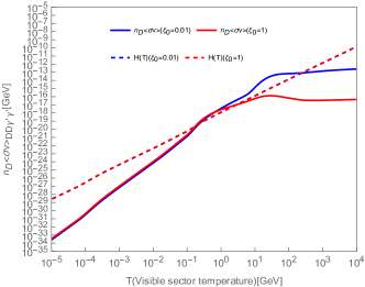
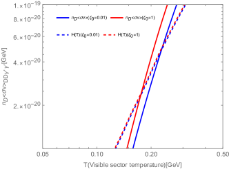
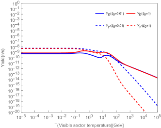
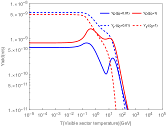
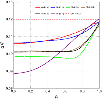
We discuss now the dependence of the dark matter freeze-out and of the relic density on the initial conditions. In the top left panel of Fig. 1 we exhibit the dependence of the dark freeze-out and specifically the decoupling of the dark photon and the dark fermion on where we consider the cases: and . The top right panel is the zoom in of the top right in the region of the freeze-out. From Fig. 1 we see that the process falls below H(T) at different temperatures for and for and consequently the temperature where the dark freeze-out occurs changes by a significant amount. The sensitivity of the freeze-out on directly affects the yields as shown in the bottom left panel and the bottom right panel (a zoom in of the bottom left panel) of Fig. 1. In the left panel of Fig. 2 we exhibit the dependence of the relic density on for the six model points of Table 1. Here we find that the relic density can change up to 40% as varies in the range .
4.2 Dependence of at BBN on
One of the predictions of beyond the standard model physics is , the number of effective relativistic degrees of freedom at BBN. For the standard model . The current experimental constraint on is summarized in Fig. 39 of the Planck Collaboration [89] which shows the spread in . Thus the Planck Collaboration gives while the joint BBN analysis of deuterium/helium abundance and the Planck CMB data gives . Here we will use the conservative constraint on so that . In the model under discussion, the dark fermion D and dark photon will contribute to the effective neutrino number. Such contribution is given by
| (4.11) |
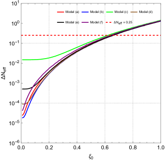
where can computed from Eq.(9.4) and Eq.(4.11) is to be evaluated at the BBN temperature MeV (for related works see, e.g., [90, 91]). In Table 2, is computed for the six model points of Table 1 for and while the right panel of Fig. 2 exhibits for the six model points for in the range . The analysis in general indicates that hidden sectors which start off cooler than the standard model at the end of reheating contribute a smaller amount to than those which are relatively hotter at the end of reheating. Further, the analysis indicates that models where could accommodate more massless degrees of freedom allowing for the possibility of building a wider class of models with more hidden sector particles which may still be consistent with the constraint at BBN time.
| Model | ||||
|---|---|---|---|---|
| (a) | 1.50 | 0.692 | 1.53E-5 | 0.0391 |
| (b) | 1.36 | 0.675 | 1.22E-5 | 0.0369 |
| (c) | 1.53 | 0.700 | 1.18E-2 | 0.208 |
| (d) | 1.40 | 0.679 | 6.37E-5 | 0.0558 |
| (e) | 1.43 | 0.684 | 3.80E-4 | 0.0873 |
| (f) | 1.42 | 0.685 | 2.59E-5 | 0.0448 |
4.3 Effect of on the allowed parameter space and on spin-independent proton-DM cross section
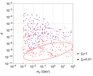
Next, we investigate the influence of on the allowed parameter space consistent for a chosen range of relic density. To this end we constrain the relic density to lie in the range and to lie in the range of 5 GeV to 10 TeV. Specifically we explore the allowed region for the two cases: and . The result of our analysis is exhibited in the left panel of Fig. 3 which gives a scatter plot of the allowed models in vs where those with color blue correspond to and those with color red correspond to . One of the interesting result that emerges is that for most of the models lie in the range while for the allowed range is . Thus, the analysis shows that the initial choice of significantly impacts the model’s allowed parameter space.
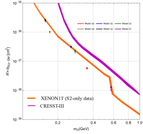
also has significant effect on the proton-DM scattering cross section in the direct detection experiments for dark matter. Specifically we consider the spin independent proton-DM cross section . Here we use the micrOMEGAs[4] to find the spin independent cross section. In the right panel of Fig. 3 we exhibit for the six model points of Table 1 and their dependence on in the range (0.01-1) is indicated by the small vertical lines for each of the model points. The numerical values of the for and are exhibited in Table 3 for the models of Table 1. Here one finds that the variation of the cross-section can be as large as 40%. Thus some of the models that are eliminated for the case would still be viable for the case .
| Model | ||
|---|---|---|
| (cm2) | (cm2) | |
| (a) | 5.84E-38 | 5.24E-38 |
| (b) | 3.18E-37 | 2.87E-37 |
| (c) | 2.19E-37 | 1.81E-37 |
| (d) | 1.03E-36 | 8.88E-37 |
| (e) | 2.61E-36 | 2.23E-36 |
| (f) | 1.39E-38 | 1.03E-38 |
5 Self-interacting dark matter, Sommerfeld enhancement, and dependence on
The self-interacting dark matter cross sections arises from the processess , , and via the exchange of a dark photon. The Lagrangian of Eq. (3.1) leads to a Yukawa potential between the D-fermions due to the dark photon exchange in the non-relativistic limit so that
| (5.1) |
where the plus sign is for and and the minus sign is for . In some of the regions of parameters (i.e. ), tree-level scattering or the Born approximation is no longer valid and one has contributions from higher order dark photon exchanges as shown in Fig. 4 which contribute to scattering. In this case we need to numerically solve the Schrodinger equation to find the accurate scattering cross sections. The radial equation one needs to solve is given by
| (5.2) |
where is the particle momentum and is the potential. The substitution and gives[94]
| (5.3) |
The non-perturbative effect arising from the repeated exchange of the mediator is often encoded in Sommerfeld enhancement and has been discussed in several previous works (see, e.g.,[95, 96, 97, 98, 36, 24] and the references therein). Thus including non-perturbative effects the annihilation cross section times the velocity (where is the relative velocity in the CM system) for the cross section for the elastic scattering process may be written as
| (5.4) |
where is the tree level cross section and is the Sommerfeld enhancement. As noted in the present context the contribution to the Sommerfeld enhancement arises from multiple exchanges of the dark photon . The solution of the differential equation Eq.(5.3) has the form:
| (5.5) |
where is the phase shift for the th partial wave. We write the Sommerfeld enhancement of -th partial wave cross-section for the case of the Yukawa potential so that
| (5.6) |
where [94], . Using Eq. (5.5), we get
| (5.7) |
Taking larger than 30 gives a good enough approximation to the exact solution. Typically an attractive potential leads to Sommerfeld enhancement of cross section at low collision velocities, but one may also have Sommerfeld suppression for a repulsive potential.
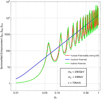
In the left panel of Fig. 5 we exhibit Sommerfeld enhancement for the case of a negative Yukawa potential. Here we see that Sommerfeld enhancement can be very significant and further the enhancement shows oscillatory behavior with . To check the accuracy of our numerical analysis and to explain the oscillatory behavior we compare our result with those from the Hulthen potential as an approximation to the Yukawa potential for which one can obtain a good analytic approximation for the S-wave. The Hulthen potential is given by[99, 100]
| (5.8) |
It is known that Hulthen potential is a very good approximation to Yukawa potential both at short and at long distances. With it one can find an analytic solution for the S-wave and thus find a good analytic approximation to the S-wave Sommerfeld enhancement [101, 102]:
| (5.9) |
From Eq.(5.9), valid for the attractive potential case, it is obvious that the oscillation is due to the existence of the cosine term. For the Coulomb potential the Sommerfeld enhancement for the S-wave is given by
| (5.10) |
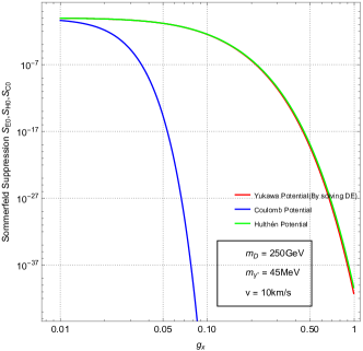
where plus is for repulsive potential and minus is for attractive potential. The left panel of Fig.5 gives a comparison of the S-wave Sommerfeld effect for three different potentials: Yukawa, Hulthen and Coulomb. The analysis shows that Hulthen potential gives a good approximation to the Yukawa potential and also explains the deep oscillations as a function of . For the case of a repulsive potential ( negative), the analysis is very different. A comparison of the numerical analysis using Yukawa potential and the analytic solution using Hulthen potential for the case of a repulsive potential is given in the right panel of Fig. 5. Here again one finds that the numerical analysis and the Hulthen potential result fully agree.
Having checked the numerical accuracy of our analysis in Fig. 5
we next investigate the effect of the Big Bang initial conditions on
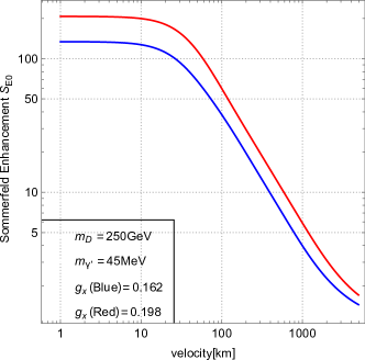
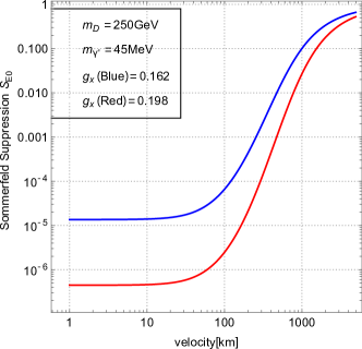
Sommerfeld enhancement. In Fig. 6 we compare S-wave Sommerfeld enhancement for the cases
and for the case of an attractive Yukawa potential.
The left panel of Fig. 6 shows Sommerfeld enhancement vs
and here one finds that (red) gives an enhancement which is
larger than for the case (blue). In the analysis we keep the relic density fixed at for = 0.01 and 1 by allowing
to vary.
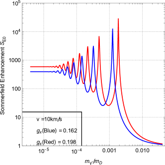
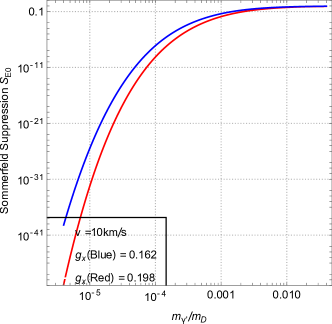
The right panel of
Fig. 6 displays Sommerfeld enhancement as a function of and here one finds that the oscillation peaks for the case
(red) are significantly larger than those for the case (blue).
A similar analysis for a repulsive Yukawa potential is carried out in
Fig. 7. However, in this case we have
Sommerfeld suppression rather than an enhancement where the
Sommerfeld suppression is vs for the left panel and vs
for the right panel and
the red curve is for and the blue curve for .
For both cases the Sommerfeld suppression is significantly larger
for relative to .
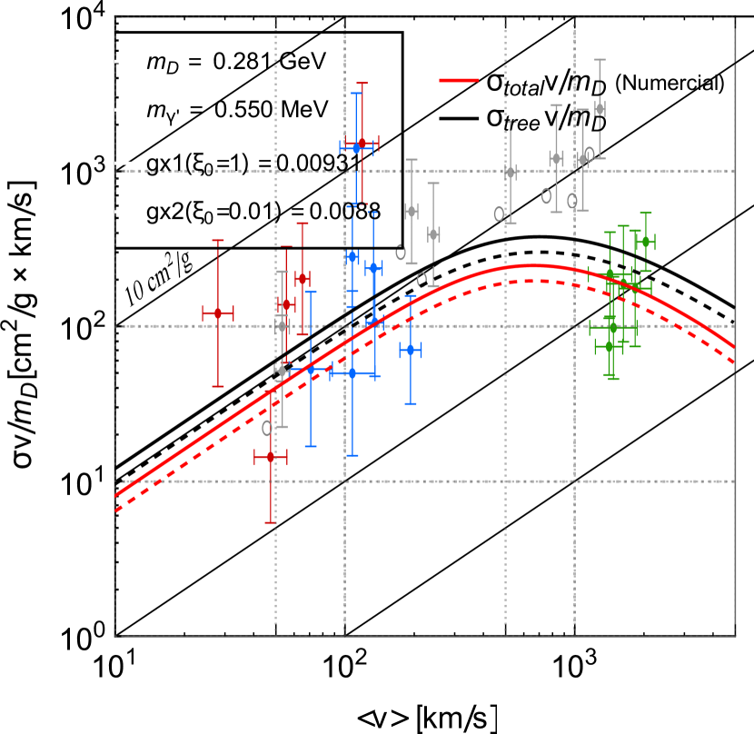
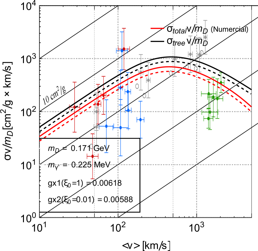
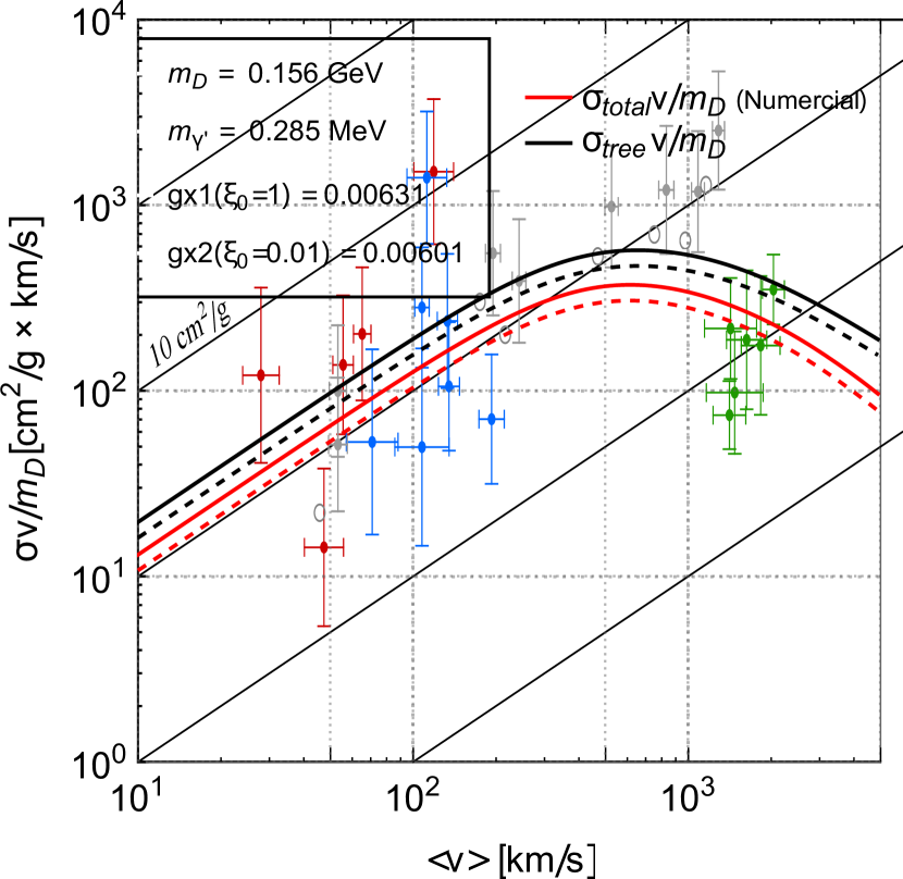
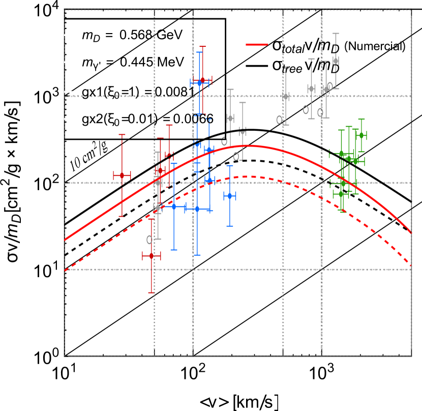
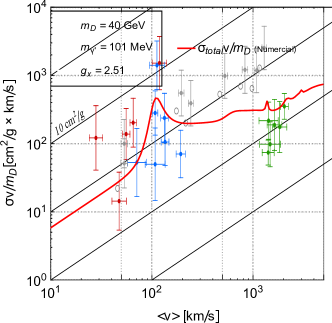
6 Effect of on fit to galaxy data
Several analyses of galaxy data indicate that dark matter is collisional at the scale of dwarf galaxies and appears collision-less at the scale of galaxy clusters[33, 38, 103]. Thus, for dwarf galaxies one finds collisional velocity of dark matter in the range 10-100 km/s and 1 cm2/g cm2/g [103, 33] where is the cross section and is the mass of DM particle. For midsize galaxies such as the low surface brightness galaxies (LSB) and the Milky Way one finds in the range 80-200 km/s and 0.5 cm2/g cm2/g. The galaxy clusters exhibit km/s. Here it is estimated that the is maximally 1 cm2/g [103, 33, 104] and could be as low as 0.065 cm2/g cm2/g [105, 38, 106]. As is well known one interesting possibility to account for the velocity dependence of the DM cross sections is that DM is self-interacting by Spergel and Steinhardt [107] and there is considerable follow up work on this idea [108, 109, 110, 111, 112, 113, 114, 115, 22, 25, 26, 27, 28, 36]. An analysis of fit to the data within the dark photon model was previously done in [11] (see also [116, 117]). Here we study the dependence of the fits on . Further, here the analysis goes beyond the Born approximation used in [11] taking into account non-perturbative effects encoded in the Sommerfeld enhancement with also inclusion of identical particle exchange effects. Since the dark matter is constituted of dark Dirac fermions consisting of and constituents, we will have processes of the type , and . Thus the total cross section is given by
| (6.1) |
where the factor of arises due to identical nature of particles.
To numerically calculate the cross section, we start with Eq.(5.3) and use the method of [27]. Here in the computation of DM cross sections, we need to calculate the phase shifts () for separately from the phase shifts () for while the phase shifts for the process will be the same as for the process . Including all contributions, i.e., from , and , and taking account of the identical nature of particles in and scattering we find
| (6.2) |
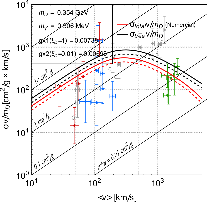
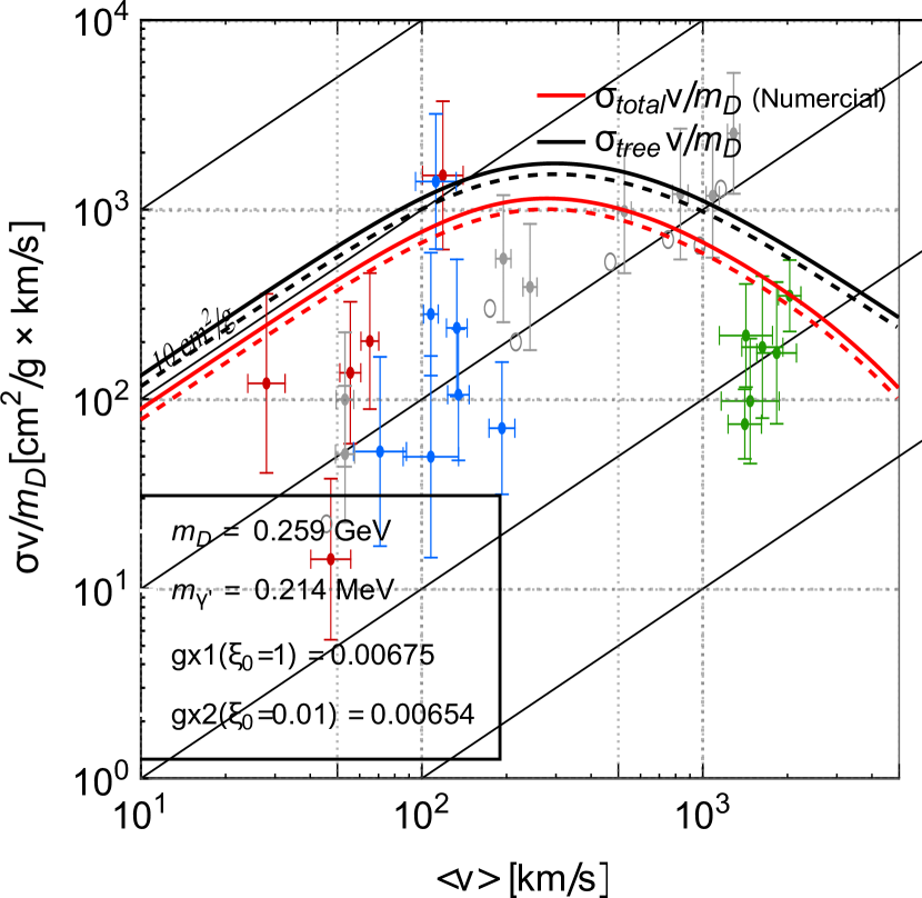
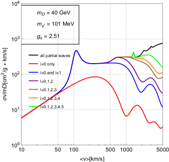
where and . The details leading to Eq.(6.2) are given in section 10. The result of our numerical analysis to fit the galaxy data on in the range of velocities from 10 km/s to km/s is given in Fig. 8 which exhibits the dependence of the fits on in the range to . In the analysis we allow to vary to keep the relic density fixed at as varies between 0.01 and 1. The analysis shows that the variation of with is significant and can sometimes be as large as (see Model (f)) in Fig. 8. We note that the plots include Sommerfeld enhancement effects but these effects are relatively small. The reason for it is that the Sommerfeld enhancement strongly depends on as can be seen from the left panel of Fig. 5. However, in the analysis of galaxy fits of Fig. 8, we find that is relatively small which suppresses the Sommerfeld enhancement. Our result here is consistent with a similar observation on Sommerfeld enhancement in the work of [36] (see also [24]). In Fig. 8 the Born approximation results are also plotted for comparison with the exact solutions. Further, we note that more fine tuned fits to the galaxy data can be gotten by adjustment of the model parameters such that resonances appear in some of the low lying partial waves, e.g., S, P and D waves. This is exhibited in Fig. 9 where in the left panel we see enhancements in the S and the P waves appear to simulate the oscillations in the data at km/s and at km/s. On the right panel of Fig. 9, we plot the cross section contributed from each partial wave separately. It is clear that the peak at km/s is largely due to the S-wave while the one at km/s has a large contribution from although sum of all partial waves up to enter in the fit given on the left panel.
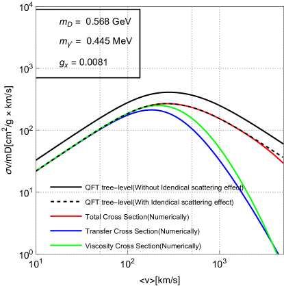
Besides the total cross section, transfer cross section [118, 22, 23, 25, 26, 27, 28] () which have been used in the simulations of long range interactions [108, 111, 119]. Further, viscosity cross sections () are also widely considered in analysis of SIDM[27, 120, 121]. They are defined so that
| (6.3) |
In terms of partial waves and are given by
| (6.4) | ||||
| (6.5) | ||||
| (6.6) | ||||
| (6.7) |
Details of their computation in terms of partial waves are given in section 10. Fig. 10 shows that differ significantly from each other. We also exhibit the tree level cross section for comparison.
7 Conclusion
Hidden sectors are ubiquitous in models of extra dimensions, in extended supergravity and in strings and appear in a variety of beyond the standard model constructions such as in moose/quiver gauge theories (see, e.g., [122, 123, 124, 125]). While the hidden sectors are neutral under the standard model gauge group they can couple feebly with the standard model. However, the couplings of the hidden sector to the inflaton could vary over a wide range. Thus on one extreme the hidden sector coupling to the inflaton could be negligible relative to the coupling of the standard model. In this case at the end of reheating there would be essentially no production of the hidden sector particles, except via gravitational production, and the hidden sector would likely be colder than the standard model. On the other extreme the hidden sector and the visible sectors could couple democratically to the inflaton and in this case the hidden sector and the visible sectors would be in thermal equilibrium at the end of reheating. These two extremes would have significantly different thermal evolution and would result in significant differences in their predictions of the physical observables. In this work we have investigated these effects in the context of a specific hidden sector model which arises from a extension of the standard model gauge group. The contents of the hidden sector consists of a dark fermion which has gauge interactions with the gauge field. The communication between the hidden sector and the visible sector arises from kinetic mixing between the and gauge fields where the gauge field acquires mass via the Stueckelberg mechanism. In view of the asymmetric coupling of the visible and the hidden sectors to the inflaton field, the temperature of the hidden sector and of the visible sector will in general be unequal at the end of reheating. Thus the ratio of the two, i.e., enters in the thermal evolution of the hidden and the visible sectors and affects phenomena at low energy.
The analysis of the work provides a cosmologically consistent
framework in that it involves a synchronous evolution of the coupled hidden and visible sectors.
In the above framework we investigate a number of phenomena and their dependence on . These include dark freeze-out, relic density
and the extra number of relativistic degrees of freedom at the
BBN time, and the proton-DM cross-section. Further, we investigate
the effects of on the self-interaction
cross section and on Sommerfeld enhancement.
The model is then used in fitting self-interacting dark matter cross sections from galaxy scales to the scale of galaxy clusters. Here we find that fits to data show a significant variation sometime as much as for in the range . Thus the analysis indicates that inclusion of hidden sectors
which appear in a variety of models of particle physics beyond the standard model, the initial constraints on the hidden sector at the end of reheating and specifically on could have significant influence on observables and thus their inclusion will be relevant for accurate description of physical phenomena.
While our analysis is done for the case of one portal, the general techniques
discussed here would be valid for a broader class of models.
Finally, we show that the approximation often made in
the thermal evolution of visible and hidden sectors by assuming
entropy conservation for each of the sectors separately
gives widely inaccurate results even for the case for very feeble
interactions such as, for example, with the kinetic mixing parameter as low as . Such an analysis is thus a poor approximation to the analysis we carry out for the thermal evolution of the
visible and the hidden sectors in a synchronous manner using
Eq.(2.15). For generality we also consider the case with the mass mixing parameter which reaches a similar conclusion.
We have also analyzed the accuracy of assuming the conservation of total entropy
for the yield equations and find that the differences between conservation assumption
and no conservation assumption are typically within . We conclude that
an accurate thermal evolution is essential for the current and future precision analyses in cosmology while analyzing physics involving hidden sectors.
Acknowledgments: Discussions with Amin Abou Ibrahim and Zhuyao Wang are acknowledged. The research of JL and PN was supported in part by the NSF Grant PHY-2209903.
8 Appendix A: Source functions
9 Appendix B: Model details
In addition to the interactions given in section 3, there are interactions involving the dark sector and the standard model particles in the canonical basis where the kinetic energy and the mass matrices of the gauge boson are diagonal. Here the standard model fermions (i.e., quarks and leptons) have feeble interactions with the dark photon which are given by
| (9.1) |
where is the gauge coupling constant, stands for the standard model fermions and angle is defined in Eq.(9.3). The vector and axial vector couplings of the dark photon with the SM fermions are given by
| (9.2) | ||||
Here , is the third component of isospin, and is the electric charge for the fermion . The angles and which along with are the three Euler angles with diagonalize the gauge boson mass square matrix involving the fields are defined as [9]
| (9.3) |
where . For the model of Eq.(3.1) where the hidden sector consists of the dark photon and a dark Dirac fermion, and are given by
| (9.4) |
where , .
Further, to compute , we need and , which are given by
| (9.5) |
Here and . For total , we need energy and pressure densities for both the visible and the hidden sectors and we use the relation
| (9.6) |
Before proceeding further we note that the extension to include both the kinetic and mass mixings in Eqs.(3.2)-(9.3) is straightforward as has been discussed in [9] and we exhibit them here for easy reference to guide the discussion in section 7. With inclusion of both the kinetic mixing parameter and the mass mixing parameter , the neutral current Lagrangian in the hidden sector takes the form
| (9.7) |
where
| (9.8) |
where is defined so that . There is also a corresponding modification of the neutral current in the visible sector as discussed in [9]. The constraints on and arising from the fits to the electroweak data are mild and one finds that can be as large as 0.05 consistent with the same level of fits to the electroweak data as the standard model[9].
10 Self-interacting dark matter cross sections
10.1
Let us first consider scattering. Here the wave function for scattering of a plane wave scattering from a central potential is given by . In this case the scattering amplitude has an expansion in terms of the partial wave amplitudes where is the phase shift for the l-th partial wave so that has the expansion and have the expansion
| (10.1) |
The transfer cross-section is defined by
| (10.2) |
Using the relations
| (10.5) |
the transfer cross section can be written as
| (10.6) |
The viscosity cross-section defined by
| (10.7) |
can be expanded in terms of partial waves using the relations
| (10.11) |
which gives
| (10.12) |
10.2 ,
Here the scattering involves identical particles which are fermions so the overall wave function for the particles must be anti-symmetric. This can happen in two ways: (i) spin anti-symmetric and space symmetric or (ii) spin symmetric and space anti-symmetric. Now the two spin particles can have a total spin 1 (triplet state) or total spin is zero (singlet state). For the triplet state the space wave function must be anti-symmetric in and for the singlet state the space wave function must be symmetric. Thus we have for the expression
| (10.13) |
Further, is given by
| (10.14) |
where the front factor of is to take account of the identical nature of the scattering particles. The partial wave analysis of gives
| (10.15) |
Here since the potential governing scattering is different from the one that governs scattering. Similar calculations are done for transfer cross section and for viscosity cross section. Further, .
11 Entropy conservation approximation
Here in subsection 11.1 we will discuss the validity of separate entropy conservation approximation for visible and hidden sectors and in subsection 11.2 we will discuss the validity of the conservation of the total entropy which is the sum of the visible and the hidden sector entropies.
11.1 On the validity of separate entropy conservation approximation of visible and hidden sector
In several previous works (see, e.g.,[29]) an assumption of entropy conservation per co-moving volume separately for the visible and the hidden sectors is made to relate at different temperatures. The above implies that the ratio is unchanged at different temperatures where and are the entropy densities for the visible and the hidden sectors where
| (11.1) |
Specifically it is assumed that the following relation between the temperatures and holds
| (11.2) |
Noting that and where we can write the above equation as follows
| (11.3) |
Note that the left hand side is a highly non-linear function of since for our model
| (11.4) |
where
and .
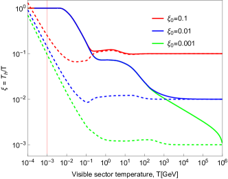
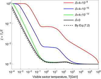
In Fig. 11 we give a comparison of the analysis of the evolution of the using Eq.(2.15) vs the evolution given by the approximation of entropy conservation in co-moving volume for the visible and the hidden sectors separately. The analysis shows that as gets progressively smaller deviations of the approximate solutions gets progressively worse and especially in the freeze-in region where , the deviations of the approximate from the exact is huge for temperatures in the visible sector below GeV. More importantly for any choice of in the range which includes both the freeze-out and the freeze-in regions, the prediction of for the approximation is always inaccurate at the BBN temperature of MeV. The right panel gives a plot of as a function of the visible sector temperature for different values of for the case when . Here one finds that the approximation (dashed line) gives reasonably accurate result for the case when , i.e., there is no kinetic mixing but it gives highly inaccurate results for the case when in non-vanishing, even as small as .
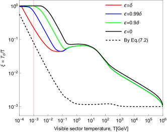
In the analysis done so far we assumed . For generality we consider now the case where we include the mass mixing parameter along with kinetic mixing . Thus we discuss again the thermal evolution when there are both kinetic mixing and mass mixing present where we use the relations given by Eq.(9.7) and Eq.(9.8) and related relations given in [9]. In Fig. 12 we investigate the effect of including along on the evolution of . The left panel is for the case with and as expected the evolution for different shows a pattern similar to the left panel of Fig. 11. The right panel of Fig. 12 shows that evolutions with different follow a similar path at high temperatures but begin to separate at GeV. This separation results in significantly different values of at BBN temperature. As expected we find that since and together control the thermal evolution, there is a significant difference in the pattern of evolution here relative to those of Fig. 11. However, for both Fig. 11 and Fig. 12 one finds that the predictions for given by the approximation equation Eq.(11.2) shown by dashed curves differs by wide margins from the result using Eq.(2.15) over wide regions of the parameter space and specifically at BBN temperature. Thus, our conclusion, is that the entropy conservation approximation separately for the visible and hidden sectors in thermal evolution is not suitable for a precision analysis.
11.2 On the validity of the total entropy conservation
In the preceding analysis we discussed the evolution of for the case when entropy conservation per comoving volume is assumed separately for the visible and the hidden sectors vs the case when the entropy conservation is assumed only for their sum. It is found that the deviations between the two analysis could be significant, as exhibited by Fig. (11) and Fig.(12). It is then pertinent to ask the validity of conservation of total entropy since the total entropy itself in not conserved either unless various sectors themselves equillibrate. We note that in our analysis the deduction of the evolution equation for did not involve any assumptions related to entropy and the only place where the conservation of the total entropy was used was in the yield equations. For this reason we reconsider the Botzmann equation for the yields without the assumption of total entropy conservation. We focus on the yield equation for the -fermion which constitutes dark matter in the model and the analysis for the yield for the dark photon is very similar.
Thus we start with the Boltzmann equation for the number density which is given by
| (11.5) |
We note now that the equation for the yield without the use of entropy conservation gives so that
| (11.6) |
We notice that the set of terms on the right-hand side of Eq.(11.6) involving are exactly what we have in Eq.(4.1). Further, the term involving vanishes on using the conservation of total entropy and indicates the deviation of the exact equation from the approximate one where total entropy conservation is assume. A similar analysis holds for the case of the dark photon yield equation. Thus we carry out an analysis using the exact equations without entropy conservation constraint and compare it with the analysis where entropy conservation is assumed. Results are presented in Fig.(13).
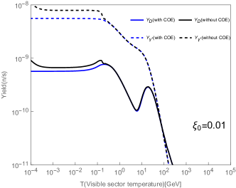
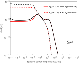
The analysis of Fig.(13) shows, when the conservation of entropy (COE) is dropped, the results do not change a lot. Thus the top left panel for shows that the yield changes by typically within without inclusion of the entropy conservation constraint. A similar analysis holds for the case as shown on the right panel of Fig.(13). However, we point out an issue that arises at very low temperatures. Without COE constraint the yields begin to exhibit an instability at low temperature at around GeV. In part this could be due to lack of analytic expressions for the entropy degrees of freedom in the visible sector where on relies on curves or tabulated data (see, e.g.,[5, 6]) because of hadronization of quarks and gluons. The instability arises essentially from the terms proportional to . A proper analysis of this issue is outside the scope of this work and a relevant topic for further investigation.
References
- [1] B. Holdom, Phys. Lett. B 166, 196-198 (1986) doi:10.1016/0370-2693(86)91377-8
- [2] B. Kors and P. Nath, Phys. Lett. B 586, 366-372 (2004) doi:10.1016/j.physletb.2004.02.051 [arXiv:hep-ph/0402047 [hep-ph]].
- [3] A. Aboubrahim and P. Nath, JHEP 09, 084 (2022) doi:10.1007/JHEP09(2022)084 [arXiv:2205.07316 [hep-ph]].
- [4] G. Bélanger, F. Boudjema, A. Goudelis, A. Pukhov and B. Zaldivar, Comput. Phys. Commun. 231, 173-186 (2018) doi:10.1016/j.cpc.2018.04.027 [arXiv:1801.03509 [hep-ph]].
- [5] M. Hindmarsh and O. Philipsen, Phys. Rev. D 71, 087302 (2005) doi:10.1103/PhysRevD.71.087302 [arXiv:hep-ph/0501232 [hep-ph]].
- [6] L. Husdal, Galaxies 4, no.4, 78 (2016) doi:10.3390/galaxies4040078 [arXiv:1609.04979 [astro-ph.CO]].
- [7] B. Patt and F. Wilczek, [arXiv:hep-ph/0605188 [hep-ph]].
- [8] B. Kors and P. Nath, JHEP 07, 069 (2005) doi:10.1088/1126-6708/2005/07/069 [arXiv:hep-ph/0503208 [hep-ph]].
- [9] D. Feldman, Z. Liu and P. Nath, Phys. Rev. D 75, 115001 (2007) doi:10.1103/PhysRevD.75.115001 [arXiv:hep-ph/0702123 [hep-ph]].
- [10] M. Du, Z. Liu and P. Nath, Phys. Lett. B 834, 137454 (2022) doi:10.1016/j.physletb.2022.137454 [arXiv:2204.09024 [hep-ph]].
- [11] A. Aboubrahim, W. Z. Feng, P. Nath and Z. Y. Wang, Phys. Rev. D 103, no.7, 075014 (2021) doi:10.1103/PhysRevD.103.075014 [arXiv:2008.00529 [hep-ph]].
- [12] A. Aboubrahim and P. Nath, Phys. Rev. D 99, no.5, 055037 (2019) doi:10.1103/PhysRevD.99.055037 [arXiv:1902.05538 [hep-ph]].
- [13] A. Aboubrahim, P. Nath and Z. Y. Wang, JHEP 12, 148 (2021) doi:10.1007/JHEP12(2021)148 [arXiv:2108.05819 [hep-ph]].
- [14] X. Chen and S. H. H. Tye, JCAP 06, 011 (2006) doi:10.1088/1475-7516/2006/06/011 [arXiv:hep-th/0602136 [hep-th]].
- [15] D. Feldman, B. Kors and P. Nath, Phys. Rev. D 75, 023503 (2007) doi:10.1103/PhysRevD.75.023503 [arXiv:hep-ph/0610133 [hep-ph]].
- [16] D. Feldman, Z. Liu and P. Nath, AIP Conf. Proc. 939, no.1, 50-58 (2007) doi:10.1063/1.2803786 [arXiv:0705.2924 [hep-ph]].
- [17] K. Cheung and T. C. Yuan, JHEP 03, 120 (2007) doi:10.1088/1126-6708/2007/03/120 [arXiv:hep-ph/0701107 [hep-ph]].
- [18] W. Z. Feng, P. Nath and G. Peim, Phys. Rev. D 85, 115016 (2012) doi:10.1103/PhysRevD.85.115016 [arXiv:1204.5752 [hep-ph]].
- [19] D. Feldman, P. Fileviez Perez and P. Nath, JHEP 01, 038 (2012) doi:10.1007/JHEP01(2012)038 [arXiv:1109.2901 [hep-ph]].
- [20] W. Z. Feng, A. Mazumdar and P. Nath, Phys. Rev. D 88, no.3, 036014 (2013) doi:10.1103/PhysRevD.88.036014 [arXiv:1302.0012 [hep-ph]].
- [21] X. Chen, JCAP 09, 029 (2009) doi:10.1088/1475-7516/2009/09/029 [arXiv:0902.0008 [hep-ph]].
- [22] M. R. Buckley and P. J. Fox, Phys. Rev. D 81, 083522 (2010) doi:10.1103/PhysRevD.81.083522 [arXiv:0911.3898 [hep-ph]].
- [23] M. Ibe and H. b. Yu, Phys. Lett. B 692, 70-73 (2010) doi:10.1016/j.physletb.2010.07.026 [arXiv:0912.5425 [hep-ph]].
- [24] J. L. Feng, M. Kaplinghat, H. Tu and H. B. Yu, JCAP 07, 004 (2009) doi:10.1088/1475-7516/2009/07/004 [arXiv:0905.3039 [hep-ph]].
- [25] A. Loeb and N. Weiner, Phys. Rev. Lett. 106, 171302 (2011) doi:10.1103/PhysRevLett.106.171302 [arXiv:1011.6374 [astro-ph.CO]].
- [26] S. Tulin, H. B. Yu and K. M. Zurek, Phys. Rev. Lett. 110, no.11, 111301 (2013) doi:10.1103/PhysRevLett.110.111301 [arXiv:1210.0900 [hep-ph]].
- [27] S. Tulin, H. B. Yu and K. M. Zurek, Phys. Rev. D 87, no.11, 115007 (2013) doi:10.1103/PhysRevD.87.115007 [arXiv:1302.3898 [hep-ph]].
- [28] K. Schutz and T. R. Slatyer, JCAP 01, 021 (2015) doi:10.1088/1475-7516/2015/01/021 [arXiv:1409.2867 [hep-ph]].
- [29] J. L. Feng, H. Tu and H. B. Yu, JCAP 10, 043 (2008) doi:10.1088/1475-7516/2008/10/043 [arXiv:0808.2318 [hep-ph]].
- [30] J. Redondo and M. Postma, JCAP 02, 005 (2009) doi:10.1088/1475-7516/2009/02/005 [arXiv:0811.0326 [hep-ph]].
- [31] X. Chu, T. Hambye and M. H. G. Tytgat, JCAP 05, 034 (2012) doi:10.1088/1475-7516/2012/05/034 [arXiv:1112.0493 [hep-ph]].
- [32] X. Chu, Y. Mambrini, J. Quevillon and B. Zaldivar, JCAP 01, 034 (2014) doi:10.1088/1475-7516/2014/01/034 [arXiv:1306.4677 [hep-ph]].
- [33] M. Kaplinghat, S. Tulin and H. B. Yu, Phys. Rev. Lett. 116, no.4, 041302 (2016) doi:10.1103/PhysRevLett.116.041302 [arXiv:1508.03339 [astro-ph.CO]].
- [34] R. T. D’Agnolo and J. T. Ruderman, Phys. Rev. Lett. 115, no.6, 061301 (2015) doi:10.1103/PhysRevLett.115.061301 [arXiv:1505.07107 [hep-ph]].
- [35] E. Kuflik, M. Perelstein, N. R. L. Lorier and Y. D. Tsai, Phys. Rev. Lett. 116, no.22, 221302 (2016) doi:10.1103/PhysRevLett.116.221302 [arXiv:1512.04545 [hep-ph]].
- [36] T. Bringmann, F. Kahlhoefer, K. Schmidt-Hoberg and P. Walia, Phys. Rev. Lett. 118, no.14, 141802 (2017) doi:10.1103/PhysRevLett.118.141802 [arXiv:1612.00845 [hep-ph]].
- [37] J. A. Evans, C. Gaidau and J. Shelton, JHEP 01, 032 (2020) doi:10.1007/JHEP01(2020)032 [arXiv:1909.04671 [hep-ph]].
- [38] L. Sagunski, S. Gad-Nasr, B. Colquhoun, A. Robertson and S. Tulin, JCAP 01, 024 (2021) doi:10.1088/1475-7516/2021/01/024 [arXiv:2006.12515 [astro-ph.CO]].
- [39] N. Fernandez, Y. Kahn and J. Shelton, JHEP 07, 044 (2022) doi:10.1007/JHEP07(2022)044 [arXiv:2111.13709 [hep-ph]].
- [40] K. Kaneta, H. S. Lee and S. Yun, Phys. Rev. Lett. 118, no.10, 101802 (2017) doi:10.1103/PhysRevLett.118.101802 [arXiv:1611.01466 [hep-ph]].
- [41] K. Kaneta, H. S. Lee and S. Yun, Phys. Rev. D 95, no.11, 115032 (2017) doi:10.1103/PhysRevD.95.115032 [arXiv:1704.07542 [hep-ph]].
- [42] R. T. Co, A. Pierce, Z. Zhang and Y. Zhao, Phys. Rev. D 99, no.7, 075002 (2019) doi:10.1103/PhysRevD.99.075002 [arXiv:1810.07196 [hep-ph]].
- [43] J. A. Dror, K. Harigaya and V. Narayan, Phys. Rev. D 99, no.3, 035036 (2019) doi:10.1103/PhysRevD.99.035036 [arXiv:1810.07195 [hep-ph]].
- [44] P. Agrawal, N. Kitajima, M. Reece, T. Sekiguchi and F. Takahashi, Phys. Lett. B 801, 135136 (2020) doi:10.1016/j.physletb.2019.135136 [arXiv:1810.07188 [hep-ph]].
- [45] A. J. Long and L. T. Wang, Phys. Rev. D 99, no.6, 063529 (2019) doi:10.1103/PhysRevD.99.063529 [arXiv:1901.03312 [hep-ph]].
- [46] G. Alonso-Álvarez, T. Hugle and J. Jaeckel, JCAP 02, 014 (2020) doi:10.1088/1475-7516/2020/02/014 [arXiv:1905.09836 [hep-ph]].
- [47] Y. Nakai, R. Namba and Z. Wang, JHEP 12, 170 (2020) doi:10.1007/JHEP12(2020)170 [arXiv:2004.10743 [hep-ph]].
- [48] G. Choi, T. T. Yanagida and N. Yokozaki, JHEP 01, 057 (2021) doi:10.1007/JHEP01(2021)057 [arXiv:2008.12180 [hep-ph]].
- [49] C. Delaunay, T. Ma and Y. Soreq, JHEP 02, 010 (2021) doi:10.1007/JHEP02(2021)010 [arXiv:2009.03060 [hep-ph]].
- [50] P. W. Graham, J. Mardon and S. Rajendran, Phys. Rev. D 93, no.10, 103520 (2016) doi:10.1103/PhysRevD.93.103520 [arXiv:1504.02102 [hep-ph]].
- [51] Y. Ema, K. Nakayama and Y. Tang, JHEP 07, 060 (2019) doi:10.1007/JHEP07(2019)060 [arXiv:1903.10973 [hep-ph]].
- [52] A. Ahmed, B. Grzadkowski and A. Socha, JHEP 08, 059 (2020) doi:10.1007/JHEP08(2020)059 [arXiv:2005.01766 [hep-ph]].
- [53] J. Berger, K. Jedamzik and D. G. E. Walker, JCAP 11, 032 (2016) doi:10.1088/1475-7516/2016/11/032 [arXiv:1605.07195 [hep-ph]].
- [54] M. Ibe, S. Kobayashi, Y. Nakayama and S. Shirai, JHEP 04, 009 (2020) doi:10.1007/JHEP04(2020)009 [arXiv:1912.12152 [hep-ph]].
- [55] S. D. McDermott and S. J. Witte, Phys. Rev. D 101, no.6, 063030 (2020) doi:10.1103/PhysRevD.101.063030 [arXiv:1911.05086 [hep-ph]].
- [56] A. Fradette, M. Pospelov, J. Pradler and A. Ritz, Phys. Procedia 61, 689-693 (2015) doi:10.1016/j.phpro.2014.12.081
- [57] I. M. Bloch, R. Essig, K. Tobioka, T. Volansky and T. T. Yu, JHEP 06, 087 (2017) doi:10.1007/JHEP06(2017)087 [arXiv:1608.02123 [hep-ph]].
- [58] M. Pospelov, A. Ritz and M. B. Voloshin, Phys. Rev. D 78, 115012 (2008) doi:10.1103/PhysRevD.78.115012 [arXiv:0807.3279 [hep-ph]].
- [59] J. E. Kim and D. J. E. Marsh, Phys. Rev. D 93, no.2, 025027 (2016) doi:10.1103/PhysRevD.93.025027 [arXiv:1510.01701 [hep-ph]].
- [60] L. Hui, J. P. Ostriker, S. Tremaine and E. Witten, Phys. Rev. D 95, no.4, 043541 (2017) doi:10.1103/PhysRevD.95.043541 [arXiv:1610.08297 [astro-ph.CO]].
- [61] J. Halverson, C. Long and P. Nath, Phys. Rev. D 96, no.5, 056025 (2017) doi:10.1103/PhysRevD.96.056025 [arXiv:1703.07779 [hep-ph]].
- [62] C. Boehm, D. Hooper, J. Silk, M. Casse and J. Paul, Phys. Rev. Lett. 92, 101301 (2004) doi:10.1103/PhysRevLett.92.101301 [arXiv:astro-ph/0309686 [astro-ph]].
- [63] C. Boehm and P. Fayet, Nucl. Phys. B 683, 219-263 (2004) doi:10.1016/j.nuclphysb.2004.01.015 [arXiv:hep-ph/0305261 [hep-ph]].
- [64] D. Feldman, Z. Liu and P. Nath, Phys. Rev. D 79, 063509 (2009) doi:10.1103/PhysRevD.79.063509 [arXiv:0810.5762 [hep-ph]].
- [65] N. Arkani-Hamed, D. P. Finkbeiner, T. R. Slatyer and N. Weiner, Phys. Rev. D 79, 015014 (2009) doi:10.1103/PhysRevD.79.015014 [arXiv:0810.0713 [hep-ph]].
- [66] M. Pospelov, A. Ritz and M. B. Voloshin, Phys. Lett. B 662, 53-61 (2008) doi:10.1016/j.physletb.2008.02.052 [arXiv:0711.4866 [hep-ph]].
- [67] L. Bergstrom, T. Bringmann, I. Cholis, D. Hooper and C. Weniger, Phys. Rev. Lett. 111, 171101 (2013) doi:10.1103/PhysRevLett.111.171101 [arXiv:1306.3983 [astro-ph.HE]].
- [68] L. Bergstrom, T. Bringmann and J. Edsjo, Phys. Rev. D 78, 103520 (2008) doi:10.1103/PhysRevD.78.103520 [arXiv:0808.3725 [astro-ph]].
- [69] A. Aboubrahim, W. Z. Feng, P. Nath and Z. Y. Wang, JHEP 06, 086 (2021) doi:10.1007/JHEP06(2021)086 [arXiv:2103.15769 [hep-ph]].
- [70] A. Aboubrahim, M. M. Altakach, M. Klasen, P. Nath and Z. Y. Wang, JHEP 03, 182 (2023) doi:10.1007/JHEP03(2023)182 [arXiv:2212.01268 [hep-ph]].
- [71] J. P. Lees et al. [BaBar], Phys. Rev. Lett. 113, no.20, 201801 (2014) doi:10.1103/PhysRevLett.113.201801 [arXiv:1406.2980 [hep-ex]].
- [72] J. P. Lees et al. [BaBar], Phys. Rev. Lett. 119, no.13, 131804 (2017) doi:10.1103/PhysRevLett.119.131804 [arXiv:1702.03327 [hep-ex]].
- [73] N. Baltzell et al. [HPS], Nucl. Instrum. Meth. A 859, 69-75 (2017) doi:10.1016/j.nima.2017.03.061 [arXiv:1612.07821 [physics.ins-det]].
- [74] R. Aaij et al. [LHCb], Phys. Rev. Lett. 124, no.4, 041801 (2020) doi:10.1103/PhysRevLett.124.041801 [arXiv:1910.06926 [hep-ex]].
- [75] E. Kou et al. [Belle-II], PTEP 2019, no.12, 123C01 (2019) [erratum: PTEP 2020, no.2, 029201 (2020)] doi:10.1093/ptep/ptz106 [arXiv:1808.10567 [hep-ex]].
- [76] C. Ahdida et al. [SHiP], Eur. Phys. J. C 81, no.5, 451 (2021) doi:10.1140/epjc/s10052-021-09224-3 [arXiv:2011.05115 [hep-ex]].
- [77] A. Berlin, S. Gori, P. Schuster and N. Toro, Phys. Rev. D 98, no.3, 035011 (2018) doi:10.1103/PhysRevD.98.035011 [arXiv:1804.00661 [hep-ph]].
- [78] Y. D. Tsai, P. deNiverville and M. X. Liu, Phys. Rev. Lett. 126, no.18, 181801 (2021) doi:10.1103/PhysRevLett.126.181801 [arXiv:1908.07525 [hep-ph]].
- [79] J. Blumlein and J. Brunner, Phys. Lett. B 701, 155-159 (2011) doi:10.1016/j.physletb.2011.05.046 [arXiv:1104.2747 [hep-ex]].
- [80] J. Blümlein and J. Brunner, Phys. Lett. B 731, 320-326 (2014) doi:10.1016/j.physletb.2014.02.029 [arXiv:1311.3870 [hep-ph]].
- [81] S. Andreas, C. Niebuhr and A. Ringwald, Phys. Rev. D 86, 095019 (2012) doi:10.1103/PhysRevD.86.095019 [arXiv:1209.6083 [hep-ph]].
- [82] E. M. Riordan, M. W. Krasny, K. Lang, P. De Barbaro, A. Bodek, S. Dasu, N. Varelas, X. Wang, R. G. Arnold and D. Benton, et al. Phys. Rev. Lett. 59, 755 (1987) doi:10.1103/PhysRevLett.59.755
- [83] D. Banerjee et al. [NA64], Phys. Rev. D 101, no.7, 071101 (2020) doi:10.1103/PhysRevD.101.071101 [arXiv:1912.11389 [hep-ex]].
- [84] J. R. Batley et al. [NA48/2], Phys. Lett. B 746, 178-185 (2015) doi:10.1016/j.physletb.2015.04.068 [arXiv:1504.00607 [hep-ex]].
- [85] J. H. Chang, R. Essig and S. D. McDermott, JHEP 01, 107 (2017) doi:10.1007/JHEP01(2017)107 [arXiv:1611.03864 [hep-ph]].
- [86] H. An, M. Pospelov and J. Pradler, Phys. Lett. B 725, 190-195 (2013) doi:10.1016/j.physletb.2013.07.008 [arXiv:1302.3884 [hep-ph]].
- [87] R. Essig, E. Kuflik, S. D. McDermott, T. Volansky and K. M. Zurek, JHEP 11, 193 (2013) doi:10.1007/JHEP11(2013)193 [arXiv:1309.4091 [hep-ph]].
- [88] S. D. McDermott, H. H. Patel and H. Ramani, Phys. Rev. D 97, no.7, 073005 (2018) doi:10.1103/PhysRevD.97.073005 [arXiv:1705.00619 [hep-ph]].
- [89] N. Aghanim et al. [Planck], Astron. Astrophys. 641, A6 (2020) [erratum: Astron. Astrophys. 652, C4 (2021)] doi:10.1051/0004-6361/201833910 [arXiv:1807.06209 [astro-ph.CO]].
- [90] T. Hasegawa, N. Hiroshima, K. Kohri, R. S. L. Hansen, T. Tram and S. Hannestad, JCAP 12, 012 (2019) doi:10.1088/1475-7516/2019/12/012 [arXiv:1908.10189 [hep-ph]].
- [91] M. Kawasaki, K. Kohri and N. Sugiyama, Phys. Rev. Lett. 82, 4168 (1999) doi:10.1103/PhysRevLett.82.4168 [arXiv:astro-ph/9811437 [astro-ph]].
- [92] A. H. Abdelhameed et al. [CRESST], Phys. Rev. D 100, no.10, 102002 (2019) doi:10.1103/PhysRevD.100.102002 [arXiv:1904.00498 [astro-ph.CO]].
- [93] E. Aprile et al. [XENON], Phys. Rev. Lett. 123, no.24, 241803 (2019) doi:10.1103/PhysRevLett.123.241803 [arXiv:1907.12771 [hep-ex]].
- [94] R. Iengo, JHEP 05, 024 (2009) doi:10.1088/1126-6708/2009/05/024 [arXiv:0902.0688 [hep-ph]].
- [95] M. Lattanzi and J. I. Silk, Phys. Rev. D 79, 083523 (2009) doi:10.1103/PhysRevD.79.083523 [arXiv:0812.0360 [astro-ph]].
- [96] N. Arkani-Hamed, D. P. Finkbeiner, T. R. Slatyer and N. Weiner, Phys. Rev. D 79, 015014 (2009) doi:10.1103/PhysRevD.79.015014 [arXiv:0810.0713 [hep-ph]].
- [97] S. Cassel, J. Phys. G 37, 105009 (2010) doi:10.1088/0954-3899/37/10/105009 [arXiv:0903.5307 [hep-ph]].
- [98] M. Cirelli, A. Strumia and M. Tamburini, Nucl. Phys. B 787, 152-175 (2007) doi:10.1016/j.nuclphysb.2007.07.023 [arXiv:0706.4071 [hep-ph]].
- [99] L. Hulthen, Ark. Mat. Astron. Fys , 28A (1942) pp. 5 (Also: 29B, 1).
- [100] L. Hulthen, M. Sugawara, S. Flugge (ed.) , Handbuch der Physik , Springer (1957)
- [101] T. R. Slatyer, JCAP 02, 028 (2010) doi:10.1088/1475-7516/2010/02/028 [arXiv:0910.5713 [hep-ph]].
- [102] C. Kao, Y. L. Sming Tsai and G. G. Wong, Phys. Rev. D 103, no.5, 055021 (2021) doi:10.1103/PhysRevD.103.055021 [arXiv:2012.15380 [hep-ph]].
- [103] S. Tulin and H. B. Yu, Phys. Rept. 730, 1-57 (2018) doi:10.1016/j.physrep.2017.11.004 [arXiv:1705.02358 [hep-ph]].
- [104] A. Robertson, D. Harvey, R. Massey, V. Eke, I. G. McCarthy, M. Jauzac, B. Li and J. Schaye, Mon. Not. Roy. Astron. Soc. 488, no.3, 3646-3662 (2019) doi:10.1093/mnras/stz1815 [arXiv:1810.05649 [astro-ph.CO]].
- [105] O. D. Elbert, J. S. Bullock, M. Kaplinghat, S. Garrison-Kimmel, A. S. Graus and M. Rocha, Astrophys. J. 853, no.2, 109 (2018) doi:10.3847/1538-4357/aa9710 [arXiv:1609.08626 [astro-ph.GA]].
- [106] K. E. Andrade, J. Fuson, S. Gad-Nasr, D. Kong, Q. Minor, M. G. Roberts and M. Kaplinghat, Mon. Not. Roy. Astron. Soc. 510, no.1, 54-81 (2021) doi:10.1093/mnras/stab3241 [arXiv:2012.06611 [astro-ph.CO]].
- [107] D. N. Spergel and P. J. Steinhardt, Phys. Rev. Lett. 84, 3760-3763 (2000) doi:10.1103/PhysRevLett.84.3760 [arXiv:astro-ph/9909386 [astro-ph]].
- [108] M. Vogelsberger, J. Zavala and A. Loeb, Mon. Not. Roy. Astron. Soc. 423, 3740 (2012) doi:10.1111/j.1365-2966.2012.21182.x [arXiv:1201.5892 [astro-ph.CO]].
- [109] M. Rocha, A. H. G. Peter, J. S. Bullock, M. Kaplinghat, S. Garrison-Kimmel, J. Onorbe and L. A. Moustakas, Mon. Not. Roy. Astron. Soc. 430, 81-104 (2013) doi:10.1093/mnras/sts514 [arXiv:1208.3025 [astro-ph.CO]].
- [110] A. H. G. Peter, M. Rocha, J. S. Bullock and M. Kaplinghat, Mon. Not. Roy. Astron. Soc. 430, 105 (2013) doi:10.1093/mnras/sts535 [arXiv:1208.3026 [astro-ph.CO]].
- [111] J. Zavala, M. Vogelsberger and M. G. Walker, Mon. Not. Roy. Astron. Soc. 431, L20-L24 (2013) doi:10.1093/mnrasl/sls053 [arXiv:1211.6426 [astro-ph.CO]].
- [112] O. D. Elbert, J. S. Bullock, S. Garrison-Kimmel, M. Rocha, J. Oñorbe and A. H. G. Peter, Mon. Not. Roy. Astron. Soc. 453, no.1, 29-37 (2015) doi:10.1093/mnras/stv1470 [arXiv:1412.1477 [astro-ph.GA]].
- [113] M. Vogelsberger, J. Zavala, C. Simpson and A. Jenkins, Mon. Not. Roy. Astron. Soc. 444, no.4, 3684-3698 (2014) doi:10.1093/mnras/stu1713 [arXiv:1405.5216 [astro-ph.CO]].
- [114] A. B. Fry, F. Governato, A. Pontzen, T. Quinn, M. Tremmel, L. Anderson, H. Menon, A. M. Brooks and J. Wadsley, Mon. Not. Roy. Astron. Soc. 452, no.2, 1468-1479 (2015) doi:10.1093/mnras/stv1330 [arXiv:1501.00497 [astro-ph.CO]].
- [115] G. A. Dooley, A. H. G. Peter, M. Vogelsberger, J. Zavala and A. Frebel, Mon. Not. Roy. Astron. Soc. 461, no.1, 710-727 (2016) doi:10.1093/mnras/stw1309 [arXiv:1603.08919 [astro-ph.GA]].
- [116] S. Girmohanta and R. Shrock, Phys. Rev. D 106, no.6, 063013 (2022) doi:10.1103/PhysRevD.106.063013 [arXiv:2206.14395 [hep-ph]].
- [117] S. Girmohanta and R. Shrock, Phys. Rev. D 107, no.6, 063006 (2023) doi:10.1103/PhysRevD.107.063006 [arXiv:2210.01132 [hep-ph]].
- [118] R. N. Mohapatra, S. Nussinov and V. L. Teplitz, Phys. Rev. D 66, 063002 (2002) doi:10.1103/PhysRevD.66.063002 [arXiv:hep-ph/0111381 [hep-ph]].
- [119] M. Vogelsberger, J. Zavala, F. Y. Cyr-Racine, C. Pfrommer, T. Bringmann and K. Sigurdson, Mon. Not. Roy. Astron. Soc. 460, no.2, 1399-1416 (2016) doi:10.1093/mnras/stw1076 [arXiv:1512.05349 [astro-ph.CO]].
- [120] J. M. Cline, Z. Liu, G. Moore and W. Xue, Phys. Rev. D 89, no.4, 043514 (2014) doi:10.1103/PhysRevD.89.043514 [arXiv:1311.6468 [hep-ph]].
- [121] K. K. Boddy, M. Kaplinghat, A. Kwa and A. H. G. Peter, Phys. Rev. D 94, no.12, 123017 (2016) doi:10.1103/PhysRevD.94.123017 [arXiv:1609.03592 [hep-ph]].
- [122] I. Rothstein and W. Skiba, Phys. Rev. D 65, 065002 (2002) doi:10.1103/PhysRevD.65.065002 [arXiv:hep-th/0109175 [hep-th]].
- [123] M. R. Douglas and G. W. Moore, [arXiv:hep-th/9603167 [hep-th]].
- [124] N. Arkani-Hamed, A. G. Cohen and H. Georgi, Phys. Rev. Lett. 86, 4757-4761 (2001) doi:10.1103/PhysRevLett.86.4757 [arXiv:hep-th/0104005 [hep-th]].
- [125] C. T. Hill, S. Pokorski and J. Wang, Phys. Rev. D 64, 105005 (2001) doi:10.1103/PhysRevD.64.105005 [arXiv:hep-th/0104035 [hep-th]].