Structured Multifractal Scaling of the Principal Cryptocurrencies: Examination using a Self-Explainable Machine Learning

Abstract

Multifractal analysis is a forecasting technique used to study the scaling regularity properties of financial returns, to analyze the long-term memory and predictability of financial markets. In this paper, we propose a novel structural detrended multifractal fluctuation analysis (S-MF-DFA) to investigate the efficiency of the main cryptocurrencies. The new methodology generalizes the conventional approach by allowing it to proceed on the different fluctuation regimes previously determined using a change-points detection test. In this framework, the characterization of the various exogenous factors influencing the scaling behavior is performed on the basis of a single-factor model, thus creating a kind of self-explainable machine learning for price forecasting. The proposal is tested on the daily data of the three among the main cryptocurrencies in order to examine whether the digital market has experienced upheavals in recent years and whether this has in some ways led to a structured multifractal behavior. The sampled period ranges from April 2017 to December 2022. We especially detect common periods of local scaling for the three prices with a decreasing multifractality after 2018. Complementary tests on shuffled and surrogate data prove that the distribution, linear correlation, and nonlinear structure also explain at some level the structural multifractality. Finally, prediction experiments based on neural networks fed with multi-fractionally differentiated data show the interest of this new self-explained algorithm, thus giving decision-makers and investors the ability to use it for more accurate and interpretable forecasts.

1 Introduction

For most business economists, forecasting cryptocurrency prices [14, 17, 19] is a challenging process due to the highly volatile nature of the market. Unlike traditional assets, such as stocks, there are no underlying fundamentals, such as earnings or dividends, that can be used to predict cryptocurrency prices. This makes it difficult to use traditional financial analysis techniques. However, nonlinear time series analysis [12, 38, 60] can be used as a decision support system to make accurate predictions about cryptocurrency prices. Some possible methods include. technical analysis, using chart patterns and indicators to identify nonlinear trends and make predictions about future price movements; mathematical models, using historical cryptocurrency price data to build dynamical models that can predict future prices; and machine learning, using a variety of algorithmic techniques, such as neural networks, to analyze historical cryptocurrency data and make predictions about future prices [28]. Multifractal models [9, 30], in particular, are a type of time series analysis that can capture the complexity and non-stationarity of financial markets. They can be used to identify patterns and trends in the data that are not visible using traditional methods. These models are also important in finance because they can capture the persistence and long-term dependence in financial time series data, meaning that the correlation between observations decays slowly as the lag between them increases. This is in contrast to short-memory models, which assume that the correlation decays quickly.

Multifractal models are considered important in economics and management because they allow accounting for complexity and fluctuations at different time scales in the historical data. They can also help investors and policymakers better understand market movements and make more informed investment and risk management decisions. In addition, these models provide a better understanding of the statistical properties of financial time series, especially the properties of volatility, which is one of the key factors for investors and traders. Multifractal models take into account time-varying properties of volatility that are important for investment decisions. The use of multifractal models in economics/finance dates back to the 1960s with the illustration of Benoît Mandelbrot’s fundamental work on the self-similarity of U.S. commodity markets in relation to cotton futures [30]. A few years later, and especially with the development of computing and storage technology, interest in multifractal models has spread even more, especially in the areas of financial modeling. Several articles on the self-similarity of stock index returns, exchange rates and energy prices have been published [4, 36, 44, 45, 55, 57]. This stream of work on multifractal modeling of financial data continued into the cryptocurrency era of the past decade. A multitude of works have thus been carried out, the results of which were somewhat in line with previous works on conventional money markets [3, 7, 18, 33, 35, 58].

Several recent papers have addressed the topic of Bitcoin price multifractality by considering univariate time series. Shresth [47] showed that Bitcoin returns are multifractal and inefficient. By performing further tests, the author also found that multifractal scaling and inefficiency are basically caused by autocorrelated returns as well as extreme returns. Using high-frequency returns of Bitcoin prices, Takaishi [49] investigated the descriptive statistics and multifractality of Bitcoin. The author found that the distribution was fat-tailed and that the kurtosis deviated significantly from that of a Gaussian. By performing a multifractal analysis, he also proved that the Bitcoin series exhibited self-similarity and that the autocorrelation and the fat-tailed distribution contributed significantly to this. His findings also showed that Brexit has influenced the GBP-USD exchange rate but not Bitcoin. Stosic et al. [48] explored the multifractal behavior of price and volume changes of fifty cryptocurrencies using the Multifractal Detrended Fluctuation Analysis (MF-DFA). Their statistics indicated that prices were relatively more complex than volumes, and that large and small fluctuations dominated the multifractal behavior of price and volume changes, respectively. The authors also found that there were no autocorrelations in price changes, while volume changes exhibited anti-persistent long-term autocorrelations. They also concluded that the multifractal behavior of the cryptocurrency market is strikingly similar to that of stock markets, but differs from that of regular exchange rates.

Another category of research work has instead focused on the multifractality aspect of cryptocurrencies in relationship with other influencing factors, such as stock markets, oil and gold. Zhang et al. [61] studied multifractal cross-correlations between Bitcoin prices and other financial markets (gold and USDX). They found that Bitcoin prices and volumes displayed multifractal characteristics and that heavy-tailed distributions have a significant contribution to multifractality. The authors also found significant multifractal cross-correlations between Bitcoin and gold markets. On the other hand, the cross-correlations between Bitcoin and USDX were only significant over the long term. Ghazani and Khosravi [18] investigated the cross-correlations between three benchmark cryptocurrencies (including Bitcoin, Ethereum, and Ripple) and some of the well-known crude oils (West Texas Intermediate (WTI) and Brent). In particular, they found the existence of multifractal cross-correlations across ten bivariate time series in the study and that the strength of multifractality between Ethereum and Ripple is the highest, followed by the strength of multifractality between WTI crude oil and Ethereum. Telli and Chen [53] examined the relationship between Bitcoin, Ethereum, Litecoin, XRP crypto-markets and public attention for crypto-assets in terms of changing multifractal characteristics. Their results showed that the cross-correlations of the series of social platforms with the returns series have a different form than those with the changes in volumes.

However, the two points of view discussed above regarding the multifractal analysis of cryptocurrencies do not take into account the structural changes occurring after breakpoints ai and their effect on the multifractality. For this reason, new approaches such as asymmetric multifractality and skewed multifractality have come to improve existing techniques and take into account this scaling variation factor before and after a breakpoint. Telli and Chen [52] for example studied the multifractality of Bitcoin and gold returns and volatility over full intervals as well as sub-sampling periods bounded by structural breaks. Using the MF-DFA approach, they found that Bitcoin returns have a higher level of multifractality than gold. These results were also confirmed using a sliding window technique. Kristjanpoller and Bouri [25] examined long-term cross-correlations and asymmetric multifractality between currencies like Swiss Franc, Euro, British Pound, Yen, and Australian Dollar, and major cryptocurrencies (Bitcoin, Litecoin, Ripple, Monero, and Dash). The empirical results showed evidence of a significant cross-correlation asymmetry, which was found to be persistent and multifractal in most cases. Mensi et al. [33] examined asymmetric multifractality and weak form efficiency for Bitcoin and Ethereum. Their results showed evidence of structural breaks and asymmetric multifractality. Moreover, the multifractality gap between the uptrend and the downtrend is small when the timescale is small, but increases as the timescale increases. Finally, Mensi et al. [34] studied the impact of COVID-19 on price efficiency and asymmetric multifractality of major financial assets including Bitcoin. Analysis using a detrended multifractal asymmetric fluctuation analysis approach (A-MF-DFA) showed evidence of asymmetric multifractality in all markets that increase with scales. These findings suggested that the pandemic intensified the inefficiency of all markets except Bitcoin.

The methodology we propose in this paper is a generalization of the work of Cao et al. [13] and of Saâdaoui [45] in the sense that it offers a novel technique for analyzing the multifractal properties not only on two adjacent intervals but rather on a succession (number greater than or equal to 2) of adjacent intervals. In this framework, the splitting of the complete interval is done by proceeding to the preliminary detection of the various structural change points. A MF-DFA is thus conducted on each of the resulting sub-samples. We therefore call this generalized approach structured MF-DFA (S-MF-DFA) since it allows to determine the levels of local self-similarity on the sub-samples. These notions essentially based on a single-factor will then allow us to develop a neural model whose learning sources are mainly autocorrelations and transitions between regimes (nonlinear structures). We call this novel algorithm Self-Explained Machine learning (SX-ML). In this article, the S-MF-DFA approach is performed on daily data of three among the main cryptocurrencies (Bitcoin, Ethereum and Litecoin) over a period spanning from April 14, 2017 to December 22, 2022. The cryptocurrency industry is currently well known as being one of the fastest-growing industries in the world. Nevertheless, managing its risks remains one of the major concerns and constraints facing investors. The sampling period we choose for our experiments is known to be one of the tensest periods of the last fifty years as it includes large-scale political-economic upheavals such as Brexit, COVID-19 and the Russian-Russian conflict [8, 17, 59]. We therefore set the objective of testing whether large upheavals really affect the level of local irregularity before and after each breaking point. The empirical results seem to confirm this hypothesis for the three cryptocurrencies studied. These findings are also confirmed by the prediction experiments carried out using the SX-ML It is therefore important to build any risk management strategy on each sub-interval independently of the others.

The structure of the article is as follows. A technical background on the skewed multifractal detrended fluctuation analysis is put forth in section 2. The experimental results are detailed and discussed in Section 3 and the final section concludes.

2 Structural Multifractal Analysis

The structural multifractal analysis that we propose is essentially based on a break detection test, which is firstly performed to the time series. Once the hypothesis of the significance of a break is confirmed, a multifractal analysis is not performed on each of the subintervals. In what follows, we will first define the change point test, then the MF-DFA approach applied to each portion of the subdivided signals.

2.1 Testing for Change-Points

A change-point can be defined as a sample or time-instant at which the statistical characteristics of a time series changes significantly [10, 23, 27]. The characteristic in question can be the mean of the time series, its standard deviation, or a the scaling property, among others. Given a time series $X=(x_{1},x_{2},\ldots,x_{N})^{\top}$, and the following respective subsequence mean and variance functions:

$$\mu(x_{m},\ldots,x_{n})=\frac{1}{n-m+1}\sum_{s=m}^{n}x_{s}$$ (1)

$$\sigma^{2}(x_{m},\ldots,x_{n})=\frac{1}{n-m+1}\sum_{s=m}^{n}\{x_{s}-\mu(x_{m},\ldots,x_{n})\}^{2}.$$ (2)

The change-point test aims at finding the value of $h$ such that the following statistic is the smallest:

$$\mathcal{D}_{\mu,\sigma}(h)=(h-1)\sigma^{2}(x_{1},\ldots,x_{h-1})+(N-h+1)\sigma^{2}(x_{h},\ldots,x_{N}).$$ (3)

This result can be generalized to also incorporate other statistics. In this case, the tests finds $h$ minimizing,

$$\mathcal{D}_{\Delta,\chi}(h)=\sum_{i=1}^{h-1}\Delta(x_{i};\chi(x_{1},\ldots,x_{h-1}))+\sum_{i=h}^{N}\Delta\{x_{i};\chi(x_{1},\ldots,x_{h-1})\},$$ (4)

where $\chi(.)$ represents the section empirical estimate, while $\Delta(.)$ is a deviation measurement. For economic and financial time series, however, we often have multiple change points. The generalized detection technique is simple when the number of breaks is known in advance. On the other hand, when this number is unknown, what must be done is to add a penalty term to the residual deviation. This is because adding change points always decreases the residual error and leads to overfitting. In the extreme case, each point becomes a breakpoint and the residual error disappears. If there is a number $H$ of changepoints to locate, then the function must minimize the following quantity:

$$\mathcal{D}_{\Delta,\chi}(H)=\sum_{s=1}^{H-1}\sum_{i=h_{s}}^{h_{s+1}-1}\Delta(x_{i};\chi(x_{h_{s}},\ldots,x_{h_{s+1}-1}))+\theta H,$$ (5)

where $h_{0}$ and $h_{H}$ are the first and last samples of the time series, respectively, while $\beta$ is a fixed penalty added for each change-point.

Once the number of breaks and their localizations are detrained, we get a set of adjacent time series: $X_{h}$, $h=1,\ldots,H+1$. Now, the multifractal analysis will be conducted on each of these subintervals. Rejecting the self-similarity hypothesis of the same order on the different subsamples means that our time series exhibits structural multifractal scaling. In the following subsection, we revisit the best-known multifractal analysis, MF-DFA, which is independently applied to the resulted subsamples. It is notable that the above strategy could be improved to take into account the false alarms of structural change often wrongly detected, particularly in finance [10, 15]. The detection of multiple change points before measuring the multifractal scaling can also be done using other techniques such the unsupervised machine learning. It is possible for example to apply a cluster analysis calibrated by the Expectation-Maximization algorithm as in [39, 40, 41]. This avenue could also be one of the potential extensions of this work.

2.2 Structural Multifractal Detrended Fluctuation Analysis

We consider the discrete-time stochastic process $\{x(t)\}_{t\in\mathbb{N}}$ of length $T$, and define its fluctuation function as:

$$f_{t}=|\log_{10}\{x(t+1)/x(t)\}|,~{}~{}t=1,\ldots,T.$$ (6)

The transformation $f_{t}$ is then split into $H$ adjacent subsets $f_{h,t}$, $h=1,\ldots,H$ of lengths $T_{h}$, verifying $f_{t}\equiv\bigcup_{h}f_{h,t}$ and $\bigcap_{h}f_{h,t}\equiv\varnothing$. The profile statistics of the subsets $f_{h,t}$ are determined as follows:

$$Y^{(h)}(j)=\sum_{t=1}^{j}\{f_{h,t}-\bar{f}_{h}\},~{}~{}j=1,\ldots,T_{h},$$ (7)

where $\bar{f}_{h}$ is the average of $f_{h,t}$ over the whole $h$th segment. Each $Y^{(h)}(j)$ is then split into $T_{h,s}\equiv\int(T_{h}/s)$ equal non-overlapping segments of length $s$. Since the length of each subset $T_{h}$ is often not multiple of $s$, a short part at the end of the profile often rests. Therefore, another splitting procedure is redone from other side. This gives overall a number of $N_{s}=2\times T_{h,s}$ segments.

We now estimate the local-trend for each of the $N_{s}$ portions by a smoothing of the time series piece. Dispersions over each one of the smooths are expressed as:

$$\sigma_{h}^{2}(\gamma,s)\equiv\frac{1}{s}\sum_{k=1}^{s}\{Y^{(h)}[(\gamma-1)s+k]-Q_{\gamma}^{(m)}(k)\}^{2},~{}~{}~{}\hbox{for}~{}\gamma=1,\ldots,T_{h,s}$$ (8)

and

$$\sigma_{h}^{2}(\gamma,s)\equiv\frac{1}{s}\sum_{k=1}^{s}\{Y^{(h)}[T_{h}-(\gamma-T_{h,s})s+k]-Q_{\lambda}^{(m)}(k)\}^{2}$$ (9)

for $\gamma=T_{h,s}+1,\ldots,N_{s}$. The functions $Q_{\gamma}^{(m)}(j)$ in Eqs (8) and (9) are $m$th ordered fitting polynomials in $\gamma$’s. Averaging over all segments within each subset $h$, we get the $q$th-ordered fluctuation function

$$\varphi^{(h)}_{q}(s)\equiv\biggl{\{}\frac{1}{N_{s}}\sum_{\gamma=1}^{N_{s}}[\sigma_{h}^{2}(\gamma,s)]^{q/2}\biggr{\}}^{1/q}.$$ (10)

The objective is to measure how, over the $h$ different levels, the $q$-dependent fluctuation functions $\varphi^{(h)}_{q}(s)$ behave when varying the time-scale $s$ and the values of $q$. This necessitates to calculate Eq.(10) for several levels of $s$. Noteworthy that the conventional detrended fluctuation analysis is obtained for the special case $q=2$, when no change-point within the time series is detected, i.e., $H=0$. Saâdaoui’s asymmetric multifractal approach [45] is also obtained when only one break is detected.

A MF-DFA is performed on each one of the $H$ segments by analyzing log-log plots of $\varphi^{(h)}_{q}(s)$ versus $s$ for each value of $q$. When the autocorrelation function of $x_{t}$ decays as a power-law, $\varphi^{(h)}_{q}(s)$ increases, for large values of $s$, as a power-law, i.e., we have:

$$\varphi^{(h)}_{q}(s)\propto s^{\rho_{h}(q)},$$ (11)

where $\rho_{h}(q)$ is the generalized Hurst parameter. Noteworthy that the particular case $\rho_{h}(0)$, which is the limit $\rho_{h}(q)$ when $q\rightarrow 0$, is got by applying a logarithm average, i.e.,

$$\varphi^{(h)}_{0}(s)\equiv\exp\biggl{\{}\frac{1}{2N_{s}}\sum_{\gamma=1}^{N_{s}}\ln{[\sigma_{h}^{2}(\gamma,s)]}\biggr{\}}\propto s^{\rho_{h}(0)}.$$ (12)

Nevertheless, as explained in [22], MF-DFA can only determine positive values of the hurst exponent, but also becomes significantly inaccurate for strongly anti-correlated data when $\rho_{h}(q)$ is almost null. This forces us to consider the profile from the original data $x_{t}$ by a double summation.

When the data satisfy $x_{t}\geq 0$ and $\sum_{t=1}^{T}x_{t}=1$, a simple Fluctuation Analysis (FA) can be performed instead of the DFA. In this case we have the following:

$$\biggl{\{}\frac{1}{N_{s}}\sum_{\gamma=1}^{N_{s}}\mid Y^{(h)}(\gamma s)-Y^{(h)}((\gamma-1)s)\mid^{q}\biggl{\}}^{1/q}~{}~{}\propto~{}~{}s^{\rho_{h}(q)},$$ (13)

which, by supposing that the size of a subset $T_{h}$ is a whole-number multiple of $s$, can be written as

$$\sum_{\gamma=1}^{N_{s}}\mid Y^{(h)}(\gamma s)-Y^{(h)}((\gamma-1)s)\mid^{q}~{}~{}\propto~{}~{}s^{q\rho_{h}(q)-1}.$$ (14)

In the multifractal formalism, the difference quantity within the absolute value operator is defined as box probability for standardized series and is commonly denoted as:

$$\mathrm{p}^{(h)}_{s}(\gamma)\equiv\sum_{t=(\gamma-1)s+1}^{\gamma s}x_{t}=Y^{(h)}(\gamma s)-Y^{(h)}((\gamma-1)s).$$ (15)

At each $h$th segment, for $q\in\mathbb{R}$, the scaling exponent $\tau^{(h)}(q)$ can, on the other hand, be expressed via a partition function $Z_{q}(s)$ with the following relationship:

$$Z^{(h)}_{q}(s)\equiv\sum_{\gamma=1}^{T_{h}/s}\mid\mathrm{p}^{(h)}_{s}(\gamma)\mid^{q}~{}~{}\propto~{}~{}s^{\tau^{(h)}(q)}.$$ (16)

From Eqs. (14), (15) and (16) we can explicitly get the link between the two scaling exponents,

$$\tau^{(h)}(q)=q\rho_{h}(q)-1.$$ (17)

An alternative method to analyse the multifractal character is by expressing its singularity spectrum $f(\alpha_{h})$. This one is linked to $\tau^{(h)}(q)$ via the Legendre transformation, i.e.,

$$\alpha_{h}=\frac{\mathrm{d}\tau^{(h)}(q)}{\mathrm{d}q}~{}~{}\hbox{and}~{}~{}f(\alpha_{h})=q\alpha_{h}-\tau^{(h)}(q),$$ (18)

where $\alpha_{h}$ is the Hölder exponent, while $f(\alpha_{h})$ is the dimension of the part of the time series characterized by $\alpha_{h}$.

Using Eqs (17) and (18), we obtain

$$\alpha_{h}=\rho_{h}(q)+q\rho_{h}^{\prime}(q)~{}~{}\hbox{and}~{}~{}f(\alpha_{h})=q[\alpha_{h}-\rho_{h}(q)]+1.$$ (19)

If the $h$th subset of the time series is multifractal, its generalized Hurst exponent can be expressed as:

$$\rho_{h}(q)=\frac{1}{q}-\frac{\ln(\beta_{1}^{q}+\beta_{2}^{q})}{q\log 2}~{}~{}~{}~{}(\beta_{1}>\beta_{2}),$$ (20)

where $\beta_{1}$ and $\beta_{2}$ are the regression parameters. The multifractal level is equivalent to the range of the spectrum $\Delta\alpha_{h}=\alpha_{h,\max}-\alpha_{h,\min}$. Finally, we have a particular case, when $q\rho_{h}^{\prime}(q)$ is close zero as $q\rightarrow\pm\infty$, $\Delta\alpha_{h}$ is given by $\rho_{h}(-\infty)-\rho_{h}(+\infty)=$$\frac{\log(\beta_{2})-\log(\beta_{1})}{\log(2)}$.

3 Empirical Results

3.1 Descriptive Statistics and Tests

The raw time series of Bitcoin, Ethereum and Litecoin prices as well as their log-prices are firstly plotted in Figure 1. The samples cover a daily period ranging from April 14, 2017, to December 22, 2022. This period is known for its difficult politico-economic conditions including in particular the global health crisis linked to the Coronavirus in 2019 (COVID-19) as well as the war in Eastern Europe taking place until the present time between Russia and the Ukraine. In this subsection, we will carry out a descriptive statistical analysis as well as a visualization of the data in order to identify the stylized facts. We then use the changing point test defined above to detect a significant change in the time series of the three cryptocurrency prices. By briefly reading the time series plots in Figure 1, we can also see some similarity in the curves of the three cryptocurrencies. The succession of upheavals in recent years is certainly one of the main causes of this co-movement. In fact, generally speaking, in periods of crisis in the global economy, all the indices tend to go parallel in the wrong direction. Here, we notice the opposite, prices rise significantly through tense periods. It is very clear, for example, that the health crisis linked to COVID-19 has led to record levels in the prices of cryptocurrencies. It is likely that the rise of remote working during the times of confinement has contributed to this phenomenon.

The descriptive statistics and goodness-of-fit tests are given in Tables 1 and 2. We essentially report the main estimators of central tendencies, dispersions, outliers, comparisons with the Gaussian distribution as well as long memory. We can especially notice that the three prices show almost the same statistical characteristics. Asymmetry, excess kurtosis, nonlinearity, long memory and the presence of mild and extreme outliers, are the common facts for the three cryptocurrencies. We can particularly note the presence of a considerable proportion of maximum outliers while an absence of minimum outliers. This asymmetry in the distribution of extreme values is also an interesting fact which deserves to be studied in greater depth. The frequency spectra (MUSIC: multiple signal classification) and kernel estimates of the distributions in Figure 2 show that the spectral and probabilistic densities are relatively similar for the returns of the three cryptocurrencies. All these statistics therefore point to a co-movement of the main assets, which in fact is not the preferred scenario for risk-averse investors, since the opportunities for diversification in this case are very limited. It is notable that all results are obtained on MATLAB 9.0 [31] under Microsoft Windows 8 as operating system and on a computer with Intel(R) Core(TM)i5-6400 CPU@2.70GHZ with 16GB RAM.

3.2 Testing Structured Multifractality

Implemented according to several methodologies like [10, 15, 27], the change-point detection is a statistical approach which allows to obtain a certain spectral classification of the data. The division of the sampled period into sub-intervals the point separating the periods where the change was significant. On each of the adjacent intervals, it is assumed that the statistical properties of the three cryptocurrencies change significantly. As shown in the right-hand side of Figure 3, the classification results in several levels. For Bitcoin, we count 4 exchange points occurring respectively on 9/10/2017, 11/12/2019, 5/11/2020 and 13/6/2022. For Ethereum, there were 5 change dates which were 25/11/2017, 13/8/2018, 25/6/2020, 3/1/2021 and 26/5/2022. Finally, for Litecoin there were 4 change points detected on 24/11/2017, 29/10/2018, 18/12/2020 and 24/4/2022. In order to also know the most significant break over the sampled period, a dichotomous change-point detection test is applied and its results are plotted in left-hand side of Figure 3. The summary statistics and long memory estimates of each cryptocurrency over the sub-intervals separated by change-points (right-hand side of Figure 3) are summarized in Table 3. The tendency and dispersion results show a significant change from one level to another. It is also clear and obvious that an increase in trend is followed by an increase in variation. This means that the excessive rise in prices is characterized by a high level of risk and vice versa. Looking at the properties of scale (long-range dependence), in particular the GPH test and the Hurst expose, the most notable is that the prices of the three cryptocurrencies change in type and level of persistence. This is in fact consistent with the assumption that returns are multi-fractional increments [11]. It is now important to study the structural multifractality of the three cryptocurrencies.

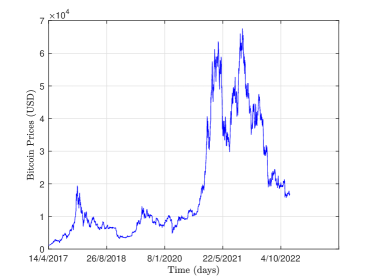
(a) Bitcoin prices

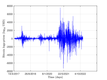
(b) Bitcoin log-prices

(c) Ethereum prices

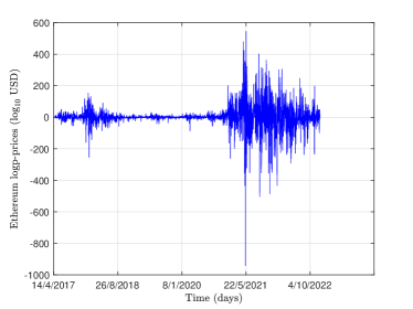
(d) Ethereum log-prices

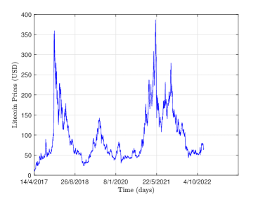
(e) Litecoin prices

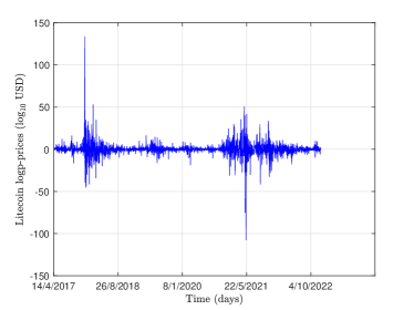
(f) Litecoin log-prices

Figure 1: Price and log-price time series of Bitcoin, Ethereum and Litecoin cryptocurrencies. The samples cover a daily period ranging from April 14, 2017, to December 22, 2022.

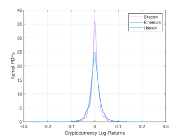
(a) Distributions

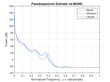
(b) Frequency spectra

Figure 2: Distributions of densities and frequencies (MUSIC: multiple signal classification) for the three cryptocurrency prices.

Table 1: Statistics and tests. Estimates with asterisks are performed on the returns (difference time series), while the remaining ones are obtained form level data.

Statistics		Bitcoin		Ethereum		Litecoin
Frequency		daily		daily		daily
Minimum		1176.8		48.50		10.21
Maximum		67527.9		4808.38		386.82
Mean		18423		1039.11		95.53
Std deviation		16759		1160.89		63.04
Coef. variation		90.97%		111.72%		66.00%
Kurtosis∗		13.7444		23.2517		60.7950
Skewness∗		-0.1825		-1.0370		0.9796
JB test∗		10006.1		35883.3		289543
ADF test∗		-47.1051		-49.3239		-47.3131
GPH∗ ($\hat{d}$)		0.14261		0.10744		-0.1173
BDS test∗		12.0452		15.6776		15.6328

Table 2: Distribution of outliers and extreme values.

Statistics		Bitcoin		Ethereum		Litecoin
$\sharp$ Low outliers		0		0		0
$\sharp$ High outliers		15		90		38
$\sharp$ Low extremes		0		0		0
$\sharp$ High extremes		0		0		1

Table 3: Summary statistics and long memory estimates of each cryptocurrency over the sub-intervals separated by change-points. Estimates with asterisks are performed on the returns (difference time series).

		Bitcoin		Ethereum		Liitecoin
Period 1		14 Apr 17 - 9 Oct 17		14 Apr 17 - 25 Nov 17		14 Apr 17 - 24 Nov 17
Mean		2903.45		250.490		45.134
Std dev.		1056.91		93.7091		16.555
IQR		1735.15		106.130		24.570
Hurst		0.22505		0.93235		0.45969
GPH∗ ($\hat{d}$)		-0.36109		0.23476		-0.12448
Period 2		10 Oct 17 - 11 Dec 19		26 Nov 17 - 13 Aug 18		25 Nov 17 - 29 Oct 18
Mean		7728.34		652.211		129.43
Std dev.		2908.34		226.730		68.709
IQR		3236.70		321.410		92.640
Hurst		0.62582		0.66038		0.61674
GPH∗ ($\hat{d}$)		0.06515		-0.14604		-0.16879
Period 3		12 Dec 19 - 5 Nov 20		14 Aug 18 - 25 Jul 20		30 Oct 18 - 18 Dec 20
Mean		9395.78		188.902		59.7041
Std dev.		1859.21		51.6290		23.4560
IQR		2508.85		80.6170		28.6850
Hurst		0.61835		0.52227		0.55140
GPH∗ ($\hat{d}$)		0.18060		-0.22222		0.08100
Period 4		6 Nov 20 - 13 Jun 22		26 Jul 20 - 3 Jan 21		19 Dec 20 - 24 Apr 22
Mean		42280.8		446.410		168.481
Std dev.		11748.4		105.901		51.1713
IQR		14677.7		145.810		61.0690
Hurst		0.57706		0.64929		0.29227
GPH∗ ($\hat{d}$)		-0.03314		0.10624		-0.17831
Period 5		14 Jun 22 - 22 Dec 22		4 Jan 21 - 26 May 22		25 Apr 22 - 22 Dec 22
Mean		19886.5		2808.45		62.1801
Std dev.		2176.17		885.903		12.2534
IQR		2377.25		1308.28		12.5731
Hurst		0.25147		0.54718		0.39737
GPH∗ ($\hat{d}$)		0.02084		0.02785		0.05454
Period 6		—		27 May 21 - 22 Dec 22		—
Mean		—		1422.94		—
Std dev.		—		239.391		—
IQR		—		384.142		—
Hurst		—		0.62192		—
GPH∗ ($\hat{d}$)		—		0.22322		—

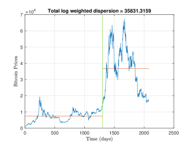
(a) Bitcoin: One change-point

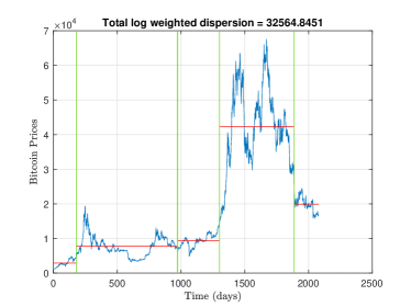
(b) Bitcoin: Four change-points

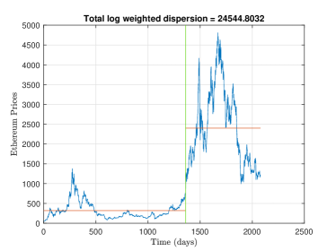
(c) Ethereum: One change-point

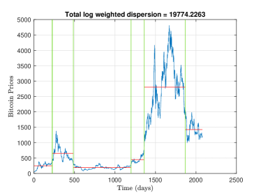
(d) Ethereum: Five change-points

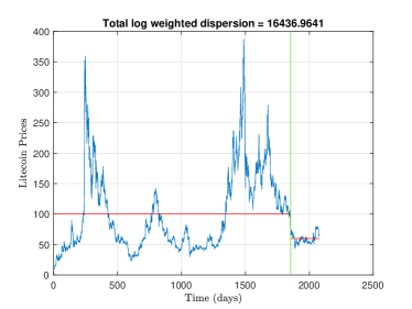
(e) Litecoin: One change-point

(f) Litecoin: Four change-points

Figure 3: Dividing the sampled period of the cryptocurrencies into a number of intervals using a test for multiple change-point detection (Left: the most significant change-point. Right: several change-points).

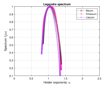
(a) Multifractal spectra

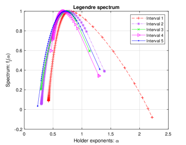
(b) Bitcoin’s structured multifractal spectrum

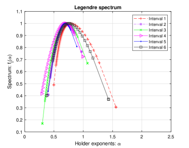
(c) Ethereum’s’s structured multifractal spectrum

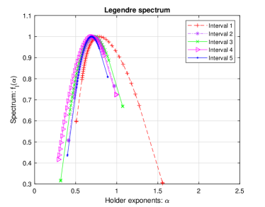
(d) Litecoin’s structured multifractal spectrum

Figure 4: Multifractality and structured multifractality of the three cryptocurrency prices.

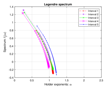
(a) Bitcoin shuffled data

(b) Bitcoin surrogate data

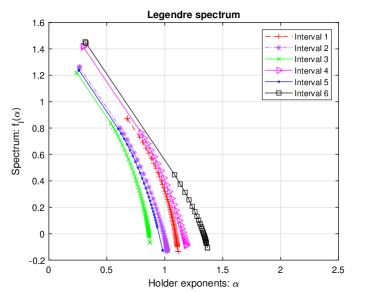
(c) Ethereum shuffled data

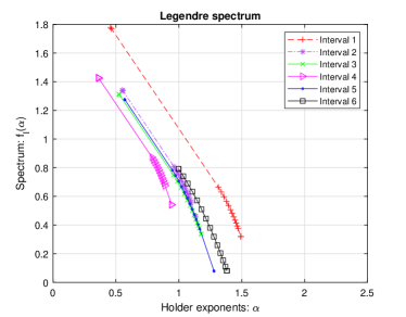
(d) Ethereum surrogate data

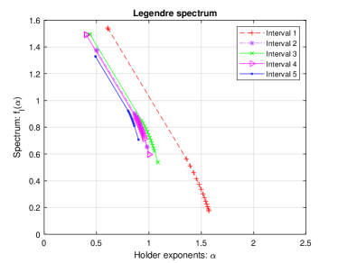
(e) Litecoin shuffled data

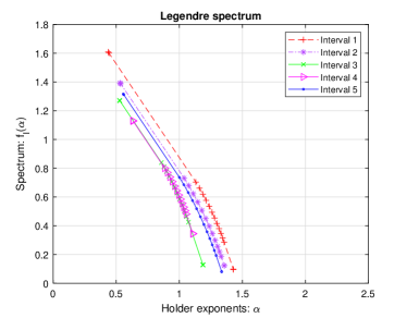
(f) Litecoin surrogate data

Figure 5: Reassessing structured multifractal scaling on shuffled and surrogate cryptocurrency time series.

After the three time series are split into adjacent intervals, a local MF-DFA is performed to each subsample. The objective is to test structural multifractality over this tense period in the history of the world economy. We are particularly interested in knowing whether the efficiency of the three major cryptocurrencies has changed significantly since the dates of the structural breaks. To address these issues, the approach defined in section 3 for testing structural multifractality is applied to the three prices. Noteworthy that Fraclab software [16] or the Matlab’s codes published by Ihlen [21] can be used at this stage. The first multifractal spectra to be interpreted in this section are those relating to the actual data, i.e., before splitting the time series (Figure 4(a)). The most surprising in these results is that the three cryptocurrencies have almost the same level of multifractality because the extent of the base of the arcs representing the spectra are almost equal. This is in addition to the other points of resemblance underlined above, such as the distributions of the log-returns, the frequency spectra as well as the number of extreme values (Figure 2). It is now important to show the points of dissimilarity between the three assets since this is the question that most interests investors, allowing them to explore alternative investment opportunities.

In Figure 4, the local Legendre spectra show that for the three cryptocurrencies, the local multifractality varies significantly from one sub-period to another. This confirms the basic hypothesis that multifractality is structural in nature, especially in periods of successive crises. The first interval including in particular the second and third quarters of 2017 seems to be the one where the multifractal scaling was the highest for the three cryptocurrencies. It is also important to note that the period of the COVID-19 outbreak characterized by record price levels had seen the reshrinking of multifractality levels for the three assets. It is as if the market tends to become less inefficient in times of high risk. We finish this visual analysis by applying the structural multifractality test on the shuffled and surrogate data in order to verify if this multifractality of these financial assets is to some degree related to self-dependence, distribution, or an underlying nonlinear correlation. Indeed, shuffling the raw series destroys the correlations in original series and keeps the distribution of original series, while generated surrogate series has a Gaussian distribution and the same linear correlations as the original series [56]. The spectra re-estimation results for each cryptocurrency are plotted in Figure 5. We can clearly see that the shapes reflecting multifractality become less obvious. This proves that the short-term dependencies, the distribution as well as the nonlinear autocorrelations are factors contributing significantly to this local multifractality.

3.3 Prediction Experiments

We finish our experiments in this paper with prediction tests applied to the three cryptocurrencies on each of the periods fixed above. In particular, we compare two types of fractional differentiation preceding learning using a neural network of the backpropagation category. This methodology remains one of the most widely used for forecasting and decision-making [51]. The objective is to compare the efficiency of a structured fractional modeling with that of a simple fractional modeling in a pure machine learning framework. For the first case, the fractional differentiation parameters by intervals are as estimated using the GPH method in Table 3. As for the overall differentiation, this is done based on the single parameter given in Table 1, also according to the GPH’s methodology. Noteworthy that Velasco’s [54] fractional differentiation technique and Shimotsu’s Matlab code are used in this step. The results of the predictions are summarized in Table 4. The mean absolute percentage error (MAPE) is used to express the prediction accuracy as a ratio defined by the formula:

$${\displaystyle{\mbox{MAPE}}={\frac{1}{n}}\sum_{t=1}^{n}\left|{\frac{A_{t}-F_{t}}{A_{t}}}\right|\times 100\%},$$ (21)

where $A_{t}$ is the actual value and $F_{t}$ is the forecast value. The results of the errors of this prediction phase are reported in Table 4. The predictions made here are complete reconstructions of the series of the three prices on each of the sub-periods all based on a Neural Autoregressive (NAR) model with 20 hidden layers, with sigmoid type activations and $p=5$ no lags. A Levenberg-Marquardt algorithm is used to train this neural network. We can note a relative improvement in the accuracy of predictions when differentiations are adapted to breakpoints occurring, which confirms that the locally multifractal time series require local transformations in order to obtain better performance from autoregressive models. In Figure 6, as a graphical illustration, we plot the predictions made by the NAR model based on the multi-fractional integration over the last three time periods. It is clear that the predictions reach an acceptable level of accuracy. It is now important to extend this type of neural model to equip it with a causal decision-making loop allowing it to also integrate other endogenous factors [42].

Table 4: Summary statistics and long memory estimates of each cryptocurrency over the sub-intervals separated by change-points. Estimates with asterisks are performed on the returns (difference time series).

	Method		Bitcoin		Ethereum		Liitecoin
Period 1
	FD-NAR		237.20		268.55		282.64
	LFD-NAR		234.45		241.32		281.01
Period 2
	FD-NAR		337.42		296.97		278.35
	LFD-NAR		145.40		279.44		222.78
Period 3
	FD-NAR		189.19		416.85		374.47
	LFD-NAR		180.22		254.09		223.97
Period 4
	FD-NAR		288.19		423.44		255.81
	LFD-NAR		284.88		377.17		242.65
Period 5
	FD-NAR		303.74		200.38		191.34
	LFD-NAR		192.33		195.34		182.34
Period 6
	FD-NAR		–		393.89		–
	LFD-NAR		–		277.56		–

(a) Bitcoin: Period 1

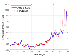
(b) Ethereum: Period 1

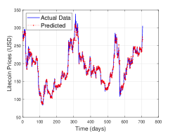
(c) Litecoin: Period 1

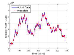
(d) Bitcoin: Period 2

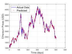
(e) Ethereum: Period 2

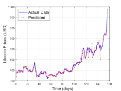
(f) Litecoin: Period 2

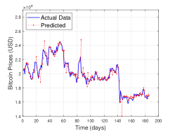
(g) Bitcoin: Period 3

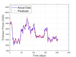
(h) Ethereum: Period 3

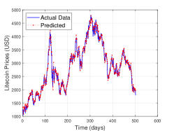
(i) Litecoin: Period 3

Figure 6: Prediction results of the three cryptocurrency prices over the last three intervals (see Table 3).

This study offered a new framework for multifractal data analytics, using a data mining methodology. The structural character of price fluctuation scaling could provide a basis for founding a new family of financial market forecasting models allowing decision makers to better anticipate future returns in situations of alternating economic and investment conditions between adverse and favorable. In particular, the new models could better identify time series characteristics such as trend, seasonality, and volatility, which can be particularly useful for companies that use time series to plan and assess financial performance. It is important to note that multifractal models are still relatively new and little used in the practice of finance. The results of these models are often dependent on the assumptions and data used, so they may not always be reliable for decision making. It is therefore important to use them in combination with other methods and to be aware of their limitations. It would also be interesting to extend the break detection methodology of our approach by adapting instead a more sophisticated method like that of the filtered derivative or the filtered derivative at p-value [10, 15], which generally assigns less importance to fake financial bubbles.

4 Conclusion

In this paper; we have defined a new notion of so-called structural multifractality allowing us to generalize the conventional principle of scaling. We have also developed an algorithmic approach to test this generalized multifractal character for a given time series. The main requirements of this approach is that it must be conducted on data sets of sufficient size, which makes it particularly suitable for big data. We then performed this on daily data from the three major cryptocurrencies over a significant period in the history of the global economy. This very particular global situation has made the irregularity of the fluctuations of these financial assets stronger than usual, which was moreover expected given the succession of important events such as Brexit, COVID-19 and the Russian-Ukrainian conflict. It was therefore essential to extend the principle of conventional multifractality towards a more general aspect in order to give more flexibility to the various econometric models intended for forecasting. The mechanism for measuring structural multifractal scaling essentially relies on a test for detecting structural changes on the studied time series, before an MF-DFA is performed on each of the resulting fluctuation regimes.

Visualizing the statistical results for the three cryptocurrencies allows us to confirm the basic hypothesis that the returns of these cryptocurrencies behave similarly to a structural multifractal process rather than a simple multifractal process. It seems, in fact, that the multiple breakpoints detected for each of the time series, sometimes coinciding with the major events of the period. These also seem to have an impact on the fluctuation dynamics, and therefore on the efficiency of the decentralized money market. Faced with this intermittent multifractal behavior, investors must equip themselves with an adaptive decision strategy, evolving with the fluctuating regime of the economic situation. In other words, any occurrence of a significant event on the economic scene must be a sign for investors of a change in the valuation of financial assets. New explainable machine learning forecasting models taking into account this generalized multifractality are therefore developed and tested on the different cryptocurrency prices.

In future research, it would be important to try understanding whether exogenous factors could also have contributed to this structural multifractality. The development and application of a structural multifractal cross-correlation analysis including other factors such as energy prices, the main stock market indices, or monetary exchange rates, can for example be a step in this direction. Multifractal cross-correlation of cryptocurrencies each other would also be relevant since it allows to locate the intervals of alternative investment opportunities. Finally, it would also be interesting to conduct forecasting experiments by designing intermittent multifractal autoregressive models as well. Such models could be implemented in massively parallel environments and tested on several types of economic and financial data, such as stock markets, electricity prices, oil prices, food prices, etc. All these perspectives can be realized in a politico-economic environment which remains tense with the continuation of the Russian-Ukrainian war.

Author statements

Ethical approval

Not required because the study did not touch on ethical issues requiring individual consent.

Competing interests

The authors declare no conflicts of interest.

Data availability statement

Data available on request from the authors.

References

- [1] Abry, P., Flandrin, P., Taqqu, M.S., and Veitch, D., (2003). Self-similarity and long-range dependence through the wavelet lens, Theory and Applications of Long-Range Dependence, Birkhäuser, pp. 527–556.
- [2] Aslam, F., Mohti, W., and Ferreira, P., (2020). Evidence of intraday multifractality in European stock markets during the recent coronavirus (COVID-19) outbreak, International Journal of Financial Studies, Volume 8, Issue 2, 31.
- [3] Aslam, F., Aziz, S., Nguyen, D.K., Mughal, K.S., and Khan, M., (2020). On the efficiency of foreign exchange markets in times of the COVID-19 pandemic, Technological Forecasting and Social Change, Volume 161, 120261.
- [4] Aslam, F., Ferreira, P., Ali, H., and Kauser, S., (2021). Herding behavior during the Covid-19 pandemic: a comparison between Asian and European stock markets based on intraday multifractality, Eurasian Economic Review, https://doi.org/10.1007/s40822-021-00191-4.
- [5] Aslam, F., Nogueiro, F., Brasil, M., Ferreira, P., Mughal, K.S., Bashir, B., and Latif, S., (2021). The footprints of COVID-19 on Central Eastern European stock markets: an intraday analysis, Post-Communist Economies, Volume 33, Issue 6, pp. 751–769.
- [6] Assaf, A., Bhandari, A., Charif, H., and Demir, E., (2022). Multivariate long memory structure in the cryptocurrency market: The impact of COVID-19, International Review of Financial Analysis, Volume 82, 102132.
- [7] Assaf, A., Mokni, K., Yousaf, I., and Bhandari, A., (2023). Long memory in the high frequency cryptocurrency markets using fractal connectivity analysis: The impact of COVID-19, Research in International Business and Finance, Volume 64, 101821.
- [8] Ben Ameur, H., and Louhichi, W., (2022). The Brexit impact on European market co-movements, Annals of Operations Research, Volume 313, pp. 1387–1403.
- [9] Ben Mabrouk, A., (2008). A higher order multifractal formalism, Statistics and Probability Letters, Volume 78, Issue 12, pp. 1412–1421.
- [10] Bertrand, P.R., Fhima, M., and Guillin, A., (2011). Off-line detection of multiple change points by the filtered derivative with p-value method, Sequential Analysis, Volume 30, Issue 2, pp. 172–207.
- [11] Bertrand, P.R., Fhima, M., and Guillin, A., (2013). Local estimation of the Hurst index of multifractional Brownian motion by increment ratio statistic method, ESAIM: Probability and Statistics, Volume 17, Issue ESAIM: PS, pp. 307–327.
- [12] Bouteska, A., Hajek, P., Fisher, B., and Abedin, M.Z., (2023). Nonlinearity in forecasting energy commodity prices: Evidence from a focused time-delayed neural network, Research in International Business and Finance, Volume 64, 101863.
- [13] Cao, G., Cao, J., and Xu, L., (2013). Asymmetric multifractal scaling behavior in the Chinese stock market: Based on asymmetric MF-DFA, Physica A: Statistical Mechanics and its Applications, Volume 392, Issue 4, pp. 797–807.
- [14] Catania, L., Grassi, S., and Ravazzolo, F., (2019). Forecasting cryptocurrencies under model and parameter instability, International Journal of Forecasting, Volume 35, Issue 2, pp. 485–501.
- [15] Elmi, M., (2014). Detection of multiple change points by the filtered derivative and false discovery rate, International Journal of Statistics and Probability, Volume 3, Issue 1, pp. 12–23.
- [16] Fraclab, (2017). FRACLAB, A fractal analysis toolbox for signal and image processing, INRIA 1998–2017, https://project.inria.fr/fraclab/.
- [17] Ftiti, Z., Louhichi, W., and Ben Ameur, H., (2021). Cryptocurrency volatility forecasting: What can we learn from the first wave of the COVID-19 outbreak?, Annals of Operations Research, https://doi.org/10.1007/s10479-021-04116-x.
- [18] Ghazani, M.M., and Khosravi, R., (2020). Multifractal detrended cross-correlation analysis on benchmark cryptocurrencies and crude oil prices, Physica A: Statistical Mechanics and its Applications, Volume 560, 125172.
- [19] Guo, H., Zhang, D., Liu, S., Wang, L., and Ding, Y., (2021). Bitcoin price forecasting: A perspective of underlying blockchain transactions, Decision Support Systems, Volume 151, 113650.
- [20] He, L-Y., and Chen, S-P., (2010). Are crude oil markets multifractal? Evidence from MF-DFA and MF-SSA perspectives, Physica A: Statistical Mechanics and its Applications, Volume 389, Issue 16, pp. 3218–3229.
- [21] Ihlen, E.A., (2012). Introduction to multifractal detrended fluctuation analysis in matlab, Frontiers in Physiology, Volume 3, pp. 141–159.
- [22] Kantelhardt, J.W., Zschiegner, S.A., Koscielny-Bunde, E., Havlin, S., Bunde, A., and Stanley, H.E., (2002). Multifractal detrended fluctuation analysis of nonstationary time series, Physica A Statistical Mechanics and Its Applications, Volume 316, Issues 1–4, pp. 87–114.
- [23] Killick, R., Fearnhead, P., and Eckley, I.A., (2012). Optimal detection of changepoints with a linear computational cost, Journal of the American Statistical Association, Volume 107, Issue 500, pp. 1590–1598.
- [24] Kamdem, J.S., Essomba, R.G., and Berinyuy, J.N., (2020). Deep learning models for forecasting and analyzing the implications of COVID-19 spread on some commodities markets volatilities, Chaos, Solitons and Fractals, Volume 140, 110215.
- [25] Kristjanpoller, W., and Bouri, E., (2019). Asymmetric multifractal cross-correlations between the main world currencies and the main cryptocurrencies, Physica A: Statistical Mechanics and its Applications, Volume 523, pp. 1057–1071.
- [26] Lahmiri,S., and Bekiros, S., (2021). The effect of COVID-19 on long memory in returns and volatility of cryptocurrency and stock markets, Chaos, Solitons and Fractals, Volume 151, 111221.
- [27] Lavielle, M., (2005). Using penalized contrasts for the change-point problem, Signal Processing, Volume 85, pp. 1501–1510.
- [28] Leigh, W., Purvis, R., and Ragusa, J.M., (2002). Forecasting the NYSE composite index with technical analysis, pattern recognizer, neural network, and genetic algorithm: a case study in romantic decision support, Decision Support Systems, Volume 32, Issue 4, pp. 361–377.
- [29] López-García, M.N., Trinidad-Segovia, J.E., Sánchez-Granero, M.A., and Pouchkarev, I., (2021). Extending the Fama and French model with a long term memory factor, European Journal of Operational Research, Volume 291, Issue 2, pp. 421–426.
- [30] Mandelbrot, B., (1967). The variation of some other speculative prices, The Journal of Business, Volume 40, Issue 4, pp. 393–413.
- [31] MathWorks, Inc. (2016). MATLAB, The language of technical computing. Natick, MA: The MathWorks. http://www.mathworks.com/.
- [32] Menéndez, P., Ghosh, S., and Beran, J., (2010). On rapid change points under long memory, Journal of Statistical Planning and Inference, Volume 140, Issue 11, pp. 3343–3354.
- [33] Mensi, W., Lee, Y-J., Al-Yahyaee, K.H., Sensoy, A., and Yoon, S-M., (2019). Intraday downward/upward multifractality and long memory in Bitcoin and Ethereum markets: An asymmetric multifractal detrended fluctuation analysis, Finance Research Letters, Volume 31, pp. 19–25.
- [34] Mensi, W., Sensoy, A., Vo, X.V., and Kang, S.H., (2022). Pricing efficiency and asymmetric multifractality of major asset classes before and during COVID-19 crisis, The North American Journal of Economics and Finance, Volume 62, 101773.
- [35] Mnif, E., Jarboui, A., and Mouakhar, K., (2020). How the cryptocurrency market has performed during COVID 19? A multifractal analysis, Finance Research Letters, Volume 36, 101647.
- [36] Naeem, M.A., Farid, S., Ferrer, R., and Shahzad, S.J.H., (2021). Comparative efficiency of green and conventional bonds pre- and during COVID-19: An asymmetric multifractal detrended fluctuation analysis, Energy Policy, Volume 153, 112285.
- [37] Norwood, B., and Killick, R., (2018). Long memory and changepoint models: a spectral classification procedure, Statistics and Computing, Volume 28, pp. 291–302.
- [38] Oh, H., and Thomas, R.J., (2010). Nonlinear time series analysis on the offer behaviors observed in an electricity market, Decision Support Systems, Volume 49, Issue 2, pp. 132–137.
- [39] Rabbouch, H., Saâdaoui, F., and Mraihi, R., (2017) Unsupervised video summarization using cluster analysis for automatic vehicles counting and recognizing, Neurocomputing, Volume 26, pp. 157–173.
- [40] Saâdaoui, F., (2010). Acceleration of the EM algorithm via extrapolation methods: review, comparison and new methods, Computational Statistics and Data Analysis, Volume 54, Issue 3, pp. 750–766.
- [41] Saâdaoui, F., (2012). A probabilistic clustering method for US interest rates analysis, Quantitative Finance, Volume 12, Issue 1, pp. 135–148.
- [42] Saâdaoui, F., & H. Rabbouch, (2014). A wavelet-based multiscale vector-ANN model to predict comovement of econophysical systems, Expert Systems with Applications, Vol. 41, No. 13, pp. 6017–6028.
- [43] Saâdaoui, F., Naifar, N., and Aldohaiman, M.S., (2017). Predictability and co-movement relationships between conventional and Islamic stock market indexes: A multiscale exploration using wavelets, Statistical Mechanics and its Applications, Volume 482, pp. 552–568.
- [44] Saâdaoui, F., (2018). Testing for multifractality of Islamic stock markets, Physica A: Statistical Mechanics and its Applications, Volume 496, pp. 263–273.
- [45] Saâdaoui, F., (2023). Skewed multifractal scaling of stock markets over the COVID-19 era, Chaos, Solitons and Fractals, Forthcomong.
- [46] Shao, Y.H., Xu, H., Liu, Y.L., and Xu, H.C., (2021). Multifractal behavior of cryptocurrencies before and during COVID-19, Fractals, Volume 29, Issue 6, id. 2150132.
- [47] Shrestha, K., (2021). Multifractal detrended fluctuation analysis of return on bitcoin, International Review of Finance, Volume 21, Issue 1, pp. 312–323.
- [48] Stosic, D., Stosic, D., Ludermir, T.B., and Stosic, T., (2019). Multifractal behavior of price and volume changes in the cryptocurrency market, Physica A: Statistical Mechanics and its Applications, Volume 520, pp. 54–61.
- [49] Takaishi, T., (2018). Statistical properties and multifractality of Bitcoin, Physica A: Statistical Mechanics and its Applications, Volume 506, pp. 507–519.
- [50] Takala, K., and Virén, M., (1996). Chaos and nonlinear dynamics in financial and nonfinancial time series: Evidence from Finland, European Journal of Operational Research, Volume 93, Issue 1, pp. 155–172.
- [51] Tang, W.H., and Röllin, A., (2021). Model identification for ARMA time series through convolutional neural networks, Decision Support Systems, Volume 146, 113544.
- [52] Telli, S., and Chen, H., (2020). Multifractal behavior in return and volatility series of Bitcoin and gold in comparison, Chaos, Solitons and Fractals, Volume 139, 109994.
- [53] Telli, S., and Chen, H., (2021). Multifractal behavior relationship between crypto markets and Wikipedia-Reddit online platforms, Chaos, Solitons and Fractals, Volume 152, 111331.
- [54] Velasco, C., (1999). Non-stationary log-periodogram regression, Journal of Econometrics, Volume 91, Issue 2, pp. 325–371.
- [55] Walasek, R., and Gajda, J., (2021). Fractional differentiation and its use in machine learning, International Journal of Advances in Engineering Sciences and Applied Mathematics, Volume 13, pp. 270–277.
- [56] Wu, L., Chen, L., Ding, Y., and Zhao, T., (2018). Testing for the source of multifractality in water level records, Physica A: Statistical Mechanics and its Applications, Volume 508, pp. 824–839.
- [57] Xu, N., Li, S., and Hui, X., (2021). Multifractal analysis of COVID-19’s impact on China’s stock market, Fractals, Volume 29, Issue 7, 2150.
- [58] Yi, E., Ahn, K., and Choi, M.Y., (2022). Cryptocurrency: Not far from equilibrium, Technological Forecasting and Social Change, Volume 177, 121424.
- [59] Yousaf, I., Patel, R., and Yarovaya, L., (2022). The reaction of G20+ stock markets to the Russia-Ukraine conflict ”black-swan” event: Evidence from event study approach, Journal of Behavioral and Experimental Finance, Volume 35, 100723.
- [60] Yolcu, U., Egrioglu, E., and Aladag, C.E., (2013). A new linear & nonlinear artificial neural network model for time series forecasting, Decision Support Systems, Volume 54, Issue 3, pp. 1340–1347.
- [61] Zhang, X., Yang, L., and Zhu, Y., (2019). Analysis of multifractal characterization of Bitcoin market based on multifractal detrended fluctuation analysis, Physica A: Statistical Mechanics and its Applications, Volume 523, pp. 973–983.