First Detection of the BAO Signal from Early DESI Data

Abstract

We present the first detection of the baryon acoustic oscillations (BAO) signal obtained using unblinded data collected during the initial two months of operations of the Stage-IV ground-based Dark Energy Spectroscopic Instrument (DESI). From a selected sample of $261,291$ Luminous Red Galaxies spanning the redshift interval $0.4<z<1.1$ and covering $1651$ square degrees with a $57.9\%$ completeness level, we report a $\sim 5\sigma$ level BAO detection and the measurement of the BAO location at a precision of $1.7\%$. Using a Bright Galaxy Sample of $109,523$ galaxies in the redshift range $0.1<z<0.5$, over $3677$ square degrees with a $50.0\%$ completeness, we also detect the BAO feature at $\sim 3\sigma$ significance with a $2.6\%$ precision. These first BAO measurements represent an important milestone, acting as a quality control on the optimal performance of the complex robotically-actuated, fiber-fed DESI spectrograph, as well as an early validation of the DESI spectroscopic pipeline and data management system. Based on these first promising results, we forecast that DESI is on target to achieve a high-significance BAO detection at sub-percent precision with the completed 5-year survey data, meeting the top-level science requirements on BAO measurements. This exquisite level of precision will set new standards in cosmology and confirm DESI as the most competitive BAO experiment for the remainder of this decade.

1 Introduction

The precise measurement of the expansion history of the Universe remains one of the key challenges in modern cosmology, and represents a compelling probe of the nature of dark energy (DE). The distance-redshift relation over a wide redshift range tests whether the accelerated expansion is consistent with a cosmological constant ($\Lambda$) or requires a dynamical explanation. It is also an important constraint on the growth rate of structures, allowing precise probes of gravity on cosmological scales, and on the Hubble constant, shedding light on the source of the “Hubble tension” as coming either from as-yet unappreciated astrophysical systematics or new physics. Finally, it breaks cosmological parameter degeneracies in, e.g., neutrino mass measurements. Recent results from state-of-the-art experiments have provided highly accurate constraints on the basic parameters of the standard spatially flat $\Lambda$CDM cosmological model, dominated by collisionless cold dark matter (CDM) and a DE component in the form of $\Lambda$ (Planck Collaboration et al., 2020; eBOSS Collaboration et al., 2021; Dark Energy Survey Collaboration et al., 2022).

The baryon acoustic oscillation (BAO) method is one of the most mature and robust probes of expansion history. Acoustic oscillations in the early pre-recombination Universe imprint a feature in the galaxy distribution at a scale ($r_{\rm d}$) set by the sound horizon evaluated at the drag epoch. The physics of these oscillations and the scale of this feature (which constitutes a fundamental standard ruler) are exquisitely calibrated by cosmic microwave background (CMB) measurements. Furthermore, the scale of the sound horizon is much bigger than the scale of physics of nonlinear structure formation and galaxy biasing, making it robust to the subsequent evolution of the Universe; for a review on BAO, see Weinberg et al. (2013) and references therein. The apparent size of this standard ruler across and along the line of sight characterizes the angular diameter distance ($D_{\rm A}$) and the Hubble parameter ($H$) as a function of redshift. Previous surveys have successfully measured these quantities directly from the BAO feature at different redshifts. Examples of first BAO detections obtained from multiple tracers include Eisenstein et al. (2005), Cole et al. (2005), Blake et al. (2012), du Mas des Bourboux et al. (2020), while the most recent results are reported in eBOSS Collaboration et al. (2021) and in Dark Energy Survey Collaboration et al. (2022).

BAO measurements at sub-percent precision are considered primary science targets for the Dark Energy Spectroscopic Instrument (DESI; DESI Collaboration et al., 2016), along with novel constraints on theories of modified gravity and inflation, and on neutrino masses. DESI, the only Stage-IV DE experiment that is currently taking data, aims to provide multiple sub-percent distance measurements over a broad $0<z<3.5$ redshift range. DESI represents an order-of-magnitude improvement both in the volume surveyed and in the number of galaxies measured over previous experiments – e.g., Extended Baryon Oscillation Spectroscopic Survey (eBOSS; Dawson et al., 2016), a key component of the fourth generation (SDSS-IV; Blanton et al., 2017) of the Sloan Digital Sky Survey (SDSS; York et al., 2000). In addition, DESI builds in a number of internal systematics checks using multiple tracer populations to probe common volumes.

Given the exquisite precision achievable by the DESI survey, the DESI collaboration decided to blind the redshift data to avoid any confirmation biases that can potentially impact all of the cosmological analyses. A general procedure to blind a modern redshift survey has been discussed in Brieden et al. (2020), and the exact implementation into the DESI framework will be described elsewhere. However, for early quality assurance tests and in order to validate the data processing and analysis pipelines, the first two months of DESI observations (hereafter referred to as DESI-M2) have been kept intentionally unblinded.

In this work, we use the DESI-M2 dataset and report the first high-significance detection of the BAO signal from the initial two months of DESI operations. As part of testing these early data, we integrate the eBOSS BAO pipeline into the DESI analysis framework, and apply such pipeline to measure the BAO scale with updates to accommodate all of the DESI specifics. While the DESI survey has four primary galaxy tracer populations to measure clustering, the survey strategy implies that not all tracers will have the same completeness in the very early data. The two most complete samples are the DESI Bright Galaxy Sample (BGS) and the Luminous Red Galaxies (LRGs). We focus on these two samples here for the BAO measurement, since our simulations suggest that we would not expect a BAO detection in the Emission Line Galaxy (ELG) and Quasar (QSO) samples given the number density, the low completeness, and the volume of this early data. A similar signal-to-noise (SN) consideration led us to concentrate on the isotropic distance measurements $\alpha\equiv D_{\rm A}^{2/3}H^{-1/3}/r_{\rm d}$, probed by the angle-averaged galaxy correlation function (the "monopole"). Future DESI analyses will present measurements using all four tracer populations, as well as measurements of $D_{\rm A}H$ from the Alcock-Paczynski effect (Alcock & Paczynski, 1979).

As we will show in our analysis, even these early data yield a precision in distance comparable to measurements from previously completed surveys (i.e., Anderson et al., 2012; Bautista et al., 2021), highlighting the remarkable statistical power of the DESI data. In the spirit of the DESI blinding policy, we restrict ourselves to providing just the statistical precision of the measurements rather than the actual distance values – which will be presented instead in a series of DESI Year 1 (Y1) forthcoming cosmological papers. This work therefore should be seen as an end-to-end quality assurance of the DESI data management system, as well as an early validation of the DESI spectroscopic pipeline.

The layout of the paper is organized as follows. In Section 2, we briefly describe the main aspects of the DESI-M2 sample used in this work, along with the procedure to build the corresponding large-scale structure (LSS) data catalogs. In Section 3, we present the approximate and $N$-body-based mocks adopted in the core analysis, and explain how such synthetic catalogs are constructed in order to mimic the complex footprint and characteristics of the DESI-M2. In Section 4, we illustrate all of the analysis tools, namely the chosen two-point clustering estimator, the density field reconstruction technique, and the BAO fitting methodology. Section 5 addresses covariance matrices, and in particular the construction, calibration, and validation on mock data of semi-analytical semi-empirical covariances for the BAO fitting procedure. More details on the covariance matrices adopted here are reported in a companion paper (Rashkovetskyi et al., 2023). The main results are detailed in Section 6, where we assess the precision and detection statistics of the BAO feature in the LRG and BGS samples. We then briefly address the expected precision of the final Year 5 (Y5) DESI LRG sample in Section 7, in terms of the BAO detection level, based on forecasts obtained from our promising early results. Finally, we conclude in Section 8, where we summarize the main findings and highlight the relevance for the upcoming Y1 DESI dataset. We also leave some additional material in Appendix A.

2 DESI Main Survey Data: First Two Months

In this section, we provide a concise description of the DESI-M2 dataset, along with several specifics on the LSS catalog construction. A number of additional technical details can be found in the quoted supporting papers, many of which are still in a preparatory phase and will be available at the time of the official Y1 DESI data release.

2.1 DESI Early Data: General Aspects

Table 1: Statistics of the four primary DESI targets from the DESI-M2 dataset, including completeness information.

Target	$N_{\rm North}$	$N_{\rm South}$	$N_{\rm Total}$	$z$ range	Area [deg2]	Completeness
BGS Bright	239492	390988	630480	0.1 - 0.5	3677	0.500
BGS Bright, $M_{r}<-21.5$	38472	71051	109523	0.1 - 0.5	3677	0.500
LRG	80651	180640	261291	0.4 -1.1	1651	0.579
ELG	55383	117145	172528	0.8 - 1.6	976	0.297
QSO	70337	153453	223790	0.8 - 3.5	2906	0.778

DESI began its main program on May 17, 2021. Its commissioning and ‘Survey Validation’ (SV) phases (DESI Collaboration et al., 2023a) had proved the instrument (Abareshi et al., 2022) and operations strategy (Schlafly et al., 2023) to be efficient. The DESI collaboration decided that the first two months of the observations of DESI main survey data (i.e., DESI-M2) could be analyzed without the blinding restrictions imposed on the rest of the sample that will be used for DESI Y1 Key Projects.

The DESI-M2 data were observed on nights in 2021 from May 14th through July 9th on 304 dark time and 342 bright time ‘tiles’. Each tile represents a specific sky location pointing of the telescope and specific target selection for each of the 5000 robotic positioners populating the DESI focal plane (Silber et al., 2022) determined by the DESI fiberassign software (Raichoor et al. in preparation). The spectra extracted from these observations were reduced by the DESI spectroscopic pipeline (Guy et al., 2023) and released to the DESI collaboration as the Guadalupe spectroscopic product. The redshift measurements in these Guadalupe data are used in this paper and will be made public with the DESI Y1 data release (DR1), i.e., they are not available in the DESI early data release (EDR; DESI Collaboration et al. 2023b).

The DESI-M2 tiles are primarily first pass tiles that do not overlap each other. In dark time, the full DESI survey observes tiles in 7 overlapping passes, with a median overlap of 5 (Schlafly et al., 2023). Thus, the DESI-M2 data are substantially less complete in the area observed than they will be when the survey is finished. This incompleteness affects all samples, but is most extreme for the target classes that are given the lowest priority during the assignment of fibers on a tile (DESI fiber assignment is reported in Raichoor et al. in preparation). We describe this further next, when discussing the different DESI target classes.

2.2 DESI Targets

DESI divides its observing time into a ‘bright’ and a ‘dark’ time program, for which the targeting is done independently (Myers et al., 2023). During dark time, in order of priority for fiber assignment, QSOs (Chaussidon et al., 2023), LRGs (Zhou et al., 2023), and ELGs (Raichoor et al., 2023) are observed. QSOs with redshifts greater than $2.1$ are selected for follow-up in order to increase the SN of the spectra in the Ly$\alpha$ forest region. During bright time, a BGS (Hahn et al., 2023) is observed, which has a ‘Bright’ and ‘Faint’ component, as well as Milky Way stars (MWS; Cooper et al. 2022). In this work, we only consider the higher priority BGS Bright sample.

For detailed discussions of how these target samples were chosen, we refer the reader to the individual selection papers previously cited. Table 1 summarizes key properties of the samples and Figure 1 shows the redshift distribution of each sample. Combined, they will allow measurements of large-scale clustering modes at better than the sample variance limit to $z<1.6$ (DESI Collaboration et al., 2023a). The QSO sample provides this information at a lower sampling rate all the way to redshifts greater than $3$ and further samples density fluctuations via the variance of Ly$\alpha$ forest absorption in each spectrum. The BGS sample is approximately flux limited and thus has a spatial density that rapidly increases as the redshift gets lower and is approximately sample variance limited to $z<0.5$. There is also substantial overlap between the LRG and ELG catalogs, which will allow comparison between results obtained from the most massive and passive galaxies (LRG) and those that are actively star forming (ELG).

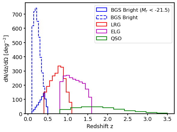
Figure 1: Redshift distribution of the four primary DESI tracers, from the DESI-M2 clustering catalogs.

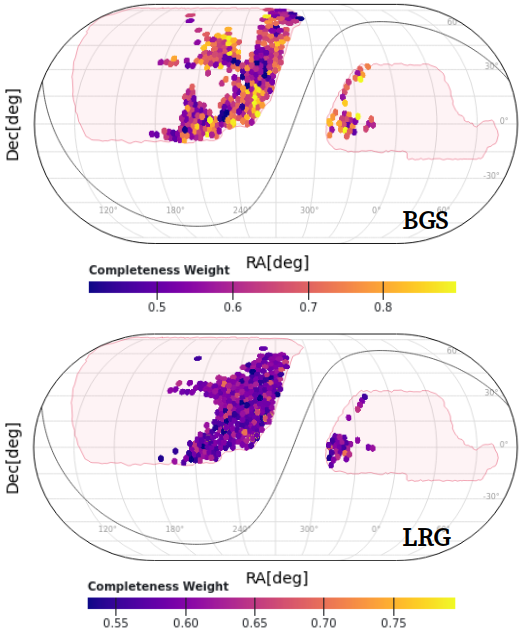
Figure 2: Footprints of the DESI-M2 BGS Bright (top) and LRG (bottom) clustering samples, color-coded by completeness weights. The total areas highlighted by the pink color represent the final DESI Y5 expected footprint. The specific DESI-M2 areas covered by the BGS Bright and LRG samples are respectively 3677 deg² and 1651 deg².

2.3 LSS Catalog Construction

The construction of the LSS catalogs involves determining the area on the sky where good observations were possible for each tracer, applying criteria on the DESI data to select reliable redshifts within a given redshift range, and providing weights that correct for variations in observing completeness, target density due to changes in imaging conditions, and relative redshift success due to variations in DESI observing. The overall process is similar to that applied to SDSS (most recently eBOSS; Ross et al. 2020), with the specific details of DESI observations accounted for as we describe here. The pipeline that was applied to the DESI-M2 sample represents an early version of the DESI LSS catalog pipeline, which will be fully described (and considerably improved) in Y1 publications. Many aspects of the pipeline match that applied to the DESI ‘One Percent Survey’, which is detailed in the overall description of the DESI EDR (DESI Collaboration et al., 2023b). In what follows, we provide details on the specific choices applied for DESI-M2.

The ‘randoms’ that populate the sky area where good observations were possible were produced using the same procedures as applied to the DESI One Percent Survey LSS catalogs. DESI randoms are produced using a standard such that each individual (and independent) set has a density of $2500$ deg^-2. We use $10$ such sets for the DESI-M2 clustering measurements and thus the total sky density of the random samples used is $25000$ deg^-2. The process of creating DESI randoms produces significantly different areas for different tracer types due to the priority masking (e.g., we have no randoms in areas where LRGs could not have been observed because a higher priority QSO target was assigned to the fiber positioner associated with that sky location). In order to determine the effective area occupied by each sample, we simply count the number of randoms in one of the final LSS random catalogs sets and divide by $2500$ deg^-2. These areas are given in Table 1. While the total effective area is considerably different per tracer, the footprint of tiles is the same for all dark/bright time tracers. Figure 2 shows the footprint of tiles for BGS (bright time; top panel) and LRG (dark time; bottom panel) tracers. The plot is constructed via a web interface provided by David Kirkby, and it is color coded by the completeness in each tile grouping.

For the data samples, we follow the same procedures as applied to the One Percent Survey LSS catalogs (described with the EDR) in order to select targets of the given type that could have been observed. Any unobserved targets at this stage were not observed because a target of the same type was instead observed at the given sky location. Each observed target is given a completeness weight, WEIGHT_COMP, equal to the total number of targets (of the given type) at the location of the observed target (with unique ‘locations’ determined by the combination observed tile and fiber positioner; see DESI Collaboration et al. 2023b for more details). In particular, we note that the fiber patrol radius is at most 89”: it depends on e.g., the focal plane position due to the optics.

The criteria for the BGS and LRG samples we focus this study on are:

• LRG: $0.4<z<1.1$, ZWARN$=$0, DELTACHI2$>$15

• BGS: $0.1<z<0.5$, ZWARN$=$0, DELTACHI2$>$40.

ZWARN is a bitmask generated by the redshift pipeline (Guy et al., 2023), where any non-zero value indicates a problem. The criteria on DELTACHI2, which is the difference in $\chi^{2}$ between the two best-fitting redshift solutions, were shown to provide pure and complete samples in the respective targeting papers (Hahn et al. 2023; Zhou et al. 2023). For LRGs, the choice of redshift range is motivated by the fact that the number density is approximately constant at $5\times 10^{-4}(h^{-1}{\rm Mpc})^{3}$ between $0.4<z<0.8$. At $z>0.8$, the LRG density decreases mostly due to the sample’s minimum flux threshold and is less than $1\times 10^{-4}(h^{-1}{\rm Mpc})^{3}$ for $z>1.1$. Similarly, the density of the BGS sample decreases to less than $1\times 10^{-4}(h^{-1}{\rm Mpc})^{3}$ for $z>0.5$. For the BGS sample, we also apply an absolute magnitude cut in the $r$-band $M_{\rm r}<-21.5$. When obtaining the absolute magnitude, we simply apply the distance modulus, i.e., we do not apply any corrections for evolution (‘e’ correction) or the shape of the spectrum (‘k’ correction). The cut provides a sample with roughly constant number density at $\sim 8\times 10^{-4}h^{3}$Mpc^-3 and clustering amplitude for $z<0.4$ and is thus sufficient for our preliminary study. Future DESI studies will likely include k+e corrections, especially for the selection of BGS samples.

We then add two more weights in order to account for variations in the selection of the data. The first corrects for fluctuations in the target data that are due to variation in the imaging data quality. To do so, we apply the random forest regression method (Chaussidon et al., 2021) available as an option in the regressis package, given maps of imaging properties compiled by the DESI targeting team. The data (after redshift cuts) and randoms are combined to produce a map of the projected density of the sample at Healpix (Górski et al., 2005) $N_{\rm side}=256$ and is compared to maps of the depth and PSF size in the $g$, $r$, $z$, and $W1$ bands, the $E(B-V)$ Galactic extinction according the Schlegel et al. (1998) dust maps, and the stellar density observed in the Gaia 2nd data release (Gaia Collaboration et al., 2018). The regressis random forest method is used to determine a model of the projected density fluctuations as a function of those map quantities and the inverse of the model is included in the catalogs as a weight, ‘WEIGHT_SYS’. For our LRG and BGS samples, very similar clustering results are obtained when instead obtaining the weights using the linear regression method applied to eBOSS, described in (Ross et al., 2020).

After, we obtain a weight to account for variations in redshift success based on the particulars of DESI observations. Zhou et al. (2023) showed that the LRG redshift success can be modeled as a function of the effective observing time and the target’s fiber flux in the $z$-band. A similar dependency exists for BGS, with the $r$-band fiber flux the relevant photometric quantity. The inverse of the best-fit model for the failure rate is used as ‘WEIGHT_ZFAIL’. We find that applying these redshift failure weights has very little impact on the clustering measurements used in this work.

Next, we determine ‘FKP’ weights (Feldman et al., 1994) in order to properly weight each volume element with respect to how each sample’s number density changes with redshift. This is simply given by:

$$w_{\rm FKP}=\frac{1}{1+n(z)CP_{0}}$$ (1)

where $n(z)$ is the weighted number per volume, $C$ is the mean completeness for the sample, and $P_{0}$ is a fiducial power-spectrum amplitude. We use $P_{0}=10^{4}(h^{-1}{\rm Mpc})^{3}$ for LRGs and $P_{0}=7\times 10^{3}(h^{-1}{\rm Mpc})^{3}$ for BGS. These values approximately match the monopole of the power spectrum at $k=0.15h/{\rm Mpc}$ for the respective samples.

The redshifts and all four weights are then randomly sampled from the data catalog and attached to the random catalogs in order to match the radial selection function. Finally, the catalogs are normalized separately (and all weights are fit for separately) in the North and South photometric regions.

3 Mock Catalogs

In our analysis, we utilize DESI mock galaxy catalogs for statistically testing the performance of the BAO fits, as well as for validating the adopted covariance matrices in terms of BAO fitting. Here, we briefly describe the main characteristics of the various sets of mocks, along with the DESI customization procedure to include survey realism.

3.1 DESI Mocks: General Description

We use two different sets of DESI mock galaxy catalogs for the LRG sample: one type is directly constructed from $N$-body simulations (i.e., AbacusSummit; Maksimova et al., 2021), while a second type is based on approximated methods (i.e., EZmocks; Zhao et al., 2021).

The $N$-body-based realizations are part of the first official set of DESI mock galaxy catalogs (Alam et al. in preparation) which were calibrated based on an early reduction of the One Percent Survey spectroscopic data for LRG (see Section 3.3). This set is made of $25$ cutsky simulations based on the $2\,h^{-1}{\rm Gpc}$ AbacusSummit runs. The halo occupation distribution (HOD) model for LRGs is calibrated using small-scale (below $5\,h^{-1}{\rm Mpc}$) wedges in combination with large-scale bias evolution where available. The LRG mocks are further subsampled to approximately match the $n(z)$ distribution of the specific LRG sample (called ‘main’) considered in this paper (see Figure 16 of Zhou et al., 2023, for the ‘main’ selection in the One Percent Survey). The mocks implementing the DESI survey geometry and specifics (denoted as ‘cutsky’ mocks) are generated using the simulation output near the primary redshift of LRGs that we do not report in this paper. The $2\,h^{-1}{\rm Gpc}$ box is repeated and then the coordinates are converted to sky coordinates.

The approximate mock realizations consist of 1000 EZmocks for LRGs, and are built with an elaborated procedure centered on the Zel’dovich approximation (Zel’dovich, 1970). They do account for stochastic scale-dependent, non-local, and nonlinear biasing contributions: extensive details on the production methodology can be found in the original release paper by Chuang et al. (2015). The EZmocks have accurate clustering properties consistent with the previously described $N$-body-based AbacusSummit realizations – and nearly indistinguishable from actual $N$-body solutions – in terms of one-point, two-point, and three-point statistics.

We note that we have decided not to use any mocks for the BGS sample, primarily for reasons related to a calibration performed with an earlier DESI dataset than the one considered in this study.

3.2 DESI Mocks: Masking and Customization

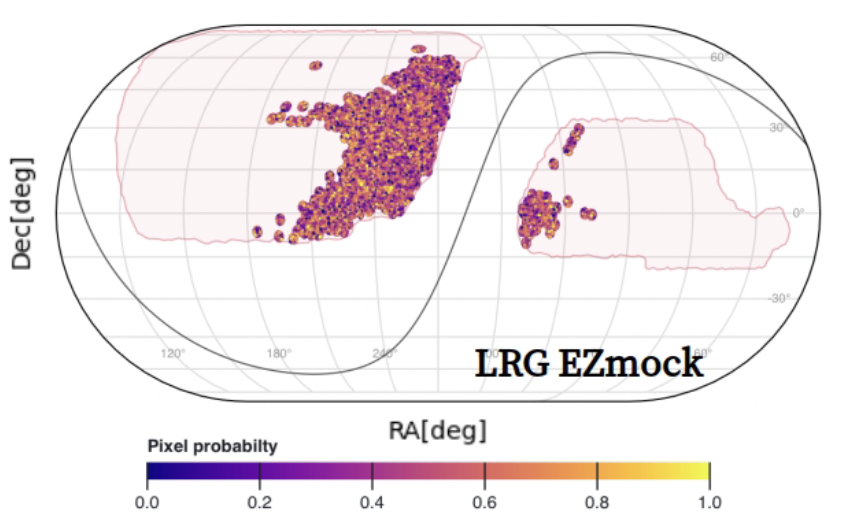
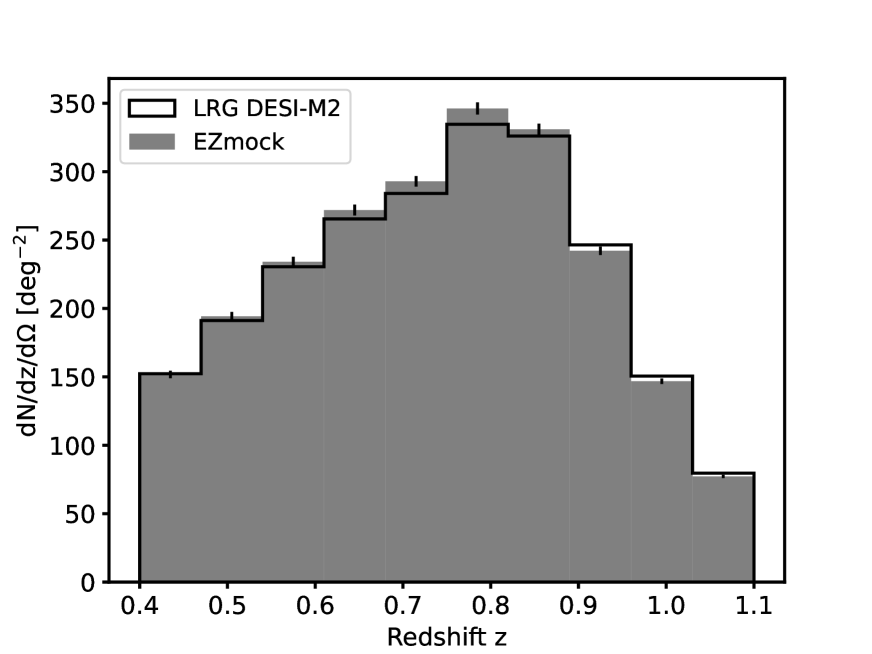
Figure 3: [Top] Map of a single LRG EZmock realization with the pixel probability of the HEALPix mask. [Bottom] Dispersion of $1000$ LRG EZmocks, after application of the different masks described in Section 3.2, compared with the actual LRG DESI-M2 redshift distribution.

An important step in the mock-making pipeline is the incorporation of survey realism, namely the characteristics of the various synthetic realizations need to accurately match the properties of the DESI-M2  sample. This is achieved via the application of a succession of masks, as we schematically describe in what follows.

Survey Masks. We subsample the mocks using a tile mask matching the footprint of DESI-M2 and match the redshift distribution of each target: for LRGs, the $n(z)$ distribution is based on DESI-M2 results (Figure 2), while for BGS on the One Percent Survey distribution. This tile mask cuts the data and random to the circular region around each tile center.

Intra-tile Geometry. The geometrical area where DESI targets could have been observed is obtained for the data catalogs following the procedure described in Section 2.3. In order to analyze all $1000$ mocks, we approximate the results of the procedure run on the data using a HEALPix (Górski et al., 2005) map built from the random catalogs. As a reference, we utilize the same random cuts to the target catalog sky area that were the inputs to the LSS catalog process, additionally cutting them to be within the tile area previously defined. In every $N_{\rm side}=1024$ pixel, we count the number of randoms in both the LSS catalog and in the reference randoms. The ratio of these counts approximates the small-scale holes in the observed footprint. We apply it by sub-sampling the mock data and randoms by the fraction in each pixel. In this way, the effective area of the footprint, as determined by summing random points assumed to have a constant surface density, matches that of the observed data. This is shown as an example in the top panel of Figure 3, to be compared with the bottom panel of Figure 2.

Incompleteness Assignment. At this stage, we still have more simulated galaxies than those observed in the actual DESI data. This is because, for most of the locations, only one fiber is available to observe multiple targets. In order to approximate this effect in terms of number counts, we simply take the overall assignment completeness of the data in the LSS catalogs, i.e., $N_{\rm observed}/N_{\rm total}$, where $N_{\rm total}$ is the number of targets within the DESI-M2 footprint where observations were possible. This type of completeness should vary strongly as a function of the number of overlapping DESI tiles, but we simply apply a constant factor (an average of $0.51$ for the $1000$ realizations) given that over $90\%$ of the DESI-M2 area is covered by only a single tile. To this end, the bottom panel of Figure 3 shows that the observed DESI-M2  LRG redshift counts per square degree match well those obtained from mock data, after applying the assignment incompleteness factor. This procedure is implemented in the $N$-body based AbacusSummit realization as well as in the approximate EZmocks. Finally, we note that the incompleteness will be modeled more rigorously for the forthcoming DESI Y1 analysis.

3.3 DESI Mocks: Calibration

In terms of clustering properties (see Section 4.1), the two sets of mocks described here have been tuned via survey and completeness masks with an earlier version of the DESI LRG clustering measurements (i.e., One Percent Survey data) having a 10% lower amplitude than the DESI-M2 LRG sample considered in the current study. This can be readily inferred from Figure 4, where we contrast the observed LRG clustering in the DESI-M2 sample at $r\sim 20\,h^{-1}{\rm Mpc}$ with the average clustering of 1000 LRG EZmocks. For this reason, in the present analysis mocks are only used for validation purposes, and we will be adopting semi-analytical semi-empirical covariances rather than mock-based covariances for our primary BAO fits – as described in Section 5. In fact, a calibration offset in the two-point clustering (although located outside of the BAO fitting range) would manifest in a substantial difference in the covariance between different scales, causing a 17.6% impact on the resulting BAO precision when pairing such a mock-based covariance matrix with the actual data clustering.

Figure 4: Monopole of the LRG two-point correlation function before reconstruction, as measured from the DESI-M2 sample (blue dots) and from the average of 1000 EZmocks (orange dots). Data errorbars are obtained from a jackknife covariance directly inferred from DESI-M2 LRGs, while mock errorbars are drawn from the LRG EZmock sample covariance. As mentioned in the main text (Section 3.3), the $\sim 10\%$ difference near the $\sim 20~{}\,h^{-1}{\rm Mpc}$ peak is not surprising, as these mocks were tuned with an earlier version of the DESI data. Hence, in the present work mocks are only used for validation purposes.

4 Analysis Methods

In this section, we illustrate all of the analysis tools adopted in our work, from the two-point clustering estimator to the density field reconstruction, until the BAO fitting methodology. In particular, the DESI team is currently studying all aspects of the BAO pipeline given the stringent requirements on theoretical and observational systematics that will be imposed by a dataset as powerful as we expect by the end of the survey. For the investigation of this preliminary DESI-M2 data, and to make contact with earlier work on the subject, we choose to largely follow the analysis choices made by the BOSS/eBOSS surveys. We highlight these choices in what follows, while referring the reader to the original papers for more extensive details.

4.1 Two-Point Correlation Function Estimator

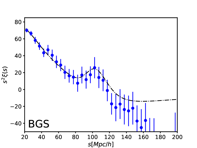
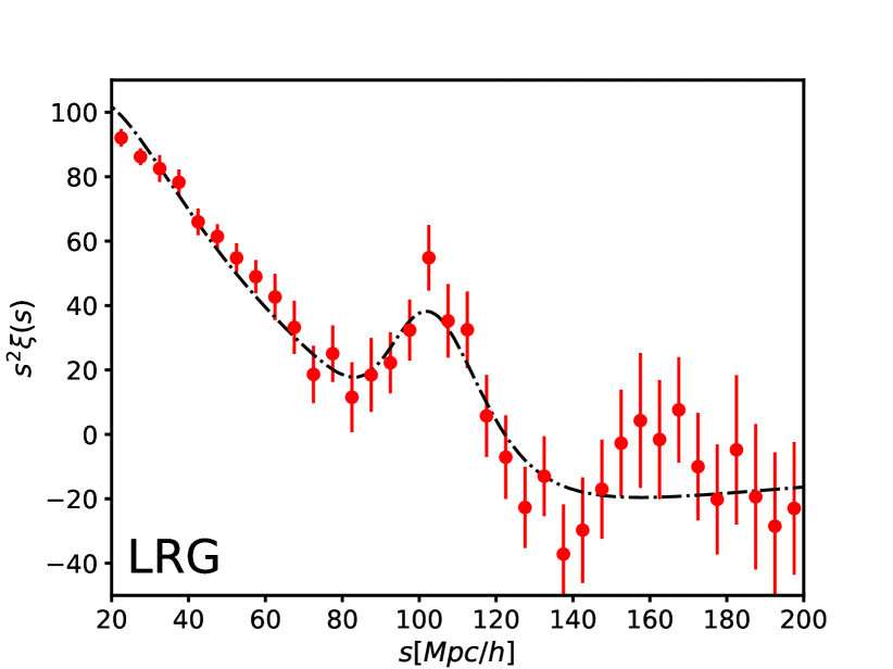
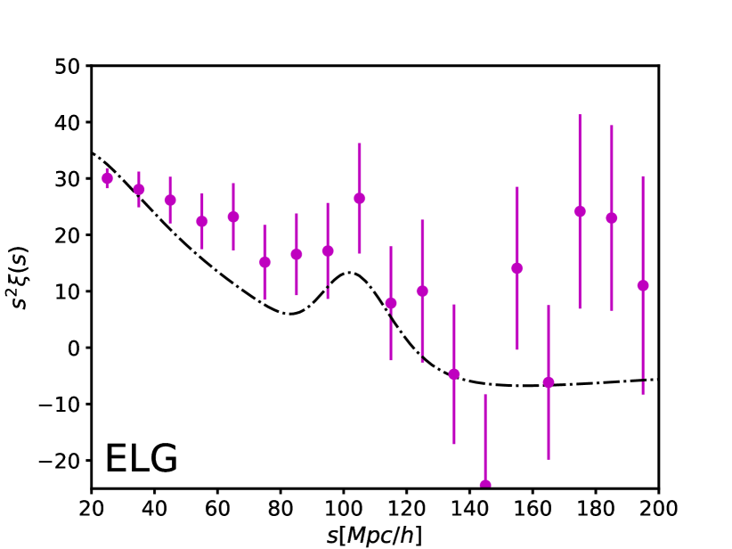
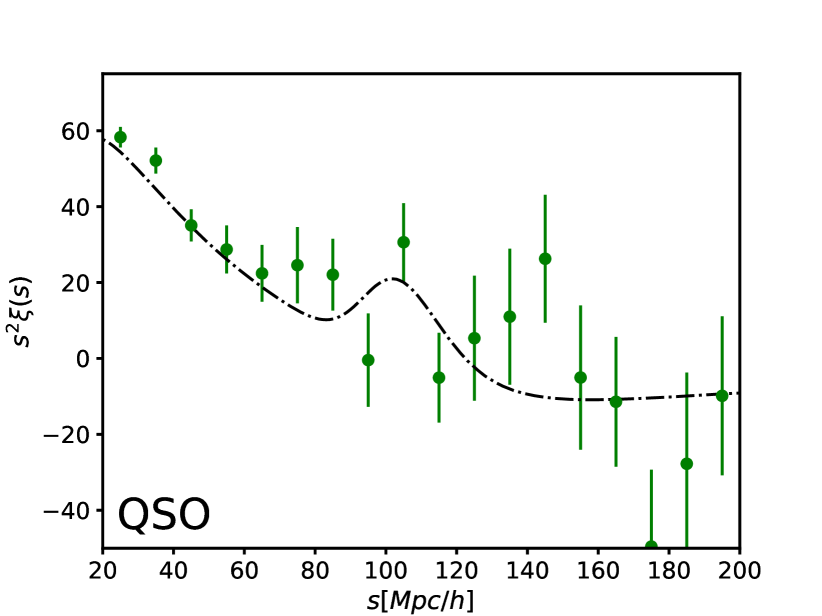
Figure 5: Two-point correlation function measurements of the four DESI tracers, obtained from the DESI-M2 sample. Errorbars are derived from the diagonal of the corresponding covariance matrixes, although we caution the reader of a significant bin-to-bin correlation in these measurements. Model curves are simple damped linear theory predictions that indicate the expected overall clustering amplitude and BAO damping typical at the mean redshift of the target samples.

We compute all of the anisotropic redshift-space correlation functions $\hat{\xi}$’s with the well-known Landy-Szalay estimator (LS; Landy & Szalay, 1993), namely:

$$\hat{\xi}(s,\mu)=\frac{DD(s,\mu)-2DR(s,\mu)+RR(s,\mu)}{RR(s,\mu)},$$ (2)

where $DD(s,\mu)$ and $RR(s,\mu)$ are the normalized weighted number of pairs in the data and random catalogs – respectively – binned as a function of the separation $s$ between two galaxies, $\mu\in[-1,1]$ is the cosine angle between the galaxy pair and the line of sight (LOS), and $DR(s,\mu)$ denotes pair counts between data ($D$) and randoms ($R$). The LS estimator gets modified when the reconstruction procedure (described in Section 4.2) is applied. In essence, a shifted random catalog (termed $S$) should be used in the numerator of Equation (2) in substitution of $R$, and one needs to replace $DR$ with $DS$ and $RR$ with $SS$, respectively. We use $200$ $\mu$-bins spanning the interval [$-1,1$] and $4h^{-1}{\rm Mpc}$ $s$-bins for BGS and LRGs.

The anisotropic correlation function $\hat{\xi}(s,\mu)$ is then integrated over the Legendre polynomials $\mathcal{L}_{\ell}(\mu)$ to obtain the various multipoles; in the current analysis, we only use the monopole, i.e., $\ell=0$:

$$\hat{\xi}_{\ell}(s) =\frac{2\ell+1}{2}\int_{-1}^{1}d\mu\hat{\xi}(s,\mu)\mathcal{L}_{\ell}(\mu)$$ (3)

$$\simeq\frac{2\ell+1}{2}\sum_{i}\hat{\xi}(s,\mu_{i})\int_{\Delta\mu_{i}}d\mu\mathcal{L}_{\ell}(\mu).$$ (4)

In the last equality, we have made explicit the discrete sum over $\mu$-bins, weighted by the analytic integral of $\mathcal{L}_{\ell}(\mu)$ over each $\mu$-bin having width $\Delta\mu_{i}$.

All of the two-point correlation function calculations are performed with the Python package pycorr, which wraps a modified version of the Corrfunc package (Sinha & Garrison, 2019, 2020).

Figure 5 shows the observed two-point correlation functions of the four tracers discussed in Section 2.2, contrasted with simple damped linear theory models that indicate the expected overall clustering amplitude and BAO damping typical at the mean redshift of the target samples. From LRGs and BGS, we observe a local bump near the expected location of the BAO peak. Moreover, while BGS observations appear to lie systematically below the model curve at scales greater than $120h^{-1}{\rm Mpc}$, this is simply because there are fewer modes at larger separations in these early DESI data. Therefore, they are highly correlated and thus the amplitude of the two-point correlation function decreases at those scales. For ELGs and QSOs, the amplitude of the observed clustering appears consistent with the theoretical expectations (within errors), although it is challenging to identify a clear BAO-like signature. Indeed, we do not expect a BAO detection from ELGs and QSOs of the DESI-M2 sample, given the small survey volume in combination with the low completeness (ELGs) and high shot noise (QSOs).

4.2 Density Field Reconstruction

We apply the density field reconstruction technique (Eisenstein et al., 2007) on the observed galaxy density fields in order to partially recover the BAO feature that has been degraded due to structure growth and redshift space distortions (RSD). To do so, we follow the iterative procedure described in Burden et al. (2015), as implemented in the IterativeFFTReconstruction algorithm of the pyrecon package with the RecIso convention. The density contrast field is smoothed by a Gaussian kernel of width $15\,h^{-1}{\rm Mpc}$ and three iterations are performed, assuming an approximate growth rate and the expected bias for each sample. The choice of these reconstruction conditions along with the assumed fiducial cosmology were shown to have a very marginal impact on BAO measurements in earlier galaxy survey samples – i.e., see Vargas-Magaña et al. (2018) and Carter et al. (2020).

4.3 BAO Fitting Methodology

Table 2: Covariance matrices utilized in this work.

Name	Tracer	Notes
DESI-M2-EZ	LRG	Constructed from EZmock clustering
RascalC-EZ	LRG	RascalC calibrated on EZmock clustering
RascalC-LRG	LRG	RascalC calibrated on DESI-M2 LRG clustering
RascalC-BGS	BGS	RascalC calibrated on DESI-M2 BGS clustering

We employ the same BAO fitting pipeline that has been previously applied to a large number of BOSS and eBOSS analyses (Ross et al., 2017; Ata et al., 2018; Hou et al., 2020; Raichoor et al., 2020). The accuracy of such methodology was demonstrated to be sufficient at the precision demanded by BOSS/eBOSS data, especially for determining the isotropic BAO scale. However, advances are expected to be necessary in order to meet the exquisite precision expected for DESI Y5, and thus an improved DESI pipeline is currently under development and will be presented along with the DESI Y1 analyses.

In this study, we only fit for the monopole of the correlation function, hence for the isotropic scaling parameter $\alpha$. Our BAO pipeline is ‘template-based’, and it essentially coincides with the algorithm introduced by Xu et al. (2012). However, the BAO templates are generated via the formulae defined by Equations 9-13 of Ross et al. (2017), where the linear power spectrum is split into a BAO and a no-BAO components, and damping is added solely to the BAO that depends on the LOS angle.

The templates require a choice of four parameters that are kept fixed during the fitting process, namely: $\beta$, $\Sigma_{\rm s}$, $\Sigma_{||}$, $\Sigma_{\perp}$. These determine, respectively, the degree of anisotropy with respect to the LOS in linear RSD (Kaiser, 1987), the degree of streaming velocity, the degree of radial BAO damping, and the degree of transverse BAO damping. Such parameters are fixed separately for different samples and the pre- or post-reconstruction fits. For galaxy velocities, we set $\beta=0.4$, $\Sigma_{\rm s}=3\,h^{-1}{\rm Mpc}$ for both samples; such choices guarantee an approximate match to the anisotropic clustering as measured from the DESI-M2 data, although their impact in the fitting process is essentially negligible since we only fit for the monopole. The BAO damping parameters for post-reconstruction are fixed to $\Sigma_{||}$, $\Sigma_{\perp}$ = 3, 5 $\,h^{-1}{\rm Mpc}$ for both samples, roughly consistent with those used/determined in previous studies (e.g., Seo et al. 2016; Ross et al. 2017; Vargas-Magaña et al. 2018; Bautista et al. 2021). For pre-reconstruction, we set these to 6, 10 $\,h^{-1}{\rm Mpc}$ for the BGS sample (again, roughly consistent with the pre-reconstruction results from Seo et al. 2016) and reduce them to 4, 8 $\,h^{-1}{\rm Mpc}$ for pre-reconstruction LRGs. This evolution in the pre-reconstruction values roughly corresponds to the change in the linear growth factor between the effective redshifts $z_{\rm eff}$ of the two samples, noting that the BAO damping is expected to scale with the amount of non-linear structure growth, which approximately scales with the linear growth factor (Seo et al., 2016). The post-reconstruction values are smaller and constant as reconstruction helps to reduce the effect of non-linearities (hence, smaller damping values), and the degree of remaining non-linearity does not depend strongly on the initial degree (hence the independence of redshift). The impact of fixing these choices was already shown to be negligible at the precision of BOSS DR12 (Ross et al., 2017), and therefore is also not a concern in the present work.

The procedure just described produces a theory template, $\xi_{0}$. Subsequently, the data is fit against this template evaluated with a scaling parameter $\alpha$, a free amplitude, and a polynomial with three nuisance terms:

$$\xi_{\rm mod}(s)=B\xi_{0,\rm t}(s\alpha)+A_{0}+A_{1}/s+A_{2}/s^{2}.$$ (5)

The polynomial has been shown to account for any difference between the broad-band shape of the template $\xi_{0,\rm t}$ and the measured $\hat{\xi}_{0}$; e.g., due either to cosmology or to observational systematics. The model is evaluated at the $s$ of the data bin assuming a spherically symmetric distribution. The $\chi^{2}(\alpha)$ is computed on a grid of spacing $0.001$ in $\alpha$, where the minimum $\chi^{2}$ at each grid point is determined by varying $B,A_{0},A_{1},A_{2}$. We note that the various $\chi^{2}$ are inferred from the data vector $\vec{D}$ and covariance matrix $\boldsymbol{C}$ via $\chi^{2}=\vec{D}\boldsymbol{C}^{-1}\vec{D}^{t}$, as routinely done. Our data vectors are always selected to have $50<s<150\,h^{-1}{\rm Mpc}$.

Finally, the derived likelihood on the value of $\alpha$ can be used to constrain cosmological models via

$$\alpha=\frac{D_{\rm V}(z)r^{\rm fid}_{\rm d}}{D^{\rm fid}_{\rm V}(z)r_{\rm d}}$$ (6)

and

$$D_{\rm V}(z)=\left[cz(1+z)^{2}H(z)^{-1}D^{2}_{\rm A}(z)\right]^{1/3},$$ (7)

where $H(z)$ and $D_{\rm A}(z)$ are evaluated at an effective redshift of the data sample being tested.

In closing this part, we highlight that while the methodology adopted here is largely equivalent to the one exploited in previous BOSS/eBOSS analyses, the version of the BAO pipeline used in this work has been fully updated to be compatible with DESI code packages assuming generic cosmological backgrounds and primordial/linear power spectrum calculations: such effort is carried out within the cosmodesi framework. To this end, the most significant change specific to the BAO fitting procedure is how we isolate the BAO feature, namely by splitting the input linear power spectrum into a smooth function with no-BAO and another one that is pure BAO. To achieve such splitting, we apply the technique described in Wallisch (2018) and coded in the bao_filter module of the cosmoprimo package. The impact of this change in filtering the BAO feature is less than $\sim 0.1\%$ on the measured value of $\alpha$.

5 Covariance Matrices

In this section, we briefly address covariance matrices, and in particular the construction, calibration, and validation of semi-analytical semi-empirical covariances on mock data – eventually adopted for the BAO fitting procedure.

5.1 Covariance Matrices: Types and Conventions

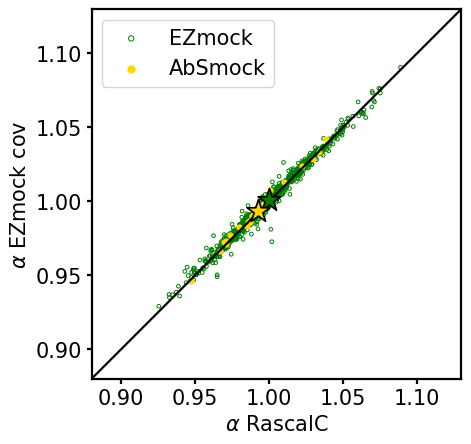
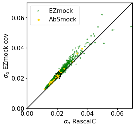
Figure 6: Scatter plots showing the BAO detection significance in units of standard deviations (left panels), the $\alpha$’s (middle panels), and the $\sigma_{\alpha}$ values (right panels) related to the validation procedure of the RascalC-based covariance. BAO best fits are performed on a mock-by-mock basis, using 1000 LRG EZmocks (open green dots) and 25 AbacusSummit LRG realizations (filled yellow points). Stars of the same color are averages over the corresponding entire set of realizations. Top panels refer to pre-reconstruction measurements, while bottom panels display post-reconstruction quantities. Individual BAO fits using the RascalC covariance calibrated on EZmocks (i.e., RascalC-EZ; $x$-axes) are contrasted with those performed adopting the EZmock covariance (i.e., DESI-M2-EZ; $y$-axes). As evident from the figure, the narrow scatter along the diagonal implies that both covariances produce compatible results, validating the usage of RascalC-based covariances for our primary DESI-M2 BAO fits.

The primary BAO fits performed in our main analysis are obtained with semi-analytical semi-empirical covariance matrices, generated by the RascalC code (Philcox et al., 2020). As mentioned in Section 3.3, this choice is mainly driven by the fact that the galaxy mocks available at the time of this study – implementing all of the DESI-M2 survey characteristics – have been calibrated with an earlier version of the DESI LRG clustering (i.e., the One Percent Survey), rather than with the LRG clustering as measured directly from the DESI-M2 dataset considered here. Nevertheless, we also construct a numerical covariance from 1000 LRG EZmocks (termed ‘DESI-M2-EZ’), and use it for validating the LRG RascalC semi-analytical covariance in terms of BAO fitting. In order to calibrate the RascalC covariance matrix for LRGs, besides the previous numerical covariance, we also utilize a covariance directly constructed from the jackknife estimates of the LRG sample under consideration. Once the RascalC semi-analytical covariance is validated (in terms of BAO fits) for the LRG sample, we build a similar semi-empirical covariance for BGS galaxies and calibrate it using jackknife estimates obtained from the corresponding BGS dataset. Table 2 reports all of the covariance matrices utilized in this work. Specifically, in terms of name conventions, we indicate with ‘RascalC-EZ’ the semi-analytical covariance based on the EZmocks LRG clustering, with ‘RascalC-LRG’ the semi-empirical covariance calibrated on the DESI-M2 LRG clustering measurements (including jackknife), and with ‘RascalC-BGS’ the one based on the DESI-M2 BGS clustering.

Next, we provide some additional information on RascalC-based covariances, and then present the BAO fitting validation tests performed on the mock LRG sample.

5.2 RascalC Covariances

The semi-analytical semi-empirical covariance matrices used in our analysis are obtained via the publicly available code RascalC (Philcox et al., 2020; Rashkovetskyi et al., 2023). The procedure to construct such covariances only requires a two-point correlation function as input (along with its optional jackknife estimates), and a random catalog. The RascalC algorithm integrates the Gaussian terms for the covariance matrix using importance sampling from the set of random points. It then progressively changes the amount of shot noise, which has the effect of empirically rescaling those terms. The optimization of the shot noise level is performed on separate jackknife covariance estimates. Once the optimal shot noise level is determined (i.e., its best-fit value), a rescaling based on such best-fit is applied to finally obtain the full covariance matrix terms.

For the construction of the RascalC-LRG and RascalC-BGS covariances (i.e., the covariances calibrated on the DESI-M2 dataset), the input correlation functions are measured directly from the DESI-M2 LRG and BGS samples, respectively. In addition, 60 jackknife regions are assigned based on data points with a K-means subsampler. For the pre-reconstruction case, the RascalC  code is run on 10 random catalogs separately, and the integration results are finally averaged. Building the post-reconstruction covariances calibrated on the DESI-M2 dataset requires some additional steps, described in detail in Rashkovetskyi et al. (2023). In essence, such procedure depends upon the usage of non-shifted random catalogs for normalization, shifted random catalogs for sampling, and a slightly different two-point correlation function than the familiar LS estimator (i.e., Equation 2). In this latter case, the code is run on 20 random catalogs separately, and integration results are eventually averaged.

In order to build the RascalC-EZ covariance, we use instead the averaged pre- and post-reconstructed LRG EZmock correlation functions obtained from 1000 EZmocks, without jackknife estimates, and with no shot-noise rescaling (Gaussian). We run the RascalC code on 10 concatenated random catalogs in pre-reconstrution, and on 20 randoms for the post-reconstruction case.

As concluding remarks for this section, we note that, by construction, the LRG RascalC data covariance (i.e., RascalC-LRG) gives larger error bars than the DESI-M2-EZ sample covariance, while the RascalC covariance based on the EZmock clustering (i.e., RascalC-EZ) is consistent with the DESI-M2-EZ sample covariance. A more detailed assessment on the performance of RascalC-based covariances is presented in Rashkovetskyi et al. (2023).

5.3 Validation of RascalC Covariances for BAO Fitting

Before performing BAO fits on the DESI-M2 dataset, we validate our LRG RascalC covariance against a set of approximate LRG EZmocks and $N$-body based AbacusSummit realizations. While the following tests are performed on LRGs, we note that the validation procedure is general and would apply to any tracers.

Specifically, we first compute the two-point clustering statistics of 1000 LRG EZmocks and 25 AbacusSummit LRG realizations with the estimator presented in Section 4.1, adopting default FKP weights. We then apply the reconstruction algorithm detailed in Section 4.2 to all of the mocks, assuming a smoothing scale of $15h^{-1}{\rm Mpc}$. After, we build the pre- and post-reconstruction EZmock covariance (i.e., DESI-M2-EZ; Table 2), and a RascalC covariance (i.e., RascalC-EZ; Table 2), which is based on the exact average clustering inferred from the entire set of pre- and post-reconstruction LRG EZmocks. Finally, we use both covariances to fit 1000 individual EZmocks as well as 25 individual AbacusSummit realizations with the fitting procedure explained in Section 4.3, within the spatial range $50-150h^{-1}{\rm Mpc}$. In essence, we quantify the BAO best fits and relative errors on a mock-by-mock basis.

Figure 6 shows the results of such a validation test. Top panels refer to pre-reconstruction measurements, while bottom panels display post-reconstruction quantities. From left to right, we report the BAO detection significances in units of standard deviations, and the $\alpha$ and $\sigma_{\alpha}$ values for all of the individual fits performed to the two sets of mocks using the RascalC-EZ covariance ($x$-axes), against the corresponding values obtained with the DESI-M2-EZ covariance ($y$-axes). Open green dots display LRG EZmocks measurements, while filled yellow dots are for AbacusSummit LRG synthetic catalogs. Stars of the same color represent averages over the corresponding entire set of realizations. As evident from the figure, the scatter along the diagonal is quite narrow (both for the pre- and post-reconstruction cases), implying that the two covariances produce compatible results. Moreover, the average values in the various panels are almost overlapping, strongly confirming the consistency between RascalC and mock sample covariances.

A further validation test is reported in Figure 7, where we show the histograms of ($\alpha-\langle\alpha\rangle)/\sigma_{\alpha}$, with $\langle\alpha\rangle$ the mean of the scaling parameter, measured from the $\xi(s)$’s of the pre- (top panel) and post-reconstruction (bottom panel) LRG mocks. This quantity represents an approximation for the signal-to-noise ratio (SNR) of the BAO measurement. Here, we use the $\chi^{2}$ test to assess the validity of the covariances. In essence, we compare the observed scatter in the best-fitting $\alpha$ for the 1000 LRG EZmocks to the $\sigma_{\alpha}$ estimated in each individual fit from the $\Delta\chi^{2}(\alpha)$ curve. Red lines and histograms refer to measurements performed on the EZmock set using the RascalC-EZ covariance, while blue lines and histograms correspond to analogous measurements done assuming the numerically-based DESI-M2-EZ covariance. Results are compared with Gaussian distributions, showing good agreement, as confirmed by near-zero Kolmogorov-Smirnov (K-S) $D_{n}$ tests. Moreover, the corresponding $p$-values imply that our values are drawn from a Gaussian distribution, and that the values of $\sigma_{\alpha}$ we measure from the $\chi^{2}$ distribution are faithful descriptors of the error on $\alpha$ measured by fitting $\xi(s)$. Once again, this test represents another confirmation of the validity of our semi-analytical semi-empirical RascalC-EZ covariance, which produces results compatible with the numerical case.

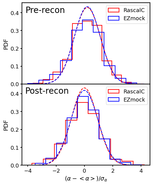
Figure 7: Histograms of ($\alpha-\langle\alpha\rangle)/\sigma_{\alpha}$, with $\langle\alpha\rangle$ the mean of the scaling parameter, measured from the $\xi(s)$’s of the pre- (top panel) and post-reconstruction (bottom panel) LRG mocks. Measurements are performed on 1000 LRG EZmocks, assuming the RascalC-EZ covariance (red lines and histograms), or a numerically-based DESI-M2-EZ covariance (blue lines and histograms). Results are then compared with Gaussian distributions, showing good agreement, and indicating that the values of $\sigma_{\alpha}$ we measure from the $\chi^{2}$ distribution are faithful descriptors of the error on $\alpha$ measured by fitting $\xi(s)$. This test represents a further validation of our semi-analytical RascalC-EZ covariance, which produces results compatible with the numerical one.

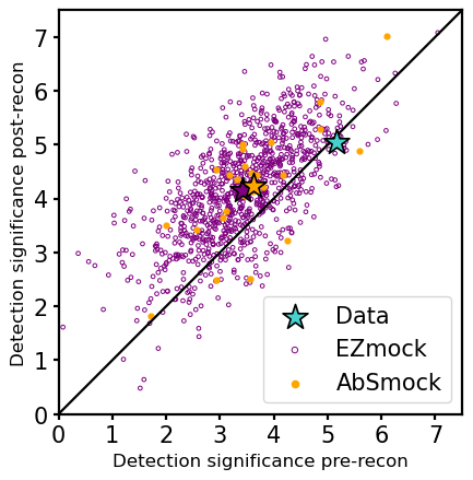
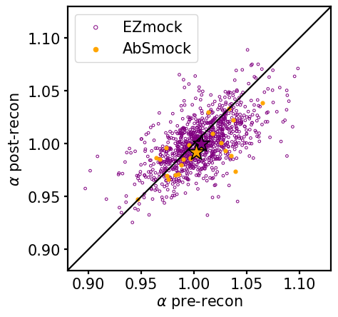
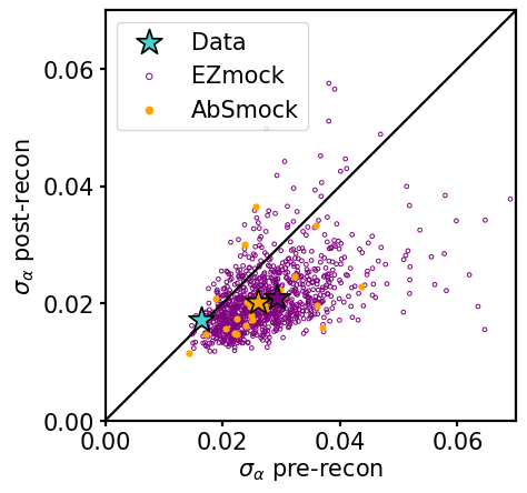
Figure 8: Scatter plots for the BAO detection significance in units of standard deviations (left panel), $\alpha$’s (middle panel), and $\sigma_{\alpha}$’s (right panel), addressing the effect of reconstruction on the BAO fitting procedure for the LRG sample. Results are obtained from individual correlation function fits performed to 1000 LRG EZmocks (open purple dots) and 25 AbacusSummit LRG synthetic catalogs (filled orange dots). Stars of identical color represent averages over the corresponding entire set of realizations. Pre- ($x$-axes) and post-reconstruction ($y$-axes) measurements are compared, adopting the RascalC-EZ covariance. While reconstruction increases considerably the BAO detection significance for the mocks, the same procedure applied to the DESI-M2 LRG sample produces only marginal effects: the cyan stars in the left and right panels are DESI-M2 LRG measurements obtained via a RascalC covariance calibrated directly on LRGs, pointing to a ‘lucky’ realization in the upper right corner of the significance scatter plot (left panel), and in the lower left corner of the $\sigma_{\alpha}$ plot (right panel), respectively. This situation is similar to those reported for BOSS CMASS LRGs (Anderson et al., 2012), and for the eBOSS LRG sample (Bautista et al., 2021).

In summary, the tests performed in this section clearly prove that using a RascalC-based covariance returns unbiased and consistent estimates when compared to results obtained with the numerical EZmock covariance. We can then safely proceed to tune our RascalC covariance to match the clustering inferred from the DESI-M2  datasets, and perform the key BAO fits on the LRG and BGS samples – as we describe in the next section.

6 Key Results: BAO Signal Detection

In this section, we present the main results of our DESI-M2 analysis, and assess the precision and detection statistics of the BAO feature both in the LRG and BGS samples. We do not report here the best fit BAO scales as inferred from actual data, since the cosmology is intentionally kept blinded. Our focus is primarily on LRGs, as they are characterized by the highest SNR among the four DESI-M2 tracers.

6.1 BAO Reconstruction Efficiency

Before performing BAO fits to the DESI-M2 dataset, we first address the effect of BAO reconstruction on the BAO fitting procedure – focusing on the LRG sample. In Figure 8, we report the BAO detection significances expressed in units of standard deviations, as well as the $\alpha$ and $\sigma_{\alpha}$ values from all of the individual correlation function fits performed to the two sets of LRG mocks previously considered. Specifically, we compare pre- ($x$-axes) and post-reconstruction ($y$-axes) measurements, obtained by adopting the RascalC-EZ covariance. Open purple dots display EZmocks LRG results, while filled orange dots are for the AbacusSummit LRG synthetic catalogs. Similarly to Figure 6, stars of identical color represent averages over the corresponding entire set of realizations. As evident from the scatter plot, the BAO detection significance (reported in the left panel) increases considerably after reconstruction, and the $\alpha$’s of the mocks are closer to unity after reconstruction (central panel), as expected. Moreover, the errors tend to improve significantly after reconstruction for about 90% of the cases (i.e., right panel). Hence, the reconstruction procedure appears to be efficient on the mocks.

Reconstruction applied to LRG data appears instead to produce only marginal effects. To this end, in Figure 8 we overplot the DESI-M2 LRG measurements (cyan stars in the left and right panels), obtained by using the RascalC-LRG covariance calibrated directly on LRGs. As evident from the figure, the DESI-M2 LRG measurements are located in the upper right corner of the significance scatter plot (left panel), and in the lower left corner of the $\sigma_{\alpha}$ plot (right panel), respectively: hence, we are in a similarly ‘lucky’ situation as those reported for the BOSS CMASS LRG sample by Anderson et al. (2012), and also for eBOSS LRGs (Bautista et al., 2021). Table 4 provides a quantification of the ‘lucky’ realization of the observational data point, showing that both its detection significance and precision are consistent with those obtained via mock averages. In particular, focusing on post-reconstruction results, the detection significance of the data point is 5.050 (in units of standard deviations) with a precision of 1.7%, while the average EZmocks results yield a detection significance of 4.138 with a precision of 2.1%, and from the average of the AbacusSummit mocks we obtain 4.242 with a 2.0% precision. Note that a small $\sigma_{\alpha}$ implies a better BAO detection, thus a higher significance. In essence, while generally reconstruction improves errors on $\alpha$, this may not happen if the starting (pre-reconstruction) point already has a low error to begin with (i.e., a ‘lucky’ realization). In such a situation, reconstruction does not tend to produce much improvement, as shown in the $\sim 10\%$ of the mocks in our analysis. This seems to be the case for the DESI-M2 LRG sample data volume: our recovered $\sigma_{\alpha}$ for data is much smaller than the mean expected from the mocks (right panel), and our BAO detection significance is high (left panel), showing a strong and well-defined acoustic peak.

6.2 BAO Detection from the LRG Sample

Table 3: BAO key fitting results for DESI-M2 LRGs and BGS.

Sample	Reconstruction	BAO Detection Significance	$\alpha+\Delta\alpha$	min$(\chi^{2})$/dof
DESI-M2 LRG	Pre-recon	5.170	0.987 $\pm$ 0.016	15.619 / 20
	Post-recon	5.050	1.000 $\pm$ 0.017	13.463 / 20
DESI-M2 BGS	Pre-recon	2.337	0.980 $\pm$ 0.040	13.172 / 20
	Post-recon	2.963	1.001 $\pm$ 0.026	16.724 / 20

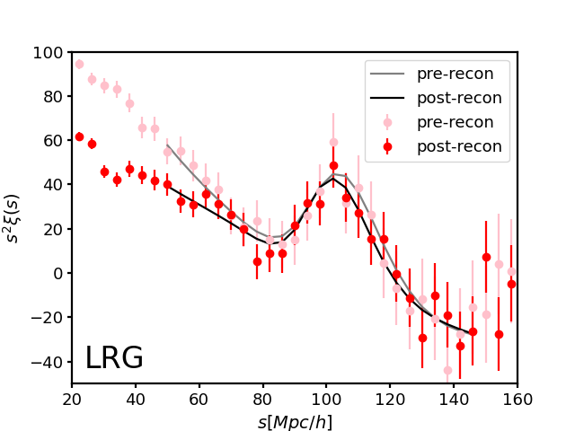
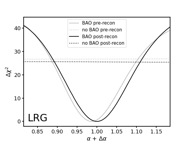
Figure 9: BAO feature and its significance, as detected in the large-scale correlation function of DESI-M2 LRGs. [Left] Pre- (lighter pink dots with errorbars) and post- (red dots with errorbars) reconstruction two-point clustering statistics inferred from the LRG sample, clearly displaying the BAO peak. The gray and black lines are respectively pre- and post-reconstruction fits to $\xi(s)$ in the spatial range $50-150h^{-1}{\rm Mpc}$ over 25 points with 20 dof, obtained using the RascalC-LRG covariance. Errorbars are the square root of its diagonal elements. [Right] Detection significance of the DESI-M2 LRG BAO feature before (lighter gray lines) and after (black lines) reconstruction. Dotted lines with similar colors are corresponding fits to the data using a model without BAO. We have shifted each value of $\alpha$ by $\Delta\alpha$ both in pre- and post-reconstruction, such that the minimum $\chi^{2}$ of the post-reconstruction result is at 1. We note that an identical $\Delta\alpha$ was introduced for post-reconstruction LRGs and BGS (Figure 10), to demonstrate the coherence in terms of cosmological implications from the two tracers at the two different redshifts, while being blinded. The BAO peak is detected at $\sim 5\sigma$ confidence with a $1.6\%$ and $1.7\%$ precision in the pre- and post-reconstruction DESI-M2 LRG sample, respectively, with the reconstruction procedure playing only a marginal role. Such a remarkable detection level, obtained with just two months of DESI operations, is comparable to the one reported for the BOSS CMASS sample (Anderson et al., 2012), and it is quite reassuring – given the high complexity of the DESI instrument and of the DESI spectroscopic reduction pipeline.

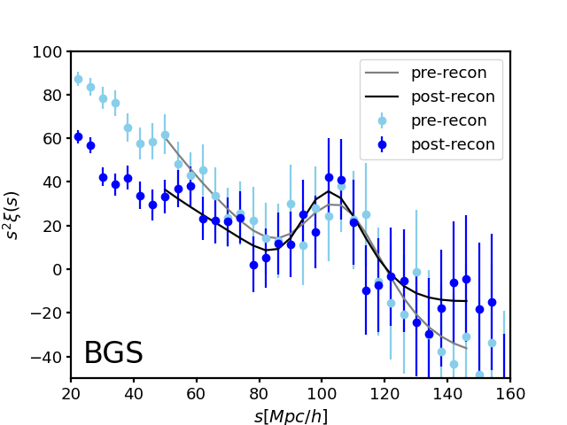
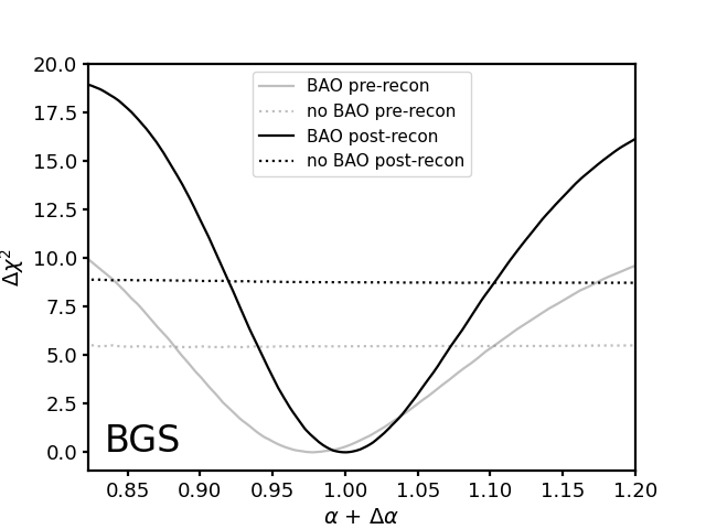
Figure 10: BAO feature and its significance, as detected in the large-scale correlation function of DESI-M2 BGS. Line styles and conventions same as in Figure 9. [Left] Pre- and post-reconstruction two-point clustering statistics inferred from the BGS sample. BAO fits to $\xi(s)$ are performed in the spatial range $50-150h^{-1}{\rm Mpc}$, adopting the RascalC-BGS covariance. Errorbars are the square root of its diagonal elements. [Right] Detection significance of the DESI-M2 BGS BAO feature before (lighter gray lines) and after (black lines) reconstruction. Dotted lines with indentical colors are corresponding fits to the data using a model without BAO. We have shifted each value of $\alpha$ by the same $\Delta\alpha$ both in pre- and post-reconstruction, as done for the LRG analysis. The acoustic feature is detected at $\sim 2.5\sigma$ significance with a $4.0\%$ precision in pre-reconstruction, and at $\sim 3.0\sigma$ with a $2.6\%$ precision in post-reconstruction. Clearly, for this galaxy sample, reconstruction plays a more substantial effect in sharpening the acoustic peak. This BAO detection represents another relevant milestone of our DESI-M2 analysis.

Figure 9 displays the BAO fit to the DESI-M2 LRG two-point correlation function, along with its significance: this measurement represents one of the key results of our analysis. The left panel shows the pre- and post-reconstruction clustering statistics computed with the LS estimator (points with errorbars), and the best-fit model (curves). The gray and black curves are respectively pre- and post-reconstruction fits to $\xi(s)$ in the spatial range $50-150h^{-1}{\rm Mpc}$, obtained with the procedure detailed in Section 4.3 and using the RascalC-LRG covariance matrix: errorbars in the plot show the square root of its diagonal elements. The BAO peak is clearly detected, and well matched to the best-fitting model. This is confirmed quantitatively: we find $\chi^{2}_{\rm min}=15.6$ and $\chi^{2}_{\rm min}=13.5$ for the pre- and post-reconstruction cases assuming 20 dof, respectively. Table 3 reports the specifics of these BAO fits.

The right panel of Figure 9 displays the likelihood for the DESI-M2 LRG BAO scale, as represented by $\Delta\chi^{2}=\chi^{2}-\chi^{2}_{\rm min}$, before and after reconstruction (solid curves). Dotted lines having identical colors represent corresponding fits to the data using a model without BAO. This provides two crucial results: the uncertainty on the measurement, and the significance of the BAO feature. Assuming a Gaussian likelihood, the 1$\sigma$ confidence region is represented by the width of the curve with $\Delta\chi^{2}<1$. We estimate the 1$\sigma$ uncertainty to be 0.016 in pre-reconstruction and 0.017 in post-reconstruction, respectively. The BAO detection significance can be simply determined by comparing results obtained from a fit to the data using a model without BAO (displayed via dotted lines in the figure), and once again subtracting the $\chi^{2}_{\rm min}$ from the BAO fit. This indicates how much better a model containing BAO fits the LRG data (i.e., actual existence of the BAO peak in the galaxy sample). The $\Delta\chi^{2}_{\rm min,noBAO}$ is greater than 25 both in pre- and post-reconstruction. Hence, we report a detection of the BAO feature in the DESI-M2 LRG sample at a significance greater than 5$\sigma$.

We note that we have shifted each $\alpha$ by the corresponding value of $\Delta\alpha$ in the right panel of Figure 9, such that the minimum $\chi^{2}$ is at 1 for the post-reconstruction case. The magnitude of the required shift for the post-reconstruction result was less than 1$\sigma$. Thus, while we do not reveal the precise value of the BAO scale in this analysis, we are consistent with the fiducial cosmology.

As illustrated in Figure 9, the BAO detection in the DESI-M2 LRG sample is highly significant. Such a remarkable detection level, obtained with only two months of DESI operations, is comparable to the one reported for the BOSS high-$z$ LRG sample (i.e., CMASS; Anderson et al., 2012), comprised of 264 283 galaxies in the redshift interval $0.43<z<0.7$. Notice also that the reconstruction procedure has practically no impact on the BAO peak inferred from the DESI-M2 LRG clustering, as evident from the right panel of Figure 9 (compare the gray and black curves). As pointed out in the previous section, this is due to the ‘lucky’ starting point of the pre-reconstruction LRG measurement, which happens to be located in the lower left corner of the $\sigma_{\alpha}$ plot in Figure 8, yielding already a very low error to begin with, and hence carrying a high BAO detection significance (i.e., left panel of the same figure, see the cyan star in the upper right corner of the significance scatter plot).

In closing this section, we emphasize that the first BAO measurement obtained with DESI-M2 LRGs represents an important milestone, and its high detection level is quite reassuring – considering the complexity of the DESI instrument and of the spectroscopic reduction pipeline. It also constitutes an important early validation and quality-control of the data management system, as well as a confirmation of the successful survey design strategy adopted for DESI targets. Next, we move to the BGS sample and carry out a similar BAO analysis.

6.3 BAO Detection from the BGS

Figure 10 contains another central result of our analysis. Here, we report the BAO feature as detected in the large-scale clustering of the DESI-M2 BGS BRIGHT sample characterized by a magnitude cut of $-21.5$ (see Section 2), together with its significance. In detail, the left panel displays two-point correlation function measurements from those galaxies. Following similar conventions as in Figure 9, the gray and black curves are respectively the pre- and post-reconstruction best-fit models to $\xi(s)$ in the spatial range $50-150h^{-1}{\rm Mpc}$, obtained using the RascalC-BGS covariance matrix. Errorbars in the plot show the square root of its diagonal elements. Also in this case, the BAO peak is clearly detected and well matched to the best-fitting model. Specifically, $\chi^{2}_{\rm min}=13.2/20~{}{\rm dof}$ in pre-reconstruction, and $\chi^{2}_{\rm min}=16.7/20~{}{\rm dof}$ in post-reconstruction. See again Table 3 for details on these BAO fits.

The right panel of Figure 10 shows the likelihood for the DESI-M2 BGS BRIGHT BAO scale before and after reconstruction (solid lines). Dotted lines with identical colors represent the corresponding fits to the data using a model without BAO. Similarly to the LRG analysis, we determine the 1$\sigma$ confidence region of the measurements based on the width of the curve with $\Delta\chi^{2}<1$. This yields an uncertainty of $0.040$ in pre-reconstruction, and of $0.026$ in post-reconstruction. As evident by comparing the gray and black curves from both panels of Figure 10, here reconstruction plays a more substantial effect in sharpening the acoustic peak and in partially removing the BAO smearing caused by non-linear structure growth. By comparing the $\chi^{2}$ of the data fits against a model without BAO, we determine the significance of the BAO feature. We find $\Delta\chi^{2}$ to be 5.5 in pre-reconstruction and 8.8 in post-reconstruction, corresponding to a BAO detection significance of $\sim 2.3\sigma$ and $\sim 3.0\sigma$, respectively.

Even for the DESI-M2 BGS sample, we have shifted the individual $\alpha$’s by the same $\Delta\alpha$ factor applied to the LRG sample, both in pre- and post-reconstruction. Since the BGS minimum $\chi^{2}$ values are within $1\sigma$ of $\alpha+\Delta\alpha=1$, we can conclude that the BGS BAO results are fully consistent with the LRG ones.

Along with the first BAO measurement from the DESI-M2 LRG sample, this first BAO detection obtained using the DESI-M2 BGS represents another relevant milestone, as well as an additional early validation of the DESI pipeline and data management system for the bright time survey.

7 Outlook for Future Data Releases

Based on the promising BAO results presented in Section 6, obtained with the DESI-M2 dataset collected over just two months of operations, we now proceed to forecast the expected BAO detection significance and accuracy with the completed survey data, focusing on the final Y5 DESI LRG sample.

To this end, we compute Fisher matrix forecasts of the LRG isotropic BAO scale. We perform such calculations by adopting covariance matrices constructed using post-reconstruction EZmocks for the two survey configurations (i.e., DESI-M2 LRGs and DESI Y5 LRGs, respectively) and the best-fit monopole model for DESI-M2 – while marginalizing over the same free parameters as in the actual data fit. We then take the ratio of the two Fisher estimates to rescale the DESI-M2 constraint, in order to account for the specific calibration of the LRG EZmocks, tuned on the One Percent Survey clustering rather than on DESI-M2  (see again Section 3.3 for details). These Fisher estimates return a factor of $\sim 5.8$ between the BAO SN inferred from Y5 LRGs and that of DESI-M2 LRGs. When we rescale our data best-fit LRG estimate of $1.7\%$ accounting for this factor, we then predict a $\sim 0.29\%$ precision on the BAO scale from the final Y5 LRG sample over $0.4<z<1.1$.

We note that such estimate should be taken as an approximate projection for DESI Y5, since we have simply assumed the same BAO signal from DESI-M2 while only changing the covariance. Nevertheless, the projected BAO precision for DESI Y5 LRGs agrees well with the more accurate DESI LRG Y5 forecasts based on GoFish – i.e., 0.25% precision for the DESI Y5 LRG sample, presented in DESI Collaboration et al. (2023a). This exquisite level of sub-percent precision on the BAO scale (even from a single tracer) will confirm DESI as the most competitive BAO experiment for the remainder of this decade.

8 Conclusions

The BAO scale represents a key standard ruler that provides a direct way to measure the expansion history of the Universe and infer robust cosmological constraints. Hence, BAO measurements are considered primary DESI science targets, and a major deliverable at any stage of the survey. Precision on the expansion history of the Universe constitutes a compelling probe of the nature of DE. DESI is expected to deeply impact the current understanding of DE, along with providing unprecedented constrain on theories of modified gravity and inflation, and on neutrino masses (DESI Collaboration et al., 2016). In this respect, DESI plans to conduct a series of BAO analyses throughout its five-year survey time with blinded catalogs: the Y1 sample would be the first of such rigorously blinded BAO analyses.

The remarkable complexity of the DESI instrument, along with the adopted survey design and the elaborated DESI spectroscopic pipeline and data management system, pose a potential challenge to all BAO analyses. It is then of utmost importance to test such pipelines well in advance, and it has been the main goal of the current study: this is a crucial aspect in order to guarantee the success of future BAO investigations, and for confirming the optimal performance of the DESI spectrograph and the quality level of the data reduction pipeline. Precisely for this reason, the first two months of DESI operations were intentionally kept unblinded (i.e., DESI-M2 sample).

To this end, we have used the DESI-M2 dataset and reported the first high-significance detection of the BAO signal from the LRG and BGS samples. Specifically, our primary results are:

• $\sim 5\sigma$ level BAO detection in the DESI-M2 LRG sample at a precision of $1.7\%$.

• $\sim 3\sigma$ level BAO detection in the DESI-M2  BGS sample at a precision of $2.6\%$.

In particular, our LRG BAO measurement is comparable to the $5-6\sigma$ BAO detection obtained with the BOSS high-$z$ LRG sample (i.e., CMASS; Anderson et al., 2012), comprised of 264,283 galaxies in the redshift interval $0.43<z<0.7$. Moreover, the BOSS and eBOSS BAO measurements made with LRGs between $0.4<z<1.0$ (with $N_{\rm gal}=1{,}063{,}828$) returned an aggregate precision of 0.77% on $D_{\rm V}$ (Bautista et al., 2021), which is only a factor of $2.2$ times better (in terms of precision) than our quoted result with DESI-M2 LRGs (having just $N_{\rm gal}=266,269$). This latter aspect is rather remarkable, considering that the DESI-M2 dataset has been collected simply during the initial two months of DESI operations.

Based on these results, we forecasted that DESI is on target to achieve a high-significance BAO detection at a $\sim 0.29\%$ precision with the completed Y5 LRG sample over $0.4<z<1.1$, meeting the DESI top-level science requirements on BAO measurements. This exquisite level of precision will set novel standards in cosmology and confirm DESI as a highly accurate and precise Stage-IV BAO experiment.

Additional relevant aspects of our investigation on these preliminary DESI-M2 data that are worth highlighting are summarized as follows:

• Although the catalogs we used are unblinded, we presented a blinded cosmology analysis – in that we do not report here the best fit BAO scale. In fact, we only presented the precision and detection level of the BAO measurements. We plan to provide a full cosmological interpretation with the Y1 data release in the near future, after additional rigorous systematic tests.

• We focused on the isotropic BAO scale exploiting only the monopole of the LRG and BGS samples.

• We applied the nominal BAO pipeline that has been previously well-tested with BOSS and eBOSS data. In particular, we utilized the early version of the pipeline package cosmodesi that the DESI collaboration team has been developing, which wraps both existing and new cosmological galaxy survey analysis pipelines from the literature.

• We constructed, calibrated, and used semi-analytical semi-empirical covariance matrices based on the RascalC code, and validated those covariances in terms of BAO fitting procedures (in pre- and post-reconstruction) using a set of mocks – as detailed in Section 5 and in Rashkovetskyi et al. (2023).

• We also found that the LRG BAO signal from the DESI-M2 data is stronger than the typical BAO signal present in the LRG mocks. Partly for this reason, the reconstruction procedure performed on actual LRG data is less effective than the one performed on LRG mocks. On the other hand, we found that the BGS sample shows a factor of $\sim 1.5$ precision improvement after reconstruction. These results are consistent with the typical behavior we find on DESI-M2 mocks; less scatter is expected for the more complete DESI Y1 and Y5 samples.

This work represents the first step towards the analysis techniques that will lead to the key cosmological results from DESI Y1 data. While the BAO results presented here constitute an important milestone and are quite reassuring in terms of consistency in the clustering amplitude (considering the complexity of the DESI instrument and of the spectroscopic reduction pipeline), we anticipate that the DESI Y1 analysis alone will surpass the cosmological information from all of the BAO analyses performed to date. This will require going beyond the legacy BAO analysis setting that has been well-tested using BOSS and eBOSS data (and also mainly adopted here), with an unprecedented level of BAO systematic tests and by developing an optimal BAO pipeline – given the stringent requirements on theoretical and observational systematics that are imposed by a dataset as powerful as we expect by the end of the survey. The DESI team is currently working in this direction, and presenting all these novel technical aspects will be the subject of many forthcoming DESI Y1 cosmology papers.

Data Availability

The redshift measurements used in this paper – derived from the DESI Guadalupe dataset – will be made public with the DESI Y1 data release (DR1). The analogous spectroscopic data reductions and redshift fits for the DESI EDR (i.e., Fuji) will be publicly available on NERSC at this url: https://data.desi.lbl.gov/public/edr/spectro/redux/fuji. All data points shown in the published graphs are available in machine-readable form in Zenodo at https://doi.org/10.5281/zenodo.7835433.

Appendix A Supporting Material

Table 4: BAO key fitting results for LRGs. For DESI-M2 LRGs, we use the RascalC-LRG covariance, while for the two sets of mocks we applied instead the RascalC-EZ covariance – see Section 5 and Table 2 for details. We do not show here the $\alpha$ values for the LRG data fits, as the cosmology is kept blinded. Moreover, we do not report DESI-M2 fits with the EZmock numerical covariance, since EZmocks are calibrated with the One Percent Survey data (as explained in Section 3.3).

	Reconstruction	BAO results	RascalC cov	EZmock cov
	Pre-recon	Detection significance	5.170	–
DESI-M2 LRG		Precision	1.6%	–
	Post-recon	Detection significance	5.050	–
		Precision	1.7%	–
		Detection significance	3.423	3.597
	Pre-recon	$\alpha$	1.006	1.006
EZmock LRG		Precision	2.8%	2.7%
		Detection significance	4.138	4.091
	Post-recon	$\alpha$	1.000	1.001
		Precision	2.1%	2.3%
		Detection significance	3.623	3.801
	Pre-recon	$\alpha$	1.001	0.997
AbSmock LRG		Precision	2.8%	2.5%
		Detection significance	4.242	4.209
	Post-recon	$\alpha$	0.992	0.994
		Precision	2.0%	2.1%

In support of the primary BAO analysis carried out in the main text, in Table 4 we provide some further technical details related to the various BAO fits performed to the DESI-M2 LRG sample, as well as to the corresponding LRG mocks adopted in this work – namely, pre- an post-reconstruction results of the BAO detection significance and precision, along with the $\alpha$ values for the mock fits. Specifically, as reported in the main text, the DESI-M2 LRG sample provides a $\sim 5\sigma$ BAO detection significance at a 1.6% and 1.7% precision in pre- and post-reconstruction, respectively. From the two sets of mocks considered (AbacusSummit and EZmocks), we also find a significant BAO detection at more than 3.4 $\sigma$ in pre-reconstruction, and exceeding a 4.0 $\sigma$ detection in post-reconstruction, with a corresponding precision better than 2.8% (pre-reconstruction) or 2.3% (post-reconstruction). Remarkably, the $\alpha$-values inferred from the mocks are close to unity, indicating that the fiducial cosmology is very-well recovered. This also implies that the mock production pipeline is working properly. Additionally, from Table 4 one can readily infer that the RascalC-based LRG covariance is compatible with the EZmock LRG covariance (as we also reported in Section 5), simply by comparing all the corresponding fitting results obtained with the two sets of covariances (i.e., last two columns).

¹Department of Physics and Astronomy, Sejong University, Seoul, 143-747, Korea
²Department of Physics & Astronomy, Ohio University, Athens, OH 45701, USA
³Center for Astrophysics $|$ Harvard & Smithsonian, 60 Garden Street, Cambridge, MA 02138, USA
⁴Korea Astronomy and Space Science Institute, 776 Daedeok-daero, Yuseong-gu, Daejeon 34055, Republic of Korea
⁵Lawrence Berkeley National Laboratory, 1 Cyclotron Road, Berkeley, CA 94720, USA
⁶Physics Dept., Boston University, 590 Commonwealth Avenue, Boston, MA 02215, USA
⁷Tata Institute of Fundamental Research, Homi Bhabha Road, Mumbai 400005, India
⁸Physics Department, Yale University, P.O. Box 208120, New Haven, CT 06511, USA
⁹NSF’s NOIRLab, 950 N. Cherry Ave., Tucson, AZ 85719, USA
¹⁰Department of Physics & Astronomy, University College London, Gower Street, London, WC1E 6BT, UK
¹¹IRFU, CEA, Université Paris-Saclay, F-91191 Gif-sur-Yvette, France
¹²Department of Physics and Astronomy, The University of Utah, 115 South 1400 East, Salt Lake City, UT 84112, USA
¹³Instituto de Física, Universidad Nacional Autónoma de México, Cd. de México C.P. 04510, México
¹⁴Department of Physics, Southern Methodist University, 3215 Daniel Avenue, Dallas, TX 75275, USA
¹⁵Fermi National Accelerator Laboratory, PO Box 500, Batavia, IL 60510, USA
¹⁶Institut de Física dAltes Energies (IFAE), The Barcelona Institute of Science and Technology, Campus UAB, 08193 Bellaterra Barcelona, Spain
¹⁷Departamento de Física, Universidad de los Andes, Cra. 1 No. 18A-10, Edificio Ip, CP 111711, Bogotá, Colombia
¹⁸Department of Physics, The University of Texas at Dallas, Richardson, TX 75080, USA
¹⁹University of Michigan, Ann Arbor, MI 48109, USA
²⁰Department of Physics, The Ohio State University, 191 West Woodruff Avenue, Columbus, OH 43210, USA
²¹Center for Cosmology and AstroParticle Physics, The Ohio State University, 191 West Woodruff Avenue, Columbus, OH 43210, USA
²²Department of Physics, Southern Methodist University, 3215 Daniel Avenue, Dallas, TX 75275, USA
²³Natural Science Research Institute, University of Seoul, 163 Seoulsiripdae-ro, Dongdaemun-gu, Seoul, South Korea
²⁴Sorbonne Université, CNRS/IN2P3, Laboratoire de Physique Nucléaire et de Hautes Energies (LPNHE), FR-75005 Paris, France
²⁵Departament de Física, Serra Húnter, Universitat Autònoma de Barcelona, 08193 Bellaterra (Barcelona), Spain
²⁶Department of Astronomy, The Ohio State University, 4055 McPherson Laboratory, 140 W 18th Avenue, Columbus, OH 43210, USA
²⁷Institució Catalana de Recerca i Estudis Avançats, Passeig de Lluís Companys, 23, 08010 Barcelona, Spain
²⁸Department of Physics and Astronomy, Siena College, 515 Loudon Road, Loudonville, NY 12211, USA
²⁹Department of Physics & Astronomy, University of Wyoming, 1000 E. University, Dept. 3905, Laramie, WY 82071, USA
³⁰Institute of Cosmology & Gravitation, University of Portsmouth, Dennis Sciama Building, Portsmouth, PO1 3FX, UK
³¹Institute for Astronomy, University of Edinburgh, Royal Observatory, Blackford Hill, Edinburgh EH9 3HJ, UK
³²Department of Physics & Astronomy and Pittsburgh Particle Physics, Astrophysics, and Cosmology Center (PITT PACC), University of Pittsburgh, 3941 O’Hara Street, Pittsburgh, PA 15260, USA
³³National Astronomical Observatories, Chinese Academy of Sciences, A20 Datun Rd., Chaoyang District, Beijing, 100012, P.R. China
³⁴Waterloo Centre for Astrophysics, University of Waterloo, 200 University Ave W, Waterloo, ON N2L 3G1, Canada
³⁵Perimeter Institute for Theoretical Physics, 31 Caroline St. North, Waterloo, ON N2L 2Y5, Canada
³⁶Space Sciences Laboratory, University of California, Berkeley, 7 Gauss Way, Berkeley, CA 94720, USA
³⁷GMT RPG - Campus de Excelencia Internacional CIE/UAM + CSIC, Universidad Autónoma de Madrid
³⁸Department of Physics, Kansas State University, 116 Cardwell Hall, Manhattan, KS 66506, USA
³⁹Ecole Polytechnique Fédérale de Lausanne, CH-1015 Lausanne, Switzerland
⁴⁰Department of Physics, University of California, Berkeley, 366 LeConte Hall MC 7300, Berkeley, CA 94720-7300, USA
⁴¹SLAC National Accelerator Laboratory, Menlo Park, CA 94305, USA

References

- Abareshi et al. (2022) Abareshi B., et al., 2022, AJ, 164, 207
- Alcock & Paczynski (1979) Alcock C., Paczynski B., 1979, Nature, 281, 358
- Anderson et al. (2012) Anderson L., et al., 2012, MNRAS, 427, 3435
- Ata et al. (2018) Ata M., et al., 2018, MNRAS, 473, 4773
- Bautista et al. (2021) Bautista J. E., et al., 2021, MNRAS, 500, 736
- Blake et al. (2012) Blake C., et al., 2012, MNRAS, 425, 405
- Blanton et al. (2017) Blanton M. R., et al., 2017, AJ, 154, 28
- Brieden et al. (2020) Brieden S., Gil-Marín H., Verde L., Bernal J. L., 2020, J. Cosmology Astropart. Phys., 2020, 052
- Burden et al. (2015) Burden A., Percival W. J., Howlett C., 2015, MNRAS, 453, 456
- Carter et al. (2020) Carter P., Beutler F., Percival W. J., DeRose J., Wechsler R. H., Zhao C., 2020, MNRAS,
- Chaussidon et al. (2021) Chaussidon E., et al., 2021, Mon. Not. Roy. Astron. Soc., 509, 3904
- Chaussidon et al. (2023) Chaussidon E., et al., 2023, ApJ, 944, 107
- Chuang et al. (2015) Chuang C.-H., Kitaura F.-S., Prada F., Zhao C., Yepes G., 2015, MNRAS, 446, 2621
- Cole et al. (2005) Cole S., et al., 2005, MNRAS, 362, 505
- Cooper et al. (2022) Cooper A. P., et al., 2022, arXiv e-prints, p. arXiv:2208.08514
- DESI Collaboration et al. (2016) DESI Collaboration et al., 2016, arXiv e-prints, p. arXiv:1611.00036
- DESI Collaboration et al. (2023a) DESI Collaboration et al., 2023a, arXiv e-prints, p. arXiv:2306.06307
- DESI Collaboration et al. (2023b) DESI Collaboration et al., 2023b, arXiv e-prints, p. arXiv:2306.06308
- Dark Energy Survey Collaboration et al. (2022) Dark Energy Survey Collaboration et al., 2022, Phys. Rev. D, 105, 023520
- Dawson et al. (2016) Dawson K. S., et al., 2016, AJ, 151, 44
- Eisenstein et al. (2005) Eisenstein D. J., et al., 2005, ApJ, 633, 560
- Eisenstein et al. (2007) Eisenstein D. J., Seo H.-J., Sirko E., Spergel D. N., 2007, ApJ, 664, 675
- Feldman et al. (1994) Feldman H. A., Kaiser N., Peacock J. A., 1994, Astrophys. J., 426, 23
- Gaia Collaboration et al. (2018) Gaia Collaboration et al., 2018, A&A, 616, A1
- Górski et al. (2005) Górski K. M., Hivon E., Banday A. J., Wandelt B. D., Hansen F. K., Reinecke M., Bartelmann M., 2005, ApJ, 622, 759
- Guy et al. (2023) Guy J., et al., 2023, Astron. J., 165, 144
- Hahn et al. (2023) Hahn C., et al., 2023, AJ, 165, 253
- Hou et al. (2020) Hou J., et al., 2020, Mon. Not. Roy. Astron. Soc., 500, 1201
- Kaiser (1987) Kaiser N., 1987, Mon. Not. Roy. Astron. Soc., 227, 1
- Landy & Szalay (1993) Landy S. D., Szalay A. S., 1993, ApJ, 412, 64
- Maksimova et al. (2021) Maksimova N. A., Garrison L. H., Eisenstein D. J., Hadzhiyska B., Bose S., Satterthwaite T. P., 2021, MNRAS, 508, 4017
- Myers et al. (2023) Myers A. D., et al., 2023, AJ, 165, 50
- Padmanabhan et al. (2012) Padmanabhan N., Xu X., Eisenstein D. J., Scalzo R., Cuesta A. J., Mehta K. T., Kazin E., 2012, MNRAS, 427, 2132
- Percival et al. (2014) Percival W. J., et al., 2014, MNRAS, 439, 2531
- Philcox et al. (2020) Philcox O. H. E., Eisenstein D. J., O’Connell R., Wiegand A., 2020, MNRAS, 491, 3290
- Planck Collaboration et al. (2020) Planck Collaboration et al., 2020, A&A, 641, A6
- Raichoor et al. (2020) Raichoor A., et al., 2020, Mon. Not. Roy. Astron. Soc., 500, 3254
- Raichoor et al. (2023) Raichoor A., et al., 2023, AJ, 165, 126
- Rashkovetskyi et al. (2023) Rashkovetskyi M., et al., 2023, MNRAS, 524, 3894
- Ross et al. (2017) Ross A. J., et al., 2017, Mon. Not. Roy. Astron. Soc., 464, 1168
- Ross et al. (2020) Ross A. J., et al., 2020, Mon. Not. Roy. Astron. Soc., 498, 2354
- Schlafly et al. (2023) Schlafly E. F., et al., 2023, arXiv e-prints, p. arXiv:2306.06309
- Schlegel et al. (1998) Schlegel D. J., Finkbeiner D. P., Davis M., 1998, ApJ, 500, 525
- Seo et al. (2016) Seo H.-J., Beutler F., Ross A. J., Saito S., 2016, MNRAS, 460, 2453
- Silber et al. (2022) Silber J. H., et al., 2022, The Astronomical Journal, 165, 9
- Sinha & Garrison (2019) Sinha M., Garrison L., 2019, in Majumdar A., Arora R., eds, Software Challenges to Exascale Computing. Springer Singapore, Singapore, pp 3–20, https://doi.org/10.1007/978-981-13-7729-7_1
- Sinha & Garrison (2020) Sinha M., Garrison L. H., 2020, MNRAS, 491, 3022
- Vargas-Magaña et al. (2018) Vargas-Magaña M., et al., 2018, MNRAS, 477, 1153
- Wallisch (2018) Wallisch B., 2018, PhD thesis, Cambridge U. (arXiv:1810.02800), doi:10.17863/CAM.30368
- Weinberg et al. (2013) Weinberg D. H., Mortonson M. J., Eisenstein D. J., Hirata C., Riess A. G., Rozo E., 2013, Phys. Rep., 530, 87
- Xu et al. (2012) Xu X., Padmanabhan N., Eisenstein D. J., Mehta K. T., Cuesta A. J., 2012, Mon. Not. Roy. Astron. Soc., 427, 2146
- York et al. (2000) York D. G., et al., 2000, AJ, 120, 1579
- Zel’dovich (1970) Zel’dovich Y. B., 1970, Astrofizika, 6, 319
- Zhao et al. (2021) Zhao C., et al., 2021, MNRAS, 503, 1149
- Zhou et al. (2023) Zhou R., et al., 2023, AJ, 165, 58
- du Mas des Bourboux et al. (2020) du Mas des Bourboux H., et al., 2020, ApJ, 901, 153
- eBOSS Collaboration et al. (2021) eBOSS Collaboration et al., 2021, Phys. Rev. D, 103, 083533