ATHEENA: A Toolflow for Hardware Early-Exit Network Automation

Abstract

The continued need for improvements in accuracy, throughput, and efficiency of Deep Neural Networks has resulted in a multitude of methods that make the most of custom architectures on FPGAs. These include the creation of hand-crafted networks and the use of quantization and pruning to reduce extraneous network parameters. However, with the potential of static solutions already well exploited, we propose to shift the focus to using the varying difficulty of individual data samples to further improve efficiency and reduce average compute for classification. Input-dependent computation allows for the network to make runtime decisions to finish a task early if the result meets a confidence threshold. Early-Exit network architectures have become an increasingly popular way to implement such behaviour in software.

We create A Toolflow for Hardware Early-Exit Network Automation (ATHEENA), an automated FPGA toolflow that leverages the probability of samples exiting early from such networks to scale the resources allocated to different sections of the network. The toolflow uses the data-flow model of fpgaConvNet, extended to support Early-Exit networks as well as Design Space Exploration to optimize the generated streaming architecture hardware with the goal of increasing throughput/reducing area while maintaining accuracy. Experimental results on three different networks demonstrate a throughput increase of $2.00\times$ to $2.78\times$ compared to an optimized baseline network implementation with no early exits. Additionally, the toolflow can achieve a throughput matching the same baseline with as low as $46\%$ of the resources the baseline requires.

I Introduction

Convolutional Neural Networks (CNN) have many applications, especially in computer vision and image classification tasks [1]. Traditional CNNs are composed of common operations/layers that can be represented by frameworks like the Open Neural Network Exchange (ONNX) [2]. The continued increase in the width and depth of CNNs has made many of the top performing networks prohibitively large for acceleration on the limited resources of FPGA hardware. There have been a wide variety of static methods [3] derived to combat the large memory footprints and the compute power required to execute these networks including pruning [4, 5, 6], quantization [7, 8, 9, 10, 11], and knowledge distillation [12]. These methods require the assumption that the full networks have some level of redundancy that is exploitable across the majority of the data set.

A parallel trend to create networks that can better fit on smaller target devices has resulted in more stripped down architectures both hand crafted [13] and generated by Neural Architecture Search (NAS) [14, 15]. The result is that models are tending to be less redundant, reducing the potential improvement due to methods like pruning.

This is where input-dependent computing can take over. The fundamental concept is that a given data sample can be more or less difficult for the network to classify. Practically, this means that data sample A can be accurately classified based on features derived earlier in the CNN, whereas data sample B is more challenging so requires the more refined features of a higher capacity network, resulting in more computation. A number of network architectures make use of this idea to adapt to the computational requirements of individual samples [16, 17] at run time. It is possible to reduce the average compute for inference of a multitude of tasks for the relatively low overhead of a calculation to determine the confidence in result. Since the difficult samples can continue through the full network, there is a minimal effect on accuracy and in some cases an accuracy improvement over the baseline networks.

We target throughput-oriented applications that are subject to latency constraints prohibiting device reconfiguration at runtime. We present the following novel contributions for FPGA implementation of such applications that benefit from an input-dependent approach:

• A methodology for utilizing probability profiles to select different points on the throughput / area tradeoff curve for different stages of an Early-Exit (EE) network.

• A set of hardware-friendly components for building early-exit networks on FPGAs, compatible with the open source fpgaConvNet toolflow.

• The ATHEENA automated toolflow (Figure 1) for utilizing profiling probabilities to transform their ONNX-based representation into optimized HLS code suitable for implementation using Vivado HLS.

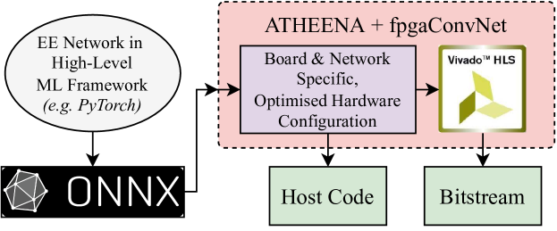
Figure 1: High-level overview of the ATHEENA and fpgaConvNet toolflow.

II Background

Section II-A outlines existing work on input-dependent deep neural network (DNN) computation. We also summarize the well-studied network we use for our experimental study in Section IV-A.

II-A Input-dependent Computation in DNNs

The aim of input-dependent computation is to reduce the computational workload of inference whilst maintaining the accuracy of the network. Static compression methods also reduce computational workload but result in accuracy degradation across all inputs. The introduction of input-dependent, dynamic behaviour customises the computational workload per input, allowing the user to explore the trade-off between accuracy and computational workload. This concept is demonstrated in Dynamically Throttleable Neural Network (TNN) [18]. The network uses a two-stage training approach which first produces a high accuracy network followed by reinforcement learning to train a small DNN module adjacent to the main DNN that has a fine grained control of customizable subsets of the main DNN layers. Similarly, Dynamic Deep Neural Network (D²NN) [19] constructs a network trained with reinforcement learning but has a network topology consisting of ‘regular’ (convolution and fully connected layers) interspersed with ‘control’ nodes which dictate the path a given data sample will take.

An alternative to the architectural freedom of D²NN are the split computing [20] methods. These are located mid-way on a sliding scale of division of computation between edge device and server: at one extreme, there is fully local computation, where inference is performed on an embedded device, and at the other extreme, data is captured and compressed locally [21] before being transmitted via a wireless connection to server for inference. In general, the local computation performs some initial classification (or other ML task) and assesses the confidence of the result. The local compute can then decide whether or not further computation is required and can potentially skip the high latency, round trip of transferring data to power-intensive, server-based compute [22].

Early-Exit networks share structural similarities with split computing and have drawn increasing interest [23] in recent years. The typical architecture of an Early-Exit network is set out in the BranchyNet [16] work and consists of a branching, tree-like structure with a backbone, where the majority of the sample processing is carried out, and exits, which often contain some additional CNN layers and are located at different points along this backbone as illustrated in Figure 2. Due to the hierarchical nature of CNNs [17, 24], the earlier layers in the backbone will have learnt more general or coarser features. As a result, easy samples can be classified based on these features to an acceptable level of accuracy and more complex samples can be further processed in later stages of the backbone before final classification.

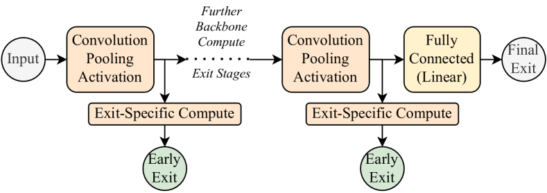
Figure 2: The form of a generic Early-Exit network with backbone stages and varying levels of compute between exits.

The benefit of Early-Exit methods over traditional quantisation and pruning is that the former make use of the varying difficulty of samples within a data set. Reducing precision or removing extraneous parameters common to all samples beyond a certain point will decrease the accuracy of the network over the most challenging samples first. With the implementation of early exits, inference efficiency can be improved beyond these limits. Early-Exit presents a tuneable trade-off between the throughput and accuracy of data samples. The other key benefit of these networks is the improved throughput of batch computation due the average of the reduced latency of early exits and similar latency of later exits. Furthermore, Early-Exit has applications in an array of ML tasks including semantic segmentation [25] and image classification [26, 27].

The ‘difficulty’ of a given data sample is challenging to quantify so there is a range of metrics used in the literature to judge the confidence of a result at a given exit point. A limitation of the deployment of these networks is the resource/latency cost of these exits which may need to compute exponential or logarithmic operations. The most common method of determining confidence is to measure the information entropy [16, 23] of the probability distribution over the available classes. A low entropy value indicates more certainty in the correct result. The other main method to determine confidence is comparing the maximum value in the class probability distribution to a threshold [17]. Both these methods require Softmax computation and the use of logarithmic or exponential functions.

A key challenge in migrating these software-oriented Early-Exit designs to hardware, is to develop an architecture that efficiently executes input-dependent control-flow whilst minimising extraneous computation, area overhead, and maximising the available throughput gains. This is the central challenge we address with ATHEENA in this paper, for the case of Early-Exit networks.

II-B CNN compilers for FPGAs

Taking standard CNNs from software-based inference to accelerated, FPGA-based inference can be accomplished automatically with custom compilers [28]. These broadly fit into two categories: single computation engine architectures and data-flow streaming architectures. The single engine [29] typically consists of a fixed architecture on which the CNN layers are mapped, loaded, and executed in a sequential fashion. The CNN is translated to a list of instructions. This execution can be controlled either by software using CPU or specialised control hardware. The benefit of single engine is that they are amenable to different CNN workloads. However, there is significant benefit, in terms of resource savings and throughput increases, to customising a given architecture to the CNN workload [30]. Streaming architectures take this customizability further by making use of the data-flow paradigm to produce deeply pipelined designs with specialized layers for state-of-the-art CNNs [31].

We adopt the streaming architecture method so that we can benefit from CNN-specific customization and implement the input-dependent compute spatially, targeting high throughput.

II-C fpgaConvNet

fpgaConvNet [32] is an automated CNN-to-FPGA toolflow able to handle common CNN layers and forms a foundation for our toolflow. The streaming architecture used comes from modelling the CNN as a Synchronous Data-Flow Graph (SDFG) [33]. The nodes are the computation operations such as convolution and the arcs are streams of data. This means that the hardware blocks mapping these computations can have a static schedule and compensate for differing data consumption rates with sufficient buffering determined at compile time. Streaming backpressure is handled by the Vivado HLS [34] streaming interface.

fpgaConvNet receives a trained CNN model in the ONNX [2] representation. This device-agnostic representation is parsed to construct the SDFG and populate an initial hardware mapping with templated layers/modules corresponding to the supported ONNX operations (such as convolution and pooling). The tool performs Design Space Exploration (DSE) to optimize the hardware architecture using simulated annealing to select possible incremental transformations to the hardware blocks. This allows an optimized design to be found in a large search space in a relatively short time. Finally, the hardware code is generated in a form suitable for Vivado HLS to compile. The design space exploration makes the most of the flexibility of FPGAs. It makes use of resource models of the hardware blocks as well as the target board resources and the model of the mapped CNN workload. The toolflow is also able to accommodate different application objectives since it is possible to optimize the design for latency or throughput.

For larger CNNs, folding is used to tune the amount of intermediate computation required to compute a full result. Folding the inputs and intermediate feature maps multiplexes sections of the design in time to reduce resource consumption. This is accomplished at two scales: coarse-grain folding at the input and output of layers and fine-grain folding of the sliding windows within the convolution module.

fpgaConvNet was chosen as a basis for our work because of the existing hardware templates for fundamental CNN layers and the tooling infrastructure that provides DSE to generate a network layer configuration for hardware implementation. fpgaConvNet is open source and demonstrably extensible [35, 36, 37] in a range of contexts. In this work, we transform fpgaConvNet into ATHEENA by extending the scope of supported CNN architectures as well as creating new hardware templates to efficiently support Early-Exit networks. As with existing comparable toolflows [31, 38, 39] (at time of writing), fpgaConvNet does not support the coarse granularity of input-dependent computation of Early-Exit networks. We expand the data-flow model of fpgaConvNet to include input-dependent computation as pipelined control flow. This allows ATHEENA to generate CNN-hardware mappings that benefit from varying data sample difficulty. The method of extension we develop for fpgaConvNet is orthogonal to extreme quantization [39] and exploitation of sparsity [31] detailed in other works. Furthermore, we improve overall compilation times by partitioning the design prior to HLS compilation and automatically stitching generated components prior to synthesis and implementation.

II-D Dynamic Machine Learning on FPGAs

CascadeCNN [40, 41] implements a specialized form of dynamic computation where a runtime decision is made to switch between low and high-precision quantized versions of the same network. The components of the architecture include both a low and high precision implementation of the network on FPGA fabric and the confidence evaluation unit running on a CPU. All data examples are first fed through the low precision network before the computation of a confidence estimate on the results to determine whether the results meet the user-defined accuracy threshold. Any samples with low confidence are fed through the high precision network. ATHEENA is similar in that all data sample processing compute is confined to the FPGA fabric avoiding prohibitive reconfiguration costs [41]. We also choose to include the confidence evaluation on chip for ATHEENA, meaning data does not need to make the round trip to and from off chip memory to perform the confidence decision. The key difference for ATHEENA is the streaming architecture which can achieve higher throughput thanks to deeply pipelined layers.

DynExit [42] uses a hand crafted, single engine architecture to implement a ResNet with classifiers attached along a pre-trained backbone. The network architecture consists of pipelined convolution and linear (fully connected) execution blocks attached to a ‘branch’. The ‘branch’ consists of an exponential and a natural logarithm module to compute the confidence of the classification based on a rearranged version of the cross entropy loss function. Similarly, ATHEENA uses a dedicated block to determine the sample confidence but DynExit lacks customizable layer configurations which limits the accelerator design’s ability to fully utilise the FPGAs resources for different networks.

Adaptive Hierarchical CNN (AHCNN) [43] notes the benefits of being able to utilise the shallow features for easy data sample classification and deeper features of a more accurate network for difficult classifications. To this end, partial reconfiguration is used to swap in and out shallow and deeper sections of a ResNet18 CNN. Large batch sizes are used to amortise the latency penalty for reconfiguration. This allows the design to benefit from full utilization of the resources for each stage of network computation but the latency penalty is prohibitive for low latency applications. They also compute the confidence decision based on the maximum value of the Softmax, as with ATHEENA, but couple this with the profiled probability of the occurrence of a given class. This equates to a confidence threshold that is class-dependent.

The heterogeneous architecture proposed in [44] makes use of the FPGA fabric to accelerate the highly parallel CNN computation through the use of multiple processing elements in a systolic array architecture. The onboard CPU computes the Softmax and entropy of the intermediate classification results. As with DynExit, this is another hand-crafted architecture that supports the main convolution kernel sizes but currently has limited support for more recent networks.

Interest is growing in the use of input-dependent computation, however, none of these works provide a fully automated toolflow for mapping Early-Exit CNNs to FPGAs. It is this problem we tackle in this paper.

III Methodology

The fundamental issue of implementing Early-Exit networks on FPGAs is determining a hardware mapping that balances the control and data-flow throughput requirements whilst minimising latency overhead. A naive implementation would have all stages of the network optimized for the highest possible throughput. However, in the presence of any resource constraints this is clearly a sub-optimal strategy: having all stages targeting the same fixed throughput will lead to some stages being under-resourced bottlenecks and others being starved of data samples. Hence in this work we target the following problem: given an FPGA platform with certain computational and memory resources, what is the best way to allocate those resources to maximise throughput for a given expected distribution of samples of varying difficulty. We first define our methodology for determining this optimized resource allocation for Early-Exit networks, and then explain the detail of the toolflow and template hardware designs we introduce to fpgaConvNet for ATHEENA. The code will be open-sourced.

III-A Scaling Resource Allocation according to Exit Probability

Early-Exit networks can be divided into sections according to the stages of compute between each exit. For ease of presentation, we explain the area apportioning process with reference to a two-stage network, however it is trivial to extend the presentation to multi-stage networks. We illustrate the methodology with the generic, two-stage network in Figure 3 before applying it to BranchyNet in Section IV-A. The network is first separated into two stages at the layer level. This means dividing the network into the first stage, containing all the parts of the backbone and the Early-Exit layers that are need to operate at the higher data rate, and the second stage containing the remaining parts of the backbone and final exit. This second stage is only required to operate at a lower data rate because not all input data samples pass through this hardware. As a result, network classification decisions may also return out-of-order. The key challenge is to automate the design of a hardware architecture capable of efficiently supporting these multiple data rates. To this end, we can use existing FPGA design tools capable of folding (in our case fpgaConvNet) to generate separate, optimized Throughput-Area Pareto (TAP) functions for both stages which we then merge to generate a combined TAP function as visualized in Figure 4.

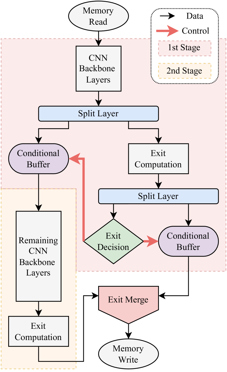
Figure 3: High-level diagram of the proposed control-flow hardware attached to the CNN layers of fpgaConvNet for a two stage network. Black arrows represent normal data-flow plus Sample ID tags and red arrows represent control signals.

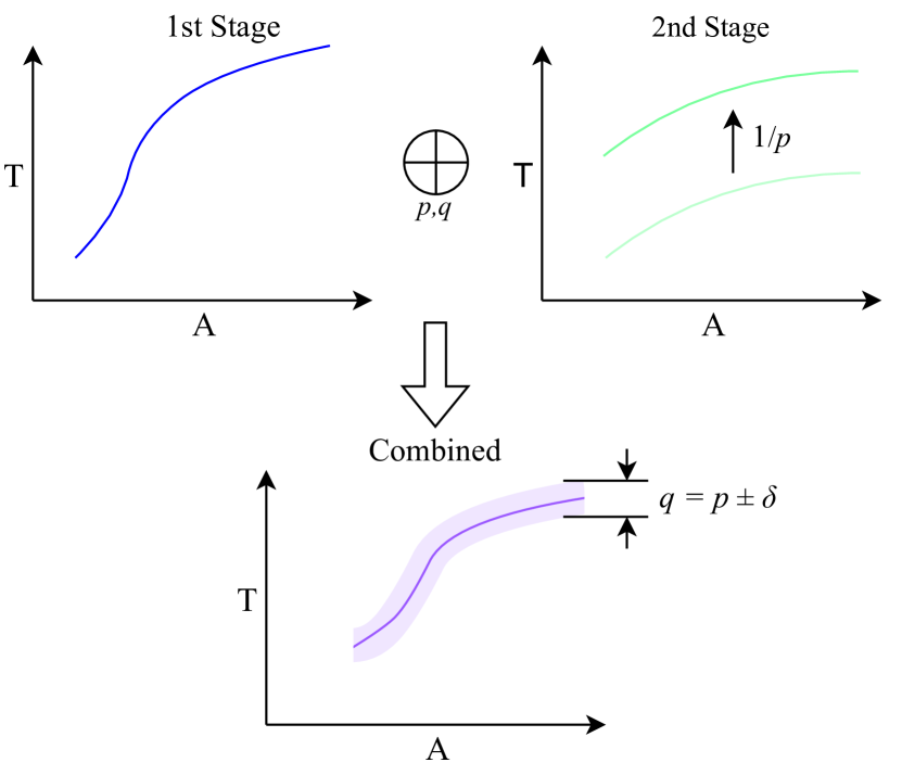
Figure 4: Visual representation of the scaling and combination of TAP curves for network stages. Our process combines two TAP graphs with respect to an expected probability $p$. This $p$ corresponds to the percentage of samples that require processing by second stage. $q$ denotes throughput deviations from this design-time probability that may be encountered at runtime.

We define a TAP function as a function that is (non-strictly) monotonically increasing in each of its arguments. The principle is that this function captures the maximum achievable throughput possible by separately optimizing a section of the network for a given fraction of total resources. Let $\mathbb{N}$ denote the set of natural numbers and $\mathbb{Q}$ denote the set of rational numbers. An example of a TAP function might then be, $f:\mathbb{N}^{4}\to\mathbb{Q}$, capturing the optimal throughput possible with a constrained number of BlockRAMs, DSPs, FFs, and LUTs, as represented by the four arguments to the function. A function like this is automatically generated by providing the fpgaConvNet optimizer limited fractions of the board resource constraints. The results for each set of constraints are collated for input to the ATHEENA optimizer. The 1st Stage and 2nd Stage graphs of Figure 4 show a sketch of some TAP functions for the first and second stage of a two-stage network.

Our objective is to combine these two TAPs into a single TAP for the Early-Exit network. We may think about the problem in this way: since the second stage is only expected to be used by each input sample with some probability $p\in(0,1]$, it follows that, given suitable buffering between stages, it is possible to extract a higher throughput than the nominal throughput of the design, by a factor $1/p$.

The overall design will be limited by the throughput of the first stage or the second stage scaled by $1/p$, whichever is lower. However, in any practical setting, the probability for an input sample to need further processing by the second stage will differ by some degree from the (profile-based) probability for which the hardware was designed. We therefore denote the design-time probability estimate as $p$ and the actually encountered probability as $q$. Putting these components together, we are able to define an ideal combination of the two TAPs, parameterised by $p$ and $q$, expressed formally below, and illustrated in Figure 1 where $\oplus$ denotes the so-defined TAP combination operator.

$$f\underset{p,q}{\oplus}g:x\mapsto\min(f(x_{1}),g(x_{2})/q)$$ (1)

$$\mathrm{where}\;(x_{1},x_{2})=\underset{\underset{\textrm{ s.t. }x=x_{1}+x_{2}}{x_{1},x_{2}}}{\arg\max}\min(f(x_{1}),g(x_{2})/p)$$

Intuitively, what this equation tells us is that for a given total resource budget $x$, we should apportion a resource allocation $x_{1}$ for the first stage and $x_{2}$ for the second stage maximising the throughput of the limiting stage, taking into account our design-time estimate of probability $p$. At runtime, the throughput demand on the first stage will be as expected, but may vary somewhat from the design-time expectation on the second stage. This is all illustrated in the lower plot of Figure 4. The design points represented by the TAP function for the first and second stages are discrete. This means that it is unlikely for the tool to be able to perfectly match the predicted throughput values. In the case that the second stage is the limiting factor, a reduction in the use of this stage, corresponding to $q<p$, will result in an increase in throughput. For $q>p$, the throughput will be reduced due to the reliance on the limiting stage. These situations are represented by the shaded region. The solid purple line corresponds to $q=p$ , in which the probability of hard samples matches that of the profiled, design-time probability.

The following section explains how we obtain our probability profiles and use them to inform the combination of TAP functions in the manner previously described. ATHEENA builds on fpgaConvNet and automates this process for the user. We demonstrate this process in practice in Section IV.

III-B Toolflow Extensions & Automation

We build the ATHEENA toolflow by extending the open-source fpgaConvNet as illustrated in Figure 5. The fundamental difference between the flows is that the original fpgaConvNet constructed a data-flow graph whereas we require a control and data-flow graph (CDFG) to represent the flow of data through layers as well as the confidence decisions at the end of the early exits. Modifications to the parser and optimizer are made to support the different ONNX operations and encompass the control-flow for hardware translation. Several new hardware component templates (detailed in Section III-C) are designed for the FPGA implementation of control-flow and to support the confidence calculation.

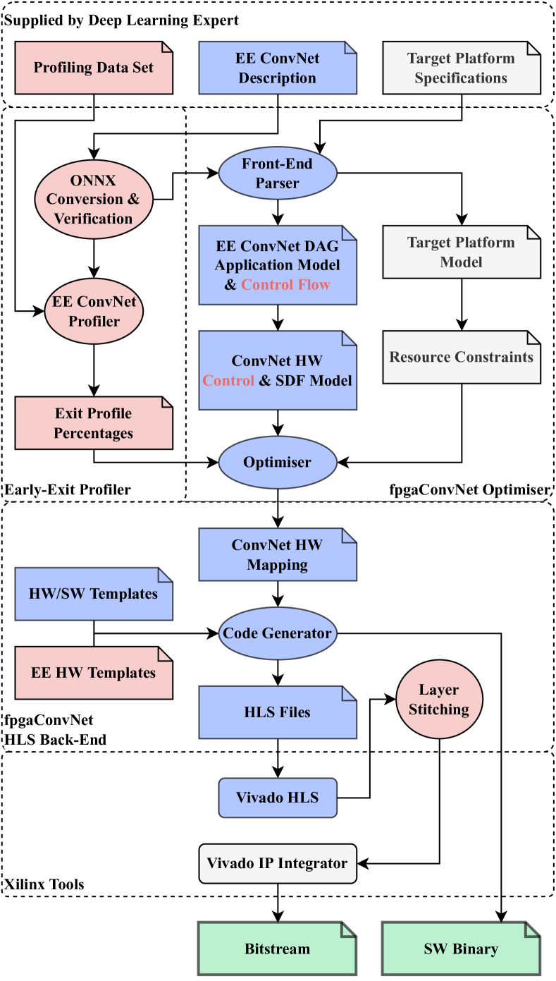
Figure 5: A visual representation of the ATHEENA toolflow. We have built upon the baseline, open source fpgaConvNet toolflow. New elements are in red and modified elements are in blue.

III-B1 Early-Exit Profiler

We introduce the Early-Exit profiler which takes a profiling data set and the high-level Early-Exit ConvNet description and apportions the set so that multiple distinct tests can be run which will have a similar probability of hard samples on average but variation individually. Batched inference is performed over the sets followed by collection of the exit probabilities, exit accuracy, and cumulative accuracy. The average probability of hard samples is fed into the optimizer as $p$, along with the multi-stage CDFG hardware model. The ATHEENA optimizer then creates an optimized mapping for the different stages of the network, scaling resource constraints according to $1/p$.

III-B2 HLS Limitations & Parallel Compilation

In order to allow for HLS-based compilation of large networks, we automatically split the network into the individual layers, generating top-level HLS files for each. This results in multiple smaller designs for HLS that can be compiled independently. The layers are then automatically stitched together at the board design stage in Vivado IP Integrator in conjunction with the supporting processor and memory interfaces. A DMA controller is introduced with input and output FIFOs to manage the transfer of data between the host and the FPGA. Since the Early-Exit board design now consists of multiple HLS cores, they each need a start signal from the host CPU. These signals are automatically added into the host code, in addition to the DMA read and write transfers set to batch size specified by the user. By the end of the compilation, the user has a bitstream and complementary host code to perform batch inference on the board.

III-B3 ONNX Conversion

We make some minor modifications to the benchmark source code so that it can be converted into a compatible ONNX form using our Early-Exit profiler. As the original networks were typically run in software, PyTorch (version 1.8.1) handles the scheduling of the network graph execution for CPU and GPU inference. ONNX generation from a PyTorch description of simple network is trivial but the inclusion of conditional operations requires the PyTorch description to explicitly prevent the operations from being removed by software optimization passes. These network control-flow decisions need to be captured and translated to FPGA-based hardware blocks. We use the PyTorch scripting methods as an intermediate stage [45]. This converts the network into a PyTorch-specific intermediate representation capable of supporting conditional statements. PyTorch-based ONNX methods then convert the intermediate representation to the final ONNX form. An inference test is performed with the ONNX form and the results compared to the original to verify the conditional functionality matches that of the PyTorch implementation.

III-C Early-Exit Network Layers: Hardware Templates

We extended the ONNX parser of fpgaConvNet to support the operations required by the Early-Exit CNNs. These operations include:

• Softmax

• Reduction (ReduceMax)

• Numerical comparison (Greater than)

• If conditional

Figure 6 illustrates the new Early-Exit layer templates and Figure 3 provides a high-level view of the proposed placement of these layers within the pre-existing CNN data-flow operations in fpgaConvNet.

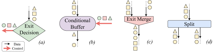
Figure 6: Newly added Early-Exit Hardware layer templates. The shapes represent a given Sample ID. For the Conditional Buffer and Exit Decision, we have indicated whether the Sample ID is kept (green) or dropped (red). The associated Sample data is either passed through or dropped. We show that the Exit Merge layer keeps all data for a given Sample ID sequential, opting to stall an exit instead of interleaving.

These operations are the foundation of the conditional aspect of the network so are merged into one hardware layer comprising of distinct modules. The remaining layers added do not correspond to ONNX operations but support the control flow extensions of the SDF paradigm. The newly added layers match the fixed-point representation with the exception of the Exit Decision layer. This instead uses single-precision floating-point as this preserves the numerical behaviour of the exponential function at its core.

III-C1 Exit (Softmax) Decision Layer

An early exit will occur if Condition (2) holds for some threshold $C_{thr}$ determined after training prior to exit profiling, where the standard $\textrm{Softmax}:\mathbb{R}^{C}\to\mathbb{R}^{C}$ function corresponds to (3), used to transform the vector of class activations into a probability distribution, where exponentiation of vectors is interpreted component-wise [24].

$$\max_{i\in\{1\ldots C\}}\left[\textrm{Softmax}(x)\right]_{i}>C_{thr}$$ (2)

$$\textrm{Softmax}(x)=\frac{\exp(x)}{\sum^{C}_{j=1}\exp(x_{j})}$$ (3)

$C$ is the number of classes, $x_{i}$ is the network output for the $i$th class, and $C_{thr}$ is the confidence threshold.

This layer, along with the exit-specific computation required for the Early-Exit classifier dictate the minimum size of buffering required between the intermediate result and the conditional buffer layer to prevent a pipeline stall (Figure 7). On a small FPGA this has the potential to be a prohibitively large amount of memory required so the need to reduce the latency of the operation is key to the implementation of Early-Exit networks.

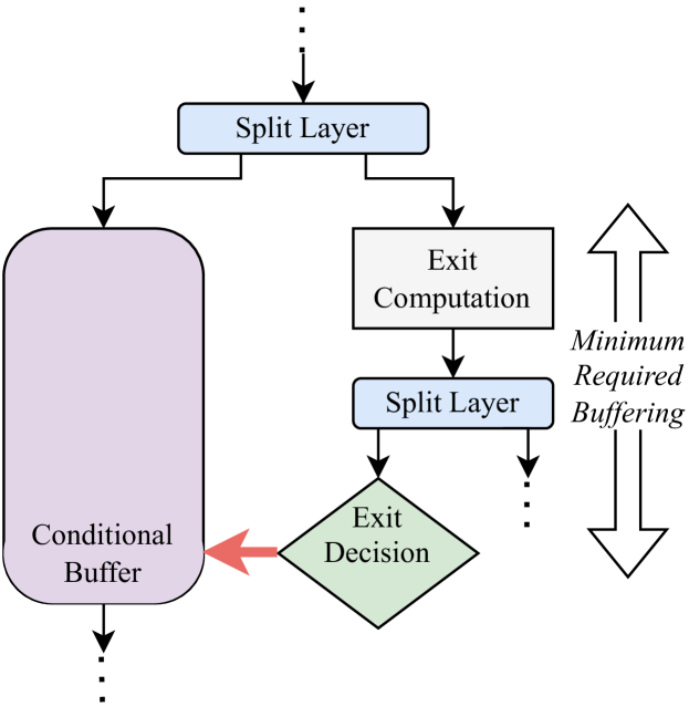
Figure 7: The latency of the additional exit computation and exit decision layers is used to determine the minimum amount of buffering required by the conditional buffer to prevent deadlock in the design.

The operation can be rearranged to remove the division as in (4) to decrease the resource overhead and latency of the decision component. The use of floating-point for this layer means that addition and comparison operations incur a significant latency penalty given a target frequency. To reduce this penalty, we implement adder and comparison trees to compute results in parallel, minimising the latency of this layer.

$$\max_{i\in\{1\ldots C\}}\exp(x_{i})>C_{thr}\cdot\sum^{C}_{j=1}\exp(x_{j})$$ (4)

III-C2 Conditional Buffer Layer

Two challenges arise from the addition of control flow from conditional buffers. The first challenge is that, after the first stage of the network, data samples will go down the path to the early exit or the path to the second stage. Let’s assume $N$ data samples, $K$ will exit early while $N-K$ will continue through the second stage. The existing fpgaConvNet hardware layers in the second stage expect $N$ data samples and the implementation of the pipeline will only terminate on the final $N$th data sample. To avoid deadlock, we flush the pipeline with an unused sample ID and corresponding data.

The second challenge is that there is a significant amount of computation between the point at which the network first has to buffer data and the point at which control signals are produced. We temporarily buffer the unfinished data sample while the confidence metric is evaluated as well as the fully processed sample result at the early exit classification stage. If the sample can exit early, the buffer drops the intermediate data and the classification result of the early exit is transferred to memory via the exit merge component. Due to the size of the intermediate feature map buffer, it is important to reduce the impact of both reading in and writing out of the buffer (effectively doubling the latency of the layer for every sample prior to the control signals). To drop an unused feature map we invalidate the addresses of the stored feature map in a single cycle. If the sample cannot exit, the buffer passes the intermediate data through to the next stage of the backbone. The fundamental operation of the conditional buffer is to filter the easy samples from the hard samples. The buffer prevents the later stages of the backbone from unnecessary computation, which has the effect of increasing throughput because of the lower expected data rate for the second stage. This component will be included in the open-source repository.

III-C3 Split Layer

The split layer is used to duplicate the result of layers at the branching points in the Early-Exit network. This splits the data-flow stream to allow a copy of the data to continue down the backbone in parallel to the early exit layers.

III-C4 Exit Merge Layer

Inference is run on a batch of data samples where each data sample consists of a fixed number of pixels. In line with other static streaming architectures, the original fpgaConvNet has no built-in distinction between data samples in the pipelined hardware. Each component will continue to operate on newly provided pixels and the user is responsible for interpreting the results based on their location in memory. However, given that in an Early-Exit network, data samples within a batch are able to complete out of order, there needs to be an internal representation of each data sample’s position within the batch. A Sample ID is assigned to each data sample and is passed through the hardware with each pixel. At the conditional buffers, the IDs are compared to determine whether or not to drop the data points with a given ID. When a sample exits the network, the exit selection layer coherently merges the exit streams into one memory writing component. This may result in the stalling of one network path while another is allowed to pass through.

IV Experimental Results

The following section details a case study of using the ATHEENA toolflow to automatically implement the previously-proposed Branchy-LeNet network [16] directly from PyTorch code. This starts with some minor modifications to the source architecture shown in Figure 8. The network was trained and tested in the manner outlined in the original paper. The alterations resulted in a negligible change in accuracy and a similar Early-Exit probability for a comparable $C_{thr}$ value in software. These modifications reduce wasted compute on the board and improve compatibility with standard fpgaConvNet convolution layers. The Early-Exit profiler is used to generate the ONNX representation and Early-Exit probabilities for the extended fpgaConvNet optimizer. This in turn creates a hardware mapping for the Early-Exit and fpgaConvNet layers for the chosen board. The tool then converts the mapping into HLS code and compiles the layers in parallel before stitching them together and generating a bitstream with associated host code.

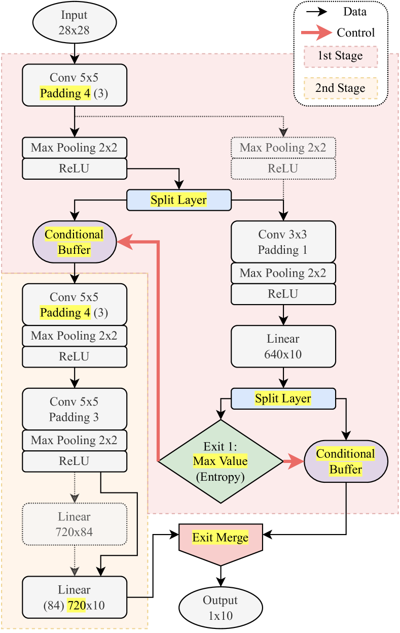
Figure 8: Slightly modified version of B-LeNet [16] for fpgaConvNet. Changes are highlighted in yellow with original values in brackets. Faded layers have been removed from the architecture. Hardware-only layers (detailed in Section III-C) have been added.

(a) Throughput Area results generated by the simulated annealing optimizer stage of the toolflow at a $p$ of 25% and $q=p\pm 5\%$.

(b) Throughput Area results obtained using ZC706 board. At a $p$ of 25%. Tested using data sets consisting of $q=30\%,25\%,20\%$.

Figure 9: The red line represents the corresponding baseline results for fpgaConvNet and the limiting resources for each point are denoted by the following: (BRAM), (LUT), (DSP). Designs A1, A2, A3, and B1, B2, B3 have detailed resource usage in Table I.

IV-A BranchyNet: Hardware Experimental Study

The experimental setup follows that of fpgaConvNet to make comparison direct and expedite the gathering of results. The target device is the Xilinx ZC706 board [46] with the Zynq 7045 System on Chip (SoC). The resources available are 218600 LUTs, 437200 FFs, 900 DSPs, and 1090 18K BRAMs. Vivado HLS 2019.1 was used for compatibility with fpgaConvNet. Each design is conservatively clocked at 125MHz (limited by HLS and board). We compare our hardware Early-Exit implementation to a corresponding single-stage network baseline. This single-stage (backbone) consists of the network layers from the start of the Early-Exit network through to the end of the second stage. For BranchyNet, this means three Convolution, Pooling and ReLU layers followed by a Linear (Fully Connected) layer.

Both the ATHEENA optimizer and baseline optimizer are provided the board resources constrained at different percentages in order to generate a Throughput-Area Pareto curve. Due to the random aspect of the simulated annealing within both optimizers, they are run ten times and the best points are chosen to form the curve. Additionally, a range of data points with constrained resources allows us to infer throughput gains/resource savings on boards with lower available resources. Once the optimizers generate the hardware mapping, we collate the predicted results shown in Figure 9(a) and then pass through the best performing subset of these results to the HLS backend in order to generate the board design. Figure 9(b) shows the resulting Throughput-Area Pareto curve after synthesis, implementation and place-and-route. The resource usage is recorded and the board loaded with each bitstream. The automatically generated host code for the board loads a batch of 1024 samples onto off-chip memory and enables the DMA transfers to and from the design. We measure the total time taken from the start of the DMA transfer until the DMA block registers as being idle and use this to calculate the throughput of the network. The same DMA controller is present for baseline and Early-Exit implementations so the impact on resources is consistent for a fair comparison.

The baseline results are represented by the red lines in Figure 9. While the fpgaConvNet model is not accurate on a point by point basis, the trend is consistent for the predicted and board implementations. To allow for a fair comparison, we included an implemented point predicted by the optimizer to consume greater than the boards resources, in practice the design point B3 consumed $98\%$ of the DSPs. For higher resource allowances, we can see that the designs tend towards being limited by DSPs, this is due to the baseline optimizer selecting an increased level of parallelism for the Convolution and Linear layers and is common to both the baseline and ATHEENA board implementations.

The solid purple line shows the case when the $q$ (percentage of easy samples in the test set) matches that of $p$ (the profiling data set percentage), in this case a $q=p=25\%$. The dashed lines represent a range of points taken on the Throughput-Area space with a differing percentage of hard samples. The predicted results are calculated under ideal conditions: assuming a regular sequence of easy and hard samples and sufficient buffering such that second network stage is able to achieve the estimated throughput.

For the implemented board results, we sample a batch from the test data set for the task. The sampled test set has a split of easy and hard samples proportioned according to the required test probabilities but distributed randomly within the batch of 1024 samples. The lower dashed line represents a $q=30\%$ and demonstrates a partially reduced throughput for some of the data points. The upper dashed line represents a $q=20\%$ and shows that some sub-optimal profiling situations can still result in throughput increase thanks to the significant latency reduction of data samples exiting at the high-throughput first stage. The results demonstrate the potential for greatly improved throughput at the risk of slightly decreased throughput caused by differences between test and profiling exit probabilities, and variation in exit distribution within a batch. Additionally, the predicted Throughput-Area curve is a good approximation of the measured implementation results. We can see the ATHEENA model is slightly optimistic in terms of achievable throughput. This is likely due to sub-optimal resource models for the new components and the variability of HLS compilation. Finally, the gap between lower dashed line and the baseline is indicative of the robustness of the approach to the difference between $p$ and $q$ for a real world application, assuming sufficiently sized buffers.

TABLE I: Tabulated resource comparison for implemented Baseline Vs ATHEENA on ZC706 board. *Maximum limiting resource.

	LUT	FF	DSP	BRAM	Limiting Resource (%)	Throughput (Samples/s)
B1	75513*	61361	295	55	35	13513
A1	68383*	63170	169	206	31	19434
B2	105451	84761	470*	89	52	21276
A2	128940*	117138	407	239	59	47583
B3	138194	120764	885*	170	98	43384
A3	163637	142913	742*	265	82	94170

TABLE II: Resource overhead of the Early-Exit for labelled designs compared to the network backbone. This includes the resource usage attributed to the additional Early-Exit computation and buffering required for operation of B-LeNet. The proportion of this overhead is detailed as a percentage of the total design.

	LUT	%	FF	%	DSP	%	BRAM	%
A1	13912	20	13595	22	34	20	114	55
A2	37766	29	35941	31	122	30	146	61
A3	33166	20	30974	22	112	15	186	70

The maximum measured ATHEENA throughput is $2.17\times$ the the maximum measured baseline throughput. ATHEENA achieves this throughput using 16% fewer DSPs (the limiting resource) when the resources are apportioned between the first and second stage according to the profiled probabilities. Alternatively, ATHEENA can achieve the same throughput as the maximum baseline using $46\%$ of the design’s limiting resource.

The design points in Table I show that the achieved throughput increase comes at the cost of an increase in BRAM. The designs A1, A2, and A3 (labelled in Figure 9(b)) require this as part of the conditional buffers to store enough of intermediate feature map samples to prevent deadlock, as there is a delay from the point the buffered data and the related control signal are produced. Furthermore, additional BRAM is added to increase robustness to variation in the hard samples’ exit probability. This results in the resource overhead from implementing the additional classifier layers, comparison layer, and conditional buffering layers being dominated by BRAM usage, as detailed in Table II with design A3 having $70\%$ of the total BRAM usage within the early exit overhead.

The predicted throughput of each stage of the Early-Exit network is calculated separately. The resulting design points for each stage form a discrete Pareto front. When the optimizer is selecting from these two stages and scaling the throughput of the second stage, there will often be a discrepancy between the predicted throughputs of the stages. If the resulting combined design point over-provisions the second stage then the design will be more robust to variations in the testing data set probability. Excluding the BRAM usage, we can see that the Early-Exit resource overhead is higher for design point A2, suggesting that the throughput is more tightly coupled to the performance of the first stage of the network.

TABLE III: Comparison against BranchyNet reported accuracy, converted throughput and converted hard sample probability.

Network		Top 1 Acc. (%)	$p$ (%)	Throughput (Sample/s)
CPU	LeNet	99.20	-	297
CPU	B-LeNet	99.25	5.7	1613
GPU	LeNet	99.20	-	633
GPU	B-LeNet	99.25	5.7	2941
Baseline	LeNet	98.84	-	43384
ATHEENA	B-LeNet	98.88	25.0	94170

The original BranchyNet paper details an implementation of the LeNet and Branchy (B) LeNet networks using using a 3.0GHz CPU with 20MB L3 Cache and NVIDIA GeForce GTX TITAN X (Maxwell) 12GB GPU. They report the average latency of a single sample in milliseconds. We convert their per sample average latency metric into a throughput metric for the comparison in Table III. Both our baseline and ATHEENA designs benefit from adaptations of the network architecture to be more amenable to a hardware implementation. These changes include quantisation to a fixed-point representation, adjusting layer parameters, and adapting the exit condition computation. This has a marginal effect on the accuracy compared to the software implementations and is partly the reason for such high gains compared the CPU and GPU implementations. We are able to exploit per-sample parallelism more effectively using the streaming architecture however the relative gains of implementing Early-Exit on CPUs and GPUs is greater than demonstrated by our toolflow in part due to necessary reduction of exit percentage to maintain accuracy. Despite this, we find that a $p=50\%$ still results in a throughput improvement relative to the baseline in spite of the area overhead for the additional layers and control logic embedded in the Early-Exit streaming architecture. Overall, significant gains in throughput can be achieved from utilising an optimized streaming architecture converting a CNN implementation to FPGAs and up to $2.17\times$ further gains from implementing customised Early-Exit hardware tailored to the design.

IV-B Benchmarking Results

We include an additional two networks in Table IV. The best performing predicted throughput and corresponding resource results have been taken from the optimizer stage of the baseline and ATHEENA toolflows. Due to the increased size of these networks we specify the target platform as the Xilinx VU440. We use the percentage of hard samples outlined in the papers to generate the two-stage design. We have included software-based implementations of these networks in the open source repository.

TABLE IV: Resulting throughput improvement for two-stage accelerator designs generated by ATHEENA model compared to fpgaConvNet baseline. *Implemented on Xilinx ZC706

Network	Toolflow	Limiting Resource		$p$	Throughput
(Task)		Type	%	(%)	(Samples/s) Gain
B-LeNet[16]	Baseline*	DSP	84	-	43384     1.00$\times$
(MNIST)	ATHEENA*	DSP	88	25	94170     2.17$\times$
Triple Wins[27]	Baseline	DSP	86	-	19524     1.00$\times$
(MNIST)	ATHEENA	DSP	81	25	54220     2.78$\times$
B-AlexNet[16]	Baseline	DSP	84	-	8676     1.00$\times$
(CIFAR10)	ATHEENA	DSP	88	34	17357     2.00$\times$

V Conclusions

We have demonstrated the benefits of the input-dependent computation paradigm in improving CNN mapping to FPGAs by developing a toolflow that allows for the exploration of the throughput-area trade-off space of Early-Exit network hardware implementations orthogonal to benefits from quantisation and pruning employed by other frameworks. We have proposed an approach to automate the production of Early-Exit networks based on a probabilistic proportioning of resources between parts of the computation operating at different data rates, and expanding an existing toolflow. This is achieved with development of specific Early-Exit layers that can handle the intermediate buffering and conditional data-flow requirements of these networks. We verify the toolflow’s model of predicted performance by implementing multiple, resource-constrained, designs points on an FPGA board with randomised test samples. The robustness of the approach is explored using adapted test sets with known Early-Exit probability variation. The resulting ATHEENA framework can transform high-level Early-Exit CNNs into optimized FPGA hardware that out perform their standard CNN counterparts in terms of throughput for a given board or area constraint.

References

- [1] A. Krizhevsky, I. Sutskever, and G. E. Hinton, “Imagenet classification with deep convolutional neural networks,” in Proceedings of the 25th International Conference on Neural Information Processing Systems - Volume 1, ser. NIPS’12. Red Hook, NY, USA: Curran Associates Inc., 2012, p. 1097–1105.
- [2] Facebook, “Open neural network exchange,” 2017. [Online]. Available: https://onnx.ai/
- [3] E. Wang, J. J. Davis, R. Zhao, H.-C. Ng, X. Niu, W. Luk, P. Y. K. Cheung, and G. A. Constantinides, “Deep neural network approximation for custom hardware: Where we’ve been, where we’re going,” ACM Comput. Surv., vol. 52, no. 2, may 2019. [Online]. Available: https://doi.org/10.1145/3309551
- [4] P. Molchanov, S. Tyree, T. Karras, T. Aila, and J. Kautz, “Pruning convolutional neural networks for resource efficient inference,” in 5th International Conference on Learning Representations, ICLR 2017, Toulon, France, April 24-26, 2017, Conference Track Proceedings. OpenReview.net, 2017. [Online]. Available: https://openreview.net/forum?id=SJGCiw5gl
- [5] S. Han, J. Kang, H. Mao, Y. Hu, X. Li, Y. Li, D. Xie, H. Luo, S. Yao, Y. Wang, H. Yang, and W. J. Dally, “ESE: efficient speech recognition engine with compressed LSTM on FPGA,” CoRR, vol. abs/1612.00694, 2016. [Online]. Available: http://arxiv.org/abs/1612.00694
- [6] M. van Baalen, C. Louizos, M. Nagel, R. A. Amjad, Y. Wang, T. Blankevoort, and M. Welling, “Bayesian bits: Unifying quantization and pruning,” in 34th Conference on Neural Information Processing Systems (NeurIPS 2020), 2020.
- [7] R. Abra, D. Denisenko, R. Allen, T. Vanderhoek, S. Wolstencroft, and M. Gibson, “Low precision networks for efficient inference on fpgas,” in 2021 International Conference on Field-Programmable Technology (ICFPT), 2021, pp. 1–5.
- [8] D. Lee, S. J. Kwon, B. Kim, Y. Jeon, B. Park, and J. Yun, “Flexor: Trainable fractional quantisation,” in 34th Conference on Neural Information Processing Systems (NeurIPS 2020), 2020.
- [9] Y. Umuroglu, N. J. Fraser, G. Gambardella, M. Blott, P. Leong, M. Jahre, and K. Vissers, “Finn,” Proceedings of the 2017 ACM/SIGDA International Symposium on Field-Programmable Gate Arrays, 2 2017. [Online]. Available: http://dx.doi.org/10.1145/3020078.3021744
- [10] Z. Lin, M. Courbariaux, R. Memisevic, and Y. Bengio, “Neural networks with few multiplications,” in 4th International Conference on Learning Representations, ICLR 2016, San Juan, Puerto Rico, May 2-4, 2016, Conference Track Proceedings, Y. Bengio and Y. LeCun, Eds., 2016. [Online]. Available: http://arxiv.org/abs/1510.03009
- [11] E. H. Lee, D. Miyashita, E. Chai, B. Murmann, and S. S. Wong, “LogNet: Energy-Efficient Neural Networks Using Logarithmic Computation,” in 2017 IEEE International Conference on Acoustics, Speech and Signal Processing (ICASSP), 2017, pp. 5900–5904.
- [12] J. Ba and R. Caruana, “Do deep nets really need to be deep?” in Advances in Neural Information Processing Systems, Z. Ghahramani, M. Welling, C. Cortes, N. Lawrence, and K. Q. Weinberger, Eds., vol. 27. Curran Associates, Inc., 2014.
- [13] M. Sandler, A. Howard, M. Zhu, A. Zhmoginov, and L. Chen, “Mobilenetv2: Inverted residuals and linear bottlenecks,” in 2018 IEEE/CVF Conference on Computer Vision and Pattern Recognition, 2018, pp. 4510–4520.
- [14] M. Tan and Q. V. Le, “Efficientnet: Rethinking model scaling for convolutional neural networks,” in Proceedings of the 36th International Conference on Machine Learning, ICML 2019, 9-15 June 2019, Long Beach, California, USA, ser. Proceedings of Machine Learning Research, K. Chaudhuri and R. Salakhutdinov, Eds., vol. 97. PMLR, 2019, pp. 6105–6114. [Online]. Available: http://proceedings.mlr.press/v97/tan19a.html
- [15] J. Lin, W. Chen, Y. Lin, J. Cohn, C. Gan, and S. Han, “Mcunet: Tiny deep learning on iot devices,” in 34th Conference on Neural Information Processing Systems (NeurIPS 2020), 2020.
- [16] S. Teerapittayanon, B. McDanel, and H. T. Kung, “Branchynet: Fast inference via early exiting from deep neural networks,” in 23rd International Conference on Pattern Recognition, ICPR 2016, Cancún, Mexico, December 4-8, 2016. IEEE, 2016, pp. 2464–2469. [Online]. Available: https://doi.org/10.1109/ICPR.2016.7900006
- [17] G. Huang, D. Chen, T. Li, F. Wu, L. van der Maaten, and K. Q. Weinberger, “Multi-scale dense networks for resource efficient image classification,” in 6th International Conference on Learning Representations, ICLR 2018, Vancouver, BC, Canada, April 30 - May 3, 2018, Conference Track Proceedings. OpenReview.net, 2018. [Online]. Available: https://openreview.net/forum?id=Hk2aImxAb
- [18] H. Liu, S. Parajuli, J. Hostetler, S. M. Chai, and B. Bhanu, “Dynamically throttleable neural networks,” Mach. Vis. Appl., vol. 33, no. 4, p. 59, 2022. [Online]. Available: https://doi.org/10.1007/s00138-022-01311-z
- [19] L. Liu and J. Deng, “Dynamic deep neural networks: Optimizing accuracy-efficiency trade-offs by selective execution,” in Association for the Advancement of Artificial Intelligence (AAAI), 2018.
- [20] Y. Matsubara, M. Levorato, and F. Restuccia, “Split computing and early exiting for deep learning applications: Survey and research challenges,” ACM Comput. Surv., vol. 55, no. 5, pp. 90:1–90:30, 2023. [Online]. Available: https://doi.org/10.1145/3527155
- [21] Y. Kang, J. Hauswald, C. Gao, A. Rovinski, T. Mudge, J. Mars, and L. Tang, “Neurosurgeon: Collaborative intelligence between the cloud and mobile edge,” ACM SIGARCH Computer Architecture News, vol. 45, pp. 615–629, 04 2017.
- [22] C. Lo, Y.-Y. Su, C.-Y. Lee, and S.-C. Chang, “A dynamic deep neural network design for efficient workload allocation in edge computing,” in 2017 IEEE International Conference on Computer Design (ICCD), 2017, pp. 273–280.
- [23] S. Laskaridis, A. Kouris, and N. D. Lane, “Adaptive inference through early-exit networks: Design, challenges and directions,” in Proceedings of the 5th International Workshop on Embedded and Mobile Deep Learning, ser. EMDL’21. New York, NY, USA: Association for Computing Machinery, 2021, p. 1–6. [Online]. Available: https://doi.org/10.1145/3469116.3470012
- [24] I. Goodfellow, Y. Bengio, and A. Courville, Deep Learning. MIT Press, 2016.
- [25] A. Kouris, S. I. Venieris, S. Laskaridis, and N. D. Lane, “Multi-exit semantic segmentation networks,” in Computer Vision - ECCV 2022 - 17th European Conference, Tel Aviv, Israel, October 23-27, 2022, Proceedings, Part XXI, ser. Lecture Notes in Computer Science, S. Avidan, G. J. Brostow, M. Cissé, G. M. Farinella, and T. Hassner, Eds., vol. 13681. Springer, 2022, pp. 330–349. [Online]. Available: https://doi.org/10.1007/978-3-031-19803-8_20
- [26] X. Chen, H. Dai, Y. Li, and X. G. L. Song, “Learning to stop while learning to predict,” in Proceedings of the 37th International Conference on Machine Learning, ser. Proceedings of Machine Learning Research, H. D. III and A. Singh, Eds., vol. 119. PMLR, 7 2020, pp. 1520–1530. [Online]. Available: https://proceedings.mlr.press/v119/chen20c.html
- [27] T. Hu, T. Chen, H. Wang, and Z. Wang, “Triple wins: Boosting accuracy, robustness and efficiency together by enabling input-adaptive inference,” in 8th International Conference on Learning Representations, ICLR 2020, Addis Ababa, Ethiopia, April 26-30, 2020. OpenReview.net, 2020. [Online]. Available: https://openreview.net/forum?id=rJgzzJHtDB
- [28] S. Veneieris, A. Kouris, and C.-S. Bouganis, “Toolflows for mapping convolutional neural networks on fpgas: A survey and future directions,” ACM Computing Surveys, Feb. 2018.
- [29] K. Guo, L. Sui, J. Qiu, J. Yu, J. Wang, S. Yao, S. Han, Y. Wang, and H. Yang, “Angel-eye: A complete design flow for mapping cnn onto embedded fpga,” IEEE Transactions on Computer-Aided Design of Integrated Circuits and Systems, vol. 37, no. 1, pp. 35–47, 2018.
- [30] A. Boutros, E. Nurvitadhi, and V. Betz, “Specializing for efficiency: Customizing ai inference processors on fpgas,” in 2021 International Conference on Microelectronics (ICM), 2021, pp. 62–65.
- [31] M. Hall and V. Betz, “From tensorflow graphs to luts and wires: Automated sparse and physically aware cnn hardware generation,” in International Conference on Field-Programmable Technology, (IC)FPT 2020, Maui, HI, USA, December 9-11, 2020. IEEE, 2020, pp. 56–65. [Online]. Available: https://doi.org/10.1109/ICFPT51103.2020.00017
- [32] S. Veneieris and C.-S. Bouganis, “fpgaconvnet: Mapping regular and irregular convolutional neural networks on fpgas,” IEEE Transactions on Neural Networks and Learning Systems, Feb. 2019.
- [33] E. A. Lee and D. G. Messerschmitt, “Synchronous data flow,” Proceedings of the IEEE, vol. 75, no. 9, pp. 1235–1245, 1987.
- [34] D. Navarro, O. Lucı´a, L. A. Barragán, I. Urriza, and O. Jiménez, “High-level synthesis for accelerating the fpga implementation of computationally demanding control algorithms for power converters,” IEEE Transactions on Industrial Informatics, vol. 9, no. 3, pp. 1371–1379, 2013.
- [35] A. Montgomerie-Corcoran, Z. Yu, and C. Bouganis, “SAMO: optimised mapping of convolutional neural networks to streaming architectures,” in 32nd International Conference on Field-Programmable Logic and Applications, FPL 2022, Belfast, United Kingdom, August 29 - Sept. 2, 2022. IEEE, 2022, pp. 418–424. [Online]. Available: https://doi.org/10.1109/FPL57034.2022.00069
- [36] Z. Yu and C.-S. Bouganis, “Streamsvd: Low-rank approximation and streaming accelerator co-design,” in 2021 International Conference on Field-Programmable Technology (ICFPT), 2021, pp. 1–9.
- [37] A. Montgomerie-Corcoran, S. I. Venieris, and C.-S. Bouganis, “Power-aware fpga mapping of convolutional neural networks,” in 2019 International Conference on Field-Programmable Technology (ICFPT), 2019, pp. 327–330.
- [38] J. Ngadiuba, V. Loncar, M. Pierini, S. Summers, G. D. Guglielmo, J. M. Duarte, P. C. Harris, D. S. Rankin, S. Jindariani, M. Liu, K. Pedro, N. Tran, E. Kreinar, S. Sagear, Z. Wu, and D. Hoang, “Compressing deep neural networks on fpgas to binary and ternary precision with hls4ml,” Mach. Learn. Sci. Technol., vol. 2, no. 1, p. 15001, 2021. [Online]. Available: https://doi.org/10.1088/2632-2153/aba042
- [39] Y. Umuroglu, N. J. Fraser, G. Gambardella, M. Blott, P. H. W. Leong, M. Jahre, and K. A. Vissers, “FINN: A framework for fast, scalable binarized neural network inference,” in Proceedings of the 2017 ACM/SIGDA International Symposium on Field-Programmable Gate Arrays, FPGA 2017, Monterey, CA, USA, February 22-24, 2017, J. W. Greene and J. H. Anderson, Eds. ACM, 2017, pp. 65–74. [Online]. Available: http://dl.acm.org/citation.cfm?id=3021744
- [40] A. Kouris, S. Veneieris, and C.-S. Bouganis, “Cascadecnn: Pushing the performance limits of quantisation in convolutional neural networks,” in 2018 28th International Conference on Field Programmable Logic and Applications (FPL), 2018, pp. 155–1557.
- [41] A. Kouris, S. I. Venieris, and C.-S. Bouganis, “A throughput-latency co-optimised cascade of convolutional neural network classifiers,” in 2020 Design, Automation & Test in Europe Conference & Exhibition (DATE), 2020, pp. 1656–1661.
- [42] M. Wang, J. Mo, J. Lin, Z. Wang, and L. Du, “Dynexit: A dynamic early-exit strategy for deep residual networks,” in 2019 IEEE International Workshop on Signal Processing Systems (SiPS), 2019, pp. 178–183.
- [43] M. Farhadi, M. Ghasemi, and Y. Yang, “A novel design of adaptive and hierarchical convolutional neural networks using partial reconfiguration on fpga,” in 2019 IEEE High Performance Extreme Computing Conference (HPEC), 2019, pp. 1–7.
- [44] D. Paul, J. Singh, and J. Mathew, “Hardware-software co-design approach for deep learning inference,” in 2019 7th International Conference on Smart Computing Communications (ICSCC), 2019, pp. 1–5.
- [45] P. Contributors, “TorchScript Language Reference,” 2019. [Online]. Available: https://pytorch.org/docs/stable/jit_language_reference.html#language-reference
- [46] Xilinx, “ZC706 Evaluation Board,” 2016. [Online]. Available: https://www.xilinx.com/products/boards-and-kits/ek-z7-zc706-g.html#information