Spectral classification of young stars using conditional invertible neural networks

Abstract

Aims. We introduce a new deep learning tool that estimates stellar parameters (such as effective temperature, surface gravity, and extinction) of young low-mass stars by coupling the Phoenix stellar atmosphere model with a conditional invertible neural network (cINN). Our networks allow us to infer the posterior distribution of each stellar parameter from the optical spectrum.

Methods. We discuss cINNs trained on three different Phoenix grids: Settl, NextGen, and Dusty. We evaluate the performance of these cINNs on unlearned Phoenix synthetic spectra and on the spectra of 36 Class III template stars with well-characterised stellar parameters.

Results. We confirm that the cINNs estimate the considered stellar parameters almost perfectly when tested on unlearned Phoenix synthetic spectra. Applying our networks to Class III stars, we find good agreement with deviations of at most 5–10 per cent. The cINNs perform slightly better for earlier-type stars than for later-type stars like late M-type stars, but we conclude that estimations of effective temperature and surface gravity are reliable for all spectral types within the network’s training range.

Conclusions. Our networks are time-efficient tools applicable to large amounts of observations. Among the three networks, we recommend using the cINN trained on the Settl library (Settl-Net), as it provides the best performance across the largest range of temperature and gravity.

1 Introduction

In star-forming regions, it is massive stars that influence the surrounding environment energetically and dynamically during their short lifetime, but the majority of stars formed in star-forming regions are low-mass stars similar to or less than the solar mass. These low-mass stars are not only the most numerous in the star-forming region (Bochanski et al., 2010) but also account for about half of the total stellar mass (Kroupa, 2002; Chabrier, 2003). Living longer than massive stars, these low-mass stars still remain in the pre-main-sequence phase even when the massive stars are dead. These young low-mass stars provide important information for studying stellar evolution and planet formation.

Stellar parameters (e.g. effective temperature, surface gravity, luminosity, etc.) are estimated from photometric or spectroscopic data by various methods. These methods are usually based on characteristic spectral features that vary depending on the type of stars. Therefore, it is important to adopt the appropriate method to the star under consideration and to the observed wavelength range.

As the volume of accumulated observations ever-expand in recent days, it has become important to develop time-efficient tools that analyse large amounts of data in a faster and more consistent way. This is why artificial neural networks (NNs; Goodfellow et al., 2016) have been utilised in many astronomical fields these days. For instance, NNs have been used to predict physical parameters (e.g. Fabbro et al., 2018; Ksoll et al., 2020; Olney et al., 2020; Kang et al., 2022) or to efficiently analyse images such as identifying structures (e.g. Abraham et al., 2018) and exoplanets (e.g. de Beurs et al., 2022) or classifying observations (e.g. Wu et al., 2019; Walmsley et al., 2021; Whitmore et al., 2021). In this study, we develop NNs that can efficiently analyse numerous spectra in the optical wavelength range of young low-mass stars. We prepare our networks to analyse VLT/MUSE observations adopting the wavelength coverage and spectral resolution of MUSE. In the follow-up paper, we will apply our tool to the spectra of young stars in the Carina Nebula observed with VLT/MUSE.

We adopt conditional invertible neural network (cINN) architecture developed by Ardizzone et al. (2021). Estimating physical parameters from observed measurements is a non-trivial task. As the information we obtain from observation is limited due to the information loss during the forward process (i.e. translation from physical systems to observations), different physical systems can be observed similarly or almost identically, which we call a degenerate system. cINN architecture is specialised for solving the inverse problem of the degenerate system (i.e. from observations to physical systems). In particular, cINN has its own advantage in that cINN always provides a full posterior distribution of the physical system without any additional computations. In astronomy, the cINN approach has been used so far to characterise the internal properties of planets (Haldemann et al., 2022), analyse photometric data of young stars (Ksoll et al., 2020), study emission lines in H ii regions (Kang et al., 2022), or infer the merger history of galaxies (Eisert et al., 2023).

The cINN architecture adopts a supervised learning approach that learns the hidden rules from a number of well-labelled data sets of physical parameters and observations. As it is difficult to collect a sufficient number of well-interpreted real observations, synthetic observations have been usually used instead to generate enough training data. In this study, we utilise Phoenix stellar atmosphere libraries (e.g. Allard et al., 2012; Husser et al., 2013; Baraffe et al., 2015) to train cINNs. Selecting Settl, NextGen, and Dusty Phoenix libraries, we introduce three cINNs (Settl-Net, NextGen-Net, and Dusty-Net) trained on each library.

A few studies have developed NNs to analyse low-mass stars from photometric or spectroscopic data (e.g. Ksoll et al., 2020; Olney et al., 2020; Sharma et al., 2020). For example, Ksoll et al. (2020) developed a network using cINN architecture to estimate the physical parameters of individual stars from HST photometric data and Olney et al. (2020) used a convolutional neural network (CNN) to estimate physical parameters (e.g. effective temperature, surface gravity, and metallicity) from near-infrared spectra observed with Apache Point Observatory Galactic Evolution Experiment (APOGEE) spectrograph. Sharma et al. (2020) used CNN as well to diagnose the optical spectra of stars in a wide range of spectral types but their network only estimates the spectral type of the stars, not the other physical parameters. On the other hand, in this paper, our networks directly estimate the stellar parameters from the optical spectrum of low-mass stars, including the stars in both the main sequence and pre-main sequence phases. Moreover, our network provides a posterior distribution by adopting cINN architecture, which is useful to study the degeneracy between parameters.

In this paper, we focus on validating the performance of three cINNs. We evaluate our networks not only on Phoenix synthetic observations but also on real spectra of 36 young low-mass stars to investigate how well our cINNs work on real observations. These stars are template stars in the Class III phase, well-interpreted by literature (e.g. Manara et al., 2013, 2017; Stelzer et al., 2013).

The paper is structured as follows. In Sect. 2, we describe the structure and principles of cINN and explain implementation detail on the machine learning side. In Sect. 3, we introduce our three networks and three training databases. In the following section (Sect. 4), we describe the Class III template stars used in this paper. Our main results are in Sect. 5. We validate our networks using synthetic Phoenix spectra and 36 template stars. We not only evaluate the parameter prediction power of the cINN but also check whether the predicted parameters do explain the input observations. Section 6 present which parts of the spectrum cINN relies mostly upon. In Sect. 7, we investigate the gap between Phoenix synthetic spectra and real observations. We summarise the results in Sect. 8.

2 Neural network

2.1 Conditional invertible neural network

The conditional invertible neural network (cINN; Ardizzone et al., 2019a, b) is a deep learning architecture that is well suited for solving inverse problems that are tasks where the underlying physical properties $\mathbf{x}$ of a system are to be recovered from a set of observable quantities $\mathbf{y}$. In nature, recovering the inverse mapping $\mathbf{x}\leftarrow\mathbf{y}$ is often challenging and subject to degeneracy due to an inherent loss of information in the forward mapping $\mathbf{x}\rightarrow\mathbf{y}$, such that multiple sets of physical properties may appear similar or even entirely the same in observations.

To tackle these difficulties, the cINN approach introduces a set of unobservable, latent variables $\mathbf{z}$ with a known, prescribed prior distribution $P(\mathbf{z})$ to the problem in order to encode the information that is otherwise lost in the forward mapping. The cINN achieves this by learning a mapping $f$ from the physical parameters $\mathbf{x}$ to the latent variables $\mathbf{z}$ conditioned on the observations $\mathbf{y}$, that is

$$f\left(\mathbf{x};\mathbf{c}=\mathbf{y}\right)=\mathbf{z},$$ (1)

capturing all the variance of $\mathbf{x}$ not explained by $\mathbf{y}$ in $\mathbf{z}$, while enforcing that $\mathbf{z}$ follows the prescribed prior $P(\mathbf{z})$. Given a new observation $\mathbf{y}^{\prime}$ at prediction time, the cINN can then query the encoded variance by sampling the latent space according to the known prior distribution and by making use of its invertible architecture run in reverse to estimate the full posterior distribution $p\left(\mathbf{x}|\mathbf{y}^{\prime}\right)$ as

$$p\left(\mathbf{x}|\mathbf{y}^{\prime}\right)\sim g\left(\mathbf{z};c=\mathbf{y}^{\prime}\right),\,\,\mathrm{with}\,\,\mathbf{z}\propto P\left(\mathbf{z}\right),$$ (2)

where $f^{-1}(\cdot,\mathbf{c})=g(\cdot,\mathbf{c})$ represents the inverse of the learned forward mapping for fixed condition $\mathbf{c}$. In practise $P(\mathbf{z})$ is usually prescribed to be a multivariate normal distribution with zero mean and unit covariance, and the dimension of the latent space is chosen to be equal to that of the target parameter space, that is $\dim(\mathbf{z})=\dim(\mathbf{x})$.

The invertibility of the cINN architecture is achieved by chaining so-called (conditional) affine coupling blocks (Dinh et al., 2016). Each of these blocks performs two complementary affine transformations on the halves $\mathbf{u}_{1}$ and $\mathbf{u}_{2}$ of the block input vector $\mathbf{u}$, following

$$\begin{split}\mathbf{v}_{1}&=\mathbf{u}_{1}\odot\exp\left(s_{2}(\mathbf{u}_{2},\mathbf{c})\right)\oplus t_{2}(\mathbf{u}_{2},\mathbf{c})\\ \mathbf{v}_{2}&=\mathbf{u}_{2}\odot\exp\left(s_{1}(\mathbf{v}_{1},\mathbf{c})\right)\oplus t_{1}(\mathbf{v}_{1},\mathbf{c}).\end{split}$$ (3)

As the equation shows, these two transformations are easily inverted given the halves $\mathbf{v}_{1}$, $\mathbf{v}_{2}$ of the output vector $\mathbf{v}$ according to

$$\begin{split}\mathbf{u}_{2}&=\left(\mathbf{v}_{2}\ominus t_{1}(\mathbf{v}_{1},\mathbf{c})\right)\odot\exp\left(-s_{1}(\mathbf{v}_{1},\mathbf{c})\right)\\ \mathbf{u}_{1}&=\left(\mathbf{v}_{1}\ominus t_{2}(\mathbf{u}_{2},\mathbf{c})\right)\odot\exp\left(-s_{2}(\mathbf{u}_{2},\mathbf{c})\right).\end{split}$$ (4)

In both sets of Eqs. (3) and (4), $s_{i}$ and $t_{i}$ ($i\in\{1,2\}$) denote arbitrarily complex transformations, which need not themselves be invertible (as they are only ever evaluated in the forward direction) and can also be learned by the cINN itself when realised as small sub-networks (Ardizzone et al., 2019a, b).

Another advantage of the cINN architecture is that, as the observations are treated as a condition and simply concatenated to the input of the subnetworks $s_{i}$ and $t_{i}$ in each affine coupling layer, it allows for a) an arbitrarily large dimension of the input $\mathbf{y}$ and b) the introduction of a conditioning network $h$ (trained together with the cINN itself), which transforms the input observation into a more helpful, learned representation $\tilde{\mathbf{y}}=h(\mathbf{y})$ for the cINN (Ardizzone et al., 2019b).

2.2 Implementation details

In this paper, we employ a cINN consisting of 11–16 conditional affine coupling layers in the GLOW (Generative Flow; Kingma & Dhariwal, 2018) configuration, where the transformation outputs $s_{i}(\cdot)$ and $t_{i}(\cdot)$ are estimated by a single subnetwork $r_{i}(\cdot)=(s_{i}(\cdot),t_{i}(\cdot))$. The latter choice, reduces the number of sub-networks per affine layer from four to two, reducing network complexity and computation time. As sub-networks $r_{i}$ we employ simple fully-connected architectures consisting of 5–7 layers of size $256$ using the rectified linear unit (ReLU, $\mathrm{ReLU}(x)=\max(0,x)$) as activation function.

The affine coupling layers are, furthermore, alternated with random permutation layers, which randomly (but in a fixed and, thus, invertible way) permute the output vector in between coupling layers to improve the mixing of information between the two streams $\mathrm{u}_{1}$ and $\mathrm{u}_{2}$ (Ardizzone et al., 2019a, b). For the conditioning network $h$, we also employ a three-layer fully-connected architecture with layer size $512$ and ReLU activation, extracting $256$ features in the final layer.

Prior to training, we perform a linear scaling transformation on both the target parameters $\mathbf{x}=\{x_{1},\ldots,x_{N}\}$ and input observations $\mathbf{y}=\{y_{1},\ldots,y_{M}\}$, where each target property $x_{i}$ and input feature $y_{i}$ is modified according to

$$\begin{split}\hat{x}_{i}&=\frac{x_{i}-\mu_{x_{i}}}{\sigma_{x_{i}}},\\ \hat{y}_{i}&=\frac{y_{i}-\mu_{y_{i}}}{\sigma_{y_{i}}},\end{split}$$ (5)

where $\mu_{x_{i}}$, $\mu_{y_{i}}$ and $\sigma_{x_{i}}$, $\sigma_{y_{i}}$, denote the means and standard deviations of the respective parameter/feature across the training data set. These transformations ensure that the distributions of individual target parameters/input features have zero mean and unit standard deviation, and are trivially inverted at prediction time. The transformation coefficients $\mu_{x_{i}}$, $\mu_{y_{i}}$ and $\sigma_{x_{i}}$, $\sigma_{y_{i}}$ are determined from the training set and applied in the same way to new query data.

We train the cINN approach for this problem by minimisation of the maximum likelihood loss as described in (Ardizzone et al., 2019b) using the Adam (Kingma & Ba, 2014) optimiser for stochastic gradient descent with a step-wise learning rate adjustment.

3 Training data

3.1 Stellar photosphere models

The approach used to train the cINN is to use libraries of theoretical models for stellar photospheres. Our goal is to use the cINN to be able to classify and derive photospheric parameters from medium to low-resolution optical spectroscopy. To this purpose, we selected the most extensive set of available models that offer a spectral resolution better than R$\sim$10000. The most extensive, homogeneous, tested, and readily available library of theoretical photospheric spectra, including different treatments of dust and molecules formation and opacities, applicable in the range of effective temperatures covering the range from $\sim$2000 to $\sim$7000 K and gravities appropriate for pre-main sequence stars and brown dwarfs are the Phoenix spectral libraries (e.g. Allard et al., 2012; Husser et al., 2013; Baraffe et al., 2015). In this study, we have used the NextGen, Dusty, and Settl models, the latter is expected to provide the best description of the atmospheric characteristics in most cases of interest (Allard et al., 2012). We have included the older NextGen models as a comparison set, and the Dusty models as they seem to more accurately describe photospheres in the range of $2000\leavevmode\nobreak\ {\rm K}\leq T_{\text{eff}}\leq 3000$ K (e.g. Testi, 2009). For a more detailed description and comparison of the physical assumption in the models, see the discussion and references in Allard et al. (2012).

The grid of synthetic spectra is available for regularly spaced values of $T_{\mathrm{eff}}$ and $\log{g}$, with steps of 100 K in $T_{\mathrm{eff}}$ and 0.5 in $\log{g}$. To compute a synthetic spectrum for a given set of (arbitrary but within the grid ranges) values of ($T_{\mathrm{eff}}$, $\log{g}$, and $A_{\mathrm{V}}$) we set up the following procedure: first, we identify the values of $T_{\mathrm{eff}}$ and $\log{g}$ in the grid that bracket the requested values, then we interpolate linearly in $\log{g}$ at the values of the two bracketing $T_{\mathrm{eff}}$ values, then we interpolate linearly the two resulting spectra at the requested $T_{\mathrm{eff}}$ value, finally, we compute and apply the extinction following the Cardelli et al. (1989) prescription, with $R_{\mathrm{V}}$ as a user selectable parameter (in this study we use $R_{\mathrm{V}}$=4.4, see Sect. 3.2). The resulting spectrum is then convolved at the MUSE resolution, using a Gaussian kernel, and resampled on the MUSE wavelength grid.

3.2 Databases and networks

In this study, we analyse the cINN performance based on each of the three spectral libraries described in the previous section. Accordingly, we construct a training data set for each spectral library using the interpolation scheme we have outlined. For the target parameter space, we adopt the following limits:

For NextGen and Settl we limit $T_{\mathrm{eff}}$ to a range of $2600$ to $7000\,$K and $\log(g/\mathrm{cm\,s}^{-2})$ from $2.5$ to $5$. The Dusty library has an overall smaller scope, therefore we can only probe from $2600$ to $4000\,$K in $T_{\mathrm{eff}}$ and from $3$ to $5$ in $\log(g/\mathrm{cm\,s}^{-2})$ here. For $A_{\mathrm{V}}$ we select the same range of $0$ to $10$ mag for all three libraries, where we use the Cardelli et al. (1989) extinction law with $R_{\mathrm{V}}=4.4$ to artificially redden the model spectra. We choose $R_{\mathrm{V}}=4.4$ considering the application of our networks to the Carina Nebula (Hur et al., 2012) in the follow-up study. As some of the template stars used in this paper (Sect. 4) are dereddend assuming $R_{\mathrm{V}}=3.1$, we have also experimented with training data sets using $R_{\mathrm{V}}=3.1$. We have not found a significant difference in our main results, therefore we keep using $R_{\mathrm{V}}=4.4$ in this study.

In terms of wavelength coverage, we match the range of the template spectra described in Sect. 4, (i.e. $\sim 5687$ to $\sim 9350\,$Å) and adopt the MUSE spectral resolution subdividing the wavelength interval into a total of 2930 bins with a width of $1.25\,$Å. Additionally, we normalise the spectra to the sum of the total flux across all bins.

To generate the training data we opt for a uniform random sampling approach, where we sample both $T_{\mathrm{eff}}$ and $g$ in log space and only $A_{\mathrm{V}}$ in linear space within the above-specified limits for the three libraries. We generate a total of 65,536 synthetic spectra models for each library. Note that we have also experimented with larger training sets, but have not found a significant increase in the predictive performance of our method, such that we deemed this training set size sufficient.

Finally, we randomly split each of these three initial databases 80:20 into the respective training and test sets for the cINN. The former subsets mark the data that the cINN is actually trained on, whereas the latter are with-held during training and serve to quantify the performance of the trained cINN on previously unseen data with a known ground truth of the target parameters.

We first train 50 networks for each library with randomised hyper-parameters of cINN and we select the best network based on the performance on the test set and template stars. We train the network until both training loss and test loss converge or either of them diverges, where the latter cases are discarded. It takes about 50 min to train one network (6 hours for 50 networks using 7 processes in parallel) with an NVIDIA GeForce RTX 2080 Ti graphic card. Once trained, our networks can sample posterior estimates very efficiently. Using the same graphic card (NVIDIA GeForce RTX 2080 Ti graphic card) and sampling 4096 posterior estimates per observation, it takes about 1.1 sec to sample posterior distributions for 100 observations (91 observations per second). When tested with M1 pro CPU with 8 cores, it takes about 13 sec for 100 observations (7.6 observation/sec).

4 Class III templates

The set of observations on which we validate our networks contains 36 spectra of well-known Class III stars observed with VLT/X-Shooter (Manara et al., 2013, 2017). We refer the reader for details of observations and data reduction to original papers. Templates come from different star-forming regions (Taurus, Lupus, Upper Scorpius, $\sigma$ Orionis, TW Hydrae Association, Chameleon I) and span a broad range of effective temperatures (2300 – 5800 K), as well as spectral types (M9.5 - G5.0). In this work we use their properties provided by Manara et al. (2013, 2017); Stelzer et al. (2013).

Spectral types for stars later than K5 were obtained based on the depth of molecular absorption bands (TiO, VO and CaH) and a few photospheric lines (e.g. Na i, Ca i, Mg i, etc.) present in the optical part of the spectra (Manara et al., 2013). Earlier K-type stars were identified using the spectral indices introduced by Herczeg & Hillenbrand (2014), while G-type stars were identified based on the difference at 5150 Å of continuum estimated between 4600 and 5400 Å, and 4900 and 5150 Å (Herczeg & Hillenbrand, 2014). Effective temperatures ($T_{\mathrm{eff}}$) were derived from spectral types using relations from Luhman et al. (2003) for M-type objects and Kenyon & Hartmann (1995) for K- and G-type stars. Most of the templates have none or negligible extinction ($A_{\mathrm{V}}<0.5$ mag, Manara et al., 2017); those with $A_{\mathrm{V}}>0.3$ were dereddened before analysis assuming the extinction law from Cardelli et al. (1989) and $R_{\mathrm{V}}=3.1$.

Surface gravity ($\log{g}$) of Class III sources was estimated using the ROTFIT tool (Frasca et al., 2003). It compares the observed spectrum with the grid of referenced spectra and finds a best-fit minimising the $\chi^{2}$ of difference between the spectra in specific wavelength ranges. Stelzer et al. (2013) and Manara et al. (2017) used BT-Settl spectra in a $\log{g}$ range of 0.5 – 5.5 dex as reference. The tool also provides $T_{\mathrm{eff}}$, radial and rotational velocities; but we use $T_{\mathrm{eff}}$ derived from spectral types in the subsequent analysis. Table 1 provides a summary of the Class III stars and their stellar parameters. We exclude from the original paper sources, which are suspected to be unresolved binaries or their youth is doubtful due to the lack of lithium absorption line at 6708 Å (Manara et al., 2013).

X-Shooter has higher spectral resolution than MUSE, thus template spectra were degraded to MUSE resolution (R$\sim$4000) using a Gaussian kernel and re-sample on MUSE spectra within the range of 5687.66 – 9348.91 Å (the common spectral range of MUSE and optical arm of X-Shooter). Subsequently, spectra are normalised to the sum of the total flux of the stellar spectrum within the analysed spectral range.

Table 1: Stellar parameters of Class III template stars.

Object Name	Region	Spectral Type	$T_{\mathrm{eff}}(K)$	$\log(g/\mathrm{cm\,s}^{-2})$	Reference $\log(g)$
RXJ0445.8+1556	Taurus	G5.0	5770	3.93	(1)
RXJ1508.6-4423	Lupus	G8.0	5520	4.06	(1)
RXJ1526.0-4501	Lupus	G9.0	5410	4.38	(1)
HBC407	Taurus	K0.0	5110	4.33	(1)
PZ99J160843.4-260216	Upper Scorpius	K0.5	5050	3.48	(1)
RXJ1515.8-3331	Lupus	K0.5	5050	3.86	(1)
PZ99J160550.5-253313	Upper Scorpius	K1.0	5000	3.81	(1)
RXJ0457.5+2014	Taurus	K1.0	5000	4.51	(1)
RXJ0438.6+1546	Taurus	K2.0	4900	4.12	(1)
RXJ1547.7-4018	Lupus	K3.0	4730	4.22	(1)
RXJ1538.6-3916	Lupus	K4.0	4590	4.21	(1)
RXJ1540.7-3756	Lupus	K6.0	4205	4.42	(1)
RXJ1543.1-3920	Lupus	K6.0	4205	4.12	(1)
SO879	$\sigma$ Orionis	K7.0	4060	3.90	(2)
Tyc7760283_1	TW Hydrae	M0.0	3850	4.70	(2)
TWA14	TW Hydrae	M0.5	3780	4.70	(2)
RXJ1121.3-3447_app2	TW Hydrae	M1.0	3705	4.60	(2)
RXJ1121.3-3447_app1	TW Hydrae	M1.0	3705	4.80	(2)
CD_29_8887A	TW Hydrae	M2.0	3560	4.40	(2)
CD_36_7429B	TW Hydrae	M3.0	3415	4.50	(2)
TWA15_app2	TW Hydrae	M3.0	3415	4.60	(2)
TWA7	TW Hydrae	M3.0	3415	4.40	(2)
TWA15_app1	TW Hydrae	M3.5	3340	4.50	(2)
SO797	$\sigma$ Orionis	M4.5	3200	3.90	(2)
SO641	$\sigma$ Orionis	M5.0	3125	3.80	(2)
Par_Lup3_2	Lupus	M5.0	3125	3.70	(2)
SO925	$\sigma$ Orionis	M5.5	3060	3.80	(2)
SO999	$\sigma$ Orionis	M5.5	3060	3.80	(2)
Sz107	Lupus	M5.5	3060	3.70	(2)
Par_Lup3_1	Lupus	M6.5	2935	3.60	(2)
LM717	Chameleon I	M6.5	2935	3.50	(2)
J11195652-7504529	Chameleon I	M7.0	2880	3.09	(1)
LM601	Chameleon I	M7.5	2795	4.00	fixed
CHSM17173	Chameleon I	M8.0	2710	4.00	fixed
TWA26	TW Hydrae	M9.0	2400	3.60	(2)
DENIS1245	TW Hydrae	M9.5	2330	3.60	(2)

(1) Manara et al. (2017); (2) Stelzer et al. (2013).

5 Validation

5.1 Validations with synthetic spectra

Table 2: Average prediction performance of three networks (Settl-Net, NextGen-Net, and Dusty-Net) on 13,107 Phoenix synthetic models in the test set.

	RMSE			NRMSE
Network	log $T_{\mathrm{eff}}$	$\log(g)$	$A_{\mathrm{V}}$	log $T_{\mathrm{eff}}$	$\log(g)$	$A_{\mathrm{V}}$
Settl	$4.260\times 10^{-4}$	$1.211\times 10^{-2}$	$7.893\times 10^{-3}$	$9.904\times 10^{-4}$	$4.846\times 10^{-3}$	$7.893\times 10^{-4}$
NextGen	$3.064\times 10^{-4}$	$6.742\times 10^{-3}$	$6.499\times 10^{-3}$	$7.123\times 10^{-4}$	$2.697\times 10^{-3}$	$6.499\times 10^{-4}$
Dusty	$7.274\times 10^{-5}$	$1.573\times 10^{-3}$	$2.517\times 10^{-3}$	$3.888\times 10^{-4}$	$7.863\times 10^{-4}$	$2.517\times 10^{-4}$

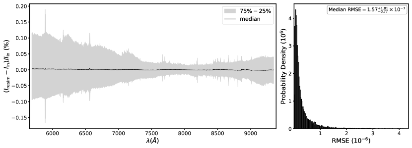
Figure 1: Resimulation results of Settl-Net for the entire synthetic spectra in the test set. The left panel presents the median relative error across the wavelength range of the resimulated spectra based on the MAP predictions of the cINN trained on the Settl models averaged over the 13,107 synthetic spectra in the test set. Here the grey envelope indicates the interquantile range between the $25\%$ and $75\%$ quantiles. In the right panel, we present the histogram of the RMSEs of the 13,107 resimulated spectra. The mean resimulation RMSE across the test set is $3.01\pm 4.35\times 10^{-7}$.

In this section, we validate whether the trained networks well learned the physical rules hidden in the synthetic Phoenix models or not. We use the test set of each database, the synthetic models that are not used for the training but share the same physics as the training data. As mentioned in Sect. 3.2, we only used 80% of the database for training and remained the rest for validation. Each test set consists of 13,107 test models.

5.1.1 Prediction performance

We introduce an accuracy index for evaluating the parameter prediction performance of the network. The accuracy of the prediction is defined as the deviation between the posterior estimate of the parameter and the ground true value ($x^{*}$) of the test model. In this section, we calculate the accuracy in the same physical scales we used to build the databases in Sect. 3.2, meaning that we use the logarithmic scales for the effective temperature and surface gravity and use the linear scale for the extinction magnitude. We use either all posterior estimates sampled for one test model or the maximum a posteriori (MAP) point estimate as a representative. To determine the MAP estimate from the posterior distribution, we perform a Gaussian kernel density estimation on a 1D posterior distribution and find the point where the probability density maximises, similar to the method used in Ksoll et al. (2020) and Kang et al. (2022). In most parts of this paper, we use the MAP estimate to quantify the accuracy of the prediction.

We evaluate the three networks (Settl-Net, NextGen-Net, and Dusty-Net) by using all 13,107 test models in the corresponding test set. For each test model, we sample 4096 posterior estimates and measure the MAP estimates for three parameters from the 1D posterior distributions. In Fig. 13, we present 2D histograms comparing the MAP values estimated by the Settl-Net with the true values of the entire test models. The Settl-Net predicts all three parameters extremely well so the data points are all lying on the 1-to-1 correspondence line. The NextGen-Net and Dusty-Net as well show extremely good results on the test set. The results of the other two networks are very similar to the result of Settl-Net (Fig. 13), so we do not include figures of them in this paper.

To quantify the average accuracy of the network for multiple test models, we measure the root mean square error (RMSE) following,

$$\mathrm{RMSE}=\sqrt{\frac{\Sigma_{i=1}^{N}(x^{\mathrm{MAP}}_{i}-x^{*}_{i})^{2}}{N}}.$$ (6)

In the case of the Dusty-Net, the training ranges of the effective temperature and surface gravity are narrower than that of the other two networks. As the total number of models is the same for all three databases (i.e. 65,536 models), the number density of the model for the effective temperature and surface gravity in the Dusty database is higher than the other two. On this account, we define the normalised RMSE (NRMSE),

$$\mathrm{NRMSE}=\frac{\mathrm{RMSE}}{x_{\mathrm{max}}^{\mathrm{training}}-x_{\mathrm{min}}^{\mathrm{training}}},$$ (7)

by dividing the RMSE by the training range.

In Table 2, we list the RMSE and NRMSE of each parameter for three networks. As already shown in the comparisons between the MAP values and true values (Fig. 13), the RMSE and NRMSE for all three networks are very small around $10^{-4}\sim 10^{-2}$. The Dusty-Net has the smallest RMSE and NRMSE for all three parameters among the three networks. In the case of the effective temperature and extinction, the differences in NRMSE between the networks are very small, whereas the difference in the NRMSE in the case of surface gravity is relatively noticeable among the three parameters. Although the Dusty-Net has the best results, small values in Table 2 demonstrate that all three networks perfectly learned about the synthetic spectra.

5.1.2 Resimulation

To further validate the prediction results of the cINN on the synthetic test data, we verify if the spectra that correspond to the MAP estimates match the respective input spectrum of each test example. We do so by feeding the MAP predictions for the stellar parameters of the 13,107 test examples as an input to our spectra interpolation routine, which we introduced for the training set generation in Sect. 3.1, in order to resimulate the corresponding spectra. Afterwards, we compute the residuals, RMSEs and $R^{2}$ scores of the resimulated spectra in comparison to the corresponding input spectra. The latter serves as a goodness-of-fit measure and is defined as

$$R^{2}=1-\frac{\sum_{i}(y_{i}-\hat{y}_{i})^{2}}{\sum_{i}(y_{i}-\bar{y})^{2}}$$ (8)

for a set of $N$ observations $y_{i}$ with corresponding predictions $\hat{y}_{i}$, where $\bar{y}=\frac{1}{N}\sum_{i}^{N}y_{i}$ denotes the mean of the observations. It takes on values between 0 and 1, with the latter indicating a perfect match (James et al., 2017).

Figure 1 summarises the results for Settl-Net, showing the median relative residual against the wavelength in the left panel and the distribution of RMSEs in the right one. The corresponding plots for NextGen-Net and Dusty-Net can be found in Figs. 14 and 15 in the Appendix. Out of the 13,107 test cases, we could not resimulate spectra for only 52, 32 and 9 MAP predictions for the Settl-Net, NextGen-Net and Dusty-Net, respectively. Only in these few instances either the predicted temperature or gravity (or both) fall outside the interpolation limits of the respective spectra library, such that the spectrum cannot be resimulated. Notably, all of these cases are extreme edge cases, that are right at the training boundaries of either $T_{\mathrm{eff}}$ or $\log(g)$ such that the cINN MAP estimates fall ever so slightly outside the limits while still being an excellent match to the ground truth.

Figure 1 confirms the excellent precision of the MAP predictions demonstrated in the ground truth comparison in Fig. 13. With a median RMSE of the resimulated spectra of $1.57_{-0.77}^{+1.81}\times 10^{-7}$ (and median $R^{2}$ score of $1$), we find that the resimulated spectra are practically spot-on to the corresponding input. In the left panel of Fig. 1 we can also see that, while the overall median residual is very small, there is a systematic trend towards a larger discrepancy between resimulation and input within a shorter wavelength regime ($<7250$ Å). This is likely an effect of the overall low flux in the short wavelength regime for the colder stars ($<4000$ K), such that even a small deviation in flux results in a comparably larger value of the relative residual. Although, it has to be noted again that with most relative deviations falling below $0.2\%$ the discrepancy is overall marginal even in the short wavelength regime.

As Figs. 14 and 15 show, NextGen-Net and Dusty-Net exhibit similar behaviour in the resimulation test, although we find slightly lower mean RMSEs with $2.28\pm 2.48\times 10^{-7}$ and $9.01\pm 7.34\times 10^{-8}$, respectively. Given that the mean RMSEs across the three different spectral libraries agree within one $\sigma$, however, it is safe to say that all three networks achieve equally excellent performance in the resimulation test.

Table 3: Summary of cINN MAP predictions for the Class III template spectra for the cINN models based on the three different spectral libraries.

	MAP estimate
	$T_{\mathrm{eff}}$ (K) [$\Delta_{\mathrm{lit}}$]			$\log(g/\mathrm{cm\,s}^{-2})$ [$\Delta_{\mathrm{lit}}$]			$A_{\mathrm{V}}$ (mag)
Object Name	Settl	NextGen	Dusty	Settl	NextGen	Dusty	Settl	NextGen	Dusty
RXJ0445.8+1556	5391 [379]	5692 [78]	4161 [1609]	4.28 [-0.35]	4.13 [-0.20]	4.14 [-0.21]	0.21	0.38	-0.02
RXJ1508.6-4423	5069 [451]	5434 [86]	4141 [1379]	4.10 [-0.04]	4.16 [-0.10]	4.13 [-0.07]	-0.31	-0.04	-0.13
RXJ1526.0-4501	5150 [260]	5443 [-33]	4170 [1240]	4.25 [0.13]	4.21 [0.17]	4.13 [0.25]	-0.02	0.19	0.14
HBC407	5129 [-19]	5497 [-387]	4165 [945]	4.71 [-0.38]	4.64 [-0.31]	4.26 [0.07]	0.17	0.37	0.02
PZ99J160843.4-260216	5006 [44]	5366 [-316]	4154 [896]	4.43 [-0.95]	4.42 [-0.94]	4.28 [-0.80]	0.15	0.38	-0.09
RXJ1515.8-3331	4895 [155]	5248 [-198]	4177 [873]	4.25 [-0.39]	4.32 [-0.46]	4.31 [-0.45]	0.00	0.32	0.27
PZ99J160550.5-253313	4759 [241]	5168 [-168]	4192 [808]	4.02 [-0.21]	4.19 [-0.38]	4.34 [-0.53]	0.09	0.40	0.21
RXJ0457.5+2014	4644 [356]	5105 [-105]	4123 [877]	4.37 [0.14]	4.63 [-0.12]	4.47 [0.04]	-0.13	0.34	-0.17
RXJ0438.6+1546	4588 [312]	4992 [-92]	4177 [723]	4.01 [0.11]	4.20 [-0.08]	4.50 [-0.38]	0.01	0.44	0.20
RXJ1547.7-4018	4615 [115]	5015 [-285]	4185 [545]	4.15 [0.07]	4.40 [-0.18]	4.52 [-0.30]	-0.02	0.26	0.13
RXJ1538.6-3916	4464 [126]	4830 [-240]	4180 [410]	4.17 [0.04]	4.38 [-0.17]	4.69 [-0.48]	0.01	0.30	0.21
RXJ1540.7-3756	4225 [-20]	4260 [-55]	4115 [90]	4.22 [0.20]	4.17 [0.25]	4.92 [-0.50]	-0.11	0.12	0.22
RXJ1543.1-3920	4269 [-64]	4299 [-94]	4132 [73]	4.34 [-0.22]	4.32 [-0.20]	5.00 [-0.88]	0.03	0.28	0.39
SO879	4106 [-46]	4027 [33]	3909 [151]	3.96 [-0.06]	4.09 [-0.19]	4.78 [-0.88]	0.22	0.29	-0.12
Tyc7760283_1	3881 [-31]	3748 [102]	3742 [108]	5.00 [-0.30]	4.99 [-0.29]	5.23 [-0.53]	-0.17	-0.34	-0.52
TWA14	3819 [-39]	3739 [41]	3677 [103]	5.07 [-0.37]	4.87 [-0.17]	5.09 [-0.39]	-0.32	0.19	-0.30
RXJ1121.3-3447_app2	3797 [-92]	3622 [83]	3635 [70]	4.78 [-0.18]	4.68 [-0.08]	5.13 [-0.53]	0.38	0.30	0.02
RXJ1121.3-3447_app1	3719 [-14]	3559 [146]	3564 [141]	4.90 [-0.10]	4.77 [0.03]	5.16 [-0.36]	0.01	0.04	-0.07
CD_29_8887A	3670 [-110]	3483 [77]	3491 [69]	4.79 [-0.39]	4.57 [-0.17]	5.05 [-0.65]	0.56	0.51	0.07
CD_36_7429B	3423 [-8]	3264 [151]	3262 [153]	4.70 [-0.20]	4.44 [0.06]	4.82 [-0.32]	0.52	0.50	0.13
TWA15_app2	3467 [-52]	3289 [126]	3306 [109]	4.93 [-0.53]	4.71 [-0.31]	5.02 [-0.62]	0.17	0.31	0.09
TWA7	3519 [-104]	3321 [94]	3316 [99]	4.83 [-0.23]	4.45 [0.15]	4.80 [-0.20]	0.41	0.94	0.14
TWA15_app1	3469 [-129]	3285 [55]	3310 [30]	5.01 [-0.51]	4.79 [-0.29]	5.08 [-0.58]	0.06	0.20	0.10
SO797	3248 [-48]	3225 [-25]	3078 [122]	3.93 [-0.03]	3.47 [0.43]	4.03 [-0.13]	1.07	1.48	0.73
SO641	3129 [-4]	3237 [-112]	2997 [128]	3.86 [-0.06]	3.20 [0.60]	3.81 [-0.01]	0.68	1.46	0.43
Par_Lup3_2	3181 [-56]	3245 [-120]	3048 [77]	3.96 [-0.26]	3.29 [0.41]	4.00 [-0.30]	0.72	1.29	0.40
SO925	3008 [52]	3277 [-217]	2961 [99]	3.76 [-0.06]	2.92 [0.78]	3.61 [0.09]	0.97	2.01	0.76
SO999	3079 [-19]	3294 [-234]	2979 [81]	3.68 [0.12]	2.85 [0.95]	3.58 [0.22]	0.69	1.60	0.54
Sz107	2981 [79]	3272 [-212]	2935 [125]	3.69 [0.11]	2.85 [0.95]	3.50 [0.30]	0.56	1.67	0.35
Par_Lup3_1	2739 [196]	3170 [-235]	2868 [67]	3.53 [-0.03]	2.37 [1.13]	3.04 [0.46]	2.74	3.62	2.47
LM717	2714 [221]	3218 [-283]	2903 [32]	3.46 [0.14]	2.37 [1.23]	2.84 [0.76]	1.83	3.08	1.82
J11195652-7504529	2629 [251]	3165 [-285]	2864 [16]	3.50 [-0.41]	2.27 [0.82]	2.75 [0.34]	2.11	3.43	2.24
LM601	2601 [194]	3137 [-342]	2807 [-12]	3.62 [-]	2.28 [-]	2.98 [-]	1.79	3.16	2.00
CHSM17173	2539 [171]	3096 [-386]	2773 [-63]	3.50 [-]	2.18 [-]	2.61 [-]	1.66	3.45	2.31
TWA26	2477 [-77]	2959 [-559]	2625 [-225]	3.46 [0.14]	1.83 [1.77]	2.56 [1.04]	2.64	3.92	2.92
DENIS1245	2453 [-123]	2924 [-594]	2590 [-260]	3.45 [0.15]	1.71 [1.89]	2.58 [1.02]	2.34	3.74	2.82

5.2 Validations with Class III template stars

In this section, we investigate how well our cINNs predict each parameter when applied to real observations by analysing Class III template stars introduced in Sect. 4. Stellar parameter values (i.e. effective temperature, surface gravity, and extinction) provided by previous papers (Manara et al., 2013, 2017; Stelzer et al., 2013) are listed in Table 1. Among the 36 template stars, there are cases where the literature value of effective temperature is out of the training range of the cINNs, or where the literature value of gravity is missing. Two out of 36 stars have temperatures below 2600 K, outside the temperature range of all three databases. Also, 14 stars with temperatures between 4000 K and 7000 K are out of the training range of the Dusty-Net. These stars will be excluded from some analyses in the following sections.

Using each network, we sample 4096 posterior estimates per star and measure MAP estimation for three parameters. We list the MAP values predicted by three networks in Table 4.

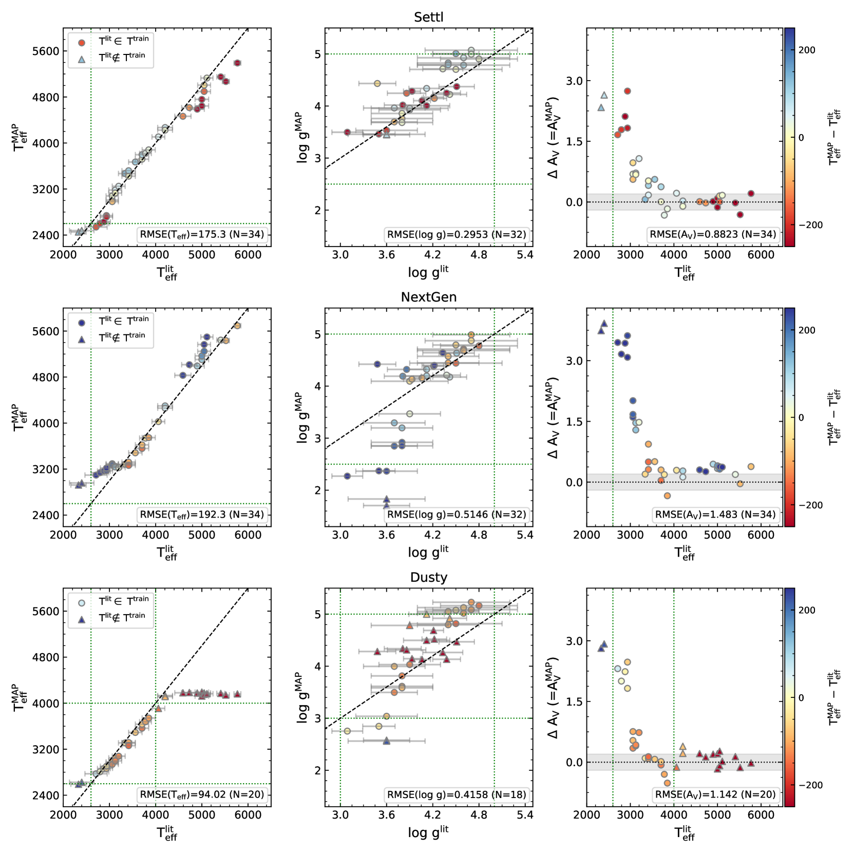
Figure 2: Comparison of MAP predictions with literature values in Table 1. Stars are basically denoted by circle symbols but triangle symbols denote stars excluded in analyses such as RMSE calculation either because their literature values of temperature are out of the cINN training range or because their literature values of surface gravity are missing. The colour indicates the temperature deviation between the MAP estimate and the literature value. We indicate the training range of each parameter with green dotted lines. In the third column, the grey horizontal area presents the 1-$\sigma$ uncertainty (i.e. 0.2 mag) of extinction provided by literature.

5.2.1 Parameter comparison between literature and cINN

In Fig. 2, we compare the stellar parameter values from literature ($x_{\mathrm{lit}}$) with MAP predictions ($x_{\mathrm{MAP}}$). Each row shows the result of different cINNs. The first two columns are the results of effective temperature and surface gravity. As the extinction value of template stars is negligible, we compare the literature value of the temperature with the MAP estimation of extinction. We calculate the uncertainty of the MAP estimate based on the width of the posterior distribution, but as the uncertainties are all very small, we did not present the uncertainty of the MAP estimate in the figure. For the uncertainty of the literature values, we adopt a 1-subclass temperature interval as the uncertainty of temperature and use the surface gravity uncertainty provided by the literature (Stelzer et al., 2013; Manara et al., 2017). According to the literature, the 1-$\sigma$ uncertainty of extinction is $\sim$ 0.1–0.2 mag, so we indicate from $-0.2$ to $0.2$ mag range in grey to show the uncertainty range.

In this section, we do not use some stars in our analyses where the stellar parameter value from literature is out of the training range or where any stellar parameter value is missing, although they are presented in Fig. 2 by triangle symbol. We use 34, 34, and 20 stars for Settl-Net, NextGen-Net, and Dusty-Net, respectively when analysing temperatures or extinction, and use 32, 32, and 18 stars respectively when analysing gravity.

Comparing the temperature MAP estimates with the literature values, we confirm that the majority of stars are lying close to the 1-to-1 correspondence line. We calculate the RMSE for each network by only using stars whose temperature literature values are within the training range (i.e. circle markers in Fig. 2). Considering that the average of the 1-subclass temperature interval of these stars is about 140 K, the RMSE values of 175.3 K, 192.3 K, and 94.02 K for Settl-Net, NextGen-Net, and Dusty-Net, respectively, are well within 1 to 2 subclasses interval. As shown in the figure and RMSE values, Dusty-Net has the best agreement with the literature value when the temperature is within its training range of 2600 – 4000 K. However, Dusty-Net shows very poor agreement with the literature values when the temperature is outside the training range. This implies the caution of using cINN to analyse stars far from the training range. Comparing Settl-Net and NextGen-Net having the same training range, MAP estimates of Settl-Net are closer to the literature values.

To compare the performance of the three networks on the temperature in more detail, we present the relative temperature deviations between the MAP predictions and the literature values sorted by their spectral type. Figure 3 as well shows that MAP estimates from Dusty-Net are in good agreement with the literature value within a 5 per cent discrepancy. In the case of Dusty-Net, all but one star have a deviation within the 1-subclass interval. In the case of Settl-Net and NextGen-Net, 23 and 16 stars out of 34, respectively, have a deviation less than a 1-subclass interval. MAP estimates of Settl-Net and NextGen-Net have a relatively poor agreement with the literature values for hot stars of $4500\,$K (e.g. K4.0 type) or higher. However, the discrepancies are still within 10 per cent. The average absolute relative deviations when only using the templates within the training range of each network are 3.28, 4.49, and 2.58 per cent for Settl-Net, NextGen-Net, and Dusty-Net, respectively (Table 4). These average errors are equivalent to 1.08, 1.12, and 0.601 subclasses.

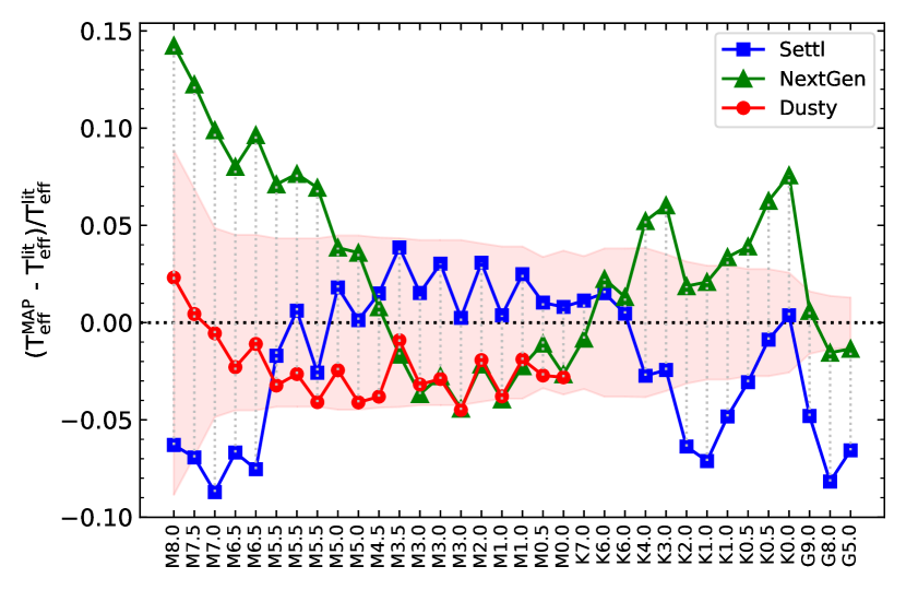
Figure 3: Relative temperature deviations of the template stars between the MAP estimates and the literature values sorted by their spectral type. Different colours and symbols indicate the results of three different cINNs. The pink area indicates the uncertainty of the literature value of temperature. We only present template stars whose literature value of temperature is within the network training range.

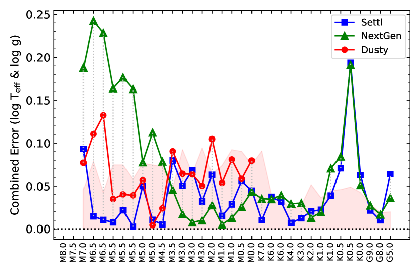
Figure 4: Average relative error of the template stars between the MAP estimates and the literature values sorted by their spectral type. The average error is calculated as a root mean square of the relative errors of temperature and gravity, both in log-scale (Eq. 9). The pink area indicates the 1-$\sigma$ uncertainty of the literature value. We only present template stars whose literature value of temperature is within the network training range and whose literature value of gravity is presented. Colour codes are the same as in Fig. 3.

Table 4: Average absolute relative error between cINN predictions and literature values for template stars.

	Average relative error [%]			Average relative error [$\sigma$]
Network	$T_{\mathrm{eff}}$	$\log(g)$	$A_{\mathrm{V}}$	$T_{\mathrm{eff}}$	$\log(g)$	$A_{\mathrm{V}}$
Settl	3.28	5.5	-	1.08	0.809	2.78
NextGen	4.49	10.2	-	1.12	1.38	4.95
Dusty	2.58	9.13	-	0.601	1	3.87

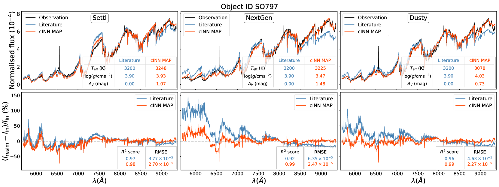
Figure 5: Resimulation results for Class III star SO797. The columns show in order the results for the three different spectral libraries Settl, NextGen and Dusty. Top: Comparison of resimulated spectrum. The blue spectrum indicates the resimulation derived from the literature stellar parameters from Table 1. The red spectrum shows the corresponding resimulation based on the cINN MAP prediction. The respective input parameters for the resimulation are summarised in the table in the bottom right corner. The relative residuals $(I_{\mathrm{resim}}-I_{\mathrm{in}})/I_{\mathrm{in}}$ of the resimulated spectra compared to the input spectrum are shown in the bottom panels, respectively.

In the case of surface gravity, the RMSE of Settl-Net, NextGen-Net, and Dusty-Net are 0.30, 0.51, and 0.42 dex, respectively. However, because the surface gravity value from previous studies (Stelzer et al., 2013; Manara et al., 2017) is obtained by fitting the spectrum on the Settl models, the MAP estimate of Settl-Net is essentially the closest to the literature value. Although Settl-Net has the smallest RMSE value, considering the uncertainty of literature values, the other two networks also have good agreement with the literature value.

To combine the results of temperature and surface gravity, we define the combined error of two parameters as,

$$\begin{split}\mathrm{Combined\>error}&=\sqrt{\frac{1}{2}\left(\left(\frac{\Delta T_{\mathrm{eff}}}{\mathrm{log}\,T^{\mathrm{lit}}_{\mathrm{eff}}}\right)^{2}+\left(\frac{\Delta g}{\mathrm{log}\,g^{\mathrm{lit}}}\right)^{2}\right)},\\ \>\mathrm{for}\\ \Delta T_{\mathrm{eff}}&=\mathrm{log}\,T^{\mathrm{MAP}}_{\mathrm{eff}}-\mathrm{log}\,T^{\mathrm{lit}}_{\mathrm{eff}},\\ \Delta g&=\mathrm{log}\,g^{\mathrm{MAP}}-\mathrm{log}\,g^{\mathrm{lit}},\end{split}$$ (9)

and present the combined error of each template star. We use the effective temperature in the logarithmic scale to match the scale with surface gravity. The overall result using combined error presented in Fig. 4 are not significantly different from Fig. 3, but by adding the gravity error, Settl-Net shows better performance than Dusty-Net even for low-temperature stars. In the case of NextGen-Net, the combined error is larger than the other two networks because there are cases where temperature and gravity errors are both large. The average combined errors across the stars of Settl-Net  NextGen-Net, and Dusty-Net are 3.93, 7.20, and 6.47 per cent, respectively.

In the case of Settl-Net, all but 7 stars are in good agreement with the literature values within 1-$\sigma$ uncertainty. Excluding one star with a large error, most of the stars have errors of less than 5 per cent and a maximum of 10 per cent. Dusty-Net also has small errors ($<$15 per cent) but Dusty-Net has a disadvantage in that it is inherently less versatile than the other two networks because of its training range. NextGen-Net also shows an error of less than 10 per cent for stars with spectral type earlier than M5.0.

Lastly, in the case of extinction, the deviation between MAP estimates and literature values varies depending on the temperature. For stars hotter than about 3400 K (i.e. M3.0 type), all three networks predict near-zero extinction, with little deviation from literature values. In the case of NextGen-Net, there are stars that are slightly outside the error range but their MAP estimates are sufficiently small. On the other hand, for cool stars below 3400 K, the discrepancy between the MAP value and the literature value gradually grows. In the case of Settl-Net and Dusty-Net, the MAP estimate does not exceed the maximum of 3, but in the case of NextGen-Net, the MAP estimates are slightly larger than the other two networks.

In this section, we showed that the discrepancy between the network MAP prediction and literature value varies with the characteristics of the stars. Based on the overall results, a star of

• M6.5 – K1.0 (2935 – 5000 K) for Settl-Net,

• M4.5 – K1.0 (3200 – 5000 K) for NextGen-Net,

• M5.5 – M0.0 (3060 – 4000 K) for Dusty-Net

shows especially high agreement with the literature values. Settl-Net showed the best agreement with the literature values overall. Dusty-Net also shows a good agreement for stars whose temperature is within the Dusty database of 2600 – 4000 K. NextGen-Net has relatively large errors compared to the other two, but it still shows reliable performance for early-type stars. Given that Settl-Net and NextGen-Net cover a wider range of temperature (i.e. 2600 – 7000 K) and gravity (2.5 – 5 $\log(\mathrm{cm\,s}^{-2})$) than Dusty-Net, Settl-Net is the best choice among the three networks. However, all three networks showed good agreement with the literature values considering their uncertainty.

This result shows how well our cINN predictions are in good agreement with values obtained with the classical methods in previous studies. Differences between literature values and network predictions do not demonstrate that the network prediction is wrong. For example, in the case of surface gravity, because the literature value was also obtained by fitting spectra based on the Settl model, there is inevitably a larger discrepancy between the literature values and MAP predictions of NextGen-Net and Dusty-Net. This means that we need to consider methods used in the literature, and additional analysis is required to judge whether the cINN prediction is really wrong or not. The resimulation following in the next section will provide a better clue to determine the correctness of our cINN predictions.

5.2.2 Resimulation

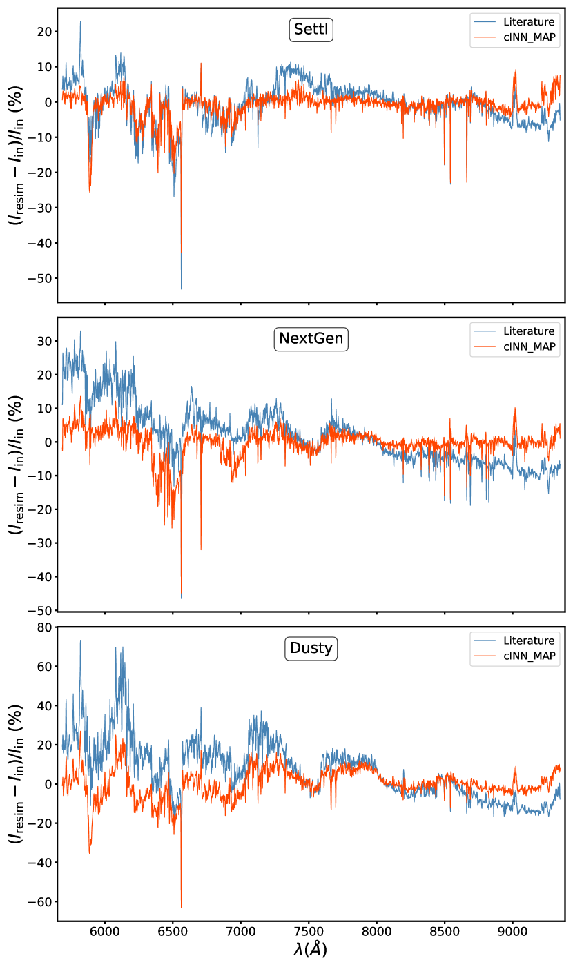
Figure 6: Comparison of the median relative error of the resimulated spectra for the Class III template stars between the resimulations based on the literature stellar parameters (blue, see Table 1) and the cINN MAP predictions (red). From top to bottom, the panels show the corresponding results for the three tested spectral libraries Settl, NextGen and Dusty.

As we have done for the synthetic test data in Sect. 5.1.2, we also evaluate the accuracy of the cINN predictions on the Class III template by resimulation to quantify the agreement between the spectra corresponding to the MAP estimates with the input spectra. In this case, we also run a resimulation for the nominal literature stellar parameters of the Class III sources listed in Table 1 for comparison. Some of the Class III template sources in our sample do not have an estimate for $\log(g)$ in the literature. For these sources, we assume a fixed value of $\log(g/\mathrm{cms}^{-2})=4.0$ in our resimulation, which is a reasonable guess for the spectral types in our sample. The sources in question are marked as ”fixed” in the last column of Table 1. There are a few templates (7 for Settl, 1 for NextGen and 8 for Dusty; see Table 4), where the cINN extinction MAP estimate has a non-physical negative value. Since most of these are only barely below zero, we decide to allow these negative values to be accounted for during the resimulation.

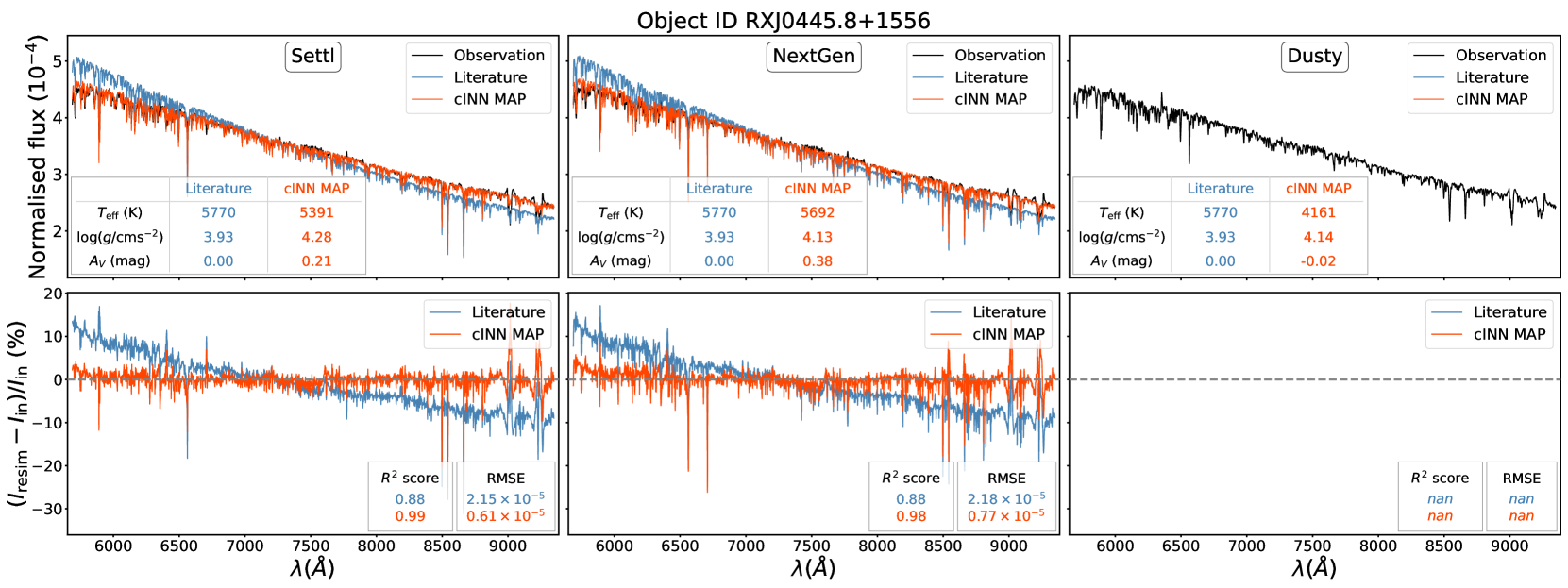
Figure 16: Resimulation results for Class III star RXJ0445.8+1556. Same as Fig. 5.

Figure 5 shows an example result of the resimulation for the M4-type template star SO797 for all three spectral libraries with the top panels comparing the resimulated spectra to the input spectrum and bottom panels showing the corresponding residuals. Here the red curve indicates the resimulation result derived from the cINN MAP estimates, whereas the blue curve marks the literature-based outcome. In this particular example, the cINN recovers both $T_{\mathrm{eff}}$ and $\log(g)$ quite accurately for all three spectral libraries but overestimates $A_{V}$ for this supposedly zero extinction template Class III source by $1.07$, $1.48$ and $0.73$ mag based on Settl, NextGen and Dusty, respectively. Interestingly, however, we find that the resimulated spectrum based on the cINN MAP prediction with the supposedly wrong $A_{\mathrm{V}}$ matches the input spectrum better than the spectrum derived from the literature value in all three examples as e.g. attested by the smaller RMSE and better $R^{2}$ score of $2.7\times 10^{-5}$ and $0.98$ compared to $3.77\times 10^{-5}$ and $0.97$ in the Settl case. Figure 16 in the Appendix shows another such example, where it is immediately apparent that the cINN-based resimulated spectrum matches the input observation much better than the literature-based solution, which evidently does not capture the slope of the observed spectrum correctly.

Figures 6, 7 and Table 6 in the Appendix summarise the resimulation results across the entire Class III template sample, showing the median relative residuals against the wavelength, the distributions of RMSEs and $R^{2}$ scores, and a table of all RMSEs and $R^{2}$ scores, respectively. Note that the resimulation statistics vary between the libraries here. Given the lower effective temperature limits of the libraries (i.e. $2600$ K) 2 of the 36 templates, namely TWA26 and DENIS1245, can a priori not be resimulated with Settl and NextGen. For Dusty, the literature sample is even smaller with only 20 out of 36 templates due to the low upper temperature limit of 4000 K. For the resimulation of the MAP estimates we can use 31 templates with the Settl-Net, 29 with NextGen-Net and only 17 with Dusty-Net. For more details, we refer to Table 6. Note that for the Dusty resimulation there are actually 7 templates, where the $\log(g)$ prediction is above the training set limit of 5. However, since the Dusty spectral library does actually extend to $\log(g/\mathrm{cms}^{-2})=5.5$, we decide to run the resimulation for these 7 templates anyways, in particular since for most of those the $\log(g)$ prediction is only barely above 5 (see Table 4).

Figure 6 shows that for all three libraries, we find that our observation from Fig. 5, where the resimulated spectrum based on the cINN prediction fits the input spectrum better than the literature-based resimulation, holds on average across the entire template sample. The distributions of the RMSEs and $R^{2}$ scores of the resimulated spectra in Fig. 7 further confirm this, as the cINN-based resimulated spectra tend towards smaller RMSEs and slightly better $R^{2}$ scores compared to the literature-based spectra for all three spectral libraries.

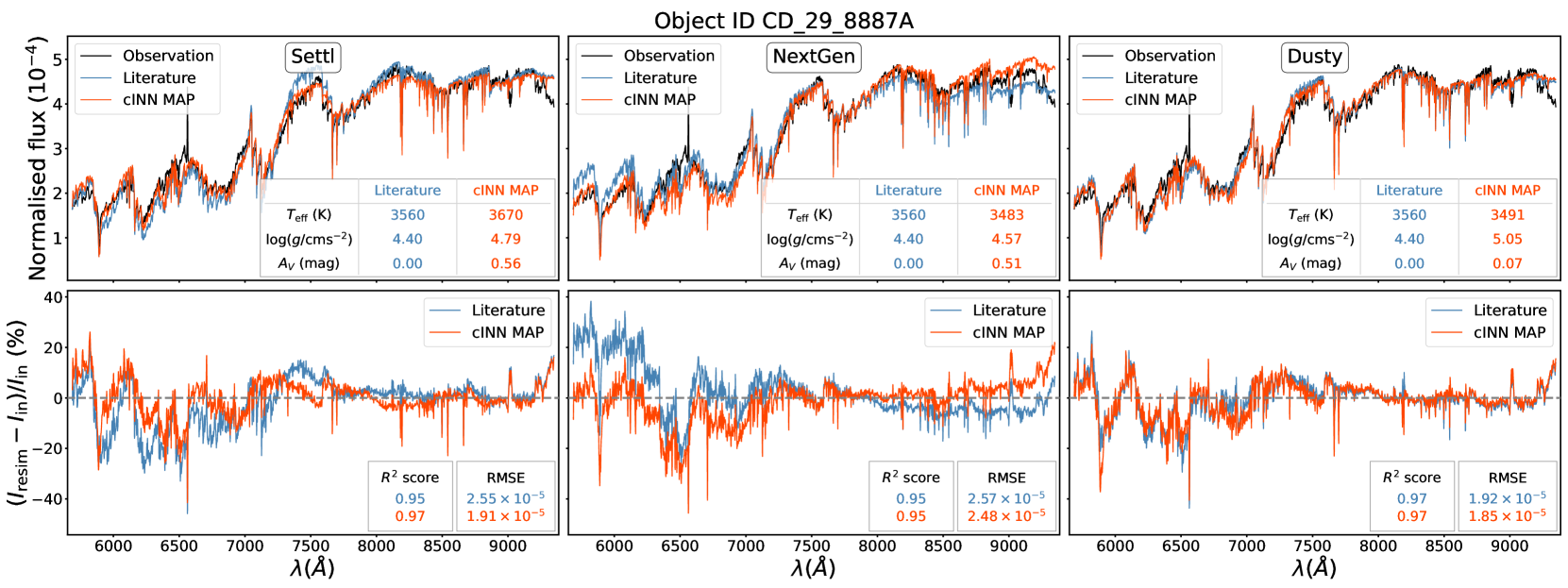
Figure 17: Resimulation results for Class III star CD_29_8887A. Same as Fig. 5.

Examining the 7 templates, for which the Dusty-based cINN prediction of $\log(g)$ exceeds the learned upper limit of 5 (i.e. the cINN extrapolated), more closely, the resimulation results show that even when the cINN extrapolates, the set of predicted parameters corresponds to a spectrum, which matches the input observation quite well and, in particular, equally if not better than the respective spectrum resimulated from the literature values as indicated by the $R^{2}$ scores (see Table 6 and Fig. 17 for an example). This result shows that the cINN prediction is actually fairly robust even in the event of slight extrapolation.

Comparing our chosen resimulation accuracy measures to the spectral types of the Class III templates in Fig. 8, we find that the RMSEs exhibit an increasing trend towards the M-types for all three spectral libraries. For the $R^{2}$ scores, we find a notable dip in the goodness of fit for the intermediate spectral types, that is between M2 to K3, in both the resimulation of the literature and cINN-based values for Settl and NextGen. The beginning of this dip can also be seen in the Dusty-based results up to the temperature limit of this library at the K7 type. Interestingly, when compared to Fig. 4 in this spectral type range the discrepancy between the cINN prediction and literature stellar properties is relatively low, where both cINN and literature values correspond to an equally sub-optimal fit to the observed spectra.

Overall the resimulation test shows that the cINN approach predicts parameters for the real Class III template spectra that correspond to spectra, which not only fit the input observations very well (as shown by the good $R^{2}$ scores in Fig. 7 and Table 6), but also match better than the spectra resimulated from the literature values in most instances.

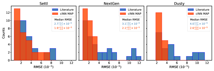
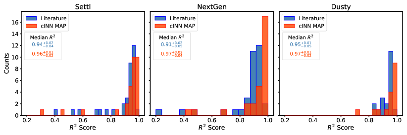
Figure 7: Average error for the resimulation spectra for the Class III template stars. Top: Histograms of the RMSEs for the resimulation on the Class III template spectra for the three different spectral libraries. Bottom: Histograms of the corresponding $R^{2}$ scores for the resimulated spectra.

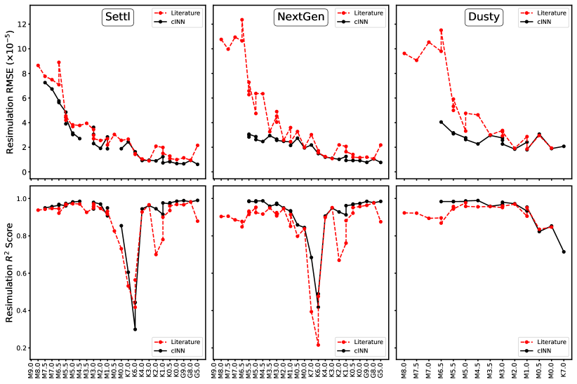
Figure 8: Comparison of the resimulation accuracy measures (RMSE in the top row, $R^{2}$ score in the bottom) for the three spectra libraries to the spectral type of the Class III templates. In all panels, the dotted red line indicates the results for the resimulation based on the literature stellar properties, while the black line shows the cINN-based outcomes.

6 Feature importance

6.1 Importance calculation

In this section, we evaluate which parts of the spectra the cINN prediction relies the most upon. To do so we measure the so-called permutation feature importance, an approach first described by Breiman (2001) for random forest models and later generalised by Fisher et al. (2018). In this study we implement the Fisher et al. (2018) algorithm as described in Molnar (2022), operating as follows:

First, we compute the error on the original held-out test set

$$e_{\mathrm{orig}}=L\left(\mathbf{X},g(\mathbf{Y})\right),$$ (10)

where $g$ represents the inverse translation ($\mathbf{x}\leftarrow\mathbf{y}$) of the trained cINN, $\mathbf{X}$ denotes the matrix of the target parameters of the test set ($n_{\mathrm{test}}\times n_{\mathrm{parameters}}$), $\mathbf{Y}$ is the $n_{\mathrm{test}}\times n_{\mathrm{features}}$ feature matrix of the test set and $L$ represents a loss measure. In our case, $L$ is the RMSE of the MAP estimates.

Next, for each feature $j\in\{1,\ldots,n_{\mathrm{features}}\}$, we generate a feature matrix $\mathbf{Y}_{\mathrm{perm},j}$ via random permutation of the $j$-th column in order to break the association between feature $j$ and the target parameters $\mathbf{x}$, estimate the prediction error $e_{\mathrm{perm},j}=L\left(\mathbf{X},g\left(\mathbf{Y}_{\mathrm{perm},j}\right)\right)$ based on the permuted data set, and compute the feature importance of feature $j$ as the quotient

$$\mathrm{FI}_{j}=\frac{e_{\mathrm{perm},j}}{e_{\mathrm{orig}}}.$$ (11)

The larger $\mathrm{FI}_{j}$ is, the worse the model prediction becomes if feature $j$ is scrambled via permutation, that is the more important feature $j$ is to the model’s decision making. The closer $\mathrm{FI}_{j}$ is to 1, on the other hand, the less feature $j$ affects the predictive performance and, thus, the less relevant it is to the model’s reasoning.

In our particular case, the feature space is very high dimensional with $2930$ spectral bins per spectrum. Consequently, computing the individual per spectral bin feature importance is rather computationally expensive as it requires generating the posteriors and determining the MAP estimates for each of the $2930$ bins. Although the computational cost alone is not prohibitive in this case given the cINNs great efficiency, we still opt for a slightly different approach, because the spectral bins themselves are also not necessarily independent of each other. Instead of using the individual bins, we group them together into combined features, for which we then estimate the importance. In practise, this means that we permute multiple columns at once (each column with its own permutation seed though) corresponding to the spectral bins in a given group. For the setup in this study in particular we decide to evaluate the feature importance across the wavelength range using groups of 10 bins, which corresponds to a spectral width of $12.5$ Å. We set all groups to overlap by 5 bins (i.e. $6.25$ Å) with the preceding and following groups. We average feature importance for overlapping bins.

6.2 Important features for M-, K-, and G-type stars

Figure 9: Feature importance evaluation for M-type synthetic models in the test set using Settl-Net. We present the median flux of M-type Class III template stars in the first row. The grey area indicates the interquantile range between the 25% and 75% quantiles. The other three rows show the feature importance across the wavelength for each stellar parameter. Vertical lines and shades indicate the location of typical tracers of stellar parameters listed in Table 5.

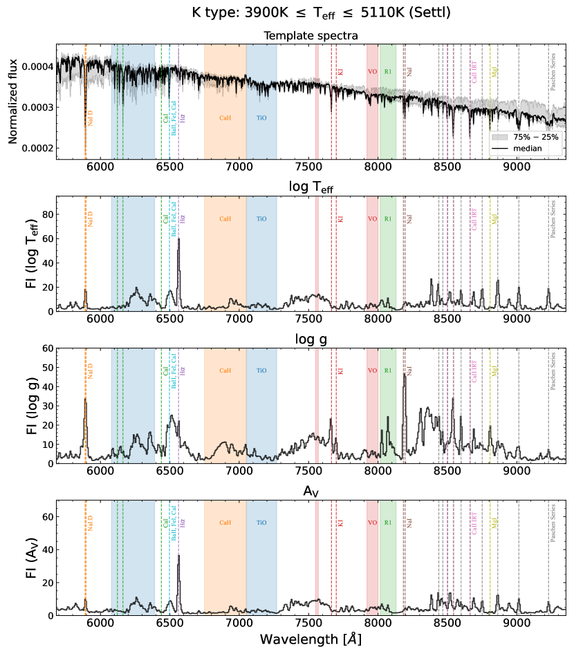
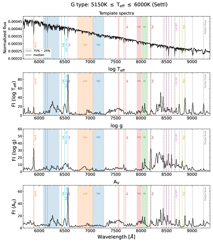
Figure 10: Feature importance evaluation for K-type synthetic models (left) and for G-type synthetic models (right) in the test set using Settl-Net. The panels in the first row show the median flux of K-type and G-type Class III template stars, respectively. Lines and shades are the same as Fig. 9.

We draw three groups from the test set according to the temperature of the test model: M-type (2600K–3850 K) group, K-type (3900K–5110 K) group, and G-type (5150K–6000 K) group, and evaluate the feature importance across the wavelength for each group per network. In the case of Dusty-Net, we only evaluate for the M-type group because the maximum temperature of the Dusty database is 4000 K.

Figure 9 presents the feature importance of Settl-Net for M-type stars. To compare the important features with the locations of stellar parameter tracers existing in the real spectrum, we plot the median flux of M-type template stars in the first row, and indicate the locations of several tracers of stellar parameters (Table 5): Na i doublet $5890$, $5896$ Å ($T_{\mathrm{eff}}$ and $\log{g}$, Allen & Strom, 1995), Ca i $6122$, $6162$, $6439$ Å ($\log{g}$, Allen & Strom, 1995), Ba ii, Fe i, and Ca i blend 6497 Å ($T_{\mathrm{eff}}$ and $\log{g}$, Allen & Strom, 1995; Herczeg & Hillenbrand, 2014), H$\mathrm{\alpha}$ $6563$ Å ($T_{\mathrm{eff}}$, Luhman et al., 2003), K i doublet $7665$, $7699$ Å ($T_{\mathrm{eff}}$ and $\log{g}$, Manara et al., 2013, 2017), Na i doublet $8183$, $8195$ Å ($T_{\mathrm{eff}}$ and $\log{g}$, Kirkpatrick et al., 1991; Allen & Strom, 1995; Riddick et al., 2007), Ca ii IR triplet $8498$, $8542$, $8662$ Å ($T_{\mathrm{eff}}$, Kirkpatrick et al., 1991; Allen & Strom, 1995; Luhman et al., 2003), Mg i $8807$ Å ($T_{\mathrm{eff}}$, Manara et al., 2013; Herczeg & Hillenbrand, 2014), hydrogen Paschen series ($A_{\mathrm{V}}$, Edwards et al., 2013), CaH $6750$–$7050$ Å ($T_{\mathrm{eff}}$ and $\log{g}$, Kirkpatrick et al., 1993; Allen & Strom, 1995), TiO $6080$–$6390$, $7053$–$7270$ Å ($T_{\mathrm{eff}}$, Kirkpatrick et al., 1991; Henry et al., 1994; Jeffries et al., 2007), ViO $7550$–$7570$, $7920$–$8000$ Å ($T_{\mathrm{eff}}$, Allen & Strom, 1995; Riddick et al., 2007; Manara et al., 2013), and R1 $8015$–$8130$ Å ($T_{\mathrm{eff}}$, Riddick et al., 2007) .

To evaluate whether these observational tracers act as important features in our networks, we check whether the feature importance value corresponding to each tracer’s wavelength is larger than a fiducial value. We use the value of median plus one standard deviation over the entire wavelength range as a fiducial value to determine an important tracer. For tracers with multiple lines or molecular bands, we average the feature importance for each line or over the wavelength range. In Table 5, we mark tracers whose average importance is larger than the fiducial value. We also indicate for which parameters these lines and bands trace in real observations.

Figure 9 shows that Na i doublet $8183$, $8195$ Å lines are the most important feature for Settl-Net to predict stellar parameters of M-type stars. In the case of extinction, there are two wide peaks near 7500 Å, where the redder peak overlaps with the VO molecular band. However, Na i has a similarly large importance value. In the case of temperature and gravity, K i doublet $7665$, $7699$ Å lines play a second important role, and in extinction, H$\mathrm{\alpha}$ does. VO and R1 molecular absorption bands as well act as important features to determine the temperature and extinction.

We present the feature importance evaluated for NextGen-Net and Dusty-Net in Fig. 19. The fact that Na i, K i, and H$\mathrm{\alpha}$ are important features for M-type stars is the same for all three networks. However, for NextGen-Net, there is a large bump at 7500 Å in the case of temperature. The results of NextGen-Net in overall are spikier than in the other two networks. In the case of Dusty-Net, the importance value of Na i doublet $5890$, $5896$ Å (Na i D) is relatively large compared to the other networks, and there is a very wide bump around Na i doublet $8183$, $8195$Å.

Given the fact that extinction affects the overall shape of the spectrum, it is interesting that the Settl-Net relies a lot on a few certain lines. Broad bumps exist in the red part of the spectrum, but there are particularly important lines and areas such as the Na i, H$\mathrm{\alpha}$, and near VO bands. The result of NextGen-Net is similar to Settl-Net but shows a little more spiky trend with wider peaks. Dusty-Net shows a more wavy shape across the entire wavelength range compared to the others.

Next, in the case of K-type stars, the results of Settl-Net and NextGen-Net are similar to each other, unlike the case of M-type stars, so we only present the result of Settl-Net in this paper (left panels in Fig. 10). Compared to the results of M-type stars, it is noticeable that important features are different for each parameter. In the case of temperature and extinction, the overall shapes are similar, with the H$\mathrm{\alpha}$ line being the most important feature. Na i doublet $8183$, $8195$ Å are no longer so important to determine temperature and extinction for K-type stars. In addition, Na i D lines and hydrogen Paschen series have relatively high importance values. On the other hand, in the case of surface gravity, the Na i doublet $8183$, $8195$ Å lines still play the most important role. The importance of Na i D in gravity becomes noticeable in K-type stars compared to M-type stars. Additionally, there are several peaks at K i, Mg i $8807$ Å used as important features to determine gravity.

The result of G-type stars (i.e. right panels in Fig. 10) is similar to the K-type stars. The H$\mathrm{\alpha}$ is still the most important feature for temperature and extinction and there are several peaks at the Paschen series as well. For gravity, Na i D becomes more important in G-type stars and has an importance value comparable to that of Na i doublet $8183$, $8195$Å. These sodium lines are the most important features to determine gravity. On the other hand, the importance of K i lines decreases in G-type stars compared to K-type stars.

Table 5: We mark tracers whose feature importance values are larger than the fiducial value of median plus 1 standard deviation, meaning that marked tracers are significantly important features to determine each stellar parameter.

		M-type			K-type			G-type
Tracers	used in observations for	$T_{\mathrm{eff}}$	$\log(g)$	$A_{\mathrm{V}}$	$T_{\mathrm{eff}}$	$\log(g)$	$A_{\mathrm{V}}$	$T_{\mathrm{eff}}$	$\log(g)$	$A_{\mathrm{V}}$
Na i doublet $5890$, $5896$ Å	$T_{\mathrm{eff}}$, $\log(g)$	-	-	-	✓	✓	✓	✓	✓	✓
TiO $6080$–$6390$, $7053$–$7270$ Å	$T_{\mathrm{eff}}$ (M- and late K-type)	-	-	-	-	-	-	-	-	-
Ca i $6122$, $6162$, $6439$ Å	$\log(g)$	-	-	-	-	-	-	-	-	-
Ba ii, Fe i, and Ca i blend 6497 Å	$T_{\mathrm{eff}}$, $\log(g)$	-	-	-	✓	-	✓	✓	-	✓
H$\mathrm{\alpha}$ $6563$ Å	$T_{\mathrm{eff}}$ (early type)	-	-	✓	✓	✓	✓	✓	✓	✓
CaH $6750$–$7050$ Å	$T_{\mathrm{eff}}$ (M-type), $\log(g)$	-	-	-	-	-	-	-	-	-
VO $7550$–$7570$, $7920$–$8000$ Å	$T_{\mathrm{eff}}$ (M-type)	✓	✓	✓	✓	✓	✓	✓	-	✓
K i doublet $7665$, $7699$ Å	$T_{\mathrm{eff}}$, $\log(g)$	✓	✓	✓	-	-	-	-	-	-
R1 $8015$–$8130$ Å	$T_{\mathrm{eff}}$ (M-type)	✓	✓	✓	-	-	-	✓	✓	-
Na i doublet $8183$, $8195$ Å	$T_{\mathrm{eff}}$ (M-type), $\log(g)$	✓	✓	✓	✓	✓	-	-	✓	✓
hydrogen Paschen series	$A_{\mathrm{V}}$	-	-	-	✓	✓	✓	✓	✓	✓
Ca ii IR triplet $8498$, $8542$, $8662$ Å	$T_{\mathrm{eff}}$ (early type)	✓	✓	-	✓	✓	-	✓	✓	✓
Mg i $8807$ Å	$T_{\mathrm{eff}}$	-	-	-	-	✓	-	-	✓	-

These results show that the features that our networks rely on to determine parameters vary depending on the input object. In particular, when changing from M- to K-type, important features change noticeably. For example, the Na i doublet $8183$, $8195$ Å lines are essential features for networks to understand M-type stars, sensitive to all three stellar parameters, but for earlier type stars (K- and G-types), it is important only to determine gravity. Similarly, the K i doublet lines are gravity-sensitive features for late-type stars but they are less essential for earlier types. In the case of Na i doublet $5890$, $5896$ Å lines, on the other hand, they are more important for hot stars rather than for cold stars to determine gravity.

Please note that the feature-importance tests presented in this section indicate the features that affect the network’s judgement which is based on the Phoenix models. Some of the important features (that are essential for the network) behave very similarly to our knowledge, but some do not. Above all, the behaviour of the Na i doublet $8183$, $8195$ Å lines in the feature importance test agrees well with our knowledge. The Na i line, tracing the gravity (Riddick et al., 2007; Herczeg & Hillenbrand, 2014; Manara et al., 2017) and the temperature of late-type stars (Kirkpatrick et al., 1991; Allen & Strom, 1995; Riddick et al., 2007), is also essential for networks to determine stellar parameters of late-type stars and gravity. Based on Table 5, we find that the R1 $8015$–$8130$ Å, K i doublet $7665$, $7699$ Å, and Ba ii, Fe i, and Ca i blend 6497 Å as well behave similarly to our knowledge. On the other hand, unlike our knowledge that the Ca ii IR triplet $8498$, $8542$, $8662$ Å and Mg i $8807$ Å trace the temperature (Kirkpatrick et al., 1991; Allen & Strom, 1995; Luhman et al., 2003; Manara et al., 2013; Herczeg & Hillenbrand, 2014), the networks do not rely much on these lines to estimate the temperature.

In the feature-importance results of extinction, we showed the interesting results that there are particularly influential features although the extinction affects the overall shape of the spectrum, not the particular lines. One of the possible causes is the degeneracy between temperature and extinction. In our results, the features influential in determining the temperature tend to have high importance in extinction as well (e.g. Na i doublet $8183$, $8195$ Å, VO band, and H$\mathrm{\alpha}$). Due to the degeneracy between the two parameters, the over- or under-estimation of temperature can be compensated by over- or under-estimate of extinction. So, if the features important for temperature are scrambled, it can also affect the determination of extinction. Another possible cause is that the network determines extinction based on correlations between multiple features. For example, if the network relies on the ratios between several features to the H$\mathrm{\alpha}$, H$\mathrm{\alpha}$ may have relatively higher importance than others because scrambling the H$\mathrm{\alpha}$ affects all these ratios.

The feature importance only shows how much the error increases by scrambling a certain feature. Therefore, it is not easy to clearly understand the reasons for the error increment. Compared to the spectra of template stars, however, it is obvious that cINN captures important information from the point where absorption or emission exists. There are many features used to predict parameters besides the major features indicated in the figures or in the table, but the important point is that the most influential features are the same as the tracers we already know. This confirms that even though we do not exactly know how cINNs learn the hidden rules from the training data, what cINNs learned is very close to the physical knowledge we have.

7 Simulation gap and the best network

In sections 5.1.1 and 5.2.1, we showed that, for the synthetic models, our cINNs predict stellar parameters perfectly and for the template stars, network predictions are in good agreement with literature values within a 5 to 10 per cent error. The difference between literature values and network predictions slightly varies depending on the characteristics of the template stars. In sections 5.1.2 and 5.2.2, we confirmed that resimulation of the spectrum based on the network prediction well restored the original input spectrum. This means that the network successfully finds the most suitable model that satisfies the given observational data, as the network is designed to. In other words, the very good resimulation results indicate that cINNs provided us with the best results within the physics it has learned.

Interestingly, the resimulated spectrum based on the network prediction is closer to the original input spectrum than the resimulated spectrum based on the literature values for template stars (see Fig. 5 and Table 6), despite the discrepancy between the network prediction and literature value. This can be considered to be one of the following two cases. One is because there is a simulation gap, i.e. a gap between the physics within training data (i.e. the Phoenix atmosphere models), and the physics of the real world. The other is because of misclassification, meaning the literature value used as a reference in this paper is inaccurate. In the former case, no matter how perfectly trained the network is in terms of machine learning, it encounters inherent limitations. The simulation gap can be improved if we use better training data.

The three Phoenix libraries used in this paper reflect lots of important physics and characteristics of stellar atmosphere, but, of course, do not perfectly reflect reality. Therefore, we suspect that it is because of the simulation gap that the parameter predictions differ from the literature values even though the resimulation results are almost perfect. In this section, we will introduce how we can quantify the simulation gap using the trained cINN and determine how large the gap is between the Phoenix models and reality. Finally, we will draw comprehensive conclusions about the performance and usage of our cINNs.

7.1 Quantifying simulation gap

As explained in section 2.1, cINN consists of the main network that connects parameters (x) and latent variables (z) and conditioning network ($h$) that transforms the input observation (y) to the useful representative (i.e. condition, c). Both are trained together, and the conditioning network in this paper compresses 2930 features ($y_{1},\ldots,y_{2930}$) included in one spectrum into 256 conditions ($c_{1},\ldots,c_{256}$). If the condition of the real observational data passed through the conditioning network ($\textbf{c}_{\mathrm{obs}}$) follows the same probability distribution as the condition of the training data ($\textbf{c}_{\mathrm{train}}$) this means there is no simulation gap. Because the conditioning network extracts only important features from the spectrum.

However, unlike the latent variables set up to follow a prescribed distribution (i.e. a standard normal distribution), the distribution of conditions does not follow a certain known distribution. Therefore, we build a network ($k$) that transforms the distribution of conditions ($p(\textbf{c})$) into a prescribed probability distribution. The $k$ network based on the cINN architecture is described as $k(\textbf{c})=\textbf{s}$, and the output s is trained to follow a standard normal distribution. By definition of the cINN architecture, the dimensions of c and s are the same.

Using the conditioning network $h$ and transformation network $k$, we check the simulation gap between the Phoenix models and template stars by comparing the distribution of the transformed condition of template stars $k(h(\textbf{y}_{\mathrm{tpl}}))=\textbf{s}_{\mathrm{tpl}}$ with the distribution of transformed condition of the training data $\textbf{s}_{\mathrm{train}}$ which follows a known distribution. We evaluate the simulation gap based on the $R^{2}$ score between two probability distributions, $p(\textbf{s}_{\mathrm{train}})$ and $p(\textbf{s}_{\mathrm{tpl}})$. The bigger the $R^{2}$ value, the smaller the simulation gap.

7.2 Simulation gap

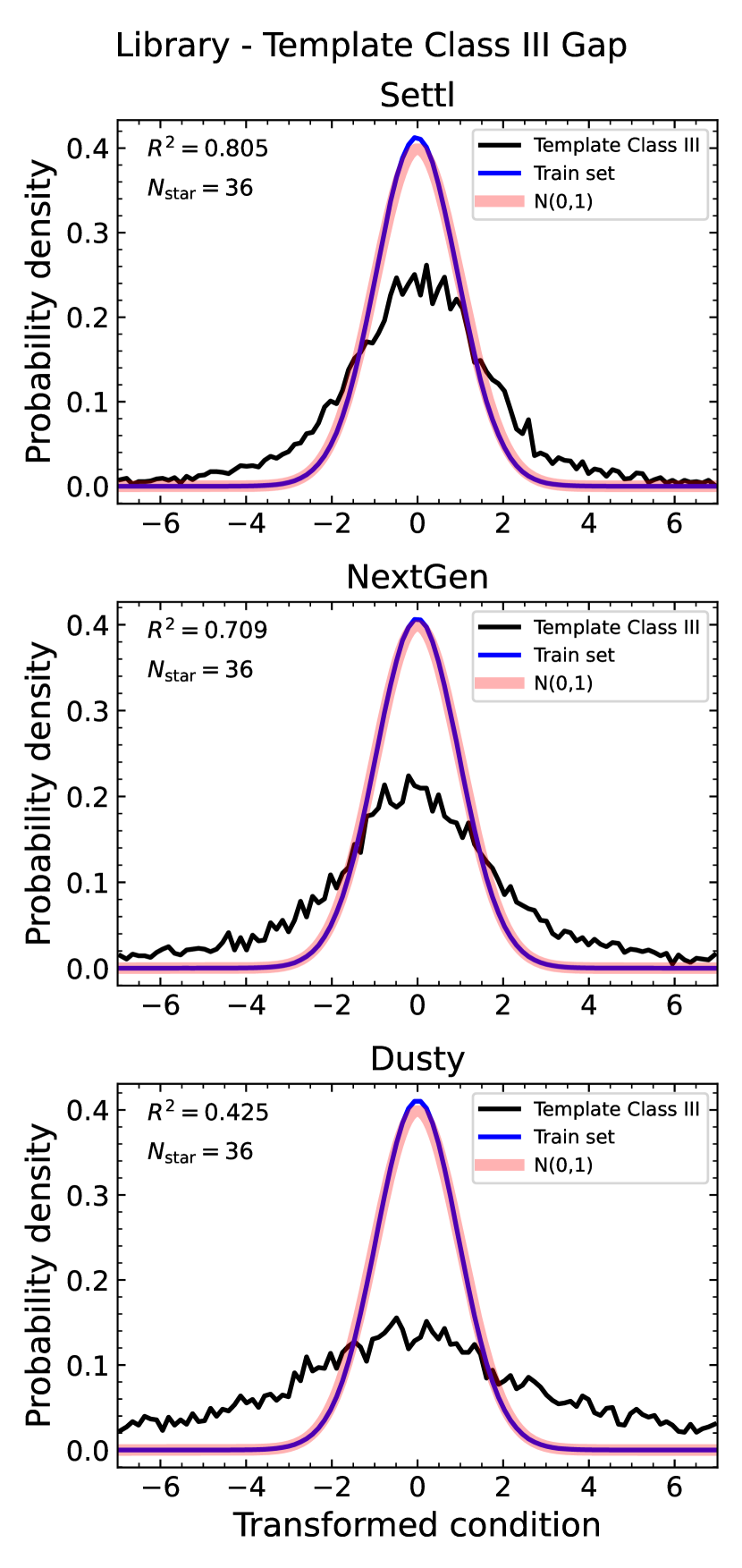
Figure 11: Probability distributions of transformed conditions of the training data (blue) and template stars (black) for three networks. The gap between the blue and black lines means the gap between the Phoenix model and the template spectrum. The $R^{2}$ value between the blue and black line and the number of template stars used are presented in the upper left corner of each panel.

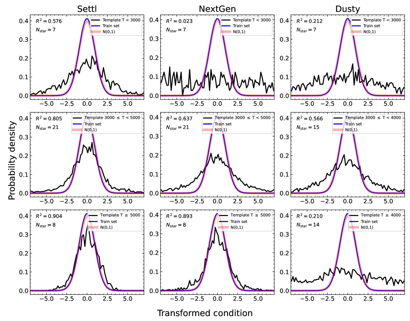
Figure 12: Probability distributions of transformed conditions of the training data and template stars. Each column represents three networks (Settl-Net, NextGen-Net, and Dusty-Net) and each row represents the group of template stars depending on their temperature ($T^{\mathrm{lit}}_{\mathrm{eff}}$). Colour codes are the same as in Fig. 11.

We trained transformation networks ($k$) for each cINNs (Settl-Net, NextGen-Net, and Dusty-Net) and compare the probability distribution of the transformed conditions of the training data and template stars. Figure 11 shows that the distribution of the training data (blue line) well follows the prescribed standard normal distribution (pink line) but the distribution of template stars (black) differs from that of the training data. There are 256 condition components for each star, but we present all these components in one distribution. The $R^{2}$ scores for all template stars are 0.805, 0.709, and 0.425 for Settl, NextGen, and Dusty, respectively. The dusty model seems to have the widest simulation gap, but we need to consider that Dusty-Net has a narrower training range than the parameter space of the template stars.

As the performance of the cINN varies depending on the temperature of the template star, we divided the stars into three groups based on the prediction performance of the networks shown in section 5.2.1 (see Figs. 3 and 4). For example, Settl-Net and NextGen-Net predicted parameters with good agreement with literature values, especially for stars with temperatures between $\sim$3000 K and $\sim$5000 K. So we divided the stars into 3 groups based on 3000 K and 5000 K for Settl-Net and NextGen-Net. In the case of Dusty-Net, due to the temperature upper limit of 4000 K for the Dusty training set, we divided groups based on 3000 K and 4000 K.

In the case of Settl and NextGen libraries (Fig. 12), the earlier the spectral type, the smaller the gap and Settl has a smaller gap than NextGen in the overall temperature range. While the simulation gap is small for hot stars above 3000 K, the gap is large for later-type stars below 3000 K. In the case of NextGen, in particular, the simulation gap is very large for stars below 3000 K. In the case of Dusty, the simulation gap for the coldest group ($T<3000$ K) is also very large and comparable to that for hot stars ($T>4000$ K), out of the temperature range of the Dusty library.

The large gap for the lowest temperature group ($T<3000$ K) is an obvious result because perfectly implementing the atmosphere of late-type stars through the simulation is a much more difficult task than the earlier type stars. For late-type stars, condensation of vapour is important but the relevant physical processes are complex, making it very difficult to produce a good atmosphere model. Thus, these results demonstrate the inherent limitations of modelling low-temperature stars. These results show that the degree of simulation gap varies with the characteristics of the star, just as the difference between the prediction of cINN and the literature value varies, as shown in section 5.2.1.

Interestingly, both Settl and NextGen have the smallest simulation gaps for the early-type stars with temperatures above 5000 K. However, in Figs. 3 and 4, the difference between the MAP prediction and the literature value of this group is slightly larger than that of the intermediate temperature group (3000–5000 K). The smallest simulation gap (Fig. 12) and good resimulation results better than the resimulation of literature values (Fig. 16 and Table 6) imply that MAP estimates of our networks for early-type stars above 5000 K are sufficiently reliable. Therefore, we suggest that the parameter estimations by our networks may be more accurate than the literature values for early-type stars above 5000 K.

7.3 Best network

It is clear that the simulation gap is large for late-type stars. Interestingly, however, our cINNs nevertheless predict the temperature and surface gravity well. First of all, all three networks had poor predictions of extinction for late-type stars below 3000 K. It is therefore very difficult for the network to estimate extinction accurately for stars in this temperature range, and the estimated extinction is not very reliable compared to the other two stellar parameters. However, Settl-Net, NextGen-Net, and Dusty-Net estimated the temperature accurately with maximum errors of less than 10, 5, and 15 per cent, respectively, despite the large simulation gap. This is a sufficiently accurate prediction considering the temperature interval between 1 subclass of stellar spectral type (see Fig. 3). Using combined error in Fig. 4, we demonstrated that Dusty-Net and Settl-Net predict surface gravity and temperature accurately within 5 per cent for late-type stars as well as early-type stars, despite the simulation gap of late-type stars. This shows that our networks are still applicable to low-temperature stars despite the limitations of training data. In the case of NextGen-Net, its performance was relatively poor for low-temperature stars compared to the other two networks, which is explained by the large simulation gap shown in Fig. 12.

On the other hand, for earlier type stars with relatively small simulation gaps, the network performs more reliably. Except for one or two outliers, both Settl-Net and NextGen-Net accurately predict temperature and gravity within a maximum error of 5 to 10 per cent. NextGen-Net tends to estimate extinction and temperature slightly higher than Settl-Net. This seems that NextGen-Net is adopting a degenerate solution that satisfies the same input spectrum by increasing both extinction and temperature slightly. Overall, Settl-Net, with the smallest simulation gap, shows the best performance among the three networks.

We conclude that Settl-Net is the best network considering both parameter prediction performance and simulation gap. Against low-temperature stars (e.g. M-type stars), Dusty-Net also shows comparable performance to Settl-Net. However, given that the stellar parameter coverage (i.e. temperature and gravity) of Settl-Net is wider than that of Dusty-Net, Settl-Net is more versatile and usable. Therefore, based on our overall results, we recommend using Settl-Net when applying the network to real observations. The only limitation to be cautious of is the estimation of extinction. Regardless of the spectral type of the stars, cINN estimates temperature and gravity accurately, but it should be cautious of using estimated extinction when the estimated temperature is below 3000 K.

8 Summary

In this paper, we introduce a novel tool to estimate stellar parameters from the optical spectrum of an individual young, low-mass star. cINN is one of the deep learning architectures specialised in solving a degenerate inverse problem. The degenerate problem here means that, due to the inevitable information loss during the forward process from the physical system to observation, different physical systems are mapped onto similar or almost identical observations. Many of the major tasks in astrophysics are solving degenerate inverse problems like estimating physical properties from observations. In this work, we develop a cINN for young low-mass stars to efficiently diagnose their optical spectra and estimate stellar parameters such as effective temperature, surface gravity, and extinction.

cINN adopts a supervised learning approach, meaning that the network is trained on the database consisting of numerous well-labelled data sets of physical parameters and observations. However, it is difficult to collect a sufficient number of well-interpreted observations in real. Therefore, we use synthetic observations instead to generate enough training data. In this work, we utilise three Phoenix stellar atmosphere libraries (i.e. Settl, NextGen, and Dusty) to produce the database for training and evaluation of the network. Interpolating the spectrum on the temperature – gravity space and adding the extinction effect on the synthetic spectra, we produce a database for each Phoenix library consisting of 65,536 synthetic models. To produce databases, we randomly sampled three parameters from the given parameter ranges. Settl and NextGen databases cover the temperature range of 2600–7000 K and $\log(g/\mathrm{cm\,s}^{-2})$ range of 2.5–5. In the case of the Dusty database, it covers the temperature of 2600–4000 K and $\log(g/\mathrm{cm\,s}^{-2})$ of 3–5. All three databases have extinction values within 0–10 mag. Then, we build and train cINNs using each database but only use 80% of the synthetic models in the database to train the network and remain the rest for evaluation. In this paper, we present three cINNs that learned about different Phoenix atmosphere models: Settl-Net, NextGen-Net, and Dusty-Net.

We validated the performance of our cINNs in various methods. Our main results are the following:

1. All three networks provide perfect predictions on the test set with the RMSE of less than 0.01 dex for all three parameters, demonstrating that the cINNs are well-trained. Additionally, we resimulate the spectrum using the parameters estimated by the network using our interpolation method and compare it with the original input spectrum. The resimulated spectra perfectly match the input spectra of the test models with RMSE of about $10^{-7}$. These results prove that our three cINNs perfectly learned the hidden rules in each training data.

2. To test the performance on the real observational data, we analyse 36 Class III template stars well-interpreted by Manara et al. (2013, 2017); Stelzer et al. (2013) with our cINNs. We demonstrate that stellar parameters estimated by our cINNs are in good agreement with the literature values.

3. Each network has a slightly different error depending on the temperature of the given star. Settl-Net works especially well for M6.5 – K1.0 (2935 – 5000 K) stars and NextGen-Net works well for M4.5 – K1.0 (3200 – 5000 K) stars. Dusty-Net works well for M5.5 – M0.0 (3060 – 4000 K) stars. Given that the temperature upper limit of Dusty training data is 4000 K, Dusty-Net works well for stars within its training range. For stars in other temperature ranges, three networks perform well with an error of less than 10 per cent.

4. The most difficult parameter for cINNs to predict is the extinction of cold stars with temperatures less than 3200 K. All three networks tend to estimate extinction higher than the literature value for cold stars. However, cINNs estimate extinction well for hot stars with temperatures above 3200 K.

5. We resimulate spectra based on cINN estimations and literature values and compare them with the original input spectrum. Interestingly, most of the resimulated spectra based on cINN estimations are closer to the input spectra than the resimulated spectra derived from literature values. This implies that our cINNs well understand the physics in each Phoenix library and are able to find the best-fitting Phoenix model (i.e. parameters) for the given observation.

6. Results that the resimulations are perfect even though the prediction of the network is slightly different from the literature can be explained by a gap between the Phoenix model and reality, so-called the simulation gap. We quantify the simulation gap between each library and template stars using the conditioning networks included in our cINNs. We confirm that the simulation gaps are relatively large for cold stars below 3000 K where the cINNs have difficulty estimating extinction. We confirm that the simulation gap is small for hot stars where cINNs predict parameters well.

7. The overall results imply that although there is an obvious gap between the Phoenix model and reality, especially for cold stars below 3000 K, our networks can nonetheless provide reliable predictions for all stars within 5–10 per cent error, especially for temperature and gravity. Extinction estimated by cINN is also reliable unless the estimated temperature is less than 3200 K.

8. We investigate which parts of the spectrum cINN relies mostly upon to predict stellar parameters and compare the important features with typically used stellar parameter tracers. We find that cINN relies on different features depending on the physical parameters and on the input observations (e.g. spectral types). We confirm that the major features are equivalent to the typically used tracers such as H$\mathrm{\alpha}$ $6563$ Å and Na i doublet $8183$, $8195$ Å.

Our overall results show that our cINNs present reliable enough performance applicable to real observational data. Among the three networks introduced in this paper, we recommend Settl-Net trained on the Settl library as the best network because of its remarkable performance and versatility on the parameter space.

Appendix A Supplemental materials

In this appendix, we present supplementary figures and table mentioned in our main results (sections 5–6).

A.1 Prediction performance

We evaluate the performance of three networks (Settl-Net, NextGen-Net, and Dusty-Net) on 13,107 synthetic test models drawn from the corresponding database by comparing the MAP predictions from the network and the true values of the models. Here, we present the result of Settl-Net in Fig. 13 as a representative because the other two networks (NextGen-Net and Dusty-Net) also show very similar results. The figure shows that the network estimates all three parameters perfectly with very small RMSEs.

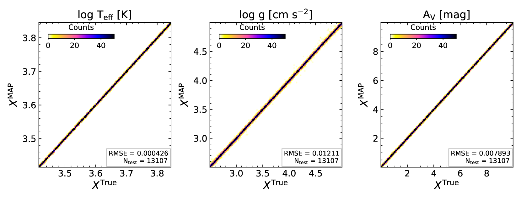
Figure 13: 2-dimensional histograms comparing the MAP values estimated by the Settl-Net and the true values for the entire test models of the Settl database. The colours indicate the number of models at each point in the 2D histograms. In the lower right corner, we present the root mean square error (RMSE) and the number of test models used (N_test).

A.2 Resimulation

We validate the cINN predictions on both the synthetic test data (Sect. 5.1.2) and real template spectra (Sect. 5.2.2) by resimulating the spectra corresponding to the MAP estimates with our spectral library interpolator (Sect. 3.1) and comparing the result to the respective input spectra.

Analogous to Fig. 1, Figs. 14 and 15 show the median relative error of the resimulated spectra (left panel) and distributions of the RMSEs (right panel) for the 13,107 synthetic test spectra when evaluated with the cINN models trained on NextGen and Dusty, respectively.

Table 6 provides a summary of the resimulation results for the cINN predictions on the Class III template spectra (see Sect. 5.2.2 and also Tables 1 and 4). Here we list the RMSEs and $R^{2}$ scores of the resimulated spectra with respect to the corresponding input spectra for the resimulation based on the literature and cINN-predicted parameters for all three spectral libraries.

Figures 16 and 17 provide additional examples of the resimulation results, comparing the resimulated spectra to the input spectra and the outcomes between the three libraries, analogous to Fig. 5. In particular, these two Figs. show examples, where the resimulated spectra based on the cINN MAP estimates seem to match the input spectra notably better than the respective resimulation outcome based on the literature properties of the given Class III templates.

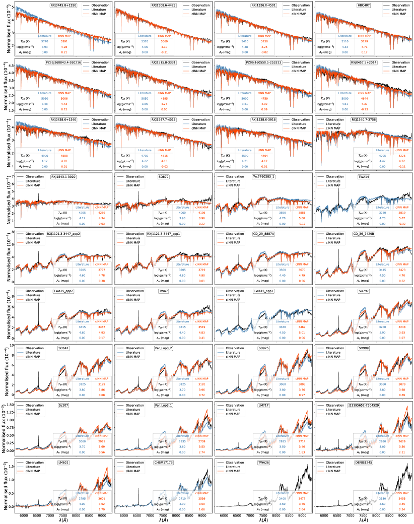
Figure 18: Resimulation results for all Class III templates for the cINN trained on the Settl library. In each panel, the black curve indicates the observed spectrum, while the red and blue curves correspond to the spectra resimulated based on the cINN MAP estimates and literature properties, respectively. The latter values are summarised in the table in each panel. Note that if either the red or blue or both curves are missing that the corresponding set of parameters could not be resimulated. For the RMSEs and $R^{2}$ scores of the resimulated spectra see Table 6.

Lastly, Fig. 18 provides an overview of the resimulation results for all Class III template spectra for the cINN trained on the Settl library, corresponding to the top left panels in Figs. 5, 16 and 17.

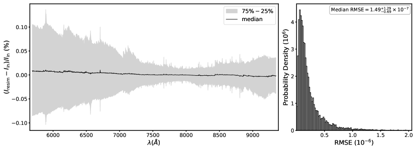
Figure 14: Resimulation results of NextGen-Net for the entire synthetic spectra in the test set. Left: Median relative error across the wavelength range of the resimulated spectra based on the MAP predictions of the cINN trained on the NextGen models averaged over the 13,107 synthetic spectra in the test set. Here the grey envelope indicates the interquantile range between the $25\%$ and $75\%$ quantiles. Right: Histogram of the RMSEs of the 13,107 resimulated spectra. The mean resimulation RMSE across the test set is $2.28\pm 2.48\times 10^{-7}$.

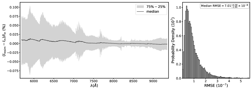
Figure 15: Resimulation results of Dusty-Net for the entire synthetic spectra in the test set. Left: Median relative error across the wavelength range of the resimulated spectra based on the MAP predictions of the cINN trained on the Dusty models averaged over the 13,107 synthetic spectra in the test set. Here the grey envelope indicates the interquantile range between the $25\%$ and $75\%$ quantiles. Right: Histogram of the RMSEs of the 13,107 resimulated spectra. The mean resimulation RMSE across the test set is $9.01\pm 7.34\times 10^{-8}$.

Table 6: Summary of the resimulation test for the literature values and cINN MAP predictions for the three different spectral libraries, listing the RMSEs and $R^{2}$ scores of the resimulated spectra.

	Resimulation RMSE ($\times 10^{-5}$) / $R^{2}$ Score
	Settl			NextGen			Dusty
Object Name	Literature	cINN	Comment	Literature	cINN	Comment	Literature	cINN	Comment
RXJ0445.8+1556	2.15 / 0.88	0.61 / 0.99	-	2.18 / 0.88	0.77 / 0.98	-	- / -	- / -	$T_{\mathrm{eff}}>4000$ K
RXJ1508.6-4423	0.95 / 0.98	0.93 / 0.98	-	1.08 / 0.98	1.05 / 0.98	-	- / -	- / -	$T_{\mathrm{eff}}>4000$ K
RXJ1526.0-4501	1.14 / 0.97	0.66 / 0.99	-	1.20 / 0.96	0.77 / 0.98	-	- / -	- / -	$T_{\mathrm{eff}}>4000$ K
HBC407	1.00 / 0.97	0.68 / 0.99	-	1.16 / 0.96	0.91 / 0.97	-	- / -	- / -	$T_{\mathrm{eff}}>4000$ K
PZ99J160843.4-260216	1.08 / 0.96	0.82 / 0.98	-	1.19 / 0.95	0.93 / 0.97	-	- / -	- / -	$T_{\mathrm{eff}}>4000$ K
RXJ1515.8-3331	1.28 / 0.94	0.85 / 0.97	-	1.41 / 0.92	0.92 / 0.97	-	- / -	- / -	$T_{\mathrm{eff}}>4000$ K
PZ99J160550.5-253313	1.50 / 0.90	0.73 / 0.98	-	1.64 / 0.88	0.93 / 0.96	-	- / -	- / -	$T_{\mathrm{eff}}>4000$ K
RXJ0457.5+2014	1.98 / 0.78	1.23 / 0.92	-	2.07 / 0.76	1.25 / 0.91	-	- / -	- / -	$T_{\mathrm{eff}}>4000$ K
RXJ0438.6+1546	2.09 / 0.70	0.89 / 0.95	-	2.19 / 0.67	1.02 / 0.93	-	- / -	- / -	$T_{\mathrm{eff}}>4000$ K
RXJ1547.7-4018	0.90 / 0.97	0.95 / 0.96	-	1.08 / 0.95	1.11 / 0.95	-	- / -	- / -	$T_{\mathrm{eff}}>4000$ K
RXJ1538.6-3916	1.05 / 0.93	0.92 / 0.94	-	1.24 / 0.90	1.20 / 0.91	-	- / -	- / -	$T_{\mathrm{eff}}>4000$ K
RXJ1540.7-3756	1.42 / 0.56	1.61 / 0.44	-	1.56 / 0.48	1.54 / 0.49	-	- / -	- / -	$T_{\mathrm{eff}}>4000$ K
RXJ1543.1-3920	1.48 / 0.42	1.63 / 0.30	-	1.72 / 0.22	1.48 / 0.42	-	- / -	- / -	$T_{\mathrm{eff}}>4000$ K
SO879	2.66 / 0.53	2.44 / 0.61	-	3.02 / 0.39	2.18 / 0.68	-	- / -	2.08 / 0.71	-
Tyc7760283_1	2.56 / 0.73	1.88 / 0.85	-	1.99 / 0.84	1.95 / 0.84	-	1.93 / 0.85	1.89 / 0.85	$5<\log(g)<5.5$
TWA14	3.04 / 0.83	- / -	$\log(g)>5$	3.28 / 0.80	2.74 / 0.86	-	2.96 / 0.84	3.07 / 0.82	$5<\log(g)<5.5$
RXJ1121.3-3447_app2	2.19 / 0.93	1.88 / 0.95	-	2.45 / 0.91	2.15 / 0.93	-	1.86 / 0.95	1.80 / 0.95	$5<\log(g)<5.5$
RXJ1121.3-3447_app1	2.69 / 0.92	2.84 / 0.91	-	3.60 / 0.85	2.44 / 0.93	-	2.87 / 0.91	2.42 / 0.93	$5<\log(g)<5.5$
CD_29_8887A	2.55 / 0.95	1.91 / 0.97	-	2.57 / 0.95	2.48 / 0.95	-	1.92 / 0.97	1.85 / 0.97	$5<\log(g)<5.5$
CD_36_7429B	2.70 / 0.97	2.30 / 0.98	-	4.90 / 0.91	2.57 / 0.97	-	3.26 / 0.96	2.26 / 0.98	-
TWA15_app2	2.98 / 0.96	3.04 / 0.96	-	4.04 / 0.92	2.59 / 0.97	-	2.93 / 0.96	2.57 / 0.97	$5<\log(g)<5.5$
TWA7	3.45 / 0.95	3.62 / 0.94	-	4.53 / 0.91	2.66 / 0.97	-	3.36 / 0.95	2.76 / 0.97	-
TWA15_app1	3.95 / 0.93	- / -	$\log(g)>5$	3.26 / 0.95	2.95 / 0.96	-	3.01 / 0.96	2.96 / 0.96	$5<\log(g)<5.5$
SO797	3.77 / 0.97	2.70 / 0.98	-	6.35 / 0.92	2.47 / 0.99	-	4.63 / 0.96	2.27 / 0.99	-
SO641	3.83 / 0.97	3.15 / 0.98	-	6.37 / 0.92	2.62 / 0.99	-	4.76 / 0.96	2.63 / 0.99	-
Par_Lup3_2	3.68 / 0.97	3.03 / 0.98	-	4.74 / 0.95	2.86 / 0.98	-	3.31 / 0.98	2.76 / 0.98	-
SO925	4.55 / 0.97	4.42 / 0.97	-	7.28 / 0.91	3.06 / 0.98	-	5.91 / 0.94	3.17 / 0.98	-
SO999	4.20 / 0.97	3.90 / 0.97	-	6.27 / 0.93	2.99 / 0.98	-	5.00 / 0.96	3.10 / 0.98	-
Sz107	4.44 / 0.97	4.85 / 0.96	-	6.58 / 0.93	2.83 / 0.99	-	5.32 / 0.95	3.11 / 0.98	-
Par_Lup3_1	8.90 / 0.92	5.64 / 0.97	-	12.4 / 0.85	- / -	$\log(g)<2.5$	11.5 / 0.87	4.05 / 0.98	-
LM717	7.08 / 0.95	5.77 / 0.96	-	10.1 / 0.88	- / -	$\log(g)<2.5$	9.80 / 0.90	- / -	$\log(g)<3.0$
J11195652-7504529	7.49 / 0.95	6.73 / 0.96	-	10.9 / 0.89	- / -	$\log(g)<2.5$	10.1 / 0.89	- / -	$\log(g)<3.0$
LM601	7.76 / 0.94	7.26 / 0.95	-	9.97 / 0.91	- / -	$\log(g)<2.5$	9.06 / 0.92	- / -	$\log(g)<3.0$
CHSM17173	8.65 / 0.94	- / -	$T_{\mathrm{eff}}<2700$ K	10.1 / 0.90	- / -	$\log(g)<2.5$	9.63 / 0.92	- / -	$\log(g)<3.0$
TWA26	- / -	- / -	$T_{\mathrm{eff}}<2700$ K	- / -	- / -	$\log(g)<2.5$	- / -	- / -	$T_{\mathrm{eff}}<2700$ K
DENIS1245	- / -	- / -	$T_{\mathrm{eff}}<2700$ K	- / -	- / -	$\log(g)<2.5$	- / -	- / -	$T_{\mathrm{eff}}<2700$ K
Resimulated Spectra	34	31	-	34	29	-	20	17	-

A.3 Feature importance

We investigate the important feature where NextGen-Net and Dusty-Net rely mostly upon. We divided the synthetic observations into three groups depending on their spectral types (e.g. M-, K-, and G-types). We present the results of NextGen-Net and Dusty-Net for M-type stars in Fig. 19. We do not present the results of NextGen-Net for K- and G-type stars because overall results are similar to that of Settl-Net presented in Fig. 10.

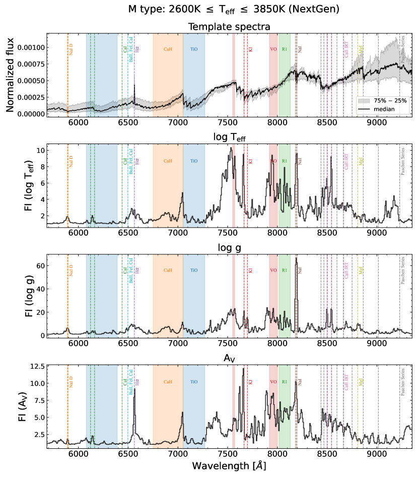
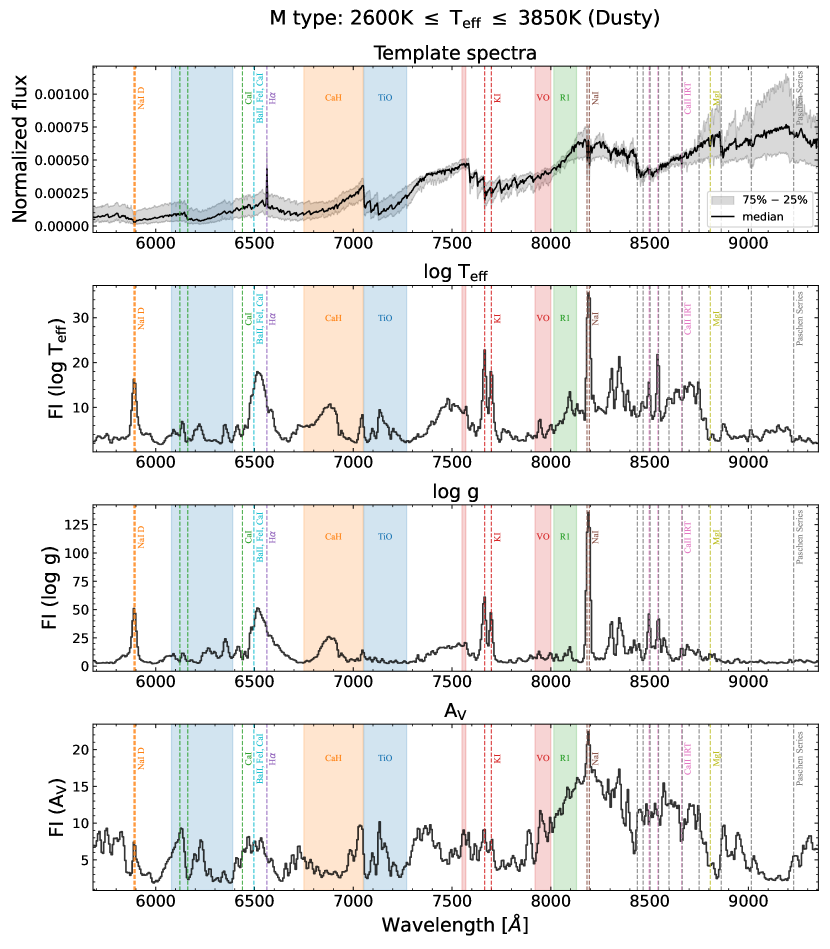
Figure 19: Feature importance evaluation for M-type synthetic models in the test set using NextGen-Net (left) and Dusty-Net (right), respectively. The first row shows the median flux of M-type Class III template stars. Lines and shades are the same as Fig. 9.