Beyond first-order methods for non-convex non-concave min-max optimization

Abstract

We propose a study of structured non-convex non-concave min-max problems which goes beyond standard first-order approaches. Inspired by the tight understanding established in recent works (Adil et al., 2022; Lin and Jordan, 2022b), we develop a suite of higher-order methods which show the improvements attainable beyond the monotone and Minty condition settings. Specifically, we provide a new understanding of the use of discrete-time $p^{th}$-order methods for operator norm minimization in the min-max setting, establishing an $O(1/\epsilon^{\frac{2}{p}})$ rate to achieve $\epsilon$-approximate stationarity, under the weakened Minty variational inequality condition of Diakonikolas et al. (2021). We further present a continuous-time analysis alongside rates which match those for the discrete-time setting, and our empirical results highlight the practical benefits of our approach over first-order methods.

1 Introduction

In this work we study the classic min-max problem:

$$\min_{x\in\mathcal{X}}\max_{y\in\mathcal{Y}}f(x,y),$$ (1.1)

whereby $f:\mathcal{X}\times\mathcal{Y}\mapsto\mathbb{R}$ may be non-convex in $x$ and non-concave in $y$, and where we assume $f$ is smooth (up to various orders) in both $x$ and $y$. Problems of this form naturally arise in many different areas of machine learning, from training generative adversarial networks (Goodfellow et al., 2020), to adversarial training/robustness (Madry et al., 2018; Zhang et al., 2019), along with more general robust optimization objectives (Ben-Tal et al., 2009).

In the case where $f$ is smooth and convex-concave in $x$ and $y$, respectively, algorithms such as the extragradient method (Korpelevich, 1976) and its generalizations such as Mirror Prox (Nemirovski, 2004) are able to converge (in terms of duality gap) at a rate of $O(1/\epsilon)$, and this is known to be tight for first-order methods (Ouyang and Xu, 2021). However, as the complexity (and inherent non-convexity) of the underlying models for these large-scale problems increases, so too does the need to expand beyond the convex-concave setting.

Unfortunately, in the most general constrained non-convex non-concave setting, it would appear there is not much hope for efficiently finding a stationary point, as even doing so approximately has been shown to be FNP-complete (Daskalakis et al., 2021). Recently, however, there has been significant interest in overcoming these difficulties by looking instead at certain structured non-convex non-concave problems. Specifically, we take inspiration from the previous work by Diakonikolas et al. (2021), which, for the more general case of variational inequalities, establishes a useful characterization of problems defined in terms of a weakening of the standard Minty condition. Diakonikolas et al. (2021) further provide a generalization of the extragradient method, which they show manages to reach an $\epsilon$-approximate stationary point (w.r.t. the norm of the operator) at a $O(1/\epsilon^{2})$ rate. In addition, by choosing the operator $F=[\nabla_{x}f,-\nabla_{y}f]^{\top}$, they establish the same rate for reaching stationary points of the unconstrained min-max optimization problem, under their weak-MVI condition (which is weaker than assuming the variational inequality satisfies the Minty condition (Song et al., 2020; Lin and Jordan, 2022b)), and they further show how their results may extend to non-Euclidean settings.

Building on these efforts, we aim to understand the opportunities afforded by going beyond the standard first-order extragradient approach. In particular, recent works (Adil et al., 2022; Lin and Jordan, 2022b) have presented optimal $p^{th}$-order methods for approximately solving monotone variational inequalities. In this work, we show how to relax this monotonicity condition, in a similar manner to that of Diakonikolas et al. (2021), that is suitable to a variant of the higher-order extragradient method.

1.1 Our Contributions

Our main contributions are as follows.

• We propose the hoeg+ method, based on a higher-order variant (Adil et al., 2022) of the extragradient algorithm (Korpelevich, 1976), and we establish convergence results for structured non-convex non-concave min-max problems.

• For a generalized weak-MVI condition inspired by (Diakonikolas et al., 2021), we show that the $p^{th}$-order instance of our algorithm finds $\epsilon$-approximate stationary points at a $O(1/\epsilon^{\frac{2}{p}})$ rate. Furthermore, these are to our knowledge the first results that go beyond the $O(1/\epsilon^{2})$ rate for the weak-MVI setting.

• In the continuous-time regime, we show that the algorithm achieves an analogous rate of $\min_{0\leq t\leq T}\|F(z_{t})\|\leq O(1/T^{\frac{p}{2}})$ under the weak-MVI condition. Furthermore, under the co-monotonicity condition on the operator which implies weak-MVI, the first-order instance of the algorithm has $\|F(z(t))\|$ decreasing and thus $\|F(z(t))\|\leq O(1/\sqrt{t})$.

• We provide a study of the empirical performance of the first- and second-order instances of our algorithm based on weak-MVI examples with the standard min-max operator $F=(\nabla_{x}f,-\nabla_{y}f)$, as well as the competitive operator $F_{\alpha}$ introduced in (Vyas and Azizzadenesheli, 2022).

Algorithm
(Reference)	Bounded range ($\alpha\leq f(x)\leq\beta\ \forall x\in\mathbb{R}^{n}$)			General operator?
	$p=1$	$p=2$	$p>2$
Gradient Descent
(Folklore)	$O\left(1/\epsilon^{2}\right)$	—	—	No
Cubic Regularization
(Nesterov and Polyak, 2006)	—	$O\left(1/\epsilon^{\frac{3}{2}}\right)$	—	No
AR$p$ (Birgin et al., 2017)	$O\left(1/\epsilon^{2}\right)$	$O\left(1/\epsilon^{\frac{3}{2}}\right)$	$O\left(1/\epsilon^{\frac{p+1}{p}}\right)$	No
	$p^{th}$-Order weak-MVI (Assumption 1)
	$p=1$	$p=2$	$p>2$
Extragradient+
(Diakonikolas et al., 2021)	$O(1/\epsilon^{2})$	—	—	Yes
hoeg+ (Algorithm 1)
Theorem 3.5 (This Paper)	$O(1/\epsilon^{2})$	$O(1/\epsilon)$	$O(1/\epsilon^{\frac{2}{p}})$	Yes

Table 1: Discrete-time convergence rates for reaching $\epsilon$-approximate stationary points in the unconstrained Euclidean setting, under bounded range and $p^{th}$-order weak-MVI assumptions, respectively, in addition to $p^{th}$-order smoothness. Note that for $p=1$, the weak-MVI assumption leads to the same rate as in the standard (bounded range) non-convex setting, whereas our method highlights the improvements attainable when going beyond first-order methods, for $p>1$.

	Monotone	$p^{th}$-Order weak-MVI (Assumption 1)
Algorithm 2 in (Lin and Jordan, 2022a)
Theorem 4.1	$O(1/\epsilon^{\frac{2}{p}})$	—
hoeg+(Algorithm 1)
Theorem 3.1 (This Paper)	$O(1/\epsilon^{\frac{2}{p}})$	$O(1/\epsilon^{\frac{2}{p}})$

Table 2: Continuous-time convergence rates for reaching $\epsilon$-approximate stationary points in the unconstrained Euclidean setting, under monotonicity and $p^{th}$-order weak-MVI assumptions, in addition to $p^{th}$-order smoothness.

1.2 Additional Related Works

Recently, several works (Bullins and Lai, 2022; Jiang and Mokhtari, 2022; Adil et al., 2022; Lin and Jordan, 2022b) have shown how to achieve $\epsilon$-approximate weak solutions to monotone variational inequalities under $p^{th}$-order oracle access, wherein the $O(1/\epsilon^{\frac{2}{p+1}})$ rates of Adil et al. (2022); Lin and Jordan (2022b) (which remove additional logarithmic factors) are optimal. However, these works have focused predominantly on the convex-concave (monotone operator) setting, though Lin and Jordan (2022b) also show a rate of $O(1/\epsilon^{\frac{2}{p}})$ under the Minty condition. In addition, Lin and Jordan (2022a) provide a rate of $O(1/\epsilon^{\frac{2}{p}})$ to reach a point with small operator norm in the monotone setting.

In more typical non-convex optimization settings, especially given the ubiquity of large-scale models for modern machine learning, much attention has been paid to developing methods which can find approximate stationary points (that is, places where $\left\lVert\nabla f(x)\right\rVert\leq\epsilon$). One such example is the cubic regularization method (Nesterov and Polyak, 2006) and its higher-order generalization (Birgin et al., 2017), providing rates that match the lower bounds (Carmon et al., 2020). Furthermore, even first-order (as well as Hessian-vector product-based) methods have also been shown to benefit from higher-order smoothness, with certain accelerated methods giving rise to even faster rates (Agarwal et al., 2017; Carmon et al., 2017, 2018; Jin et al., 2018; Li and Lin, 2022), though there remains a small gap between upper and lower bounds (Carmon et al., 2021).

The continuous-time regime has proven to be effective in analyzing the performance of algorithms for minimization problems (Latz, 2021; Wilson et al., 2016; Wibisono et al., 2016; Shi et al., 2021), min-max optimization problems (Lin and Jordan, 2022a; Vyas and Azizzadenesheli, 2022), and in the study of continuous games (Mazumdar et al., 2020). Latz (2021) analyzes stochastic gradient descent in the continuous-time regime while Wilson et al. (2016); Wibisono et al. (2016); Shi et al. (2021) provide a continuous-time perspective of the accelerated variants of gradient descent. Lin and Jordan (2022a) study the continuous-time version of the dual-extrapolation algorithm, and Vyas and Azizzadenesheli (2022) build on the competitive gradient descent algorithm (Schäfer and Anandkumar, 2019) to design a new min-max algorithm based on re-scaling the cross-terms of the Jacobian of the operator.

2 Preliminaries

In this section we discuss the notations and key assumptions that formulate the setting for our algorithm. We start by defining the approximate and exact stationary points of an operator $F$.

Definition 2.1 (Stationary points).

A point $z\in\mathcal{Z}\subseteq\mathbb{R}^{d}$, is an $\epsilon$-approximate stationary point if

$$\|F(z)\|\leq\epsilon,$$

and it is an exact stationary point if

$$\|F(z)\|=0.$$

We then define the solution set to the Stampachchia variational inequality for any field $F$.

Definition 2.2 (Solution set $\mathcal{Z}^{*}$).

We refer to the solutions of the Stampachchia Variational Inequality (SVI):

$$\langle F(z^{*}),z-z^{*}\rangle\geq 0$$

as the set $\mathcal{Z}^{*}\subseteq\mathcal{Z}$.

To solve the problem in Eq. (1.1) we consider the field $F=\begin{bmatrix}\nabla_{x}f\\ -\nabla_{y}f\end{bmatrix}$, derived from the function $f$. For the unconstrained setting, i.e, $\mathcal{Z}=\mathbb{R}^{d}$, we have $\|F(z^{*})\|=0~{}\forall z^{*}\in\mathcal{Z}^{*}$. Furthermore all stationary points of Eq.(1.1) satisfy the SVI. We assume $\mathcal{Z}^{*}\neq\phi$.

We start by defining the monotonicity of an operator.

Definition 2.3 (Monotonicity).

An operator is monotone if for all $z_{a},z_{b}\in\mathcal{Z}$,

$$\langle F(z_{a})-F(z_{b}),z_{a}-z_{b}\rangle\geq 0$$

Standard examples of monotone operators include the gradient $\nabla f$ of a convex function $f(x)$ and the concatenated gradient $(\nabla_{x}f,-\nabla_{y}f)$ for a convex-concave $f(x,y)$ function.

We now present the definition of comonotonicity condition which generalizes monotonicity. This was used as the key non-monotone condition to provide first-order algorithms in Lee and Kim (2021).

Definition 2.4 ($\rho$-comonotone).

An operator $F$ is $\rho$-comonotone if,

$$\langle F(z_{a})-F(z_{b}),z_{a}-z_{b}\rangle>\rho\|F(z_{a})-F(z_{b})\|~{}\forall z_{a},z_{b}\in\mathcal{Z}$$

Note that for $\rho$-comonotonicity implies monotonicity for $\rho\geq 0$.

Inspired by the weak-MVI condition in Diakonikolas et al. (2021) we generalise to the weak-MVI condition to $p$-dimensions. This condition is the key condition under which we prove the convergence of our algorithm.

Assumption 1 ($p^{th}$-Order weak-mvi).

There exists $z^{*}\in\mathcal{Z}^{*}$ such that:

$$(\forall z\in\mathbb{R}^{d}):\quad\left\langle F(z),z-z^{*}\right\rangle\geq-\frac{\rho}{2}\|F(z)\|^{\frac{p+1}{p}},$$ (a₁)

for some parameter $\rho\geq 0$.

For $\rho=0$ the condition is the well-known MVI condition Mertikopoulos et al. (2018). Furthermore for $p=1$, $\rho$-comonotonicity implies $-\frac{\rho}{2}$ weak-MVI. Overall, monotonicity implies MVI which implies weak-MVI.

Finally we define the smoothness of an operator.

Assumption 2 ($p^{th}$-Order Smoothness).

$$\|F(z_{b})-\tau_{p-1}(z_{b},z_{a})\|\leq\frac{L_{p}}{p!}\|z_{b}-z_{a}\|^{p},\forall z_{a},z_{b}\in\mathcal{Z}$$ (a₂)

We now define some quantities used in the algorithm.

Definition 2.5.

We define $\tau_{p}$ as the Taylor approximation of $F$ at $z_{b}$ centered at $z_{a}$,

$$\tau_{p}(z_{a},z_{b}):=\sum_{i=0}^{p}\nabla^{i}F(z_{a})[z_{b}-z_{a}]^{i}$$ (2.1)

Definition 2.6.

We define $\Phi_{p}$ as the regularized Taylor approximation,

$$\Phi_{p}(z_{b},z_{a}):=\tau_{p-1}(z_{b},z_{a})+\frac{2L_{p}}{p!}\|z_{b}-z_{a}\|^{p-1}(z_{b}-z_{a}).$$ (2.2)

3 Convergence Results

In this section we will present our algorithm and discuss in detail the conditions under which it converges to stationary points. we will start by analysing the behaviour of the algorithm under the limit of the learning rate approaching zero. Under the said limit the algorithm can be represented as a dynamical system, and we will analyze the system which is the continuous-time analogue of our algorithm with the conditions of weak-MVI and comonotonicity on the operator. We will then proceed to analyze the discrete-time algorithm under the generalized weak-MVI condition.

We now present our algorithm hoeg+, a higher-order variant of the extra-gradient method. The algorithm is as follows.

1 $z_{0}\in\mathcal{X}\times\mathcal{Y}$;

2 for k = 0 to k = K do

3       $z_{k+\frac{1}{2}}=z^{\prime}\ \textrm{s.t.}\ \Phi(z^{\prime},z_{k})=0$

4       $\lambda_{k}=\frac{1}{2}\|z_{k+\frac{1}{2}}-z_{k}\|^{1-p}$

5       $z_{k+1}=\operatorname*{argmin}_{z^{\prime\prime}\in\mathbb{R}^{d}}\Big{\{}\left\langle F(z_{k+\frac{1}{2}}),z^{\prime\prime}-z_{k+\frac{1}{2}}\right\rangle+\frac{L_{p}}{p!\lambda_{k}}\|z_{k}^{\prime\prime}-z_{k}\|^{2}\Big{\}}$= $z_{k}-\frac{p!\lambda_{k}}{2L_{p}}F(z_{k+\frac{1}{2}})$

return $z_{out}=\operatorname*{argmin}_{z_{k+\frac{1}{2}},0\leq k\leq K}\|z_{k+\frac{1}{2}}\|$

Algorithm 1 hoeg+

We now discuss the convergence of the dynamics of the system of differential equations obtained in the limit of the higher-order extra-gradient method. The continuous-time dynamics of the $p^{th}$-order dual extrapolation algorithm (Nesterov, 2007), as given by Lin and Jordan (2022a), are

$$\begin{array}[]{lll}\dot{s}(t)=-\tfrac{F(z(t))}{\|F(z(t))\|^{1-1/p}},&v(t)=z_{0}+s(t),&z(t)-v(t)+\tfrac{F(z(t))}{\|F(z(t))\|^{1-1/p}}=\textbf{0},\end{array}$$ (3.1)

While Lin and Jordan (2022a) shows that (3.1) is the dynamical system for dual extrapolation, we know that dual extrapolation is equivalent to the extra-gradient method for the unconstrained Euclidean setting (Nesterov, 2007), and so the system of (3.1) is the continuous-time analog of hoeg+.

Theorem 3.1.

Let the operator $F$ satisfy (a₁) with $\rho<2$. Then for the continuous-time dynamics (3.1) we have $\min_{0\leq s\leq t}\|F(z(s))\|^{2}$ follows $O(\frac{1}{t^{p}})$.

Proof.

Let us consider the lyapunov function $\mathcal{E}=\|s(t)\|^{2}$.

Expanding this equality with any $z\in\mathcal{Z}$, we have

$$\frac{d\mathcal{E}(t)}{dt}=\frac{2(\langle F(z(t)),z_{0}-z\rangle+\langle F(z(t)),z-z(t)\rangle+\langle F(z(t)),z(t)-v(t)\rangle)}{\|F(z(t))\|^{1-1/p}}$$

Since $\dot{s}(t)=-\tfrac{F(z(t))}{\|F(z(t))\|^{1-1/p}}$, we have

$$\frac{\langle F(z(t)),z_{0}-z\rangle}{\|F(z(t))\|^{1-1/p}}=-\langle\dot{s}(t),z_{0}-z\rangle.$$

Since $F$ satisfies the weak-MVI assumption we have,

$$\langle F(z(t)),z-z(t)\rangle\leq\frac{\rho}{2}\|F(z(t))\|^{\frac{p+1}{p}}-\langle F(z(t)),z^{*}-z\rangle$$

Since $z(t)-v(t)+\tfrac{F(z(t))}{\|F(z(t))\|^{1-1/p}}=\textbf{0}$, we have

$$\frac{\langle F(z(t)),z(t)-v(t)\rangle}{\|F(z(t))\|^{1-1/p}}=-\|F(z(t))\|^{\frac{2}{p}}.$$

Plugging these pieces together in Eq. (3) yields that, for any $z\in\mathcal{Z}$, we have

$$\frac{d\mathcal{E}(t)}{dt} \leq 2\langle\dot{s}(t),z-z_{0}\rangle+2\langle\dot{s},z^{*}-z\rangle-(2-\rho)\|F(z(t))\|^{\frac{2}{p}}.$$ (3.2)

$$\leq 2\langle\dot{s}(t),z^{*}-z_{0}\rangle-(2-\rho)\|F(z(t))\|^{\frac{2}{p}}.$$ (3.3)

Integrating this inequality over $[0,t]$, using $\mathcal{E}(0)=0$ and observing $\langle s(t),z^{*}-z_{0}\rangle-\|s(t)\|^{2}\leq\frac{1}{4}\|z^{*}-z_{0}\|^{2}$, $\|z_{0}-z^{*}\|\leq D$, we have,

$$\int_{0}^{t}\|F(z(s))\|^{\frac{2}{p}}\;ds\leq\frac{1}{2-\rho}\left(\langle s(t),z^{*}-z_{0}\rangle-\|s(t)\|^{2}\right)\leq\frac{D^{2}}{4(2-\rho)},\quad\textnormal{for all }t\geq 0.$$

Now let $m=\min_{0\leq s\leq t}\|F(z(s))\|^{\frac{2}{p}}=(\min_{0\leq s\leq t}\|F(z(s))\|)^{\frac{2}{p}}$, where the second equality is true since $\|.\|^{\frac{2}{p}}$ is increasing for $p\geq 1$. Then we have,

$$mt\leq\int_{0}^{t}\|F(z(s))\|^{\frac{2}{p}}\;ds\leq\frac{D^{2}}{4(2-\rho)},\rightarrow\min_{0\leq s\leq t}\|F(z(s))\|^{2}\leq\frac{D^{2p}}{4(2-\rho)^{p}t^{p}}=O(\frac{1}{t^{p}})\quad\textnormal{for all }t\geq 0.$$

∎

While the weak-MVI condition with $\rho<2$ is sufficient to obtain the desired $O(\frac{1}{t^{p}})$ rates, we show that for an operator that is comonotone with $\rho>-1$ the dynamics (3.1) are such that $\|F(z(t))\|$ is decreasing furthermore since comonotonicity with $\rho>-1$ implies weak-MVI with $\rho>2$ we have the conditions of Theorem 3.1 satisfied and thus $\|F(z(t))\|=\min_{0\leq s\leq t}\|F(x(s))\|\leq O(\frac{1}{t})$.

Corollary 3.2.

If the operator $F$ is $\rho$-comonotone with $\rho>-1$, for the time dynamics (3.1) with $p=1$ we have $\|F(z(t))\|$ is decreasing and $\|F(z(t))\|^{2}$ follows $O(\frac{1}{t})$.

Proof.

Since the operator is $\rho$-comonotone with $\rho>-1$ we have

$$\langle F(z_{1})-F(z_{2}),z_{1}-z_{2}\rangle>-\|F(z_{1})-F(z_{2})\|~{}\forall z_{1},z_{2}\in\mathcal{Z}$$

Setting $z_{2}=z^{*}$ where $\|F(z^{*})\|=0$, we obtain that $F$ satsifies assumption (a₁) with $\rho<2$ and thus from Theorem 3.1 we have,

$$\min_{0\leq s\leq t}\|F(z(s))\|^{2}\leq O(\frac{1}{t})$$ (3.4)

Furthermore setting $z_{1}=z+\tau\delta z,~{}z_{2}=z$ and taking limit $\tau\rightarrow 0$ we obtain

$$\lim_{\tau\rightarrow 0}\langle F(z+\tau\delta z)-F(z),z+\tau\delta z-z\rangle>-\lim_{\tau\rightarrow 0}\|F(za+\tau\delta z)-F(z)\|^{2}$$

this gives

$$\lim_{\tau\rightarrow 0}\langle\frac{F(z+\tau\delta z)-F(z)}{\tau},\delta z\rangle>-\lim_{\tau\rightarrow 0}\|(\frac{F(z+\tau\delta z)-F(z)}{\tau})^{2}\|$$

which gives

$$\langle\nabla F(z)\delta z,\delta z\rangle+\|\nabla F(z)\delta z\|^{2}\geq 0$$ (3.5)

We now prove that $t\mapsto\|F(z(t))\|$ is non-increasing for the dynamics  (3.1). The dynamics are,

$$\dot{s}(t)=-F(z(t)),\quad v(t)=z_{0}+s(t),\quad z(t)-v(t)+F(z(t))=\textbf{0}.$$

In this case, we can write $z(t)=(I+F)^{-1}v(t)$. Since $v(\cdot)$ is continuously differentiable, we have $x(\cdot)$ is also continuously differentiable. Define the function $g(t)=\frac{1}{2}\|v(t)-z(t)\|^{2}$. Then we have,

$$\dot{g}(t)=\langle\dot{v}(t)-\dot{z}(t),v(t)-z(t)\rangle=-\langle\dot{v}(t)-\dot{z}(t),\dot{v}(t)\rangle=-\|\dot{v}(t)-\dot{z}(t)\|^{2}-\langle\dot{v}(t)-\dot{z}(t),\dot{z}(t)\rangle.$$

Now

$$\dot{v}(t)-\dot{z}(t)=\nabla F(z(t))\dot{z}(t)$$

thus choosing $z=z(t),\delta z=\dot{z}(t)$ in Eq. (3.5) we obtain,

$$\dot{g}(t)=-(\|\nabla F(z(t))\dot{z}(t)\|^{2}+\langle\nabla F(z(t))\dot{z},\dot{z}\rangle)<0$$

Thus $\|F(z(t))\|$ is decreasing and combined with (3.4) we have,

$$\|F(z(t))\|^{2}\leq O(\frac{1}{t})$$

which is the statement of the corollary. ∎

Note that $-1$-comontoncitiy is sufficient for $\|F(z(t))\|$ to be non-increasing but violates the conditions of Theorem 3.1.

3.1 Discrete Time

For discrete time we discuss the results in three different settings discussed above. We start by establishing several key lemmas, the first of which comes from Adil et al. (2022).

Lemma 3.3 (Adil et al. (2022)).

For the iterates of the Algorithm 1 $\{z_{k}\}_{k=1}^{K}$ and an SVI solutio $z^{*}\in\mathcal{Z}^{*}$ we have

$$\sum_{i=0}^{K}\lambda_{k}\frac{p!}{L_{p}}\langle F(z_{k+\frac{1}{2}}),z_{k+\frac{1}{2}}-z\rangle \leq\|z^{*}-z_{0}\|^{2}-\frac{15}{16}\sum_{k=0}^{K}\|z_{k}-z_{k+\frac{1}{2}}\|^{2}$$ (3.6)

We provide the proof of this lemma for completeness in Appendix A

Lemma 3.4.

For $z_{k+\frac{1}{2}},z_{k}$ obtained from Algorithm 1 we have

$$\|F(z_{k+\frac{1}{2}})\|\leq\frac{3L_{p}}{p!}\|z_{k+\frac{1}{2}}-z_{k}\|^{p}$$ (3.7)

Proof.

From (a₂) and noting that for any two vectors $a\in\mathbb{R}^{d},b\in\mathbb{R}^{d}$ we have,

$$\|a\|-\|b\|\leq\|a-b\|$$ (3.8)

we have

$$\|F(z_{k+\frac{1}{2}})\|\leq\tau_{p-1}(z_{k+\frac{1}{2}},z_{k})+\frac{L_{p}}{p!}\|z_{k+\frac{1}{2}}-z_{k}\|^{p}$$ (3.9)

Combining with the update rule of Algorithm 1, we have $\|\tau_{p-1}(z_{k+\frac{1}{2}},z_{k})\|=\frac{2L_{p}}{p!}\|z_{k+\frac{1}{2}}-z_{k}\|^{p}$ which proves the statement of the lemma. ∎

We now prove convergence for our Algorithm 1 with a $p^{th}$-order weak-MVI condition where $p$ is closely tied to the order of the instance of Algorithm 1 used.

Theorem 3.5.

For $F$ satisfying  (a₁) with $\rho\leq\frac{15}{16}(\frac{p!}{L_{p}})^{\frac{p+1}{p}}$ and running Algorithm 1 we have,

• for all $k\geq 1:$

  $$\frac{1}{K+1}\sum_{k=0}^{K}\|F(z_{k+\frac{1}{2}})\|^{\frac{2}{p}}\leq\frac{\|z_{0}-z^{*}\|^{2}}{c_{2}(K+1)}.$$

  In particular, we have that

  $$\min_{0\leq k\leq K}\|F(z_{k+\frac{1}{2}})\|^{\frac{2}{p}}\leq\frac{\|z_{0}-z^{*}\|^{2}}{c_{2}(K+1)}\rightarrow\min_{0\leq k\leq K}\|F(z_{k+\frac{1}{2}})\|^{2}\leq\frac{C}{(K+1)^{p}}$$

  where $C=\frac{\|z_{0}-z^{*}\|^{2p}}{c_{2}^{p}}$ and

  $$\mathbb{E}_{k\leq\mathrm{Unif}\{0,\dots,K\}}\big{[}\|F(z_{k+\frac{1}{2}})\|^{2}\big{]}\leq(\frac{\|z_{0}-z^{*}\|^{2}}{c_{2}(K+1)})^{p}\leq\frac{C}{(K+1)^{p}},$$ (3.10)

  where $k\leq\mathrm{Unif}\{0,\dots,K\}$ denotes an index $i$ chosen uniformly from $\{0,\dots,K\}.$

• for $K=O(\frac{1}{\epsilon^{\frac{p}{2}}})$ number of iterations the output $z_{out}$ of Algorithm 1 is an $\epsilon$-approximate stationary point i.e., it satisfies $\|F(z_{out})\|\leq\epsilon$

Proof.

Setting $z=z^{*}$ in Lemma 3.2 (Adil et al., 2022), for Algorithm 1, we have:

$$\sum_{i=0}^{K}\lambda_{k}\frac{p!}{L_{p}}\langle F(z_{k+\frac{1}{2}}),z_{k+\frac{1}{2}}-z^{*}\rangle\leq\|z_{0}-z^{*}\|^{2}-\frac{15}{16}\sum_{k=0}^{K}\|z_{k}-z_{k+\frac{1}{2}}\|^{2},$$

Adding $\sum_{k=1}^{K}\rho\lambda_{k}\|F(z_{k+\frac{1}{2}})\|^{\frac{p+1}{p}}$ to both sides of Eq. (3.6), and noting from Eq. (3.4) that,

$$\rho\lambda_{k}\|F(z_{k+\frac{1}{2}})\|^{\frac{p+1}{p}}=\rho\frac{\|F(z_{k+\frac{1}{2}})\|^{\frac{p+1}{p}}}{2\|z_{k}-z_{k+\frac{1}{2}}\|^{p-1}}\leq\rho(\frac{L_{p}}{p!})^{\frac{p+1}{p}}\|z_{k}-z_{k+\frac{1}{2}}\|^{2}$$

we obtain

$$\sum_{i=0}^{K}\lambda_{k}(\frac{p!}{L_{p}}\langle F(z_{k+\frac{1}{2}}),z_{k+\frac{1}{2}}-z^{*}\rangle+\rho\|F(z_{k+\frac{1}{2}})\|^{\frac{p+1}{p}})$$ (3.11)

$$\leq\|z_{0}-z^{*}\|^{2}-(\frac{15}{16}-\rho(\frac{L_{p}}{p!})^{\frac{p+1}{p}})\sum_{k=0}^{K}\|z_{k}-z_{k+\frac{1}{2}}\|^{2}$$

Now we set $c_{1}=\frac{15}{16}-\rho(\frac{L_{p}}{p!})^{\frac{p+1}{p}}$. Upon choosing $\rho$ such that $c_{1}>0$ we note by assumption (a₁) that the LHS in Eq. (B.2) is non negative. Setting $c_{2}=(\frac{p!}{3L_{p}})^{\frac{2}{p}}$ we observe from Lemma 3.4 that

$$(\frac{p!}{3L_{p}})^{\frac{2}{p}}\|F(z_{k+\frac{1}{2}})\|^{\frac{2}{p}}\leq\|z_{k}-z_{k+\frac{1}{2}}\|^{2}$$

Combining the above we have for the $\frac{1}{2}$-step iterates of the Algorithm 1,

$$\frac{c_{2}}{c_{1}}\sum_{k=0}^{K}\|F(z_{k+\frac{1}{2}})\|^{\frac{2}{p}} \leq\sum_{k=0}^{K}\|z_{k}-z_{k+\frac{1}{2}}\|^{2}\leq\frac{\|z_{0}-z^{*}\|^{2}}{c_{1}}$$

This implies the statement of the theorem. ∎

We also prove convergence for the $p^{th}$-order instance of the Algorithm 1 under a $q^{th}$ order weak-MVI condition which is de-coupled from the order $p$. This allows us for instance to obtain guarantees for higher order methods when run on the original weak-MVI condition with $p=1$ as studied in the experiments of Section 4. The proof is provided in B.1.

As a corollary we show that, for the monotone setting, our algorithm recovers a rate of $O(\frac{1}{k^{p}})$ on $\|F(x_{k})\|^{2}$, as also obtained by Lin and Jordan (2022a).

Corollary 3.6.

The $\frac{1}{2}$ step iterates of Algorithm 1, $z_{k+\frac{1}{2}}$, achieve $O(1/k^{p})$ rate for monotone $F$.

Proof.

From Eq.(3.6) and using monotonicity we have,

$$0\leq\sum_{i=0}^{K}\lambda_{k}\frac{p!}{L_{p}}\langle F(z_{k+\frac{1}{2}}),z_{k+\frac{1}{2}}-z^{*}\rangle\leq\|z^{*}-z_{0}\|^{2}-\frac{15}{16}\sum_{k=0}^{K}\|z_{k}-z_{k+\frac{1}{2}}\|^{2},$$

This gives

$$\frac{16}{15}(\frac{p!}{3L_{p}})^{\frac{2}{p}}\sum_{i=0}^{K}\|F(z_{k+\frac{1}{2}})\|^{\frac{2}{p}}\leq\sum_{i=0}^{K}\|z_{k}-z_{k+\frac{1}{2}}\|^{2}\leq\frac{16}{15}\|z_{0}-z^{*}\|^{2}$$

and thus we have,

$$\begin{gathered}\min_{0\leq k\leq K}\|F(z_{k+\frac{1}{2}})\|^{\frac{2}{p}}\leq\frac{\|z_{0}-z^{*}\|^{2}}{c_{2}(K+1)}\rightarrow\min_{0\leq k\leq K}\|F(z_{k+\frac{1}{2}})\|^{2}\leq\frac{C}{(K+1)^{p}}\end{gathered}$$ (3.12)

∎

Note that for the monotone case Yoon and Ryu (2021) obtain faster rates for the $p=1$ case by using the anchoring technique used by Diakonikolas (2020) to obtain the same rate for a subclass of monotone problems, in particular they obtain $\|F(x_{K})\|^{2}\leq O(\frac{1}{K^{2}})$ while our algorithm guarantees a rate of $O(\frac{1}{K})$. Thus $\min_{0\leq k\leq K}\|F(x_{k})\|^{2}\leq O(\frac{1}{K^{p}})$ is not tight and obtaining faster rates for higher-order methods in the monotone setting remains an open problem.

4 Experiments

We now illustrate the empirical performance of our method on different examples.

4.1 With the standard min-max operator

While Diakonikolas et al. (2021) give an example of a weak-MVI function in the simplex-constrained setting, our analysis does not assume the simplex setting and thus we provide experiments on a modified version of the example "Forsaken" introduced in Pethick et al. (2022) to obtain a weak-MVI function in the Euclidean setting. Note that our weak-MVI condition on $\rho$ for $p=1$ is slightly different from that of Diakonikolas et al. (2021).

Example 4.1.

$$\min_{|x|\leq 2}\max_{|y|\leq 2}f(x,y)=x(y-1.5)+h(x)-h(y)$$ (Modified-Forsaken)

where $h(t)=\frac{t^{2}}{4}-\frac{t^{4}}{2}+\frac{t^{6}}{6}$.

The only real-valued stationary point of the above function is $z^{*}=(1.31147,1.47596)$ and we numerically verify that this is a weak-MVI solution to the problem. We illustrate the performance of the $1^{st}$ and $2^{nd}$ order instances of our algorithm on this example in Figure (1). This corresponds to using a $p=2$ and $p=1$ method on a $p=1$ order weak-MVI condition

Note that while Theorem 3.5 shows convergence with operator norm decreasing at a rate of $O(\frac{1}{n^{p}})$ for the $p^{th}$-order instance of our algorithm on the $p^{th}$-order weak-MVI condition, we show convergence for some $p^{th}$-order instance on a $q^{th}$ order weak-MVI condition at a rate of $O(\frac{1}{n^{p}})$ for the operator norm in appendix section B.1

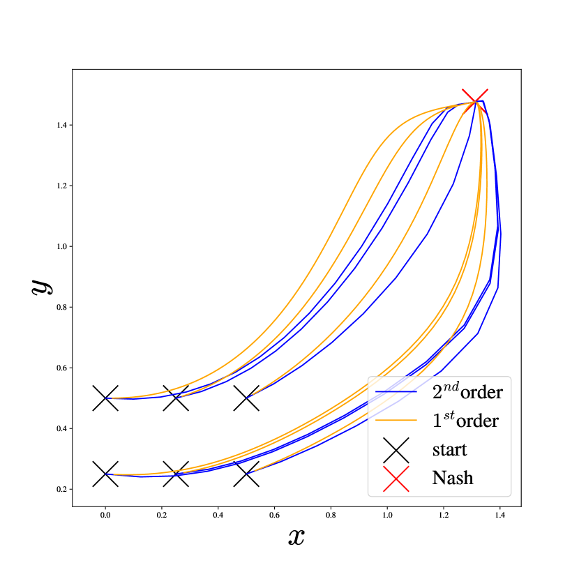
(a) The iterates of the algorithm

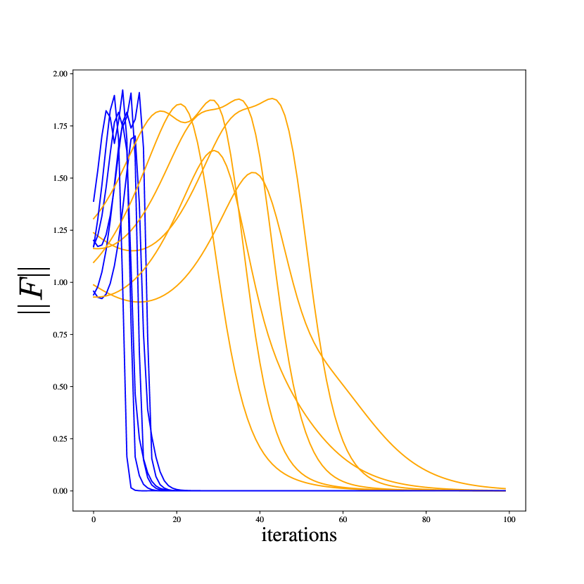
(b) The operator norm $\|F\|;$

Figure 1: 1st and 2nd Order method for the weak-MVI example (Modified-Forsaken). For the 1st order method we use $L_{1}=20$ and for the 2nd order method $L_{2}=50000$.

4.2 With the competitive operator $F_{\alpha}$

In this section we discuss simple extensions to our method that can be used to solve a larger class of saddle point problems.

While Diakonikolas et al. (2021) consider the weak-MVI condition for $F=\begin{bmatrix}\nabla_{x}f\\ -\nabla_{y}f\end{bmatrix}$ our results are for any general field $F$. Making use of this versatility we show that our method can be extended to include the parameterized competitive field $g_{\alpha}$ introduced in Vyas and Azizzadenesheli (2022). This field is important as following it allows us to obtain small operator norm for a different generalisation of the MVI condition, $\alpha$-MVI Vyas and Azizzadenesheli (2022). For the said field,

$$F_{\alpha}=\begin{bmatrix}I&\alpha\nabla_{xy}f\\ -\alpha\nabla_{yx}f&I\end{bmatrix}^{-1}\begin{bmatrix}\nabla_{x}f\\ -\nabla_{y}f\end{bmatrix}$$

the weak-MVI assumption (a₁) for $p=1$ contains the $\alpha$-MVI class. Note that if a field $F$ satisfies the $\alpha$-MVI condition, the corresponding field $F_{\alpha}$ satisfies the MVI condition.

We further note that the exact stationary points of $F_{\alpha}$ are the same as that of $F$. Thus an additional requirement of at least one SVI solution with $F_{\alpha}$ as the operator is satisfied if a solution to SVI with $F$ as the operator exists.

Using $F_{\alpha}$ as the field in question, we illustrate the first-order (which coincides with oCGO) and second order version of our algorithm on some examples satisfying the $\alpha$-MVI condition and show that our method performs faster than oCGO. Note that the first-order method is somewhere between first and second order while the second-order method is between second and third-order order in terms of the order of information of the gradient oracles. The second-order method can thus be thought of as a higher order oCGO.

Example 4.2.

We first consider the problem

$$\min_{x\in\mathcal{X}}\max_{y\in\mathcal{Y}}x^{2}y$$

Note that while all points on the $y$-axis are stationary points of the saddle point problem generated by $f(x,y)=x^{2}y$, there is only one global Nash equilibrium at the origin. However, when hoeg+uses $F$ as the operator the iterates converge to different points on $x=0$ as can be seen in Figure 2(a). Using $F_{\alpha}$ as the operator mitigates this issue of convergence to non Nash stationary points and as $\alpha$ increases, iterates from all the different initialization converge to the origin which is the Nash equilibrium, Figure 2(b). Theoretically mapping out the relation between the nature of stationary points and the operator used in our method, remains an open direction of research.

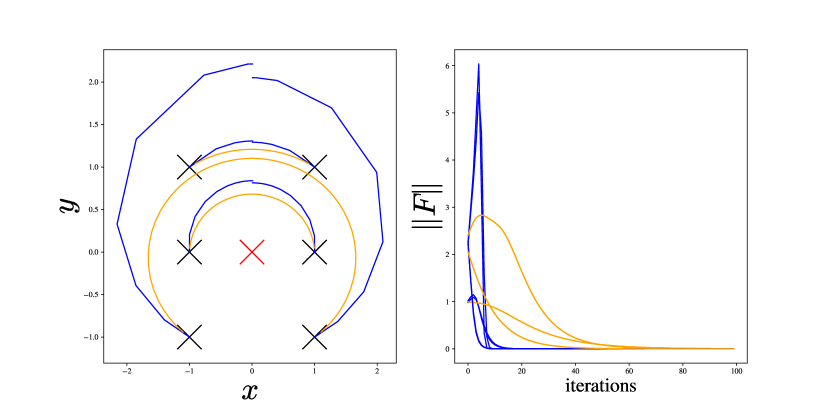
(a) $F$

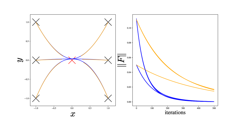
(b) $F_{\alpha};$ $\alpha=10$

Figure 2: 1st and 2nd Order method with $F_{\alpha}$ and $F$. For the 1st order method we use $L_{1}=20$ and for the 2nd order method $L_{2}=500$ as the Lipschitz constants for the operator

Example 4.3.

$$\min_{|x|\leq\frac{3}{2}}\max_{|y|\leq\frac{3}{2}}f(x,y)=x(y-0.45)+h(x)-h(y)$$ (Forsaken)

where $h(t)=\frac{t^{2}}{4}-\frac{t^{4}}{2}+\frac{t^{6}}{6}$.

We empirically study the Forsaken example in Pethick et al. (2022) and show that while using the gradient field $F=(\nabla_{x}f,-\nabla_{y}f)$ results in oscillation of both the 1st and 2nd order methods as can be seen in Figure 3, using $F_{\alpha}$ allows us to converge to the only stationary point of the function, $z^{*}=(0.0780,0.4119)$. This happens since even though the stationary point $z^{*}$ does not satisfy the $weak$-MVI condition for $F$, it satisfies (as we numerically verify) the weak-MVI (and MVI) condition for $F_{\alpha}$ , $\alpha\geq 2$.

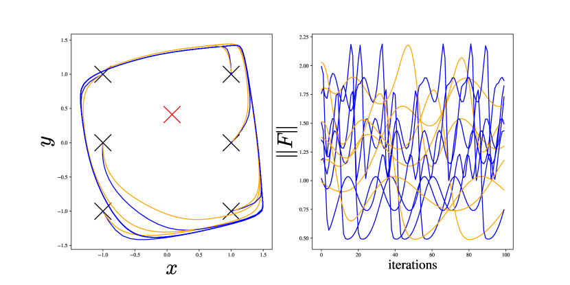
(a) $F$

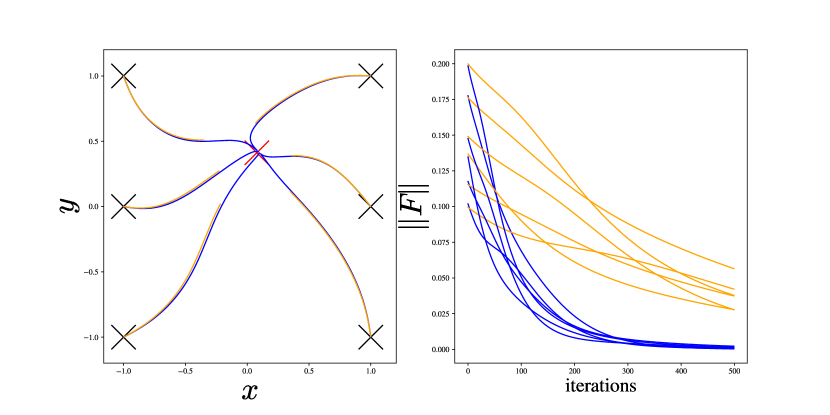
(b) $F_{\alpha};$ $\alpha=10$

Figure 3: First and second-order method with $F$ and $F_{\alpha}$ on (Forsaken). While the algorithm using $F$ cycles, using $F_{\alpha}$ the algrithm converges to a stationary point.

5 Conclusion

We propose higher-order methods for min-max problems satisfying a certain weak-MVI condition (Diakonikolas et al., 2021), whereby the $p^{th}$-order instance of our algorithm finds approximate stationary points at a rate of $O(\frac{1}{\epsilon^{\frac{p}{2}}})$. We further establish that, in the continuous-time limit, hoeg+gives rise to the dynamical system 3.1 (Lin and Jordan, 2022a), and the system obtains an analogous convergence rate as in the discrete-time setting. Finally we illustrate the performance of our algorithm experimentally for $p=1$ and $p=2$ using both the standard min-max operator $F=(\nabla_{x}f,-\nabla_{y}f)$ and the operator introduced by Vyas and Azizzadenesheli (2022), $F_{\alpha}$, demonstrating the potential advantage of our algorithm compared to first-order methods.

Appendix A Supporting Lemmas

We now present the supportive lemmas used to prove Lemma 3.3.

Let $\omega(z_{a},z_{b})$ denote the Bregman divergence of $h$, i.e.,

$$\omega(z_{a},z_{b})=h(z_{a})-h(z_{b})-\langle\nabla h(z_{b}),z_{a}-z_{b}\rangle$$

Lemma A.1 (Three Point Property).

Let $\omega(z,z_{b})$ denote the Bregman divergence of a function $h$. The three point property states, for any $z_{a},z_{b},z_{c}\in\mathcal{Z}$,

$$\langle\nabla h(z_{b})-\nabla h(z_{c}),z_{a}-z_{c}\rangle=\omega(z_{a},z_{c})+\omega(z_{c},z_{b})-\omega(z_{a},z_{b}).$$

Lemma A.2 (Tseng [2008]).

Let $\phi$ be a convex function, let $z_{a}\in\mathcal{Z}$, and let

$$z_{c}=\arg\min_{z^{\prime}\in\mathcal{Z}}\{\phi(z^{\prime})+\omega(z^{\prime},z_{a})\}.$$

Then, for all $z_{b}\in\mathcal{Z}$, we have, $\phi(z_{b})+\omega(z_{b},z_{a})\geq\phi(z_{c})+\omega(z_{c},z_{a})+\omega(z_{b},z_{c}).$

Finally, for the sake of completion, we provide here the proof of the key lemma from Adil et al. [2022] (Lemma 3.3).

A.1 Proof of Lemma 3.3

Proof.

For any $k$ and any $z\in\mathcal{Z}$, we first apply Lemma A.2 with $\phi(z)=\lambda_{k}\frac{p!}{L_{p}}\langle F(z_{k+\frac{1}{2}}),z-z_{k}\rangle$, which gives us

$$\lambda_{k}\frac{p!}{L_{p}}\langle F(z_{k+\frac{1}{2}}),z_{k+1}-z\rangle\leq\omega(z,z_{k})-\omega(z,z_{k+1})-\omega(z_{k+1},z_{k}).$$ (A.1)

Additionally, the guarantee of assumption a₂ with $z=z_{k+1}$ yields

$$\left\langle\tau_{p-1}(z_{k+\frac{1}{2}};z_{k}),z_{k+\frac{1}{2}}-z_{k+1}\right\rangle\leq\frac{2L_{p}}{p!}\omega(z_{k+\frac{1}{2}},z_{k})^{\frac{p-1}{2}}\left\langle\nabla h(z_{k})-\nabla h(z_{k+\frac{1}{2}}),z_{k+\frac{1}{2}}-z_{k+1}\right\rangle.$$ (A.2)

Applying the Bregmann three point property (Lemma A.1) and the definition of $\lambda_{k}$ to Equation A.2, we have

$$\lambda_{k}\frac{p!}{L_{p}}\left\langle\tau_{p-1}(z_{k+\frac{1}{2}};z_{k}),z_{k+\frac{1}{2}}-z_{k+1}\right\rangle\leq\omega(z_{k+1},z_{k})-\omega(z_{k+1},z_{k+\frac{1}{2}})-\omega(z_{k+\frac{1}{2}},z_{k}).$$ (A.3)

Summing Eqs. (A.1) and (A.3), we obtain

$$\lambda_{k}\frac{p!}{L_{p}}\left(\langle F(z_{k+\frac{1}{2}}),z_{i+\frac{1}{2}}-z\rangle+\left\langle\tau_{p-1}(z_{k+\frac{1}{2}};z_{k})-F(z_{i+\frac{1}{2}}),z_{k+\frac{1}{2}}-z_{k+1}\right\rangle\right)$$

$$\leq\omega(z,z_{k})-\omega(z,z_{k+1})-\omega(z_{k+1},z_{k+\frac{1}{2}})-\omega(z_{k+\frac{1}{2}},z_{k}).$$ (A.4)

Now, we obtain

$$\lambda_{k} \frac{p!}{L_{p}}\left\langle\tau_{p-1}(z_{k+\frac{1}{2}};z_{k})-F(z_{i+\frac{1}{2}}),z_{k+\frac{1}{2}}-z_{k+1}\right\rangle$$

$$\begin{subarray}{c}(i)\\ \geq\end{subarray}-\lambda_{k}\frac{p!}{L_{p}}\left\lVert\tau_{p-1}(z_{k+\frac{1}{2}};z_{k})-F(z_{i+\frac{1}{2}})\right\rVert_{*}\left\lVert z_{k+\frac{1}{2}}-z_{k+1}\right\rVert$$

$$\begin{subarray}{c}(ii)\\ \geq\end{subarray}-\lambda_{k}\left\lVert z_{i+\frac{1}{2}}-z_{k}\right\rVert^{p}\left\lVert z_{k+\frac{1}{2}}-z_{k+1}\right\rVert$$

$$\begin{subarray}{c}(iii)\\ \geq\end{subarray}-\frac{1}{2}\omega(z_{i+\frac{1}{2}},z_{k})^{-\frac{p-1}{2}}\omega(z_{i+\frac{1}{2}},z_{k})^{\frac{p}{2}}\omega(z_{k+1},z_{k+\frac{1}{2}})^{\frac{1}{2}}$$

$$=-\frac{1}{2}\omega(z_{i+\frac{1}{2}},z_{k})^{\frac{1}{2}}\omega(z_{k+1},z_{k+\frac{1}{2}})^{\frac{1}{2}}$$

$$\begin{subarray}{c}(iv)\\ \geq\end{subarray}-\frac{1}{16}\omega(z_{i+\frac{1}{2}},z_{k})-\omega(z_{k+1},z_{k+\frac{1}{2}})$$

Here, $(i)$ used Holder’s inequality, $(ii)$ used assumption a₂, $(iii)$ used the $1$-strong convexity of $\omega$, and $(iv)$ used the inequality $\sqrt{xy}\leq 2x+\frac{1}{8}y$ for $x,y\geq 0$. Combining with Eq. (A.1) and rearranging yields

$$\lambda_{k}\frac{p!}{L_{p}}\langle F(z_{k+\frac{1}{2}}),z_{i+\frac{1}{2}}-z\rangle\leq\omega(z,z_{k})-\omega(z,z_{k+1})-\frac{15}{16}\omega(z_{k+\frac{1}{2}},z_{k}).$$

We observe that by the choice of $\lambda_{k}$ in Algorithm 1, $\omega(z_{i+\frac{1}{2}},z_{k})=\left(2\lambda_{k}\right)^{-\frac{2}{p-1}}$. Applying this fact and summing over all iterations $i$ yields

$$\sum_{i=0}^{K}\lambda_{k}\frac{p!}{L_{p}}\langle F(z_{k+\frac{1}{2}}),z_{i+\frac{1}{2}}-z\rangle\leq\omega(z,z_{0})-\frac{15}{16}\sum_{i=0}^{K}\left(2\lambda_{k}\right)^{-\frac{2}{p-1}}$$

Finally substituting $z=z^{*}$ and setting the potential function $h(x)=\|x\|^{2}$ in $\omega$ gives us the statement of the lemma. ∎

Appendix B Results for de-coupled weak-MVI condition and $F_{\alpha}$

In this section we discuss the rates obtained when higher order methods are applied to the function which satisfy the original weak-MVI condition

Assumption 3 ($q^{th}$ Weak mvi).

There exists $z^{*}\in\mathcal{Z}^{*}$ such that:

$$(\forall z\in\mathbb{R}^{d}):\quad\left\langle F(z),z-z^{*}\right\rangle\geq-\frac{\rho}{2}\|F(z)\|^{q},$$ (a₃)

for some parameter $\rho$.

Theorem B.1.

For $F$ satisfying assumption (a₃) with $\rho\leq\frac{15}{16D^{q}}\frac{p!D}{L_{p}}^{\frac{p+1}{p}}$ and $D=\max_{k}L_{1}\|z_{k}-z^{*}\|$, running a $p^{th}$-order instance of our Algorithm (1) we have,

• for all $k\geq 1:$

  $$\frac{1}{k+1}\sum_{i=0}^{k}\|F(z_{k+\frac{1}{2}})\|^{\frac{2}{p}}\leq\frac{c\|z_{0}-z^{*}\|^{2}}{k+1}.$$

  In particular, we have that

  $$\min_{0\leq i\leq k}\|F(z_{k+\frac{1}{2}})\|^{\frac{2}{p}}\leq\frac{c\|z_{0}-z^{*}\|^{2}}{k+1}\rightarrow\min_{0\leq i\leq k}\|F(z_{k})\|^{2}\leq\frac{c_{1}}{(k+1)^{p}}$$

  and

  $$\mathbb{E}_{i\sim\mathrm{Unif}\{0,\dots,k\}}\big{[}\|F(z_{k})\|^{2}\big{]}\leq\frac{c\|z_{0}-z^{*}\|^{2}}{k+1}^{p}\leq\frac{C}{(k+1)^{p}},$$

  where $i\sim\mathrm{Unif}\{0,\dots,k\}$ denotes an index $i$ chosen uniformly at random from the set $\{0,\dots,k\}.$

• for $K=O(\frac{1}{\epsilon^{\frac{p}{2}}})$ number of iterations the output $z_{out}$ of Algorithm 1 is an $\epsilon$-approximate stationary point i.e., it satisfies $\|F(z_{out})\|\leq\epsilon$

Proof.

From Lemma 3.2 [Adil et al., 2022], for Algorithm (1), we have:

$$\sum_{i=0}^{K}\lambda_{k}\frac{p!}{L_{p}}\langle F(z_{k+\frac{1}{2}}),z_{k+\frac{1}{2}}-z^{*}\rangle\leq\|z_{0}-z^{*}\|^{2}-\frac{15}{16}\sum_{i=0}^{K}\|z_{k}-z_{k+\frac{1}{2}}\|^{2}$$ (B.1)

Adding $\sum_{k=1}^{K}\rho\lambda_{k}\|F(z_{k})\|^{q}$ to both sides of Eq. (B.1), and noting from Eq. (3.4) that,

$$\rho\lambda_{k}\|F(z_{k+\frac{1}{2}})\|^{q}=\|F(z_{k+\frac{1}{2}})\|^{(q-\frac{p+1}{p})}\rho\frac{\|F(z_{k+\frac{1}{2}})\|^{\frac{p+1}{p}}}{2\|z_{k}-z_{k+\frac{1}{2}}\|^{p-1}}\leq\rho(\frac{L_{p}}{p!})^{\frac{p+1}{p}}\|z_{k}-z_{k+\frac{1}{2}}\|^{2}\|F(z_{k+\frac{1}{2}})\|^{(q-\frac{p+1}{p})}$$

Further substituting $p=1$ in and choosing $x,y$ appropriately from (a₂) we obtain:

$$\|F(z_{k+\frac{1}{2}})\|\leq L_{1}\|z_{k+\frac{1}{2}}-z^{*}\|$$

further letting $D=\max_{k}L_{1}\|z_{k+\frac{1}{2}}-z^{*}\|$ we have,

$$\rho(\frac{L_{p}}{p!})^{\frac{p+1}{p}}\|z_{k}-z_{k+\frac{1}{2}}\|^{2}\|F(z_{k+\frac{1}{2}})\|^{(q-\frac{p+1}{p})}\leq\rho D^{q}(\frac{L_{p}}{p!D})^{\frac{p+1}{p}}\|z_{k}-z_{k+\frac{1}{2}}\|^{2}$$

.

Thus,

$$\sum_{i=0}^{K}\lambda_{k}(\frac{p!}{L_{p}}\langle F(z_{k+\frac{1}{2}}),z_{k+\frac{1}{2}}-z^{*}\rangle+\rho\|F(z_{k+\frac{1}{2}})\|^{q})\leq \|z^{*}-z_{0}\|^{2}$$ (B.2)

$$- (\frac{15}{16}-\rho D^{q}(\frac{L_{p}}{p!D})^{\frac{p+1}{p}})\sum_{i=0}^{K}\|z_{k}-z_{k+\frac{1}{2}}\|^{2}$$

From assumption (a₃) we have that LHS in Eq. (B.2) is non-negative. Setting $c_{2}=(\frac{15}{16}-\rho D^{q}(\frac{L_{p}}{p!D})^{\frac{p+1}{p}})$ and using Lemma 3.4 we get,

$$c_{2}\sum_{i=0}^{K}\|F(z_{k+\frac{1}{2}})\|^{\frac{2}{p}}\leq c_{2}\sum_{i=0}^{K}\|z_{k}-z_{k+\frac{1}{2}}\|^{2}\leq\|z^{*}-z_{0}\|^{2}$$

And thus we obtain results analogous to Theorem 3.5. Furthermore, setting $q=2$ gives us rates for the $p^{th}$-order versions of hoeg+for the weak-MVI condition in [Diakonikolas et al., 2021] ∎

We now present the result on the convergence of $F_{\alpha}$ when used as the operator in our algorithm. As a corollary of Theorem 3.5 we have,

Corollary B.2.

Let the competitive field $F_{\alpha}$ satisfy the smoothness and weak-MVI assumptions (a₁), (a₂) then for algorithm (1) using $F_{\alpha}$ we have,

• for all $k\geq 1:$

  $$\frac{1}{K+1}\sum_{k=0}^{K}\|F_{\alpha}(z_{k+\frac{1}{2}})\|^{\frac{2}{p}}\leq\frac{\|z_{0}-z^{*}\|^{2}}{c_{2}(K+1)}.$$

  In particular, we have that

  $$\min_{0\leq k\leq K}\|F_{\alpha}(z_{k+\frac{1}{2}})\|^{\frac{2}{p}}\leq\frac{\|z_{0}-z^{*}\|^{2}}{c_{2}(K+1)}\rightarrow\min_{0\leq k\leq K}\|F_{\alpha}(z_{k+\frac{1}{2}})\|^{2}\leq\frac{C}{(K+1)^{p}}$$

  where $C=\frac{\|z_{0}-z^{*}\|^{2p}}{c_{2}^{p}}$ and

  $$\mathbb{E}_{k\sim\mathrm{Unif}\{0,\dots,K\}}\big{[}\|F_{\alpha}(z_{k+\frac{1}{2}})\|^{2}\big{]}\leq(\frac{\|z_{0}-z^{*}\|^{2}}{c_{2}(K+1)})^{p}\leq\frac{C}{(K+1)^{p}},$$

  where $k\sim\mathrm{Unif}\{0,\dots,K\}$ denotes an index $i$ chosen uniformly at random from the set $\{0,\dots,K\}.$

• for $K=O(\frac{1}{\epsilon^{\frac{p}{2}}})$ number of iterations the output $z_{out}$ of Algorithm 1 is an $\epsilon$-approximate stationary point i.e., it satisfies $\|F(z_{out})\|\leq\epsilon$

References

• Adil et al. (2022) D. Adil, B. Bullins, A. Jambulapati, and S. Sachdeva. Optimal methods for higher-order smooth monotone variational inequalities. arXiv preprint arXiv:2205.06167, 2022.
• Agarwal et al. (2017) N. Agarwal, Z. Allen-Zhu, B. Bullins, E. Hazan, and T. Ma. Finding approximate local minima faster than gradient descent. In Proceedings of the 49th Annual ACM SIGACT Symposium on Theory of Computing, pages 1195–1199, 2017.
• Ben-Tal et al. (2009) A. Ben-Tal, L. El Ghaoui, and A. Nemirovski. Robust optimization, volume 28. Princeton University Press, 2009.
• Birgin et al. (2017) E. G. Birgin, J. Gardenghi, J. M. Martínez, S. A. Santos, and P. L. Toint. Worst-case evaluation complexity for unconstrained nonlinear optimization using high-order regularized models. Mathematical Programming, 163:359–368, 2017.
• Bullins and Lai (2022) B. Bullins and K. A. Lai. Higher-order methods for convex-concave min-max optimization and monotone variational inequalities. SIAM Journal on Optimization, 32(3):2208–2229, 2022.
• Carmon et al. (2017) Y. Carmon, J. C. Duchi, O. Hinder, and A. Sidford. “convex until proven guilty”: Dimension-free acceleration of gradient descent on non-convex functions. In International conference on machine learning, pages 654–663. PMLR, 2017.
• Carmon et al. (2018) Y. Carmon, J. C. Duchi, O. Hinder, and A. Sidford. Accelerated methods for nonconvex optimization. SIAM Journal on Optimization, 28(2):1751–1772, 2018.
• Carmon et al. (2020) Y. Carmon, J. C. Duchi, O. Hinder, and A. Sidford. Lower bounds for finding stationary points i. Mathematical Programming, 184(1-2):71–120, 2020.
• Carmon et al. (2021) Y. Carmon, J. C. Duchi, O. Hinder, and A. Sidford. Lower bounds for finding stationary points ii: first-order methods. Mathematical Programming, 185(1-2):315–355, 2021.
• Daskalakis et al. (2021) C. Daskalakis, S. Skoulakis, and M. Zampetakis. The complexity of constrained min-max optimization. In Proceedings of the 53rd Annual ACM SIGACT Symposium on Theory of Computing, pages 1466–1478, 2021.
• Diakonikolas (2020) J. Diakonikolas. Halpern iteration for near-optimal and parameter-free monotone inclusion and strong solutions to variational inequalities. In Conference on Learning Theory, pages 1428–1451. PMLR, 2020.