Progressive Visual Prompt Learning with Contrastive Feature Re-formation

Abstract

Prompt learning has been designed as an alternative to fine-tuning for adapting Vision-language (V-L) models to the downstream tasks. Previous works mainly focus on text prompt while visual prompt works are limited for V-L models. The existing visual prompt methods endure either mediocre performance or unstable training process, indicating the difficulty of visual prompt learning. In this paper, we propose a new Progressive Visual Prompt (ProVP) structure to strengthen the interactions among prompts of different layers. More importantly, our ProVP could effectively propagate the image embeddings to deep layers and behave partially similar to an instance adaptive prompt method. To alleviate generalization deterioration, we further propose a new contrastive feature re-formation, which prevents the serious deviation of the prompted visual feature from the fixed CLIP visual feature distribution. Combining both, our method (ProVP-Ref) is evaluated on 11 image benchmark datasets and achieves 7/11 state-of-the-art results on both few-shot and base-to-novel settings. To the best of our knowledge, we are the first to demonstrate the superior performance of visual prompts in V-L models to previous prompt-based methods in downstream tasks. Meanwhile, it implies that our ProVP-Ref shows the best capability to adapt and to generalize.

1 Introduction

Vision-language (V-L) pre-trained models such as CLIP  [33] have showed great potential in many tasks [9, 49, 4, 20, 44, 10, 12, 7, 38]. Instead of using closed-set category labels, V-L models are pre-trained to align visual and text features with web-scale of text-image pairs. Supervised by rich natural language, the models are capable of learning open-set visual concepts and have strong generalization capability. However, how to transfer CLIP to downstream tasks effectively still remains an open question. Fine-tuning the entire model leads to high risk of overfitting and may catastrophically forget the useful pre-trained knowledge due to the numerous tunable parameters, especially when training data is scarce. Moreover, in fine-tuning paradigm, each task would have an unique large-scale model, resulting in a cost raise of storage and model deployment.

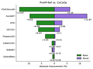
Figure 1: Absolute gains of ProVP-Ref over CoCoOp [50] in base-to-novel generalization on 8 datasets. ProVP-Ref shows a significant improvement on both base and novel classes.

To address the challenges above, prompt learning  [51, 50, 52] has been used for adapting V-L models to the downstream tasks with a small amount of learnable prompts, keeping the original pre-trained model frozen. Encouraged by the success of prompt learning in natural language processing [24, 19, 21], existing works mainly focus on text branch such as CoOp [51], CoCoOp [50], ProGrad [52]. However, prompting the image encoder is much less explored. It is expected that prompting in visual stream could enable the pre-trained V-L model to better handle the image data distribution shift and adapt to new domains effectively.

From the limited literature [1, 17], visual prompt is difficult to optimize in the current design. For instance, Bahng et al. [1] explored visual prompts with CLIP by padding learnable pixels but fail to achieve downstream performance improvement to full fine-tuning. Jia et al. [17] developed a deep visual prompt tuning (VPT) approach for single-modal Vision Transformer (ViT) [6] models. Their training phase is unstable and sensitive to hyper-parameters. In addition, its random initialized prompts inserted into each layer of ViT are learned independently. Such structure lacks the interaction between the prompts in different layers and causes large perturbations to the pre-trained model, resulting in a higher overfitting risk on small data.

Based on the above analysis, in this paper, we focus on visual prompt learning with V-L models by proposing a new Progressive Visual Prompt (ProVP) structure. Different from VPT [17], our ProVP connects the prompts from adjacent layers in a progressive manner: the input prompt embedding to the current layer is based on the combination of the new inserted prompts and the output of prompt embedding from the previous layer. Through this structure, the interaction between prompts of different layers is strengthened, which improves the effectiveness and efficiency of prompt learning and stabilizes the training process. More importantly, through this residual connection between adjacent prompts, our ProVP could effectively propagate the image embeddings to deep layers and behave partially in an instance adaptive manner. Similar to CoCoOp  [50], we found such structure can focus on learning instance-level information rather than the subsets of classes, which helps to prevent overfitting and be more robust to domain shifts.

Besides the novel ProVP structure, we further address the generalization deterioration problem of prompt learning, (e.g., after training, the model capability of recognizing unseen classes significantly drops). To alleviate this, in this paper, we propose a new contrastive feature re-formation method to incorporate constraint on the prompted visual feature. As random initialized prompts may cause a large shift on pre-trained features, we maintain the generalization capability of the model via reformating the prompted output features under the guidance of the visual feature distribution in CLIP. Different from [52], our method retains the pre-trained knowledge in the feature space, which is more flexible to hanle the downstream tasks with large domain gaps. The main contributions are summarized as follows:

• We investigate the visual prompts with CLIP and propose a novel progressive visual prompt (ProVP) structure. To the best of our knowledge, we are the first to demonstrate the effectiveness of visual prompts in V-L pre-trained models and show its superior performance over previous prompt-based methods in downstream tasks (Fig. Figure 1).

• To alleviate generalization deterioration, we further propose a new contrastive feature re-formation, which prevents the serious deviation of the prompted visual feature from CLIP visual feature distribution. With designed feature constraint, our model can improve adaptation and generalization capability simultaneously.

• We evaluate our method on 11 image benchmark datasets and achieve 7/11 state-of-the-art (SOTA) results on both few-shot and base-to-novel settings. Notably, our method provides significant gains over text prompt counterparts on the datasets that have larger distribution shifts.

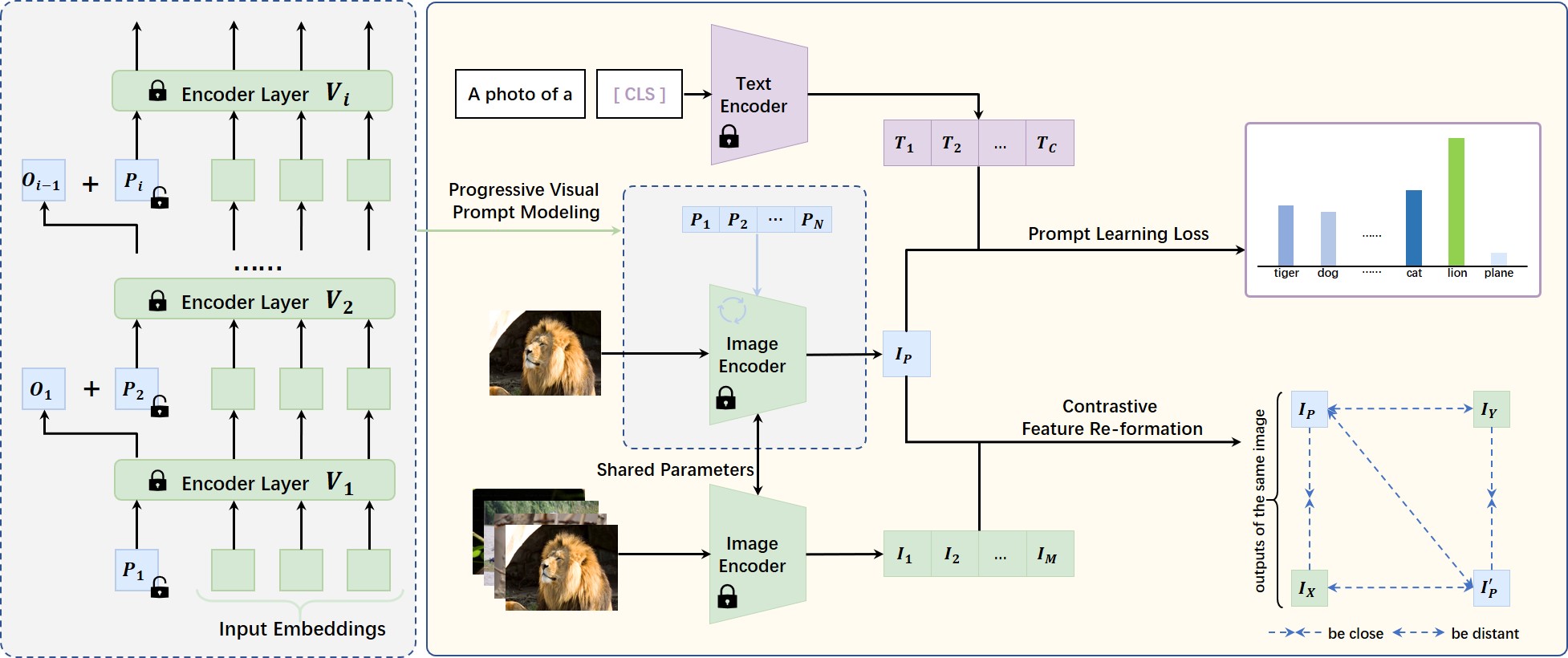
Figure 2: An overview of ProVP-Ref. Right: a full pipeline for our approach. It consists of two main parts as Progressive Visual Prompt, in which we retain the outputs of prompt via a progressive connection, and Contrastive Feature Re-formation: Using the frozen image encoder and the original image input, we can reformate the prompted features so that they can constitute a more similar representation with pre-trained CLIP. Left: a detailed view of Progressive Visual Prompt, new prompts will be combined with the output of the former embeddings before being sent to the encoder layer.

2 Related Work

Vision-Language Models

Large-scale vision-language (V-L) models, like CLIP [33], ALIGN [16], Florence [47], LiT [48], DeCLIP [22], become prevalent in computer vision community because of its robust representation and generalization capability. These models usually consist of a visual encoder (e.g., ViT [6]) and a text encoder (e.g., Transformer [42]), which are pre-trained to align visual and text encoded features via contrastive learning with large scale of text-image pairs (e.g., $\sim$400M for CLIP and $\sim$1B for ALIGN). They have showed great potential in many tasks, such as image classification [9, 49, 4], semantic segmentation [20, 44, 10], object detection [12, 7, 38] and image captioning [28, 41, 37]. In this work, we use CLIP as the foundation model of our method.

Prompt Learning in Vision-Language Models

Inspired by the popularity of prompt learning in NLP [24, 19, 21], pioneering work of prompt learning for V-L models mainly focus on text encoder [51, 50, 52, 26, 39], while keeping image encoder untouched. CoOp [51] firstly proposes learnable text prompt instead of the hand-crafted prompt (e.g., ’A photo of a’) to adapt CLIP model for few-shot classification. CoCoOp [50] identifies the generalization problem of CoOp and develops an extra Meta-Net to produce instance-level prompts conditioned on each image, which was evaluated on a base-to-novel setting to demonstrate its superior performance on unseen classes. ProGrad [52] only updates the prompt whose gradient is aligned to the hand-crafted prompt on zero-shot settings in order to prevent forgetting the pre-trained knowledge of CLIP. ProDA [26] extends CoOp by optimizing multiple text prompts simultaneously and estimates the distribution of the output embeddings of the prompts. TPT [39] proposes test-time prompt tuning that learns adaptive text prompts on the fly with a single test sample. Compared with text prompt learning, visual prompt learning in V-L models is much less explored. Bahng et al. [1] firstly explored visual prompts with CLIP in pixel space by padding learnable pixels around the input images. Such pixel-level prompt is difficult to learn and the tuned performance is unsatisfied compared to full fine-tuning. Recently, VPT [17] was proposed to insert visual prompts in embedding space into a ViT [6] in a shallow or deep manner where the prompts were inserted into each layer of ViT and learned independently. It was built on a single-modal model while the more powerful V-L models, such as CLIP, has not been attempted. Some other works [45, 43] also make use of visual prompts, but were invented specifically for incremental learning. Our work differs from these works as we focus on the visual prompt learning with V-L models while the text encoder is kept frozen. A novel progressive visual prompt structure is also proposed which is different from VPT and not investigated before.

Knowledge Transfer

Although forgetting mitigation has been widely explored in incremental learning [25, 15, 32, 34, 23, 36], such methods can not be employed for prompt learning directly. In incremental learning, it aims at continually learning new knowledge without forgetting the previous ones, avoiding the performance drop of previous tasks. In prompt learning, on the contrary, forgetting mitigation helps the model capture the relevant knowledge from the large-scale pre-trained knowledge of V-L models, which eventually benefits the performance on downstream tasks. Identifying such differences, Zhu et al. [52] use a gradient align method to learn prompts without conflicting with the pre-trained knowledge (e.g., zero-shot CLIP predictions). However, over-reservation of general knowledge in prompt learning may distract the training process, which causes an insufficient learning. We relieve this problem by constraining the learned prompts on the feature space via contrastive learning, which is more flexible for keeping useful information from pre-trained knowledge in V-L models.

3 Method

3.1 Revisit CLIP and VPT

CLIP

[33] is formed by a decoupled text and image encoder pair and pre-trained by language-image contrastive learning. Specifically, given a mini-batch text-image pairs, the model maximizes the similarity of the paired text-image encoded features while minimizes the unpaired ones. After training, CLIP can be utilized in zero-shot recognition tasks with a hand-crafted template prompt (e.g., ’a photo of a $<$category$>$’). Denote $\{l_{i}\}^{C}_{i=1}$ as the label set containing $C$ classes of a downstream task, the template prompted embeddings $\{t_{i}\}^{C}_{i=1}$ will be fed into the text encoder $g(\cdot)$. Let $<\cdot,\cdot>$ be cosine similarity, given the image encoder $f(\cdot)$ and a test image $x$, CLIP gives the prediction based on the maximum probability, which is defined as:

$$\centering p(t_{i}|x)=\frac{exp(<f(x),g(t_{i})>/\tau)}{\sum\limits_{j=1}^{C}exp(<f(x),g(t_{j})>/\tau)},\@add@centering$$ (1)

and $\tau$ is a temperature parameter learned by CLIP.

Visual Prompting Tuning

[17] inserts learnable token embeddings (visual prompts) into the input latent space of ViT [6], and tunes them while freezes model backbone. In VPT, Two types of visual prompting are designed: VPT-Shallow and VPT-Deep. And VPT-Deep is proved to perform better on transfer learning tasks. Formally, denoting a collection of $m$ learnable $d$-dimension prompts as $P_{i}=\{p_{i}^{k}\in\mathbb{R}^{d}|k=1,2,...,m\}$ for the $i_{th}$ layer $L_{i}$, VPT-Deep displays the prompt insertion in a ViT [6] with $N$ layers as:

$$[X_{i},\underline{\hbox to8.53581pt{}}]=L_{i}([X_{i-1},P_{i}]),\quad i=1,2,...,N.$$ (2)

And $X_{i}$ represents the original input embeddings for the $(i+1)_{th}$ layer. However, we found the training process of VPT-Deep is tough: the independent learning of prompts in each layer may confuse the direction of optimization, increasing the difficulty of training and making the model sensitive to hyper-parameters. Besides, the random initialized prompts at each layer in VPT is likely to cause large perturbations to the model output, which brings a high risk of catastrophic forgetting.

3.2 Progressive Visual Prompt Learning

In VPT-Deep, each prompt only participates in the propagation of its own layer: after the $i_{th}$ layer, the output for the prompt $P_{i}$, denoted as $O_{i}$, is discarded. These discarded prompt outputs could contain abundant information of the pre-trained models, which may benefit the eventual performance. To recall such discarded prompts we propose a new prompt learning structure as Progressive Visual Prompt (short for ProVP). ProVP utilizes a progressive connection to combine new inserted prompt embeddings and the former outputs. Formally, in ProVP, the prompting strategy of the visual encoder is modified as:

$$[X_{1},O_{1}]=L_{1}([X_{0},P_{1}]),$$ (3)

for the first layer $L_{1}$,and

$$\left[X_{i},O_{i}\right]=L_{i}([X_{i-1},(1-\alpha)*P_{i}+\alpha*O_{i-1}]),$$ (4)

for the following layers $i=2,...,N$, where $\alpha$ is the progressive decay for our ProVP. Prompt locations were v erified equivalent in VPT [17] paper as $[X_{i},O_{i}]$ or $[O_{i},X_{i}]$ and we follow original settings to insert visual prompts in the middle of image embeddings and the class token.

Compared with a deep-like structure, the progressive connections in ProVP act as an instance adaptive manner: the prompt output of the former block $O_{i}$ is deeply correlated to the image embeddings and varies with inputs while the new insert prompt $P_{i}$ is still input invariant. Thus, $P^{\prime}_{i}=(1-\alpha)P_{i}+\alpha*O_{i}$ also changes from different images. Similar to CoCoOp [50], we found such architecture pays more attention on the instance-level information rather than focusing on the subset of classes, which helps to prevent overfitting and be more robust to domain shifts. Also, the interaction between adjacent prompts is strengthened in the model, as a result, the oscillation of performance and sensitivity to hyper-parameters are alleviated (see the supplemental materials for the details), leading to a much more stable training. (e.g., we use the same prompt length for all datasets and almost the same hyper-parameters.)

During ProVP tuning, the text encoder is kept frozen. We use the hand-crafted template combined with labels as the input to the text encoder. Let $f_{\mathbf{p}}$ be the prompt tuned image encoder, we optimize the model by minimizing the negative log-likelihood:

$$\centering\begin{split}Loss_{ce}(x)&=-\sum\limits^{C}_{i=1}y_{i}\log p(t_{i}|x),\\ p(t_{i}|x)&=\frac{exp(<f_{\mathbf{p}}(x),g(t_{i})>/\tau)}{\sum\limits_{j=1}^{C}exp(<f_{\mathbf{p}}(x),g(t_{j})>/\tau)},\end{split}\@add@centering$$ (5)

where $y$ denotes the one-hot ground-truth annotation.

3.3 Contrastive Feature Re-formation

An overview of our approach is shown in Figure 2. When adapting pre-trained models to downstream tasks by prompt learning, generalization deterioration easily occurs. (e.g., the performance of CoOp [51] drops significantly when testing on unseen classes after training). One possible reason found by [52] is the improper learning for prompts. Using the cross entropy loss Eq. (5) alone may make the model forget the pre-trained general knowledge and focus on some specific downstream data suboptimally. To this end, Zhu et al.  [52] use the predicted logits of zero-shot CLIP to regularize the gradient direction when optimizing the prompts. However, the overemphasis on zero-shot CLIP predictions may lead to an insufficient learning of downstream knowledge and therefore an inferior performance. Motivated by [52] and knowledge distillation [14, 31], we specifically design a new training strategy, as Contrastive Feature Re-formation, for visual prompt learning. Instead of preserving the zero-shot CLIP predictions, we maintain the model generalizability under the guidance of the pre-trained image feature distribution.

As the random initialized prompts cause a large shift on the pre-trained features, the diversity of the prompted features may be reduced after training. To overcome this, we propose $Loss_{Ref}$ to reformate the shifted features so that they could constitute a similar distribution as the pre-trained CLIP: let $f$, $f_{\mathbf{p}}$ be the pre-trained and prompted image encoder, and $\{x_{i}\}^{M}_{i=1}$ represents a mini-batch of $M$ images. We constrain the tuned and pre-trained features of the same image $x_{i}$ to be close while the different ones to be distant. Therefore, the reformating loss is defined as

$$Loss_{Ref}(x_{i})=-\log\frac{exp(<f_{\mathbf{p}}(x_{i}),f(x_{i})>)}{\sum\limits_{j=1}^{M}exp(<f_{\mathbf{p}}(x_{i}),f(x_{j})>)}.$$ (6)

Combining with the $Loss_{ce}$ in Eq. (5), the total training loss can be formulated as :

$$\centering Loss=Loss_{ce}+\lambda Loss_{Ref},\@add@centering$$ (7)

where $\lambda\in[0,1]$ is a hyper-parameter to adjust the weight of the $Loss_{Ref}$ during training.

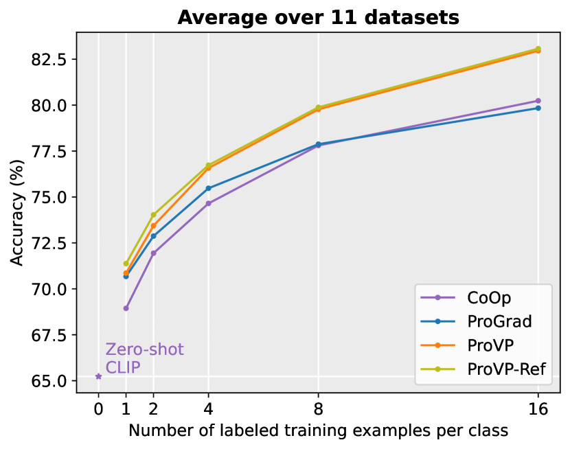
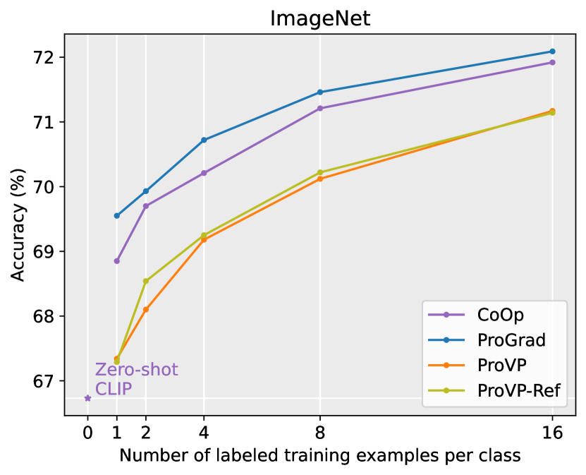
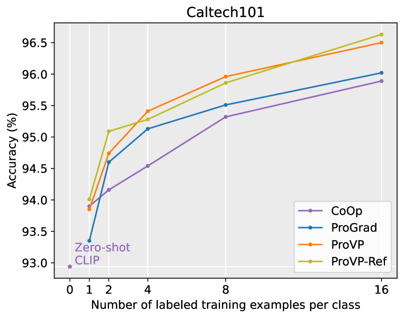
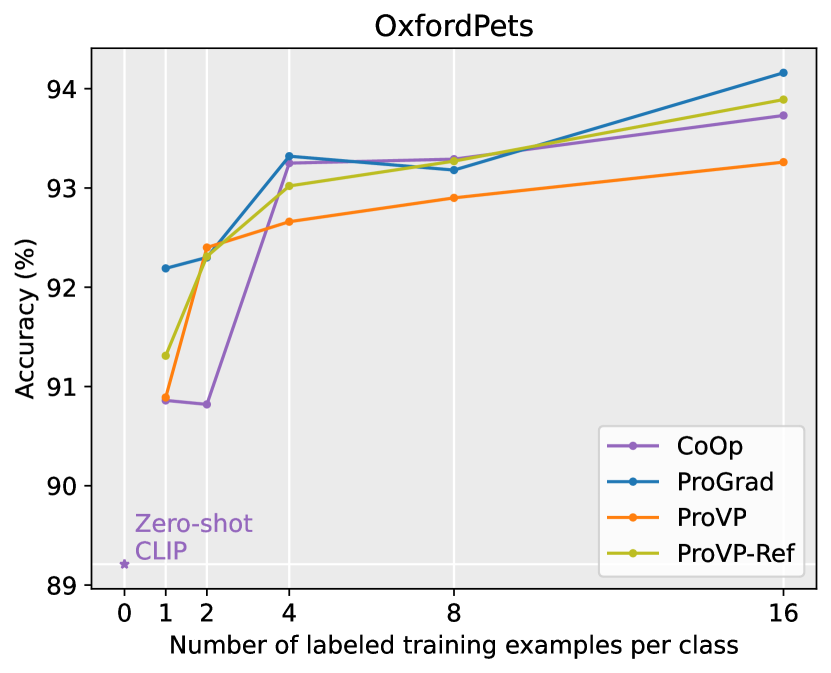
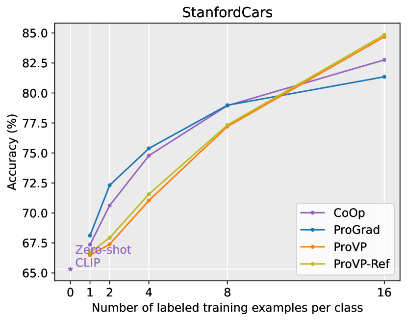
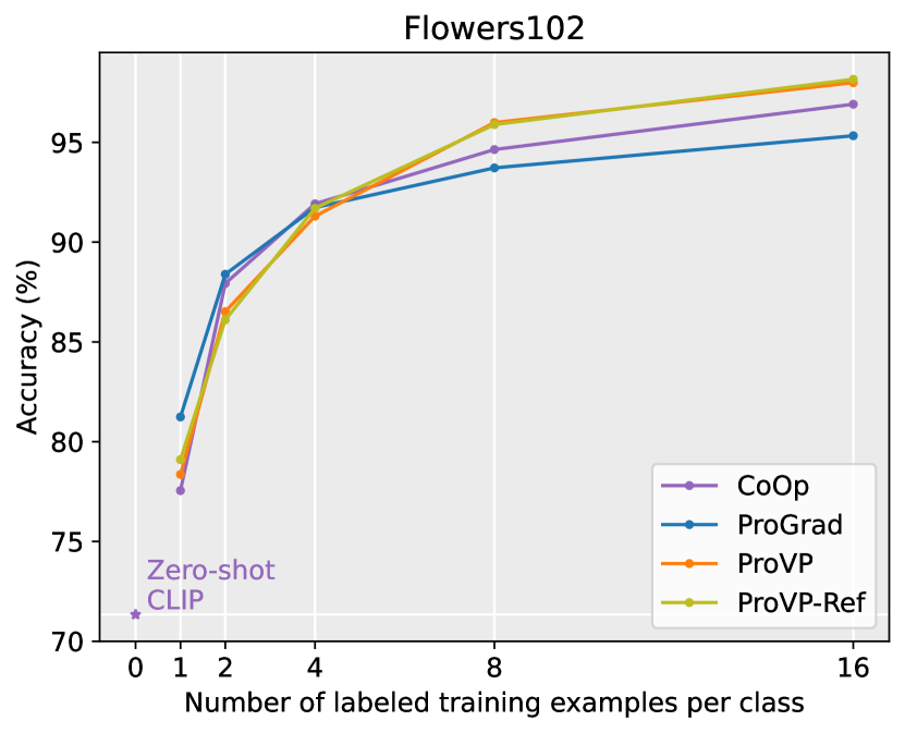
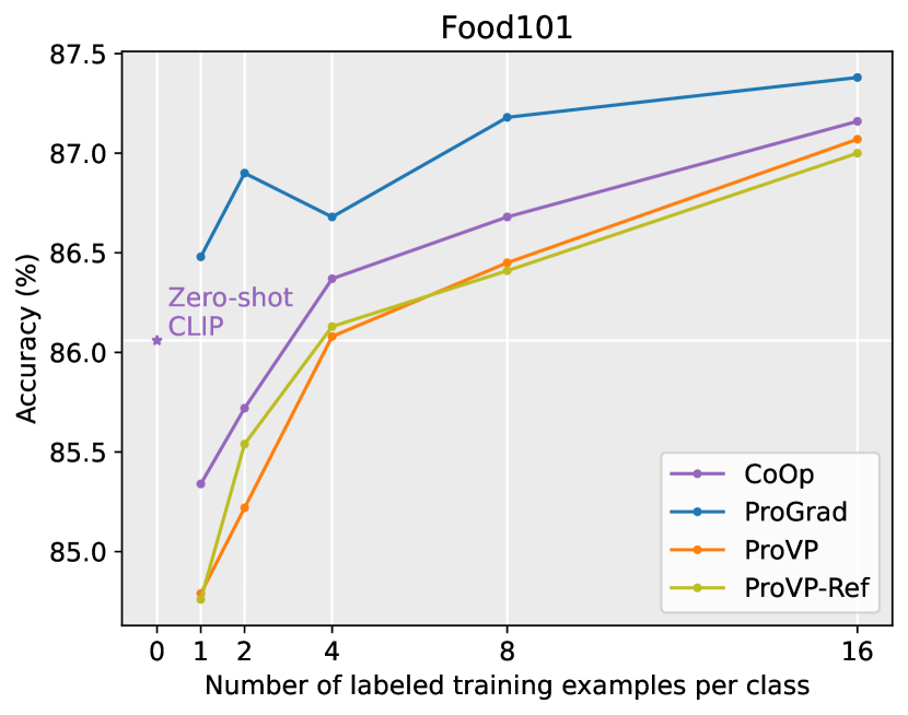
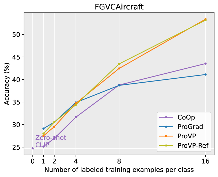
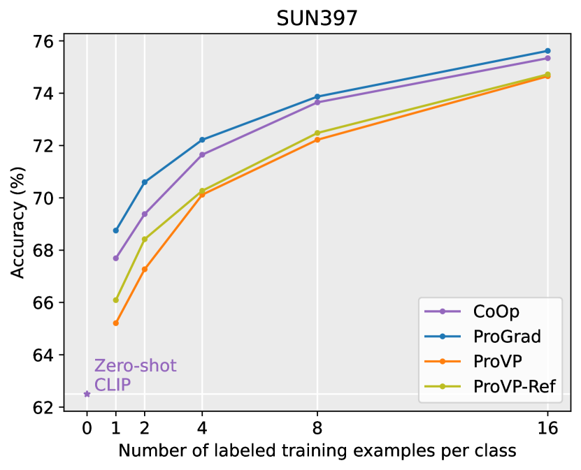
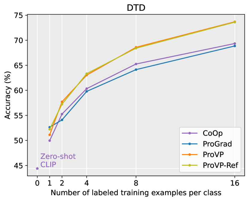
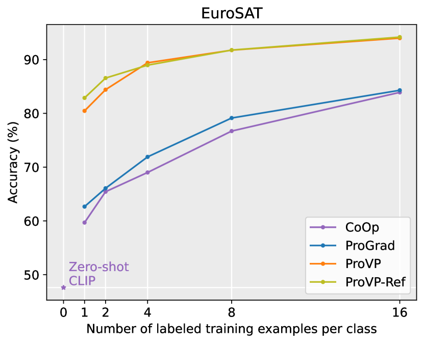
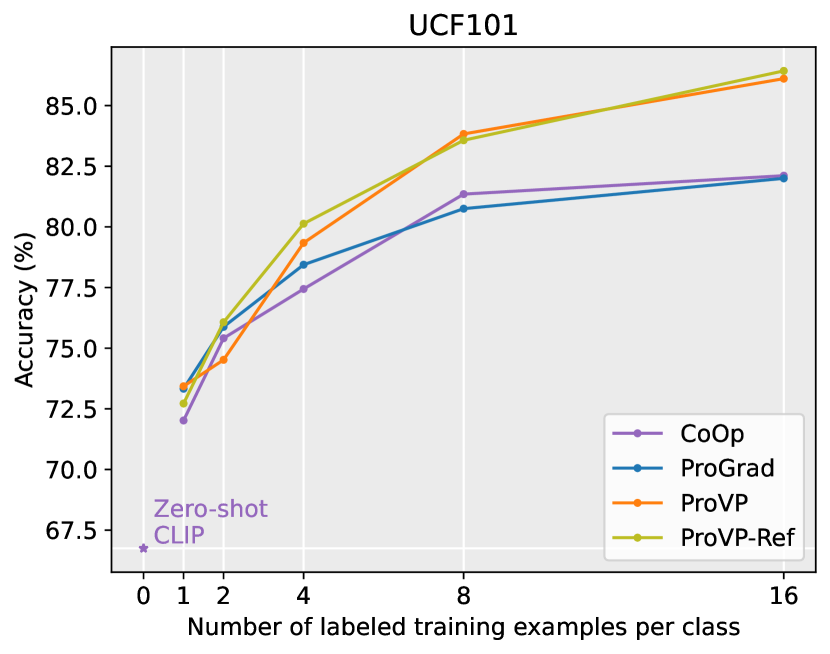
Figure 3: Full comparison of ProVP-Ref with previous methods on few-shot learning. ProVP-Ref shows significant gains in 7/11 datasets and highly improves the average performance.

Benefited from the such strategy, our model as ProVP-Ref can learn a more generalizable representation from pre-trained feature distribution. Moreover, by relieving the logits restriction in [52], our model would be less affected by the conflict pre-trained knowledge and still adaptable in the downstream task where exists large domain shifts.

4 Experiments

We evaluate the adaptation and generalization capability of our model in two settings: few-shot learning (B.1) and generalization from base-to-novel classes (B.2).

Datasets

Following CoOp [51] and CoCoOp [50], we use 11 image benchmark datasets in both settings: ImageNet [5], Caltech101 [8], FGVCAircraft [27], Flowers102 [29], Food101 [2], OxfordPets [30], StanfordCars [18], EuroSAT [13], DTD [3], SUN397 [46] and UCF101 [40].

For few-shot learning, following prior works [33, 51, 52], we train the model with 1, 2, 4, 8 and 16 shots and test on full test sets. For base-to-novel generalization, we train the model on a 16-shot setting for a fair comparison. The results are represented as the average over three runs.

Training Details

Our implementation is based on the open-source CLIP [33] with ViT-B/16 [6]. We use Xavier[11] for prompt initialization as VPT [17]. Progressive decay $\alpha$ is fixed as $0.1$. All models are trained with a batch size of 32 and a learning rate of 0.1 with SGD optimizer while we found the datasets with numerous categories (ImageNet [5] and SUN397 [46]) would benefit from a large learning rate of 5.0. All experiments are implemented on one single NVIDIA A100 GPU.

For few-shot learning, visual prompt length at each layer is set to 50. The maximum epoch is set to 200 for 16/8 shots, 100 for 4/2 shots, and 50 for 1 shot for all datasets. $\lambda$ is set as 0.1 for ImageNet, StanfordCars and OxfordFlowers and 1 for remaining datasets. For base-to-novel generalization, we shorten the prompt length to 16 and the maximum epoch to 100. $\lambda$ is set to 1 except ImageNet for 0.1.

4.1 Few-Shot Learning

Few-shot learning is a scenario that models are trained with a few labelled samples per class. The full results are shown in Figure 3. Comparing the average performance over 11 datasets, ProVP-Ref shows a significant improvement over all previous works in all shot settings. Particularly, ProVP-Ref gains an absolute improvement as $\mathbf{2.83}$% compared to the previous SOTA (CoOp) on 16 shots, which demonstrates the strong adaptation capability of our method. Also, contrastive feature re-formation improves the performance under small shots (e.g., 1-shot).

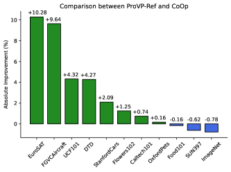
Figure 4: Comparison between ProVP-Ref and CoOp [51] in few-shot learning (16-shot setting).

The detailed comparison between our ProVP-Ref and CoOp is displayed in Figure 4. ProVP-Ref makes an obvious improvement over datasets which has large domain shifts from the pre-trained data, such as EuroSAT (+10.28%), FGVCAircraft (+9.64%), UCF101 (+4.32%) and DTD (+4.27%) and also gains improvement on fine-grained datasets such as StanfordCars (+2.09%) and Flowers102 (+1.25%). For ImageNet and SUN397, we found the less appealing results are mainly caused by the intrinsic drawback of CLIP [33]:for zero-shot recognition, the text features of CLIP have low distinguishability between different classes, and the distinguishability gets worse when the number of classes increases [35] (e.g., 1000 for ImageNet and 397 for SUN397). As we froze the text branch and leveraged such text features directly, the ambiguous text features may confuse the training of visual prompts, leading to a sub-optimal result.

To overcome such problem, we tried to extend our method by replacing the hand-crafted prompts by the learned text embeddings (e.g., learned prompts in CoOp) and keeping them frozen during the visual prompt learning. This extension, denoted as ProVP-Ref^∗, improves the performance on ImageNet (+1.49%) and SUN397 (+1.46%). Supported by the results shown in Table 1, ProVP-Ref^∗ has proved the effectiveness of our method in the remained tasks and reaches the top over all datasets.

Table 1: Results of ProVP-Ref^∗. Average_All indicates the average performance over all datasets.

	ImageNet	SUN397	Average_All
CoOp	71.92	75.34	80.24
ProGrad	72.09	75.62	79.84
ProVP-Ref	71.14	74.72	83.07
ProVP-Ref∗	72.63	76.18	83.41

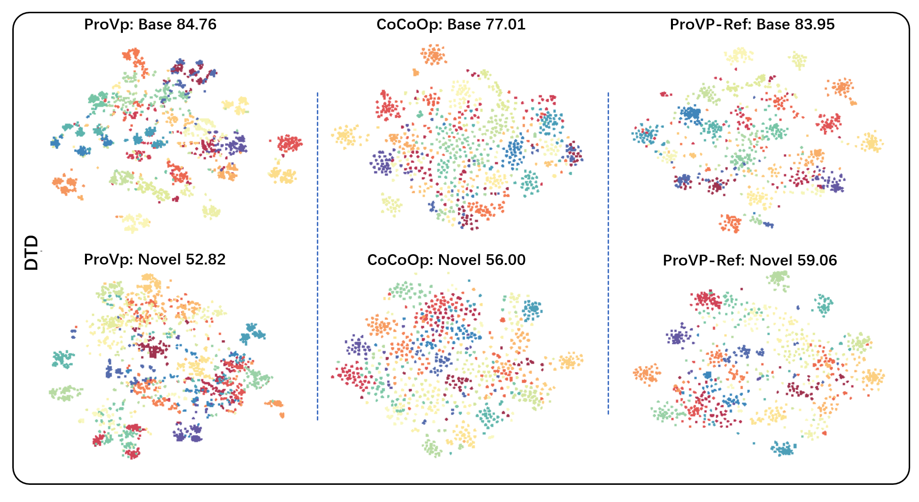
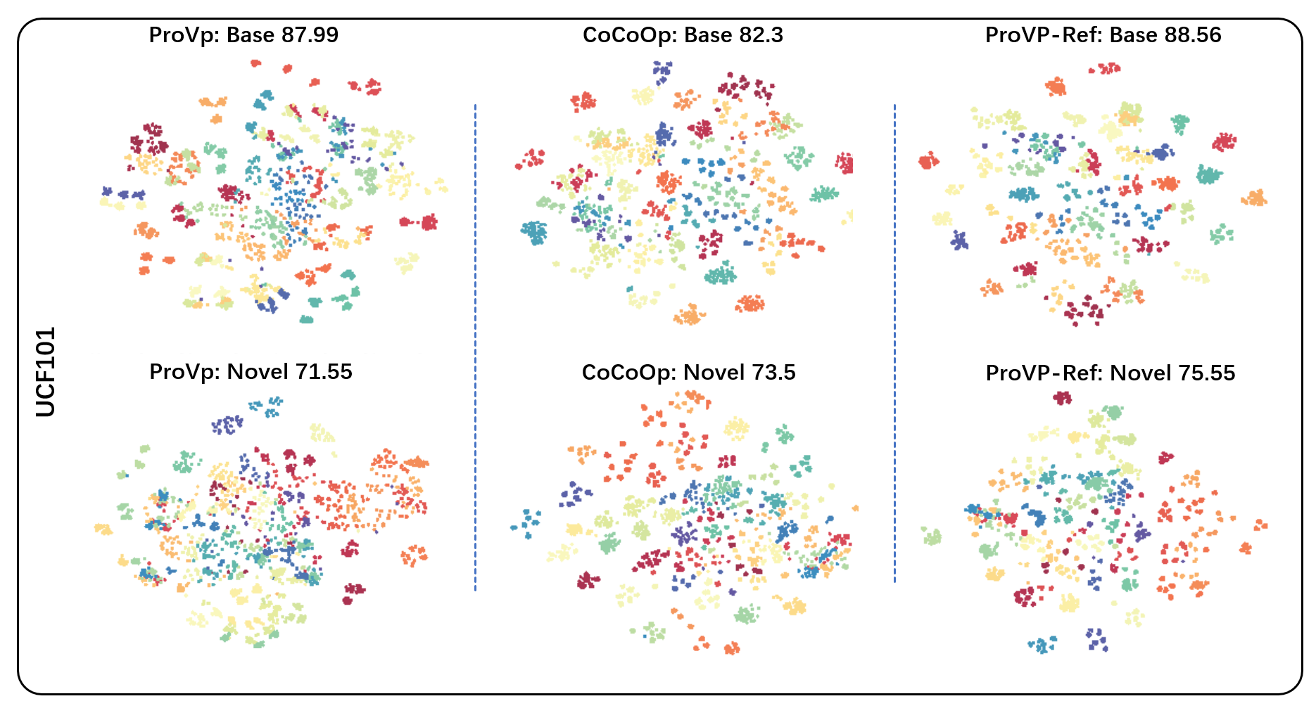
Figure 5: T-SNE plots of image embeddings in ProVP (left), CoCoOp (medium) and ProVP-Ref (right) on two diverse datasets. It is clear that the embeddings in ProVP and ProVP-Ref are more separable. Moreover, as ProVP-Ref has learned from the combination of pre-trained and downstream knowledge, it shares a more similar feature representation with zero-shot CLIP [33], which provides a better generalization capability.

Table 2: Comparison on the base-to-novel generalization setting. H: Harmonic mean of base and novel performance. Within all prompt-based methods, ProVP-Ref achieves the SOTA results on both base and novel classes.

(a) Average over 11 datasets.

	Base	Novel	H
CLIP	69.34	74.22	71.70
CoOp	82.69	63.22	71.66
CoCoOp	80.47	71.69	75.83
ProGrad	81.89	71.85	76.54
gray!15 ProVP	85.14	69.57	76.57
gray!15 ProVP_Ref	85.20	73.22	78.76

(b) ImageNet

	Base	Novel	H
CLIP	72.43	68.14	70.22
CoOp	76.47	67.88	71.92
CoCoOp	75.98	70.43	73.10
ProGrad	76.35	69.26	72.63
gray!15 ProVP	75.59	69.36	72.34
gray!15 ProVP_Ref	75.82	69.21	72.36

(c) Caltech101

	Base	Novel	H
CLIP	96.84	94.00	95.40
CoOp	98.00	89.81	93.73
CoCoOp	97.96	93.81	95.84
ProGrad	97.91	94.40	96.12
gray!15 ProVP	99.01	93.34	96.09
gray!15 ProVP_Ref	98.92	94.21	96.51

(d) OxfordPets

	Base	Novel	H
CLIP	91.17	97.26	94.12
CoOp	93.67	95.29	94.47
CoCoOp	95.20	97.69	96.43
ProGrad	94.86	97.52	96.17
gray!15 ProVP	95.80	96.18	95.99
gray!15 ProVP_Ref	95.87	97.65	96.75

(e) StanfordCars.

	Base	Novel	H
CLIP	63.37	74.89	68.65
CoOp	78.12	60.40	68.13
CoCoOp	70.49	73.59	72.01
ProGrad	75.17	74.37	74.77
gray!15 ProVP	80.97	63.27	71.03
gray!15 ProVP_Ref	80.43	67.96	73.67

(f) Flowers102.

	Base	Novel	H
CLIP	72.08	77.80	74.83
CoOp	97.60	59.67	74.06
CoCoOp	94.87	71.75	81.71
ProGrad	95.44	74.04	83.39
gray!15 ProVP	98.45	65.39	78.58
gray!15 ProVP_Ref	98.42	72.06	83.20

(g) Food101.

	Base	Novel	H
CLIP	90.10	91.22	90.66
CoOp	88.33	82.26	85.19
CoCoOp	90.70	91.29	90.99
ProGrad	90.73	91.27	91.00
gray!15 ProVP	90.16	90.88	90.52
gray!15 ProVP_Ref	90.32	90.91	90.61

(h) FGVCAircraft.

	Base	Novel	H
CLIP	27.19	36.29	31.09
CoOp	40.44	22.30	28.75
CoCoOp	33.41	23.71	27.74
ProGrad	38.88	31.63	34.88
gray!15 ProVP	46.04	25.29	32.65
gray!15 ProVP_Ref	47.08	29.87	36.55

(i) SUN397.

	Base	Novel	H
CLIP	69.36	75.35	72.23
CoOp	80.60	65.89	72.51
CoCoOp	79.74	76.86	78.27
ProGrad	80.85	74.93	77.78
gray!15 ProVP	80.33	73.75	76.90
gray!15 ProVP_Ref	80.67	76.11	78.32

(j) DTD.

	Base	Novel	H
CLIP	53.24	59.90	56.37
CoOp	79.44	41.18	54.24
CoCoOp	77.01	56.00	64.85
ProGrad	77.16	54.63	63.97
gray!15 ProVP	84.76	52.82	65.08
gray!15 ProVP_Ref	83.95	59.06	69.34

(k) EuroSAT.

	Base	Novel	H
CLIP	56.48	64.05	60.03
CoOp	92.19	54.74	68.69
CoCoOp	87.49	60.04	71.21
ProGrad	88.91	53.75	67.00
gray!15 ProVP	97.46	63.47	76.88
gray!15 ProVP_Ref	97.12	72.91	83.29

(l) UCF101.

	Base	Novel	H
CLIP	70.53	77.50	73.85
CoOp	84.69	56.05	67.46
CoCoOp	82.33	73.45	77.64
ProGrad	84.49	74.52	79.19
gray!15 ProVP	87.99	71.55	78.92
gray!15 ProVP_Ref	88.56	75.55	81.54

4.2 Base-to-Novel Generalization

Base-to-Novel Generalization is a scenario for evaluating model generalizability in a zero-shot setting. The dataset is split into base and novel sets with no shared classes. The models are trained on base set only but tested on both base and novel sets.

The overall results are shown in Table 2. We have three key findings: 1) ProVP performs impressively well on base classes, which achieves the best results on 9 out of 11 datasets and outperforms the previous best method (CoOp) by 2.45% on average. 2) Contrastive Feature Reformation significantly alleviates the generalization deterioration, e.g., ProVP-Ref boosts the novel performance on almost all datasets and gives 3.65% improvement over ProVP (73.22% vs 69.57%). It surpasses the previous state-of-the-art (ProGrad) on novel performance by 1.37%. 3) ProVP-Ref obtains the state-of-the-art results on both base and novel performance simultaneously, giving the best Harmonic mean. Unlike other methods which may sacrifice the base performance for the novel, we provide the best capability and trade-off for adaptation and generalization.

Meanwhile, ProVP-Ref gave sub-optimal novel performance on StanfordCars, Flowers102 and FGVCAircraft. We found all these datasets have a common characteristic: the best novel is achieved by zero-shot CLIP while its base is far behind all other methods. One possible reason is the pre-trained knowledge of CLIP, which contributes to the novel performance, may conflict with the downstream tasks and be degraded after the tuning. It is worth noting that this problem exists in all prompt learning methods on these datasets, and despite this issue, ProVP-Ref still achieves a competitive Harmonic mean.

The visualization of tuned embeddings is given in Figure 5, showing that ProVP-Ref indeed gains a more separable and generalizable representation compared to others.

Table 3: Results for ablation study. Table 3(a) compares ProVP and VPT on the average results in base-to-novel generalization. Table 3(b), Table 3(c) are ablation study for progressive decay $\alpha$ and $Loss_{Ref}$ weight $\lambda$ on few-shot learning, respectively.

(a) ProVP vs. VPT in base-to-novel.

Methods	Base	Novel	H
VPT-Shallow	80.06	72.35	76.01
VPT-Sha-Ref	79.45	72.70	75.93
VPT-Deep	84.97	68.74	76.00
VPT-Deep-Ref	84.85	71.50	77.60
gray!15 ProVP	85.14	69.57	76.57
gray!15 ProVP-Ref	85.20	73.22	78.76

(b) Different $\alpha$ in few-shot learning.

$\alpha$	Caltech101	DTD	StanfordCars
0.01	96.55	73.29	82.88
0.1	96.63	73.62	84.85
0.3	96.63	72.48	83.43
0.5	96.39	70.57	80.05
0.7	95.53	67.06	75.63
0.9	95.27	61.96	69.04

(c) Different $\lambda$ in few-shot learning.

$\lambda$	Caltech101	DTD	StanfordCars
0.	96.50	73.70	84.68
0.2	96.63	73.80	84.70
0.4	96.73	73.70	84.71
0.6	96.73	73.60	84.53
0.8	96.62	73.68	84.55
1.0	96.63	73.62	84.64

Table 4: Different $\lambda$ in base-to-novel generalization.

$\lambda$	DTD			StanfordCars
	Base	Novel	H	Base	Novel	H
0	84.76	52.82	65.08	80.97	63.27	71.03
0.2	84.61	55.03	66.69	81.07	64.29	71.71
0.4	84.53	55.80	67.22	81.21	66.15	72.91
0.6	84.18	58.01	68.69	80.78	66.97	73.23
0.8	83.95	58.82	69.17	80.36	68.07	73.71
1.0	83.95	59.06	69.34	80.43	67.96	73.67

4.3 Ablation Study

ProVP vs. VPT

A thorough comparison of ProVP and VPT structures is presented in Figure 6 for few-shot learning and Table 3(a) for base-to-novel generalization. For few-shot learning, ProVP consistently outperforms VPT across all shot settings and shows a remarkable improvement on extreme low shot settings (e.g., in 1-shot, ProVP outperforms VPT-Deep by 4.17%). Furthermore, in base-to-novel generalization, the significant improvement in novel performance (+1.72% on average) also indicates the effectiveness of the instance-adaptive approach used in ProVP, which further improves the generalization capability.

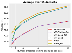
Figure 6: ProVP vs. VPT on few-shot learning. ProVP shows a consistent better performance.

The choice of $\mathbf{\alpha}$

We tested different $\alpha$ on three types of downstream datasets as Caltech101 [8] for general objects recognition, StanfordCars [18] for fine-grained classification and DTD [3], which have a large domain shift. The results are shown in Table 3(b). As $\alpha$ increases, the behavior of ProVP becomes closer to VPT-Shallow: the performance is still promising on Caltech101, but degrades on DTD and StanfordCars. It suggests that the adaptation ability is still determined by the new inserted prompts. In our experiment, we set $\alpha$=0.1 as it gave the best result.

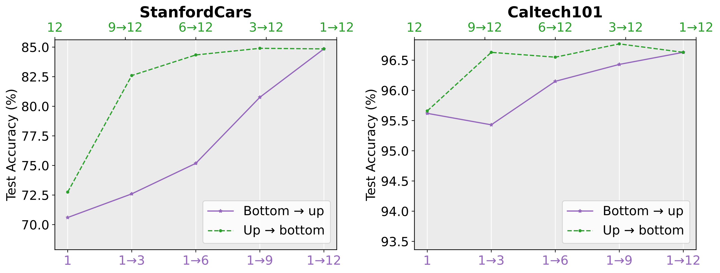
Figure 7: Ablation on prompt depth. $i\to j$ means the transformer layers inserted with prompts. Unlike VPT [17], prompts near output layers shows a more important impact on model performance.

The effect of Contrastive Feature Re-formation

As contrastive feature re-formation may behave differently in various tasks, we dig further on how $Loss_{Ref}$ in Eq. (6) affects the learning process of the models. A full ablation study is displayed in Table 3(c) for few-shot learning and Table 4 for base-to-novel generalization. As $\lambda$ increases, the novel performance of all datasets is consistently improved, which demonstrates the effectiveness of our method. Moreover, in Table 3(c) we found an appropriate $\lambda$ can enhance the transferring performance as well, which tells that maintaining knowledge via feature space is more flexible for prompt learning tasks (The best $\lambda$ may vary with different datasets).

Table 5: ProVP-Ref vs. text prompting with larger prompt length. The $x$ in model_x: the total prompt length in the model. Acc_fs: average accuracy in few-shot learning of 11 datasets. Base, Novel, H: average results in base-to-novel generalization.

Models	# params	Accfs	Base	Novel	H
CoOp60	30720	80.88	83.23	68.37	75.07
CoCoOp4+Mnet	34846	/	80.43	71.69	75.83
ProGrad60	30720	80.47	83.05	71.00	76.55
gray!15 ProVP-Ref48	36864	81.72	84.48	72.14	77.83
gray!15 ProVP-Ref60	46080	81.79	84.61	72.91	78.32

Questioning about parameters

Since our visual prompting method utilized more learnable prompts compared to text based methods, one may doubt that whether the larger parameter size is the key for such improvements. Thus, we decrease the prompt length of ProVP-Ref to reach the maximal size where CoOp and ProGrad can meet and the fair comparison is shown in Table 5. The results show that: larger parameters is not the reason for the gain of our models. Besides, our ProVP-Ref appears to be more scalable as it can benefit from more tunable prompts.

5 Conclusion

We propose a novel progressive structure for visual prompt learning in V-L models, which utilizes an instance adaptive manner to gain a more robust representation and a stable training process. Contrastive feature re-formation is further proposed to alleviate generalization deterioration problem. Combining both, ProVP-Ref outperforms all previous prompt-based methods and shows a significant stronger adaptation and generalization capability on two fundamental scenarios of few-shot learning. The advantage is more clear on the datasets with larger domain shifts. However, the intrinsic drawback of CLIP [33] bottlenecked the performance of our method when the number of labels increases. As such problems can be alleviated by using the learned text prompts, it exhibits the effectiveness of both visual and text prompt learning and lights a promising direction of how to optimize prompts of each modality interactively. We leave this for future work.

Appendix

Appendix A Additional Implementation Details

A.1 ProVP

The hyper-parameters for ProVP and ProVP-Ref are shown in Table 6. For few-shot learning, we use the same weight decay 0.0005 for all datasets. For base-to-novel generalization, we found that slightly increasing the weight decay could improve the performance on novel classes for several datasets, which is selected from [0.0005, 0.001]. In addition, a lager weight decay can also benefit the performance on ImageNet[5] where we set 0.005.

A.2 VPT variants

In terms of VPT-Deep and VPT-Shallow[17], for a fair comparison, the results in the original paper is not used in our paper due to 1) different pre-trained ViT (4M image-text vs 1.4M labelled images) and 2) different classifier (text encoder vs linear head) 3) different training samples. Therefore all VPT results in our paper are implemented by us with the same setting to ProVP. In terms of implementation details, we keep almost all the hyper-parameters as the same as ProVP and ProVP-Ref. For VPT-Shallow, we set the prompt length to 50, which is equal to the prompt length of ProVP in the first layer. We experimentally found that using the same learnable parameter size for VPT-Shallow (e.g., insert 50$\times$12=600 prompts in the first layer) was hard to optimize and performed poorly. Another difference is the weight decay of ImageNet in base-to-novel generalization. Although a larger weight decay would benefit the performance of ProVP, it would crash the training of VPT-Deep, and finally we set the weight decay to 0.001. Such results also indicate that our ProVP indeed has stabilized the training process.

A.3 other methods

In few-shot learning, following the original paper[51, 52], we optimize CoOp and ProGrad with the context prompt length set to 16. The maximal training epoch is set to 50 for 1 shot, 100 for 2/4 shots and 200 for 8/16 shots except ImageNet (the maximal epoch is fixed as 50 for all shots). The learning rate is set to 0.002. In base-to-novel generalization, although the context prompt length of CoOp and CoCoOp[50] is set to 4 in the original paper, it is not applicable for ProGrad as the prompts were initialized from the hand-crafted templates. To keep a fair comparison, we select from $[4,8,16]$ to find the minimal one which could fully cover the hand-crafted sentences.

Appendix B Additional Experiments

Table 6: The hyper-parameters for the proposed ProVP and ProVP-Ref. Prompt Length denotes the number of learnable prompts in each layer.

	Few-shot learning			Base-to-novel generalization
	Prompt Length	Weight Decay	$\lambda$	Prompt Length	Weight Decay	$\lambda$
ImageNet[5]	50	0.0005	0.1	16	0.005	0.1
Caltech101[8]	50	0.0005	1	16	0.0005	1
OxfordPets[30]	50	0.0005	1	16	0.001	1
StanfordCars[18]	50	0.0005	0.1	16	0.001	1
Flowers102[29]	50	0.0005	0.1	16	0.001	1
Food101[2]	50	0.0005	1	16	0.0005	1
FGVCAircraft[27]	50	0.0005	1	16	0.0005	1
SUN397[46]	50	0.0005	1	16	0.0005	1
DTD[3]	50	0.0005	1	16	0.001	1
EuroSAT[13]	50	0.0005	1	16	0.0005	1
UCF101[40]	50	0.0005	1	16	0.0005	1

Table 7: Complete Results for few-shot learning (Part I).

Methods		#Samples per class
		1	2	4	8	16
Average	CoOp	68.94	71.94	74.65	77.80	80.24
	ProGrad	70.68	72.87	75.48	77.88	79.84
	CLIP-Adapter	68.86	71.65	73.84	77.31	80.28
	VPT-Shallow	66.20	68.42	70.80	74.15	76.33
	VPT-Deep	67.20	72.42	75.43	79.04	82.59
	ProVP	70.86	73.44	76.57	79.77	82.96
gray!15	ProVP-Ref	71.37	74.03	76.73	79.88	83.07
ImageNet	CoOp	68.85 ± 0.15	69.70 ± 0.07	70.21 ± 0.19	71.21 ± 0.06	71.92 ± 0.13
	ProGrad	69.55 ± 0.17	69.93 ± 0.05	70.72 ± 0.17	71.46 ± 0.07	72.09 ± 0.13
	CLIP-Adapter	68.05 ± 0.14	68.53 ± 0.10	69.06 ± 0.15	70.54 ± 0.13	71.13 ± 0.02
	VPT-Shallow	68.03 ± 0.14	68.30 ± 0.19	68.74 ± 0.12	69.01 ± 0.11	69.18 ± 0.06
	VPT-Deep	40.98 ± 19.89	67.74 ± 0.07	68.88 ± 0.18	70.02 ± 0.06	70.94 ± 0.02
	ProVP	67.34 ± 0.29	68.10 ± 0.20	69.18 ± 0.03	70.12 ± 0.12	71.17 ± 0.11
gray!15	ProVP-Ref	67.29 ± 0.19	68.54 ± 0.00	69.25 ± 0.06	70.23 ± 0.10	71.14 ± 0.15
Caltech101	CoOp	93.90 ± 0.38	94.16 ± 0.49	94.54 ± 0.58	95.32 ± 0.19	95.89 ± 0.09
	ProGrad	93.35 ± 0.56	94.60 ± 0.29	95.13 ± 0.25	95.51 ± 0.15	96.02 ± 0.25
	CLIP-Adapter	93.34 ± 0.02	93.64 ± 0.14	94.04 ± 0.15	94.54 ± 0.17	94.96 ± 0.04
	VPT-Shallow	92.95 ± 0.10	93.56 ± 0.08	94.24 ± 0.20	94.98 ± 0.21	95.62 ± 0.00
	VPT-Deep	93.14 ± 1.12	94.21 ± 0.59	95.04 ± 0.25	95.86 ± 0.19	96.50 ± 0.07
	ProVP	93.85 ± 0.30	94.74 ± 0.16	95.41 ± 0.29	95.96 ± 0.34	96.50 ± 0.27
gray!15	ProVP-Ref	94.01 ± 0.45	95.09 ± 0.18	95.28 ± 0.11	95.86 ± 0.22	96.63 ± 0.17
OxfordPets	CoOp	90.86 ± 0.99	90.82 ± 1.17	93.25 ± 0.15	93.29 ± 0.10	93.73 ± 0.14
	ProGrad	92.19 ± 0.35	92.30 ± 0.23	93.32 ± 0.17	93.18 ± 0.20	94.16 ± 0.06
	CLIP-Adapter	89.80 ± 0.47	90.36 ± 0.54	91.51 ± 0.40	91.97 ± 0.25	92.23 ± 0.27
	VPT-Shallow	88.39 ± 0.71	90.53 ± 0.62	91.79 ± 0.51	92.74 ± 0.36	93.09 ± 0.07
	VPT-Deep	90.88 ± 0.65	91.14 ± 0.18	92.31 ± 0.52	92.54 ± 0.19	93.10 ± 0.09
	ProVP	90.89 ± 0.38	92.40 ± 0.15	92.66 ± 0.33	92.90 ± 0.46	93.26 ± 0.22
gray!15	ProVP-Ref	91.31 ± 0.43	92.31 ± 0.27	93.02 ± 0.14	93.27 ± 0.18	93.89 ± 0.33

Table 8: Complete Results for few-shot learning (Part II).

Methods		#Samples per class
		1	2	4	8	16
StanfordCars	CoOp	67.36 ± 0.89	70.62 ± 0.65	74.78 ± 0.64	78.95 ± 0.26	82.76 ± 0.26
	ProGrad	68.12 ± 0.37	72.31 ± 1.61	75.38 ± 0.71	78.98 ± 0.14	81.35 ± 0.25
	CLIP-Adapter	66.49 ± 0.22	68.08 ± 0.32	71.30 ± 0.80	75.71 ± 0.33	80.82 ± 0.12
	VPT-Shallow	64.90 ± 0.06	66.19 ± 0.36	67.15 ± 0.20	69.13 ± 0.41	70.60 ± 0.51
	VPT-Deep	64.81 ± 1.20	66.88 ± 0.59	69.24 ± 0.57	76.08 ± 0.60	82.79 ± 0.40
	ProVP	66.75 ± 0.16	68.42 ± 0.40	71.73 ± 0.62	77.40 ± 0.75	84.68 ± 0.27
gray!15	ProVP-Ref	66.72 ± 0.32	67.93 ± 0.58	71.57 ± 0.90	77.33 ± 0.47	84.85 ± 0.22
Flowers102	CoOp	77.55 ± 0.65	87.93 ± 0.15	91.92 ± 0.66	94.64 ± 0.54	96.91 ± 0.45
	ProGrad	81.24 ± 1.75	88.39 ± 0.71	91.73 ± 1.15	93.72 ± 0.27	95.33 ± 0.33
	CLIP-Adapter	77.70 ± 0.85	86.44 ± 0.42	91.15 ± 0.63	95.26 ± 0.21	96.96 ± 0.19
	VPT-Shallow	68.87 ± 0.63	74.87 ± 1.75	80.09 ± 1.17	88.01 ± 0.84	91.76 ± 0.38
	VPT-Deep	75.79 ± 1.17	84.43 ± 0.83	88.87 ± 0.32	95.48 ± 0.19	97.60 ± 0.23
	ProVP	78.36 ± 0.56	86.52 ± 0.58	91.30 ± 0.69	95.99 ± 0.27	97.99 ± 0.28
gray!15	ProVP-Ref	79.10 ± 0.62	86.11 ± 0.98	91.70 ± 0.80	95.89 ± 0.08	98.16 ± 0.25
Food101	CoOp	85.34 ± 0.45	85.72 ± 0.23	86.37 ± 0.22	86.68 ± 0.05	87.16 ± 0.08
	ProGrad	86.48 ± 0.13	86.90 ± 0.30	86.68 ± 0.42	87.18 ± 0.08	87.38 ± 0.09
	CLIP-Adapter	85.92 ± 0.01	86.10 ± 0.08	86.46 ± 0.04	86.75 ± 0.06	87.00 ± 0.01
	VPT-Shallow	85.24 ± 0.04	85.40 ± 0.16	85.70 ± 0.15	86.23 ± 0.09	86.72 ± 0.10
	VPT-Deep	83.34 ± 0.60	84.14 ± 0.63	84.54 ± 0.47	85.50 ± 0.13	86.62 ± 0.20
	ProVP	84.79 ± 0.48	85.22 ± 0.42	86.08 ± 0.15	86.45 ± 0.09	87.07 ± 0.08
gray!15	ProVP-Ref	84.76 ± 0.20	85.54 ± 0.05	86.13 ± 0.10	86.41 ± 0.08	87.00 ± 0.12
FGVCAircraft	CoOp	25.12 ± 1.42	26.95 ± 4.04	31.65 ± 1.73	38.78 ± 0.28	43.54 ± 0.81
	ProGrad	29.12 ± 0.97	30.53 ± 0.15	34.91 ± 0.82	38.70 ± 0.46	41.11 ± 0.60
	CLIP-Adapter	27.94 ± 0.76	28.92 ± 0.51	33.03 ± 0.48	38.90 ± 0.60	45.18 ± 0.40
	VPT-Shallow	24.40 ± 0.44	25.99 ± 0.26	27.21 ± 0.45	30.03 ± 0.21	32.56 ± 0.34
	VPT-Deep	26.58 ± 0.38	28.36 ± 0.98	35.42 ± 0.65	42.15 ± 1.29	53.94 ± 1.60
	ProVP	27.51 ± 0.13	29.54 ± 0.91	34.72 ± 0.59	42.46 ± 0.37	53.40 ± 0.42
gray!15	ProVP-Ref	28.02 ± 0.15	30.55 ± 1.19	34.40 ± 0.72	43.47 ± 0.56	53.18 ± 0.39
SUN397	CoOp	67.69 ± 0.45	69.38 ± 0.21	71.65 ± 0.25	73.65 ± 0.15	75.34 ± 0.16
	ProGrad	68.75 ± 0.14	70.60 ± 0.13	72.22 ± 0.49	73.87 ± 0.26	75.62 ± 0.19
	CLIP-Adapter	67.26 ± 0.20	65.08 ± 0.31	67.93 ± 0.06	71.61 ± 0.24	74.11 ± 0.07
	VPT-Shallow	65.92 ± 0.31	67.47 ± 0.22	68.41 ± 0.18	68.94 ± 0.17	69.67 ± 0.14
	VPT-Deep	63.53 ± 0.15	66.88 ± 0.16	68.43 ± 0.42	71.24 ± 0.16	74.38 ± 0.11
	ProVP	65.21 ± 0.51	67.27 ± 0.33	70.12 ± 0.31	72.22 ± 0.13	74.65 ± 0.18
gray!15	ProVP-Ref	66.09 ± 0.69	68.42 ± 0.18	70.27 ± 0.23	72.48 ± 0.19	74.72 ± 0.03
DTD	CoOp	49.96 ± 1.75	55.26 ± 1.36	60.34 ± 0.77	65.26 ± 0.52	69.35 ± 0.49
	ProGrad	52.64 ± 2.55	54.10 ± 1.02	59.79 ± 0.55	64.14 ± 1.24	68.86 ± 0.17
	CLIP-Adapter	47.42 ± 0.68	54.47 ± 0.24	60.79 ± 0.20	66.11 ± 1.52	71.24 ± 0.47
	VPT-Shallow	44.80 ± 0.70	47.26 ± 0.29	48.86 ± 1.05	56.32 ± 0.37	61.94 ± 0.27
	VPT-Deep	50.94 ± 1.68	56.17 ± 1.78	61.70 ± 1.08	67.20 ± 0.80	73.07 ± 0.82
	ProVP	51.12 ± 1.43	57.72 ± 0.98	63.04 ± 0.49	68.60 ± 0.18	73.70 ± 0.46
gray!15	ProVP-Ref	52.22 ± 1.75	57.23 ± 0.88	63.33 ± 0.32	68.42 ± 0.44	73.62 ± 0.16
EuroSAT	CoOp	59.69 ± 0.95	65.43 ± 0.51	69.01 ± 0.47	76.71 ± 2.72	83.91 ± 1.47
	ProGrad	62.66 ± 2.13	66.07 ± 1.89	71.91 ± 4.99	79.14 ± 2.58	84.30 ± 1.85
	CLIP-Adapter	62.74 ± 3.13	71.61 ± 2.42	68.81 ± 2.92	78.09 ± 3.71	85.78 ± 0.87
	VPT-Shallow	56.28 ± 2.61	62.96 ± 7.65	73.32 ± 4.37	84.05 ± 1.15	90.59 ± 0.42
	VPT-Deep	77.26 ± 5.00	82.77 ± 3.57	87.72 ± 2.18	91.59 ± 0.26	93.81 ± 0.44
	ProVP	80.47 ± 1.57	84.41 ± 2.04	89.41 ± 1.03	91.76 ± 1.32	94.00 ± 0.42
gray!15	ProVP-Ref	82.88 ± 1.15	86.57 ± 2.09	88.97 ± 1.42	91.78 ± 0.39	94.19 ± 0.43
UCF101	CoOp	72.02 ± 1.52	75.41 ± 0.77	77.44 ± 0.44	81.35 ± 0.61	82.11 ± 0.35
	ProGrad	73.33 ± 0.39	75.88 ± 0.45	78.44 ± 0.30	80.75 ± 0.19	82.00 ± 0.24
	CLIP-Adapter	70.76 ± 0.33	74.87 ± 0.68	78.17 ± 0.81	80.89 ± 0.97	83.69 ± 1.15
	VPT-Shallow	68.44 ± 0.58	70.05 ± 0.39	73.25 ± 0.48	76.24 ± 0.83	77.91 ± 0.16
	VPT-Deep	71.97 ± 0.78	73.91 ± 0.49	77.61 ± 0.28	81.73 ± 0.16	85.72 ± 0.58
	ProVP	73.43 ± 0.77	74.52 ± 0.27	79.34 ± 0.66	83.83 ± 0.49	86.56 ± 0.80
gray!15	ProVP-Ref	72.72 ± 1.05	76.07 ± 0.15	80.13 ± 0.83	83.57 ± 0.54	86.43 ± 0.04

B.1 few-shot learning

Alleviate the hard training process.

As we stressed that ProVP could alleviate the oscillation of performance and sensitivity to hyper-parameters existed in VPT-Deep, Figure 8 is provided which shows the test accuracy of VPT-Deep and ProVP during training. The results demonstrate that our ProVP indeed gains a much more stable tuning.

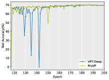
Figure 8: An example for the test accuracy of VPT-Deep and ProVP during training. ProVP shows a much more stable training process.

Table 9: Additional comparison in base-to-novel generalization.

		ImageNet	Caltech101	OxfordPets	StanfordCars	Flowers102	Food101	FGVCAircraft	SUN397	DTD	EuroSAT	UCF101	Average
Base	CLIP-Adapter	75.43	98.24	93.14	77.55	97.85	89.04	42.24	80.44	81.64	91.60	86.28	83.04
	VPT-Shallow	73.75	98.00	94.90	68.93	92.59	90.12	33.93	77.36	72.18	95.67	83.19	80.06
	VPT-Shallow-Ref	73.83	97.91	94.98	67.94	92.02	90.19	33.39	75.98	72.11	94.21	81.44	79.45
	VPT-Deep	76.20	98.97	95.82	79.06	98.42	90.24	44.42	80.17	84.41	98.17	88.78	84.97
	VPT-Deep-Ref	75.71	98.75	95.80	79.08	98.07	90.26	45.18	80.82	83.83	97.69	88.16	84.85
	ProVP	75.59	99.01	95.80	80.97	98.45	90.16	46.04	80.33	84.76	97.46	87.99	85.14
	ProVP-KD	75.09	98.62	95.29	77.25	92.21	90.76	42.40	78.67	77.51	91.96	84.28	82.19
	ProVP-PA	75.72	98.86	96.07	81.29	97.59	90.54	45.18	80.86	82.41	96.91	88.09	84.87
gray!15	ProVP-Ref	75.82	98.92	95.87	80.43	98.42	90.32	47.08	80.67	83.95	97.12	88.56	85.20
Novel	CLIP-Adapter	68.77	92.29	89.80	64.72	63.85	87.23	28.75	69.66	44.60	55.91	67.64	66.66
	VPT-Shallow	69.32	92.14	96.16	73.53	70.66	90.96	30.67	75.55	51.81	71.78	73.23	72.35
	VPT-Shallow-Ref	69.19	92.98	96.57	74.46	72.91	91.04	32.07	77.27	55.27	62.31	75.63	72.70
	VPT-Deep	66.57	92.68	95.83	64.87	63.03	90.80	27.41	74.36	54.03	57.72	68.80	68.74
	VPT-Deep-Ref	67.40	93.81	97.41	68.48	70.76	90.91	28.93	75.07	59.02	60.86	73.81	71.50
	ProVP	69.36	93.34	96.18	63.27	65.39	90.88	25.29	73.75	52.82	63.47	71.55	69.57
	ProVP-KD	69.41	93.74	97.34	72.92	75.51	90.34	31.27	76.76	62.60	60.88	76.67	73.40
	ProVP-PA	69.63	93.77	96.61	66.76	72.74	91.07	29.41	75.94	58.82	65.09	73.09	72.08
gray!15	ProVP-Ref	69.21	94.21	97.65	67.96	72.06	90.91	29.87	76.11	59.06	72.91	75.55	73.23
Harmonic Mean	CLIP-Adapter	71.95	95.17	91.44	70.56	77.28	88.13	34.21	74.66	57.69	69.44	75.83	73.95
	VPT-Shallow	71.47	94.98	95.53	71.16	80.15	90.54	32.22	76.44	60.32	82.02	77.89	76.01
	VPT-Shallow-Ref	71.43	95.38	95.77	71.05	72.91	90.61	32.72	76.62	62.58	75.01	78.43	75.93
	VPT-Deep	71.06	95.72	95.82	71.27	76.85	90.52	33.90	77.16	65.89	72.70	77.52	76.00
	VPT-Deep-Ref	71.31	96.22	96.60	73.40	82.21	90.58	35.27	77.84	69.27	75.00	80.35	77.60
	ProVP	72.34	96.09	95.99	71.03	78.58	90.52	32.65	76.90	65.08	76.88	78.92	76.57
	ProVP-KD	72.14	96.12	96.30	75.02	83.03	90.55	35.99	77.70	69.26	73.26	80.30	77.55
	ProVP-PA	72.55	96.25	96.34	73.31	83.35	90.80	35.63	78.32	68.64	77.87	79.89	77.95
gray!15	ProVP-Ref	72.36	96.51	96.75	73.67	83.20	90.61	36.55	78.32	69.34	83.29	81.54	78.76

Additional results.

The complete results for few-shot learning are shown in Table 7 and Table 8 where the results of CoOp[51], ProGrad[52], VPT[17] variants and ProVP are displayed in details. Furthermore, we also evaluated the CLIP-Adapter[9], an adapter-based method for few-shot learning which hires an extra feature extractor to learn from downstream datasets. The backbone of all methods is the open source CLIP[33] with ViT-B/16[6]. The average result of CLIP-Adapter is slightly better than CoOp and still far behind our ProVP-Ref. Moreover, we found that two visual-based methods (CLIP-Adapter and ProVP) neither perform well on ImageNet and SUN397. It also indicates that the bottleneck is caused by the low distinguishability of CLIP text features[35], which is described in the main paper. Compared to VPT variants, ProVP demonstrates two advantages: 1) recall the discarded prompt outputs, which could contain pre-trained knowledge and benefit the training process of extreme low shots setting; 2) strengthen the interaction between prompts of adjacent layers. The results of these two structures (Table 7 and Table 8) also indicates that ProVP shows a consistent improvement over VPT-Deep, especially on small shots settings.

B.2 base-to-novel generalization

Less appealing results in the main paper.

Explained in the main paper, we found particular datasets like StanfordCars and Flowers102 shows a sharper conflict in terms of the adaptation and generalization capabilities which brings a sub-optimal novel performance. A more banlanced result can also be produced if we choose to remain more general knowledge in the tuned model (e.g., shorter prompt length or lager $\lambda$ weight). A balanced version of StanfordCars is shown in Table 10, which implies a competitive novel performance can be also obtained by our approach. In the main paper we still provided the original results as we wanted to keep a fair comparison with consistent experimental settings.

Table 10: Balanced results on StanfordCars. The novel performance of such dataset is improved despite the decrease of the results on base classes.

	Base	Novel	H
ProVP-Ref (Default)	80.43	67.96	73.67
ProVP-Ref (Knowledge stressed)	75.5	73.3	74.38

Additional results.

In Table 9, we provide the detailed results of base-to-novel generalization, including CLIP-Adapter and VPT structures. Although Zhu et al. [52] have shown the methods applied in incremental learning are less efficient for prompt learning, we still evaluated our ProVP with the prompt aligned method proposed in [52] and the conventional knowledge distillation[23]. Specifically, ProVP-PA utilizes the method in [52] to align the gradient to not be conflict with the zero-shot predictions of CLIP, and ProVP-KD modifies the training loss as $Loss=Loss_{ce}+\beta*Loss_{KL}$, where $Loss_{KL}$ calculates the KL-divergence of the predicted logits of the tuned and pre-trained models (In our experiment, $\beta$ is set to 1 which is equal to our $\lambda$ setting). The results of such methods are also shown in Table 9. Notably, VPT-Shallow and ProVP-KD have a comparable performance with ProVP-Ref on novel classes, and ProVP-KD even obtains a marginally better result. However, the poor performance on base classes shows that such methods also have the problem that previous prompt-based methods faced with: the better generalization capability is likely to be a compromise of the insufficiency of downstream learning, and the gain on novel classes cannot compensate the loss of adaptation capability. For ProVP-PA, although it improves the results of ProVP, the performance drops on FGVCAircraft and DTD, which shows that ProVP-PA is still restricted by the incorrect predictions of zero-shot CLIP and may deteriorate when a large domain gap exists in the downstream dataset. Overcoming such drawback, ProVP-Ref still gains 1.15% over ProVP-PA on novel classes, showing a better generalization capability. Among all mentioned methods, ProVP-Ref obtains the best and the second best result on both base and novel classes, respectively. It demonstrates that our method balances the adaptation and generalization well and also implies that keeping the pre-trained knowledge via feature space is indeed more suitable for prompt learning on visual side.

References

- [1] Hyojin Bahng, Ali Jahanian, Swami Sankaranarayanan, and Phillip Isola. Exploring visual prompts for adapting large-scale models. arXiv preprint arXiv:2203.17274, 2022.
- [2] Lukas Bossard, Matthieu Guillaumin, and Luc Van Gool. Food-101–mining discriminative components with random forests. In ECCV, pages 446–461, 2014.
- [3] Mircea Cimpoi, Subhransu Maji, Iasonas Kokkinos, Sammy Mohamed, and Andrea Vedaldi. Describing textures in the wild. In CVPR, pages 3606–3613, 2014.
- [4] Marcos V Conde and Kerem Turgutlu. Clip-art: contrastive pre-training for fine-grained art classification. In CVPR, pages 3956–3960, 2021.
- [5] Jia Deng, Wei Dong, Richard Socher, Li-Jia Li, Kai Li, and Li Fei-Fei. Imagenet: A large-scale hierarchical image database. In CVPR, pages 248–255, 2009.
- [6] Alexey Dosovitskiy, Lucas Beyer, Alexander Kolesnikov, Dirk Weissenborn, Xiaohua Zhai, Thomas Unterthiner, Mostafa Dehghani, Matthias Minderer, Georg Heigold, Sylvain Gelly, et al. An image is worth 16x16 words: Transformers for image recognition at scale. In ICLR, 2021.
- [7] Yu Du, Fangyun Wei, Zihe Zhang, Miaojing Shi, Yue Gao, and Guoqi Li. Learning to prompt for open-vocabulary object detection with vision-language model. In CVPR, pages 14084–14093, 2022.
- [8] Li Fei-Fei, Rob Fergus, and Pietro Perona. Learning generative visual models from few training examples: An incremental bayesian approach tested on 101 object categories. In CVPR-W, pages 178–178, 2004.
- [9] Peng Gao, Shijie Geng, Renrui Zhang, Teli Ma, Rongyao Fang, Yongfeng Zhang, Hongsheng Li, and Yu Qiao. Clip-adapter: Better vision-language models with feature adapters. arXiv preprint arXiv:2110.04544, 2021.
- [10] Golnaz Ghiasi, Xiuye Gu, Yin Cui, and Tsung-Yi Lin. Scaling open-vocabulary image segmentation with image-level labels. In ECCV, pages 540–557, 2022.
- [11] Xavier Glorot and Yoshua Bengio. Understanding the difficulty of training deep feedforward neural networks. In AISTATS, pages 249–256, 2010.
- [12] Xiuye Gu, Tsung-Yi Lin, Weicheng Kuo, and Yin Cui. Open-vocabulary object detection via vision and language knowledge distillation. In ICLR, 2021.
- [13] Patrick Helber, Benjamin Bischke, Andreas Dengel, and Damian Borth. Eurosat: A novel dataset and deep learning benchmark for land use and land cover classification. IEEE Journal of Selected Topics in Applied Earth Observations and Remote Sensing, 12(7):2217–2226, 2019.
- [14] Geoffrey Hinton, Oriol Vinyals, and Jeff Dean. Distilling the knowledge in a neural network. arXiv preprint arXiv:1503.02531, 2, 2015.
- [15] Xinting Hu, Kaihua Tang, Chunyan Miao, Xian-Sheng Hua, and Hanwang Zhang. Distilling causal effect of data in class-incremental learning. In CVPR, pages 3957–3966, 2021.
- [16] Chao Jia, Yinfei Yang, Ye Xia, Yi-Ting Chen, Zarana Parekh, Hieu Pham, Quoc Le, Yun-Hsuan Sung, Zhen Li, and Tom Duerig. Scaling up visual and vision-language representation learning with noisy text supervision. In ICML, pages 4904–4916, 2021.
- [17] Menglin Jia, Luming Tang, Bor-Chun Chen, Claire Cardie, Serge Belongie, Bharath Hariharan, and Ser-Nam Lim. Visual prompt tuning. In ECCV, 2022.
- [18] Jonathan Krause, Michael Stark, Jia Deng, and Li Fei-Fei. 3d object representations for fine-grained categorization. In ICCV-W, pages 554–561, 2013.
- [19] Brian Lester, Rami Al-Rfou, and Noah Constant. The power of scale for parameter-efficient prompt tuning. In EMNLP, pages 3045–3059, 2021.
- [20] Boyi Li, Kilian Q Weinberger, Serge Belongie, Vladlen Koltun, and Rene Ranftl. Language-driven semantic segmentation. In ICLR, 2021.
- [21] Xiang Lisa Li and Percy Liang. Prefix-tuning: Optimizing continuous prompts for generation. In ACL, pages 4582–4597, 2021.
- [22] Yangguang Li, Feng Liang, Lichen Zhao, Yufeng Cui, Wanli Ouyang, Jing Shao, Fengwei Yu, and Junjie Yan. Supervision exists everywhere: A data efficient contrastive language-image pre-training paradigm. In ICLR, 2021.
- [23] Zhizhong Li and Derek Hoiem. Learning without forgetting. In ECCV, pages 614–629, 2016.
- [24] Xiao Liu, Kaixuan Ji, Yicheng Fu, Zhengxiao Du, Zhilin Yang, and Jie Tang. P-tuning v2: Prompt tuning can be comparable to fine-tuning universally across scales and tasks. arXiv preprint arXiv:2110.07602, 2021.
- [25] Yaoyao Liu, Yuting Su, An-An Liu, Bernt Schiele, and Qianru Sun. Mnemonics training: Multi-class incremental learning without forgetting. In CVPR, pages 12245–12254, 2020.
- [26] Yuning Lu, Jianzhuang Liu, Yonggang Zhang, Yajing Liu, and Xinmei Tian. Prompt distribution learning. In CVPR, pages 5206–5215, 2022.
- [27] Subhransu Maji, Esa Rahtu, Juho Kannala, Matthew Blaschko, and Andrea Vedaldi. Fine-grained visual classification of aircraft. arXiv preprint arXiv:1306.5151, 2013.
- [28] Ron Mokady, Amir Hertz, and Amit H Bermano. Clipcap: Clip prefix for image captioning. arXiv preprint arXiv:2111.09734, 2021.
- [29] Maria-Elena Nilsback and Andrew Zisserman. Automated flower classification over a large number of classes. In ICVGIP, pages 722–729, 2008.
- [30] Omkar M Parkhi, Andrea Vedaldi, Andrew Zisserman, and CV Jawahar. Cats and dogs. In CVPR, pages 3498–3505, 2012.
- [31] Mary Phuong and Christoph Lampert. Towards understanding knowledge distillation. In ICML, pages 5142–5151, 2019.
- [32] Chengwei Qin and Shafiq Joty. Continual few-shot relation learning via embedding space regularization and data augmentation. In ACL, pages 2776–2789, 2022.
- [33] Alec Radford, Jong Wook Kim, Chris Hallacy, Aditya Ramesh, Gabriel Goh, Sandhini Agarwal, Girish Sastry, Amanda Askell, Pamela Mishkin, Jack Clark, et al. Learning transferable visual models from natural language supervision. In ICML, pages 8748–8763, 2021.
- [34] Sylvestre-Alvise Rebuffi, Alexander Kolesnikov, Georg Sperl, and Christoph H Lampert. icarl: Incremental classifier and representation learning. In CVPR, pages 2001–2010, 2017.
- [35] Shuhuai Ren, Lei Li, Xuancheng Ren, Guangxiang Zhao, and Xu Sun. Rethinking the openness of clip. arXiv preprint arXiv:2206.01986, 2022.
- [36] Matthew Riemer, Ignacio Cases, Robert Ajemian, Miao Liu, Irina Rish, Yuhai Tu, and Gerald Tesauro. Learning to learn without forgetting by maximizing transfer and minimizing interference. In ICLR, 2019.
- [37] Sheng Shen, Liunian Harold Li, Hao Tan, Mohit Bansal, Anna Rohrbach, Kai-Wei Chang, Zhewei Yao, and Kurt Keutzer. How much can clip benefit vision-and-language tasks? In ICLR, 2021.
- [38] Hengcan Shi, Munawar Hayat, Yicheng Wu, and Jianfei Cai. Proposalclip: Unsupervised open-category object proposal generation via exploiting clip cues. In CVPR, pages 9611–9620, 2022.
- [39] Manli Shu, Weili Nie, De-An Huang, Zhiding Yu, Tom Goldstein, Anima Anandkumar, and Chaowei Xiao. Test-time prompt tuning for zero-shot generalization in vision-language models. arXiv preprint arXiv:2209.07511, 2022.
- [40] Khurram Soomro, Amir Roshan Zamir, and Mubarak Shah. Ucf101: A dataset of 101 human actions classes from videos in the wild. arXiv preprint arXiv:1212.0402, 2012.
- [41] Mingkang Tang, Zhanyu Wang, Zhenhua Liu, Fengyun Rao, Dian Li, and Xiu Li. Clip4caption: Clip for video caption. In ACM International Conference on Multimedia, pages 4858–4862, 2021.
- [42] Ashish Vaswani, Noam Shazeer, Niki Parmar, Jakob Uszkoreit, Llion Jones, Aidan N Gomez, Łukasz Kaiser, and Illia Polosukhin. Attention is all you need. Advances in neural information processing systems, 30:5998–6008, 2017.
- [43] Yabin Wang, Zhiwu Huang, and Xiaopeng Hong. S-prompts learning with pre-trained transformers: An occam’s razor for domain incremental learning. arXiv preprint arXiv:2207.12819, 2022.
- [44] Zhaoqing Wang, Yu Lu, Qiang Li, Xunqiang Tao, Yandong Guo, Mingming Gong, and Tongliang Liu. Cris: Clip-driven referring image segmentation. In CVPR, pages 11686–11695, 2022.
- [45] Zifeng Wang, Zizhao Zhang, Chen-Yu Lee, Han Zhang, Ruoxi Sun, Xiaoqi Ren, Guolong Su, Vincent Perot, Jennifer Dy, and Tomas Pfister. Learning to prompt for continual learning. In CVPR, pages 139–149, 2022.
- [46] Jianxiong Xiao, James Hays, Krista A Ehinger, Aude Oliva, and Antonio Torralba. Sun database: Large-scale scene recognition from abbey to zoo. In CVPR, pages 3485–3492, 2010.
- [47] Lu Yuan, Dongdong Chen, Yi-Ling Chen, Noel Codella, Xiyang Dai, Jianfeng Gao, Houdong Hu, Xuedong Huang, Boxin Li, Chunyuan Li, et al. Florence: A new foundation model for computer vision. arXiv preprint arXiv:2111.11432, 2021.
- [48] Xiaohua Zhai, Xiao Wang, Basil Mustafa, Andreas Steiner, Daniel Keysers, Alexander Kolesnikov, and Lucas Beyer. Lit: Zero-shot transfer with locked-image text tuning. In CVPR, pages 18123–18133, 2022.
- [49] Renrui Zhang, Rongyao Fang, Peng Gao, Wei Zhang, Kunchang Li, Jifeng Dai, Yu Qiao, and Hongsheng Li. Tip-adapter: Training-free clip-adapter for better vision-language modeling. arXiv preprint arXiv:2111.03930, 2021.
- [50] Kaiyang Zhou, Jingkang Yang, Chen Change Loy, and Ziwei Liu. Conditional prompt learning for vision-language models. In CVPR, pages 16816–16825, 2022.
- [51] Kaiyang Zhou, Jingkang Yang, Chen Change Loy, and Ziwei Liu. Learning to prompt for vision-language models. International Journal of Computer Vision, 130(9):2337–2348, 2022.
- [52] Beier Zhu, Yulei Niu, Yucheng Han, Yue Wu, and Hanwang Zhang. Prompt-aligned gradient for prompt tuning. arXiv preprint arXiv:2205.14865, 2022.