Fundamental Sensitivity Limits for non-Hermitian Quantum Sensors

Abstract

Considering non-Hermitian systems implemented by utilizing enlarged quantum systems, we determine the fundamental limits for the sensitivity of non-Hermitian sensors from the perspective of quantum information. We prove that non-Hermitian sensors do not outperform their Hermitian counterparts (directly couple to the parameter) in the performance of sensitivity, due to the invariance of the quantum information about the parameter. By scrutinizing two concrete non-Hermitian sensing proposals, which are implemented using full quantum systems, we demonstrate that the sensitivity of these sensors is in agreement with our predictions. Our theory offers a comprehensive and model-independent framework for understanding the fundamental limits of non-Hermitian quantum sensors and builds the bridge over the gap between non-Hermitian physics and quantum metrology.

Introduction.– Parallel with the rapid development in quantum technology, quantum metrology [1, 2, 3, 4] and quantum sensing [5, 6] are becoming one of the focuses in quantum science. Quantum sensors exploit quantum coherence or quantum correlations to detect weak or nanoscale signals and exhibit great advantages in accuracy, repeatability and precision. Recently, a number of sensing proposals utilizing novel properties of non-Hermitian physics [7, 8, 9] have been proposed and experimentally demonstrated. For example, non-Hermitian lattice systems with skin effect [10, 11] or non-reciprocity [12] have been suggested to realize enhanced sensing. Specifically, the divergence of the susceptibility near the exceptional point (EP) is exploited to realize enhanced sensing with arbitrary precision [13, 14, 15, 16] and it has been demonstrated using various classical (quasi-classical) physical systems [17, 18, 19, 20, 21] or quantum systems [22, 23]. While these early experiments claimed enhancements compared to conventional Hermitian sensors, subsequent theoretical work has cast doubt on these results [24, 25, 26, 27, 28], suggesting that the reported enhancements may not have fully taken into account the effects of noise. After taking into account the noise, some theoretical works show the enhancement in sensitivity provided by non-Hermitian sensors may disappear [24, 27]. However, other theoretical works have claimed that the enhancement can persist even in the presence of noise [25, 26]. While some recent experiments have demonstrated enhanced sensitivity despite the presence of noise [22, 21], others have shown no such enhancement [23]. Currently, the fundamental limitations imposed by noise on non-Hermitian sensors are still a topic of debate [29], and a definitive conclusion on whether the non-Hermitian physics is superior for sensing is still elusive.

In sensing schemes that rely on quantum systems, quantum noise always arises during the projective measurement of the parameter-dependent quantum state [30]. This noise originates from quantum mechanics and cannot be eliminated, leading to the fundamental sensitivity limit. Quantum metrology focuses on how to beat the standard quantum limit by employing quantum correlations, like entanglement or squeezing [2]. While non-Hermitian systems can serve as an effective description of open system dynamics in certain situations [31, 8], the decoherence and dissipation in open systems are detrimental to the useful quantum features required for metrology  [32, 33, 34, 35, 36]. Therefore, the sensitivity enhancement from non-Hermitian sensors, which can be embedded in open systems, is quite counter-intuitive. Various theoretical works have been devoted to analyze the effect from the noise  [24, 25, 26, 27, 28], however, these investigations usually require modeling the effect of noise and calculating the dynamics using tools such as the quantum Langevin equation, for specific sensing schemes and probe states. Here, we provide a general conclusion on the fundamental sensitivity limit from the perspective of quantum information [37], without the requirement to solve intricate non-unitary quantum dynamics and independent of specific noise forms, probe states, and measurement regimes. We unambiguously prove that the non-Hermitian quantum sensors do not surpass the ultimate sensitivity of their Hermitian counterparts and cannot achieve arbitrary precision in realistic experimental settings with finite quantum resources.

Sensitivity bound for unitary parameter encoding.–Quantum metrology or quantum parameter estimation is to estimate the parameter $\lambda$ from the parameter-dependent quantum state $\rho_{\lambda}$. One crucial step is to make measurements on the quantum state. The measurement can be described by a Hermitian operator $\Pi$, and the probability of obtaining the measurement outcome $\xi$, conditioned on the parameter $\lambda$, is $P(\xi|\lambda)=\text{Tr}(\Pi\rho_{\lambda})$. We can evaluate the classical Fisher information $\mathcal{I}_{\lambda}$ corresponding to this specific measurement as $\mathcal{I}_{\lambda}=\sum_{\xi}P(\xi|\lambda)\left(\frac{\partial\ln P(\xi|\lambda)}{\partial\lambda}\right)^{2}$,which reflects the amount of information about the parameter contained in the distribution of measurement outcomes. Meanwhile, the estimation uncertainty is given by $\delta^{2}\lambda=\left\langle\left(\frac{\lambda_{\text{est}}}{d\langle\lambda_{\text{est}}\rangle/d\lambda}-\lambda\right)^{2}\right\rangle$, where $\lambda_{\text{est}}$ is the estimated value when the number of probes ($N$) and the number of trials ($\nu$) are finite, while $\lambda$ is the true value of the parameter. For the unbiased estimator, we have $d\langle\lambda_{\text{est}}\rangle/d\lambda=1$. In fact, the classical Fisher information bounds the estimation uncertainty achievable in this specific measurement, which fulfills the so-called Cramér-Rao bound: $\delta\lambda\geq{1}/{\sqrt{\nu\mathcal{I}_{\lambda}}}$, where $\nu$ is the number of repetitions or trials. This bound can be attained asymptotically as $\nu\rightarrow\infty$. When it is optimized over all possible measurements, we can find the maximal value of the classical Fisher information, known as the quantum Fisher information (QFI) [38], $\mathcal{I}_{\lambda}\leq F_{\lambda}$. Accordingly, the ultimate precision of parameter estimation for a specific parameter-dependent quantum state can be determined using the quantum Cramér-Rao bound [39], $\delta\lambda\geq{1}/{\sqrt{\nu F_{\lambda}}}$. The QFI  can be determined as $F_{\lambda}=\text{Tr}[\rho_{\lambda}\mathcal{L}^{2}]$, where $\mathcal{L}$ is the symmetric logarithmic derivative defined by ${\partial\rho_{\lambda}}/{\partial\lambda}=(\mathcal{L}\rho_{\lambda}+\rho_{\lambda}\mathcal{L})/2$.

Usually, the parameter-dependent quantum state $\rho_{\lambda}$ is obtained through time evolution governed by the parameter-dependent Hamiltonian $\hat{H}_{\lambda}(t)$. To be more specific, with the parameter-independent initial state (probe state) $\rho_{0}$, the parameter encoding process can be described as $\rho_{\lambda}(t)=U_{\lambda}(0\rightarrow t)\rho_{0}U^{\dagger}_{\lambda}(0\rightarrow t)$, where the unitary time evolution operator $U_{\lambda}(0\rightarrow t)=\mathcal{T}e^{-i\int_{0}^{t}{\hat{H}_{\lambda}(s)ds}}$, with $\mathcal{T}$ being the time-ordering operator. In the case where the initial state is a pure state, $\rho(0)=|\Psi_{0}\rangle\langle\Psi_{0}|$, the QFI can be calculated as $F_{\lambda}(t)=4(\langle\Psi_{0}|h_{\lambda}^{2}(t)|\Psi_{0}\rangle-\langle\Psi_{0}|h_{\lambda}(t)|\Psi_{0}\rangle^{2})\equiv 4\text{Var}[h_{\lambda}(t)]|_{|\Psi_{0}\rangle}$, where the Hermitian operator $h_{\lambda}(t)\equiv iU_{\lambda}^{\dagger}(0\rightarrow t)\frac{\partial}{\partial\lambda}U_{\lambda}(0\rightarrow t)$ is called the transformed local generator [41, 42]. We have defined $\text{Var}[{\hat{A}}]|_{|\Psi\rangle}$ as the variance of the Hermitian operator ${\hat{A}}$ with respect to $|\Psi\rangle$. It satisfies $\text{Var}[\hat{A}]|_{|\Psi\rangle}\leq||\hat{A}||^{2}/4$ for arbitrary $|\Psi\rangle$ [43], where the seminorm is defined as $||\hat{A}||\equiv M_{A}-m_{A}$, with $M_{A}$ ($m_{A}$) being the maximum (minimum) eigenvalue of $\hat{A}$. Then it follows $F_{\lambda}(t)\leq||h_{\lambda}(t)||^{2}\equiv F_{\lambda}^{(c)}(t)$, where $F_{\lambda}^{(c)}(t)$ is defined as the channel QFI, corresponding to the maximum QFI achievable by optimizing over all possible probe states.

The triangle inequality for the seminorm of Hermitian operators [43] states that $||\hat{A}+\hat{B}||\leq||\hat{A}||+||\hat{B}||$. Using the definition of $h_{\lambda}$ and the Schrödinger equation $i\partial U_{\lambda}/\partial t=H_{\lambda}U_{\lambda}$, we can obtain $\frac{\partial h_{\lambda}}{\partial t}=U_{\lambda}^{\dagger}(0\rightarrow t)\frac{\partial H_{\lambda}(t)}{\partial\lambda}U_{\lambda}(0\rightarrow t)$. Thus, the transformed local generator can be explicitly represented as $h_{\lambda}(t)=\int_{0}^{t}{U_{\lambda}^{\dagger}(0\rightarrow s)\frac{\partial H_{\lambda}(s)}{\partial\lambda}U_{\lambda}(0\rightarrow s)ds}$. By applying the triangle inequality, we obtain $||h_{\lambda}(t)||\leq\int_{0}^{t}{\left|\left|U_{\lambda}^{\dagger}(0\rightarrow s)\frac{\partial H_{\lambda}(s)}{\partial\lambda}U_{\lambda}(0\rightarrow s)\right|\right|ds}=\int_{0}^{t}{\left|\left|\frac{\partial H_{\lambda}(s)}{\partial\lambda}\right|\right|ds}$, where we have used the fact that unitary transformations do not change the spectrum of an operator. Therefore, the upper bound of the channel QFI can be obtained as follows :

$$F_{\lambda}^{(c)}(t)\leq\left[\int_{0}^{t}\left|\left|\frac{\partial H_{\lambda}(s)}{\partial\lambda}\right|\right|ds\right]^{2}.$$ (1)

Due to the convexity of QFI, the optimal probe state is always a pure state [45]. Therefore, this bound is naturally applicable for mixed probe states. Similar relations [46, 45] have been obtained using different methods and have been employed to discuss unitary parameter encoding processes governed by Hermitian time-dependent Hamiltonians. Furthermore, by utilizing the quantum Cramér-Rao bound, we obtain the lower bound for the estimation uncertainty as follows :

$$\delta\lambda\geq\frac{1}{\sqrt{\nu}\int_{0}^{t}\left|\left|\frac{\partial H_{\lambda}(s)}{\partial\lambda}\right|\right|ds}.$$ (2)

Here, we realize that this relation is actually not limited to unitary parameter encoding processes. Instead, this bound can be applied to investigate non-unitary parameter encoding processes, particularly in the context of open quantum systems or dynamics governed by non-Hermitian Hamiltonians.

In this Letter, we proceed further to investigate the bound on the change rate of the QFI. By the definition of QFI, we obtain that $\frac{\partial F_{\lambda}}{\partial t}=8\left.\text{Cov}[\frac{\partial h_{\lambda}}{\partial t},h_{\lambda}]\right|_{|\Psi_{0}\rangle}$, where the covariance is defined as $\left.\text{Cov}[\hat{A},\hat{B}]\right|_{|\Psi\rangle}\equiv\frac{1}{2}\langle\Psi|\hat{A}\hat{B}+\hat{B}\hat{A}|\Psi\rangle-\langle\Psi|\hat{A}|\Psi\rangle\langle\Psi|\hat{B}|\Psi\rangle$. The covariance inequality deduced from the Cauchy-Schwarz inequality states that $\left|\text{Cov}[\hat{A},\hat{B}]\right|\leq\sqrt{\text{Var}(\hat{A})\text{Var}(\hat{B})}$. Applying this inequality, we find:

$$\left|\text{Cov}[\frac{\partial h_{\lambda}}{\partial t},h_{\lambda}(t)]|_{|\Psi_{0}\rangle}\right| \leq\sqrt{\text{Var}[U_{\lambda}^{\dagger}\frac{\partial H_{\lambda}}{\partial\lambda}U_{\lambda}]|_{|\Psi_{0}\rangle}}\frac{F_{\lambda}^{1/2}(t)}{2}$$ (3)

$$\leq\frac{||\frac{\partial H_{\lambda}}{\partial\lambda}||}{2}\frac{F_{\lambda}^{1/2}(t)}{2}.$$

After some algebra , we prove the following inequality:

$$\left|\frac{\partial F_{\lambda}^{1/2}(t)}{\partial t}\right|\leq\left|\left|\frac{\partial H_{\lambda}(t)}{\partial\lambda}\right|\right|.$$ (4)

Namely, the change rate of the square root of QFI is only bounded by the spectral width of the derivative of the Hamiltonian with respect to the parameter. $|{\partial F_{\lambda}^{1/2}(t)}/{\partial t}|$ measures how fast the quantum information about the parameter flows into or out of the quantum state. It indicates that the quantum parameter encoding process cannot be accelerated by adding auxiliary parameter-independent Hamiltonian extensions.

Open system and non-Hermitian quantum sensing.–In many situations, such as dynamics in open quantum systems or systems governed by non-Hermitian Hamiltonians, the dynamical process used to encode the parameter may be non-unitary. However, it is often possible to map these non-unitary processes to equivalent unitary dynamics in an enlarged Hilbert space, by introducing extra degrees of freedom that correspond to the environment [32]. We now make this statement more rigorous for non-unitary sensing schemes. Prior to applying the perturbation that incorporates the parameter to be estimated, the dynamical process in the open quantum system or non-Hermitian system, $R_{S}:\rho_{S}(0)\rightarrow\rho_{S}(t)$, can be mapped from a unitary evolution in an enlarged system, $\mathcal{M}(U_{S,E})\rightarrow R_{S}$. This unitary time evolution operator for the combined system corresponds to a Hermitian Hamiltonian, $U_{S,E}\rightarrow\tilde{H}_{\text{tot}}$. This Hamiltonian, $\tilde{H}_{\text{tot}}=H_{S}(t)+H_{E}(t)+H_{SE}(t)$, generally contains terms that describe the system $H_{S}(t)$, the environment $H_{E}(t)$ and the system-environment interaction $H_{SE}(t)$. Subsequently, we introduce the perturbation that incorporates the parameter dependence. In most scenarios, including the examples discussed in this work and various non-Hermitian sensing protocols, the parameter of interest directly couples to the degrees of freedom of the system and the perturbation can be represented by a Hermitian Hamiltonian $H_{1}(\lambda,t)$. As a result, the overall parameter encoding process, corresponding to the dynamical evolution in the open system or non-Hermitian system, can be mapped to a unitary dynamics governed by a Hermitian Hamiltonian $H_{\lambda}(t)=\tilde{H}_{\text{tot}}+H_{1}(\lambda,t)$. By mapping the dynamics to an enlarged system, we circumvent the analysis of intricate non-unitary parameter encoding processes. By resorting to the corresponding unitary evolution in the enlarged system, we can straightforwardly apply the ultimate sensitivity bound in Eq. (2) and the QFI rate bound in Eq. (4).

Since the estimation parameter only associates with the degree of freedom of the system, we have $\partial H_{\lambda}/\partial\lambda=\partial H_{1}/\partial\lambda$. Thus, the bounds in Eq. (2) and (4) reveal an intriguing insight: the ultimate sensitivity cannot be improved by coupling the system to the environment or by introducing auxiliary Hamiltonians. This is because these additional factors do not increase the amount of information about the parameter or the rate of information encoding. Correspondingly, the non-Hermitian sensor will not outperform its Hermitian counterpart in terms of ultimate sensitivity. We now substantiate this conclusion by analyzing some concrete examples.

Example I: single-qubit pseudo-Hermitian sensor.–A single-qubit pesudo-Hermitian  Hamiltonian, described by

$$\hat{H}_{s}=\mathcal{E}_{\lambda}\left(\begin{array}[]{ccc}0&\delta_{\lambda}^{-1}\\ \delta_{\lambda}&0\end{array}\right),$$ (5)

is employed to realize enhanced quantum sensing in Ref. [50], where $\mathcal{E}_{\lambda}$ and $\delta_{\lambda}$ depend on the parameter $\lambda$ that is being estimated. According to the Naimark dilation theory [51, 52], a dilated two-qubit system with a properly prepared initial state can be used to simulate the dynamics of this pseudo-Hermitian Hamiltonian, conditioned on the post-selection measurement of the ancilla qubit [53]. The Hermitian Hamiltonian of this dilated two-qubit system is

$$\hat{H}_{\text{tot}}=b\hat{I}^{(a)}\otimes\hat{\sigma}_{x}^{(s)}-c\hat{\sigma}_{y}^{(a)}\otimes\hat{\sigma}_{y}^{(s)}+\lambda\hat{I}^{(a)}\otimes\hat{\sigma}_{x}^{(s)},$$ (6)

where $\hat{\sigma}_{\alpha=x,y,z}^{(s)}$ ($\hat{\sigma}_{\alpha=x,y,z}^{(a)}$) represents the Pauli operators of the system qubit (ancilla qubit). The coefficients $b={4\omega\varepsilon(1+\varepsilon)}/{(1+2\varepsilon)}$ and $c={2\omega\sqrt{\varepsilon(1+\varepsilon)}}/{(1+2\varepsilon)}$, where $\varepsilon$ and $\omega$ describe the qubit. This specific dilated Hamiltonian can be mapped to $\hat{H}_{s}$, with $\mathcal{E}_{\lambda}=\sqrt{(b+\lambda)^{2}+c^{2}}$ and $\delta_{\lambda}={(\lambda+2\varepsilon\omega)}/{\mathcal{E}_{\lambda}}$. The time evolution of the quantum state governed by $\hat{H}_{s}$ is $|\psi\rangle_{s}=e^{-i\hat{H}_{s}t}|0\rangle_{s}=\cos(\mathcal{E}_{\lambda}t)|0\rangle_{s}-i\delta_{\lambda}\sin(\mathcal{E}_{\lambda}t)|1\rangle_{s}$. Thus the normalized population in $|0\rangle_{s}$ is $S(\lambda,t)={1}/{[1+\delta_{\lambda}^{2}\tan^{2}{(\mathcal{E}_{\lambda}t)}]}$. In Fig. 1(a), we plot the susceptibility $\chi_{s}(\lambda)\equiv\partial S/\partial\lambda$ as a function of $\lambda$ for a fixed evolution time $t=\tau\equiv{\pi}/{[4\omega\sqrt{\varepsilon(1+\varepsilon)}]}$. The result indicates that the maximal value of the susceptibility diverges as $\varepsilon\rightarrow 0$, which corresponds to the eigenstate coalescence. Based on this feature, the authors in Ref. [50] proposed the pseudo-Hermitian enhanced quantum sensing scheme.

On the other hand, for the dilated two-qubit system, the probe state should be prepared as $|\Psi_{0}\rangle=\left(\sqrt{\frac{1+\varepsilon}{1+2\varepsilon}}|0\rangle_{a}+\sqrt{\frac{\varepsilon}{1+2\varepsilon}}|1\rangle_{a}\right)\otimes|0\rangle_{s}$ in order to correctly simulate the non-Hermitian dynamics. The normalized population $S(\lambda,t)$ actually corresponds to the probability that the system qubit is in state $|0\rangle_{s}$, conditioned on the ancilla qubit being in state $|0\rangle_{a}$. Equivalently, by calculating the dynamics of the total system $|\Psi(\tau)\rangle=e^{-i\hat{H}_{\text{tot}}\tau}|\Psi_{0}\rangle$, we can directly evaluate the probability in state $|0\rangle_{a}\otimes|0\rangle_{s}$ as

$$P_{1}=\frac{1+\varepsilon}{1+2\varepsilon}\cos^{2}\left[t\sqrt{\lambda^{2}+\frac{8\varepsilon(1+\varepsilon)\lambda\omega}{1+2\varepsilon}+4\varepsilon(1+\varepsilon)\omega^{2}}\right].$$ (7)

Due to the quantum projection noise, there is uncertainty in the determination of $P_{1}$. This uncertainty originates from the quantum projective measurement and follows a binomial distribution. The variance of the estimated probability is $\text{Var}[\hat{P}_{1}]={P_{1}(1-P_{1})}/{\nu}$, where $\nu$ is the number of trials (repetitions) [48]. Using the error propagation formula, we can evaluate the estimation uncertainty for this specific sensing scheme as $\delta\lambda={\sqrt{\text{Var}[\hat{P}_{1}]}}/{|\frac{\partial P_{1}}{\partial\lambda}|}$. We plot the sensitivity in Fig. 1(b), which shows no divergence at the corresponding divergent positions of $\chi_{s}(\lambda)$ in Fig. 1(a). This absence of divergence in the sensitivity is attributed to the fact that the divergence in $\chi_{s}(\lambda)$ when $\varepsilon\rightarrow 0$ is accompanied by a vanishing success probability in the post-selection measurement. Namely, most experimental trails fail to provide useful information on the parameter. As a comparison, the counterpart Hermitian sensor simply employs $\hat{V}=\lambda\hat{I}^{(a)}\otimes\hat{\sigma}_{x}^{(s)}$ as the parameter encoding generator. The sensitivity bound in Eq. (2) indicates $\delta\lambda\geq\frac{1}{\sqrt{\nu}\tau||\hat{\sigma}_{x}||}=\frac{1}{2\sqrt{\nu}\tau}$. We plot this ultimate sensitivity bound in Fig. 1(b) as the blue lines, indicating that the non-Hermitian sensor does not outperform its Hermitian counterpart. Furthermore, the rate of dynamic QFI can be calculated exactly [48] as follows:

$$\frac{\partial F^{1/2}_{\lambda}(t)}{\partial t}=2\frac{\cos^{2}\theta+\sin^{2}\theta\frac{\sin{(2\Omega t)}}{2\Omega t}}{\sqrt{\cos^{2}\theta+\sin^{2}\theta\frac{\sin^{2}(\Omega t)}{(\Omega t)^{2}}}},$$ (8)

where we define $(b+\lambda)/\Omega=\cos\theta$ and $c/\Omega=\sin\theta$. It follows that $-2\leq\frac{\partial F^{1/2}_{\lambda}(t)}{\partial t}\leq 2$, which verifies our theory in Eq. (4).

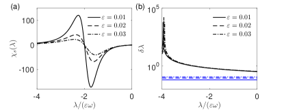
Figure 1: (a) Susceptibility of the normalized population with respect to $\lambda$ for different values of $\varepsilon$. It indicates that the maximal susceptibility diverges as $\varepsilon$ approaches zero. (b) Sensitivity corresponding to the measurement of the population in the state $|0\rangle_{a}\otimes|0\rangle_{s}$. It indicates that the sensitivity at the optimal measurement point (corresponding to the maximal susceptibility) does not diverge when $\varepsilon$ approaches zero. The blue lines represent the sensitivity bound of the Hermitian counterpart.

Example II: EP based sensor using a single trapped ion.–We now consider the sensor based on exceptional point realized in a dissipative single-qubit open system in Ref. [54]. The sensing mechanism relies on an effective periodically driven [55] $\mathcal{PT}$-symmetric non-Hermitian Hamiltonian given by

$$\hat{H}_{\mathcal{PT}}=J[1+\cos(\omega t)]\hat{\sigma}_{x}+i\Gamma\hat{\sigma}_{z},$$ (9)

where $\hat{\sigma}_{x,z}$ are the Pauli operators, $J$ is the coupling strength, $\omega$ is the modulation frequency of the coupling strength, and $\Gamma$ is the dissipation rate. Actually, the practically implemented Hamiltonian in the experiment is $\hat{H}_{\mathcal{PT}}^{\prime}=\hat{H}_{\mathcal{PT}}-i\Gamma\hat{I}$, which is a passive $\mathcal{PT}$-symmetric system with $\hat{I}$ being the identity operator. The perturbation applied to the system is $\hat{H}_{\delta}=\frac{\delta}{2}\cos(\omega_{\delta}t)(\hat{I}-\hat{\sigma}_{z})$, where $\delta$ and $\omega_{\delta}$ are the amplitude and frequency of the perturbation field, respectively, while $\omega_{\delta}$ is the parameter to be estimated. After the system evolves from specific initial states for a duration of $T=2\pi/\omega$, we can determine the response energy $\mathcal{E}_{\text{res}}$ via $P_{J}(T)-P_{\Gamma}(T)=\sin^{2}(\mathcal{E}_{\text{res}}T)$. Here, the measurable quantities are defined as $P_{J}(T)=\left|\left\langle\uparrow\right|U(T)\left|\downarrow\right\rangle\right|^{2}$ and $P_{\Gamma}(T)=\left|\frac{\left\langle\uparrow\right|-\left\langle\downarrow\right|}{\sqrt{2}}U(T)\frac{\left|\uparrow\right\rangle+\left|\downarrow\right\rangle}{\sqrt{2}}\right|^{2}$, with $U(T)=\mathcal{T}e^{-i\int_{0}^{T}{[\hat{H}_{\mathcal{PT}}(t)+\hat{H}_{\delta}(t)]dt}}$. The absolute value of the response energy $\mathcal{E}_{\text{res}}$ as a function of $\omega_{\delta}$ is plotted in Fig. 2(a) . As it is shown, the response energy exhibits sharp dips near the EP . This characteristic feature has motivated the authors in Ref. [54] to suggest the sensing application, since a minor change in $\omega_{\delta}$ will result in a significant variation in the response energy. Indeed, in Fig. 2(c), we present the susceptibility $|\partial\mathcal{E}_{\text{res}}/\partial\omega_{\delta}|$ as a function of $\omega_{\delta}$ and it exhibits a divergence near the EP.

However, the study in Ref. [54] has neglected effects from the quantum noise. Here, since $P_{J}$ and $P_{\Gamma}$ actually correspond to projective measurements on the spin state, the quantum projection noise will result in uncertainties in their determination. The variance of the estimated $\hat{P}_{J}$ and $\hat{P}_{\Gamma}$ can be expressed as $\text{Var}[\hat{P}_{i}]={P_{i}(C_{0}-P_{i})}/{\nu},\text{with }i=J,\Gamma$, where $\nu$ is the number of trials and $C_{0}\equiv e^{2\Gamma T}$ . To avoid the complication of dealing with complex response energies, we focus on the region near the EP where $P_{J}-P_{\Gamma}>0$. Applying the theory of uncertainty propagation, we obtain the uncertainty in the estimation of the response energy as $\text{Var}[\hat{\mathcal{E}}_{\text{res}}]=\frac{1}{4\nu T^{2}}\frac{C_{0}(P_{J}+P_{\Gamma})-(P_{J}^{2}+P_{\Gamma}^{2})}{(P_{J}-P_{\Gamma})(1-P_{J}+P_{\Gamma})}$, where we have used the fact that measurements on $P_{J}$ and $P_{\Gamma}$ are independent. We plot the variance of the measured response energy in Fig. 2(b) as a function of $\omega_{\delta}$, and it shows that the uncertainty in the determination of $\mathcal{E}_{\text{res}}$ also diverges when $\omega_{\delta}$ approaches the EP. The overall sensitivity can be evaluated as $\delta{\omega_{\delta}}={\sqrt{\text{Var}[\hat{\mathcal{E}}_{\text{res}}]}}/{|\frac{\partial\mathcal{E}_{\text{res}}}{\partial\omega_{\delta}}|}$, and we plot it in Fig. 2(d). It shows that the divergence of the susceptibility is completely compensated by the divergence of the uncertainty, resulting in an overall sensitivity without divergence when approaching the EP. On the other hand, the Hermitian counterpart simply uses $\hat{H}_{\delta}$ as the parameter encoding generator. According to Eq. (2), the ultimate sensitivity bound is given by $\delta{\omega_{\delta}}\geq\frac{\omega_{\delta}^{4}}{\sqrt{\nu}\delta^{2}[\sin(\omega_{\delta}T)-\omega_{\delta}T\cos(\omega_{\delta}T)]^{2}}$. The dashed line in Fig. 2(d) corresponds to this ultimate sensitivity bound. It also demonstrates that the ultimate precision of the Hermitian sensor always exceed the corresponding non-Hermitian sensor.

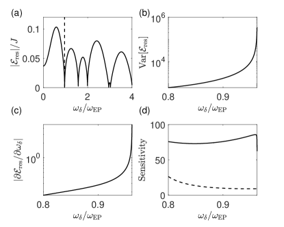
Figure 2: (a) Response energy shows sharp dips near the EP for the periodically driven non-Hermitian system. The dashed line indicates the position of the first EP. In (b-d), the range of $\omega$ corresponds to the zoom-ins of the left side of the first EP. (b) Variance of the response energy near the EP diverges. (c) Susceptibility of the response energy exhibit divergence near the EP. (d) The sensitivity, which is inversely proportional to the signal-to-noise ratio, shows no divergence. The dashed line represents the theoretical sensitivity bound of the Hermitian counterpart.

Summary and discussion.–In summary, we have unveiled the fundamental sensitivity limit for non-Hermitian sensors in the context of open quantum systems. Our results indicate clearly that non-Hermitian sensors do not outperform their Hermitian counterparts. In fact, when comparing the performance of quantum sensors, it is essential to fix the quantum resources consumed by these sensors. Actually, when resources are unlimited, even ideal Hermitian sensors can theoretically achieve arbitrary precision. However , in practical sensing scenarios, resources are always limited. The number of probes, sensing time, and the number of trials are examples of limited resources. As a result, achieving arbitrary precision is not possible in practical sensing scenarios. The aforementioned instances are characterized by a single probe. Notably, although these cases exhibit divergence in certain measurable quantities, it does not imply that the sensitivity diverges, leading to ‘arbitrary precision’, since the sensitivity of their Hermitian counterparts does not diverge (even without Heisenberg scaling for only $N=1$).

In Ref. [22], a sensing scheme utilizing an experimentally realized $\mathcal{PT}$-symmetric system was reported to enhance the sensitivity by a factor of 8.856 over a conventional Hermitian sensor. However, this enhancement is probably attributed to the choice of non-optimal initial probe state used for the Hermitian sensor, and similarly these seeming sensitivity enhancements in Refs. [25, 26] may not exist if making comparison over optimal probe states. Furthermore, non-Hermitian lattice systems utilizing the skin effect[10, 11] or the non-reciprocity [12], have claimed exponential scaling of sensitivity with the lattice size. However, our theory shows that the ultimate sensitivity should not depend on the lattice size, as it is solely determined by the subsystem dimension that directly couples to the parameter. Nevertheless, for non-optimal probe states or measurements, the sensitivity may still depend on the lattice size.

Although our work demonstrates that coupling to the environment cannot improve the ultimate sensitivity, when the probe state or the measurement protocol is restricted, adding appropriate auxiliary Hamiltonian may be helpful for approaching the ultimate sensitivity bound [59, 60, 61]. In fact, when the parameter couples to the environment, the bounds presented in Eq. (2) and (4) remain applicable, albeit $\partial H_{\lambda}/\partial\lambda$ now depends on the environment’s degrees of freedom. In addition, while our study focuses on non-Hermitian sensors implemented by full quantum systems [62, 63, 64], scrutinizing non-Hermitian sensors based on classical or quasiclassical systems [29] through the perspective of conservation of information is a compelling avenue for future research.