Mapping the distribution of OB stars and associations in Auriga

Abstract

OB associations are important probes of recent star formation and Galactic structure. In this study, we focus on the Auriga constellation, an important region of star formation due to its numerous young stars, star-forming regions and open clusters. We show using Gaia data that its two previously documented OB associations, Aur OB1 and OB2, are too extended in proper motion and distance to be genuine associations, encouraging us to revisit the census of OB associations in Auriga with modern techniques. We identify 5617 candidate OB stars across the region using photometry, astrometry and our SED fitting code, grouping these into 5 high-confidence OB associations using HDBSCAN. Three of these are replacements to the historical pair of associations - Aur OB2 is divided between a foreground and a background association - while the other two associations are completely new. We connect these OB associations to the surrounding open clusters and star-forming regions, analyse them physically and kinematically, constraining their ages through a combination of 3D kinematic traceback, the position of their members in the HR diagram and their connection to clusters of known age. Four of these OB associations are expanding, with kinematic ages up to a few tens of Myr. Finally, we identify an age gradient in the region spanning several associations that coincides with the motion of the Perseus spiral arm over the last $\sim$20 Myr across the field of view.

1 Introduction

First defined by Ambartsumian (1947), OB associations are gravitationally unbound groups of young stars containing bright O- and B-type stars. They have sizes from a few tens of parsecs to a few hundred parsecs and total stellar mass of one thousand to several tens of thousands of solar masses (Wright, 2020). They are valuable tracers of the distribution of young stars, and have been used for such purposes for decades (see e.g. Morgan et al. 1953 and Humphreys 1978). Most of the known OB associations are coincident with the Galactic spiral arms (Wright, 2020; Wright et al., 2022).

Bok (1934) pointed out that low-density systems were prone to disruption by tidal forces from the Galaxy, therefore Ambartsumian (1947) and Blaauw (1964) assumed that OB associations should be expanding. In the clustered model of star formation from Lada & Lada (2003), massive stars forming in embedded clusters disperse their parent molecular cloud by feedback, a process known as residual gas expulsion (Hills, 1980; Kroupa et al., 2001). With the majority of the mass of the system in the form of gas, embedded clusters unable to survive as gravitationally bound open clusters will expand and disperse as unbound OB associations. The hierarchical model of star formation, on the other hand, assumes that stars form over a range of densities, quickly decoupling from the gas in which they form. High-density clusters may survive as long-lived open clusters, while low-density groups will be gravitationally unbound from birth (Kruijssen, 2012). In such a model, OB associations may form gravitationally unbound and not require residual gas expulsion. Although the reality probably lies between these two cases (Wright, 2020), recent data and modern techniques can provide the key to unveil the origins of OB associations.

Expansion signatures from OB associations could indeed help to support the clustered model. Attempts to detect expansion in OB associations have had varied results, with early studies finding very little evidence for expansion (see e.g. Wright et al. 2016; Wright & Mamajek 2018; Ward & Kruijssen 2018), while later studies had more success (see e.g. Kounkel et al. 2018; Cantat-Gaudin et al. 2019; Armstrong et al. 2020; Quintana & Wright 2021). Failures to detect clear expansion signatures in OB associations have occurred mostly in systems with historically-defined membership (based on the position on the sky), while more recent studies that defined OB associations and their membership using spatial and kinematic information have proven more successful.

The Auriga constellation contains two OB associations identified and catalogued by Roberts (1972) and Humphreys (1978), as well as numerous young stars (Gyulbudaghian, 2011; Pandey et al., 2020), star-forming regions (Paladini et al., 2003; Mellinger, 2008; Anderson et al., 2015) and open clusters (Cantat-Gaudin & Anders, 2020). The Auriga constellation should intercept both the local arm and the Perseus spiral arm though few studies have focused on Galactic longitudes between 140^∘ and 180^∘ (Marco & Negueruela, 2016). Negueruela & Marco (2003) suggested the Auriga region is a less populated part of these spiral arms.

Aur OB1 is located at a distance of 1.06 kpc (Melnik & Dambis, 2020). It includes the open cluster NGC 1960 and the dark cloud LDN 1525 located at 1.2-1.3 kpc (Straižys et al., 2010), and is undergoing intense star formation (Panja et al., 2021).

Aur OB2 is located at a distance of 2.42 kpc (Melnik & Dambis, 2020). Its main features are the open clusters Stock 8, Alicante 11 and Alicante 12 (Marco & Negueruela, 2016). It was first thought that Aur OB2 extended between Stock 8 and NGC 1893, but recent studies have placed them at different distances, suggesting they may not all be part of the same system (Negueruela & Marco, 2003; Marco & Negueruela, 2016; Kuhn et al., 2019).

The paper is structured as follows. In Section 2 we revisit the historical Auriga OB associations with modern data and techniques. In Section 3 we outline our process for identifying OB stars, before detailing the clustering process used to identify new OB associations. In Section 4 we characterize these associations both physically and kinematically. In Section 5 we discuss the results in a broader context and we provide conclusions in Section 6.

2 The Auriga region

In this section we explore the existing OB associations in Auriga with modern photometry and astrometry from Gaia EDR3 (Gaia Collaboration et al., 2021), as well as any known open clusters and star-forming regions in their vicinity.

2.1 Historical OB associations

We focus our study on a 150 deg² area in the Auriga constellation, with $l$ = [165^∘, 180^∘] and $b$ = [-5^∘, 5^∘] as shown in Fig. 1. This area encompasses two historical associations, Aur OB1 and OB2. Their members have been listed in several catalogues (e.g. Humphreys 1978; Melnik & Dambis 2020). From Melnik & Dambis (2020) there are 36 stars in Aur OB1, 20 in Aur OB2 and 10 in NGC 1893, although only 6 of them have equatorial coordinates in Gaia EDR3 and listed in SIMBAD. NGC 1893 is usually considered part of Aur OB2 (see e.g. Marco & Negueruela 2016; Lim et al. 2018), and we follow that convention here, increasing the number of Aur OB2 members to 26 stars.

We match these 62 sources with Gaia EDR3 (Gaia Collaboration et al., 2021) using a radius of 1” and find a counterpart for all the stars. Following the criterion from Lindegren et al. (2021a), we only use the astrometry for the 48 stars whose renormalised united weight error (RUWE) is $<1.4$. Distances were taken from Bailer-Jones et al. (2021). The distribution of these stars in position, proper motions and distance is shown in Figs. 1, 2 and 3.

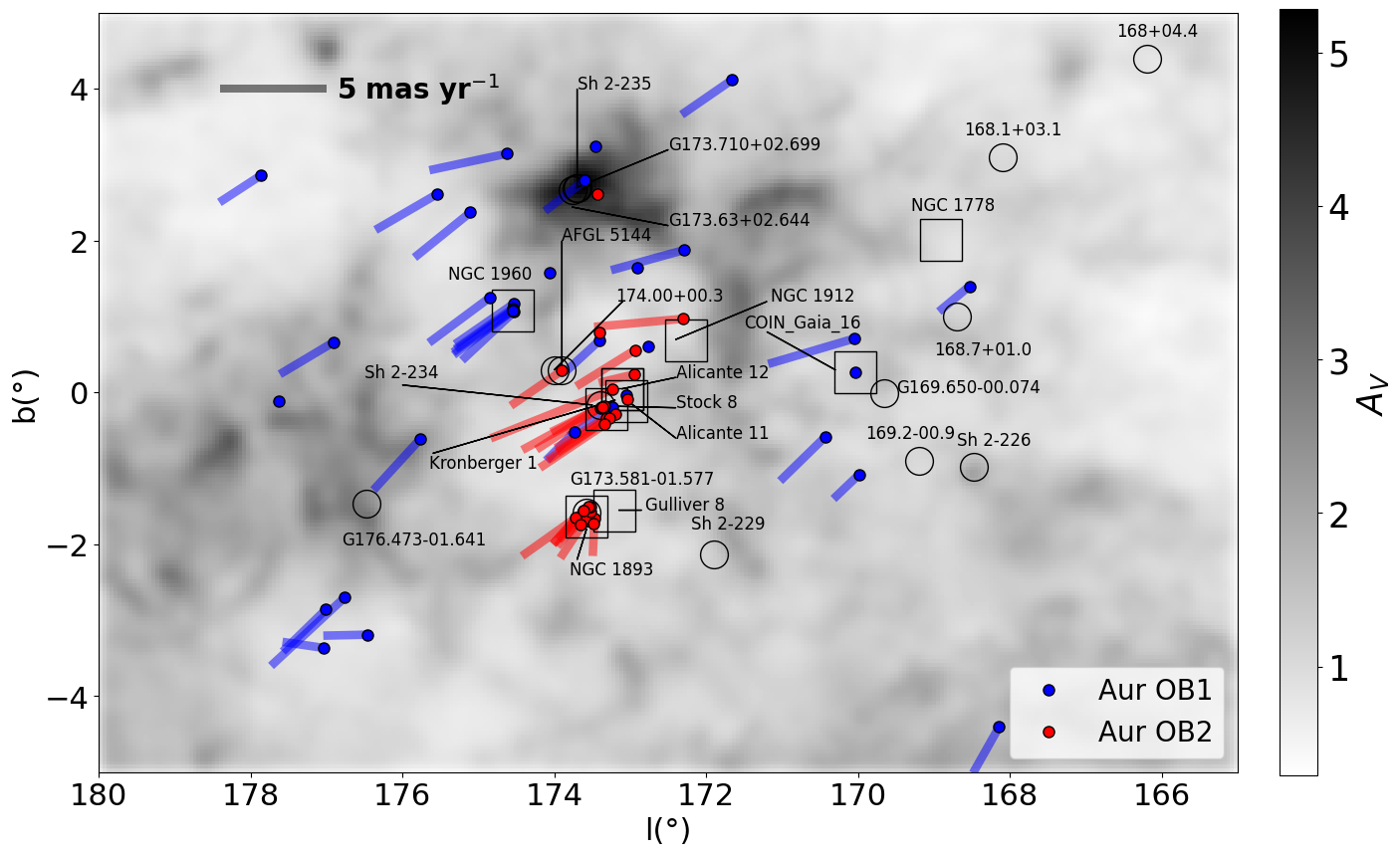
Figure 1: Spatial distribution in Galactic coordinates of the historical members of Aur OB1 and OB2. For the 48 stars with $RUWE<1.4$, their Galactic proper motions are represented as vectors (scale length indicated in the top left) while the stars without reliable proper motions are shown as points. We also show open clusters as empty squares (Cantat-Gaudin & Anders, 2020), and Hii and star-forming regions as empty circles (Paladini et al., 2003; Mellinger, 2008; Anderson et al., 2015). The background extinction map shows the integrated visual extinction at 2 kpc from Green et al. (2019).

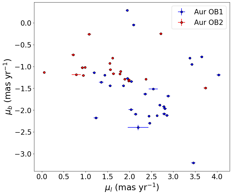
Figure 2: Proper motion distribution in Galactic coordinates for the historical members of Aur OB1 and OB2, with error bars, for stars with $RUWE<1.4$.

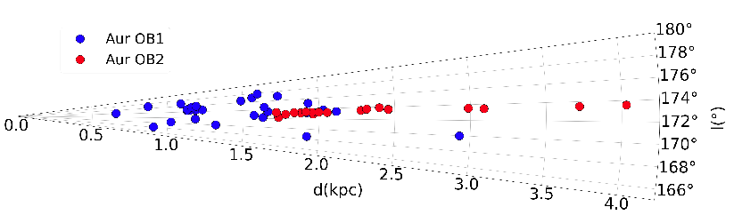
Figure 3: Galactic longitude plotted as a function of distances from Bailer-Jones et al. (2021) for the historical members of Aur OB1 and OB2 with $RUWE<1.4$.

Figures 1 and 2 show that the existing members of the two associations do not have a strong level of kinematic coherence, their proper motions each spread over 2-3 mas yr^-1 or 10-15 km s^-1 at 1 kpc, much larger than one would expect for an OB association (Wright, 2020). Figure 3 shows that the Aur OB1 members are spread over distances from 0.6 to > 2 kpc, much larger than the parallax uncertainties (typically 0.03 mas). A similar issue is apparent for Aur OB2, its members are spread from 1.7 to over 4 kpc, albeit with a core group of stars around 2 kpc, though this does not match with the distance to NGC 1893 of 2.9 kpc (Mel’Nik & Dambis, 2009; Melnik & Dambis, 2020). The presence of stars at distances of 3-4 kpc within these associations was previously noted by Marco & Negueruela (2016). OB associations have historically been defined through their on-sky spatial distribution and apparent magnitudes, with their members assumed to be within a narrow range of distances (see e.g. Humphreys 1978). It is clear that these two associations are not real OB associations; they neither exhibit the necessary kinematic coherence, nor are they located at a small enough range of distances to have been born together.

2.2 Open clusters and star-forming regions

To revisit our census of the OB associations in Auriga, we start by collating information on the known open clusters and star-forming regions in this area. Several tens of open clusters have been identified in the region (Cantat-Gaudin & Anders, 2020). In particular, five of them are likely related to the existing OB associations, following the discussions in Straižys et al. (2010), Marco & Negueruela (2016) and Pandey et al. (2020). The properties of these OCs are summarized in Table 1, where we have also included other OCs in the region whose relevance will be shown in Section 3.7. The clusters are also shown in Fig. 1 alongside the OB associations.

Table 1: Properties of the open clusters in Auriga thought to be related to the OB associations. Galactic coordinates and distances taken from Cantat-Gaudin & Anders (2020). References for the ages are: Jeffries et al. (2013) and Joshi et al. (2020) for NGC 1960, Marco & Negueruela (2016) for Stock 8, Alicante 11 and 12, Tapia et al. (1991), Marco et al. (2001), Sharma et al. (2007) and Lim et al. (2014) for NGC 1893, Subramaniam & Sagar (1999), Dias et al. (2021) for Gulliver 8, Jacobson et al. (2002), Pandey et al. (2007), Kharchenko et al. (2005) and Dib et al. (2018) for NGC 1912, Barbon & Hassan (1973), Kharchenko et al. (2013), Dib et al. (2018) and Cantat-Gaudin et al. (2020) for NGC 1778, Cantat-Gaudin et al. (2020) for COIN-Gaia_16 (here abbreviated CG16), Dib et al. (2018) and Cantat-Gaudin et al. (2020) for Kronberger 1 (here abbreviated K1).

OC	Assoc.	$l\,(\circ)$	$b\,(\circ)$	$d$ (kpc)	Age (Myr)
NGC 1960	Aur OB1	174.542	1.075	$1.16\pm 0.01$	18-26
Stock 8	Aur OB2	173.316	-0.223	$2.11\pm 0.01$	4-6
Alicante 11	Aur OB2	173.046	-0.119	$2.11\pm 0.01$	4-6
Alicante 12	Aur OB2	173.107	0.046	$2.11\pm 0.01$	4-6
NGC 1893	Aur OB2	173.577	-1.634	$3.37\pm 0.05$	1-5
Gulliver 8	-	173.213	-1.549	$1.11\pm 0.01$	22-39
NGC 1912	-	172.270	0.681	$1.10\pm 0.01$	250-375
NGC 1778	-	168.914	2.007	$1.64\pm 0.01$	150-282
CG16	-	170.038	0.270	$1.53^{+0.02}_{-0.01}$	26
K1	-	173.106	0.049	$2.12\pm 0.06$	6-8

In this area are also found multiple Hii regions (Paladini et al., 2003; Anderson et al., 2015), and several star-forming regions including Sh 2-235 and AFGL 5144 (Mellinger, 2008). They are shown in Fig. 1.

The most prominent feature of Fig. 1 is the centre of the region at $l\sim 173^{\circ}$ and $b\sim 0^{\circ}$. This is where the bulk of Aur OB2 members are located (Melnik & Dambis, 2020), along with the three open clusters Stock 8, Alicante 11 and 12 (see Table 1), and the Hii regions Sh 2-234 and 174.0+00.3. The star-forming region AFGL 5144 lies close to this area, at $l=173.7^{\circ}$ and $b=0.3^{\circ}$ (Mellinger, 2008), consistent with the young age of the OCs (Marco & Negueruela, 2016).

The star-forming region Sh 2-235 is located at $l=173.7^{\circ}$ and $b=2.7^{\circ}$ (Mellinger, 2008), close to the Hii regions G173.710+02.699 and G173.63+02.664, and where the region of highest extinction can be found (see Fig. 1).

3 Identification of new OB associations

In this section we summarize the method used to identify OB stars and associations. The method for identifying OB stars is very similar to that of Quintana & Wright (2021), which we briefly summarise here and highlight any changes.

3.1 Data and selection process

We utilise astrometry and optical photometry from Gaia EDR3 (Gaia Collaboration et al., 2021) , optical photometry from IGAPS (Drew et al., 2005; Monguió et al., 2020), and near-IR photometry from 2MASS (Cutri et al., 2003) and UKIDSS (Lucas et al., 2008). We require Gaia astrometry to have $RUWE<1.4$ and $|\frac{\varpi}{\sigma_{\varpi}}|>2$ , where $\varpi$ is the observed Gaia parallax and $\sigma_{\varpi}$ its random uncertainty. We limit our sample to stars with BP-RP < 2.5, a colour limit equivalent to a star with $\log(T_{\rm eff})=4$ and $A_{V}=6$, which is about the maximum extinction level in this region at a distance of 3 kpc (Green et al., 2019). The sources were filtered to have $d$ < 3.5 kpc, using the distances from Bailer-Jones et al. (2021).

Gaia photometry was required to have $|C^{*}|<3\,\sigma_{C*}$ where $C^{*}$ is the corrected excess flux factor in the $G_{\rm RP}$ and $G_{\rm BP}$ bands and $\sigma_{C*}$ is the power-law on the $G$ band with a chosen 3$\sigma$ level (Riello et al., 2021). 2MASS photometry was required to have a good quality flag (A, B, C or D, see Cutri et al. 2003) whilst those from UKIDSS had to fulfill $ErrBits<256$. For UKIDSS we also exclude photometry with either $J<13.25$, $H<12.75$ and $K<12$, below which the photometry risks saturation (Lucas et al., 2008). IGAPS photometry was filtered by excluding saturated photometric bands whose associated class did not indicate a star or probable star (Monguió et al., 2020). We then require at least one valid blue photometric band (either $g$, $G_{\rm BP}$ or $G$) and a valid near-infrared photometric band.

To remove faint (non-OB) stars, we then apply an absolute magnitude cut, requiring $M_{K}<1.07$ (if K-band photometry is available), $M_{H}<1.10$ (otherwise if H-band photometry is available), or $M_{J}<1.07$ (if only J-band photometry is available). These are the absolute magnitudes of main-sequence A0 stars (Pecaut & Mamajek, 2013).

Finally, the near-IR colour-colour diagram was used to remove background giants, as described in Quintana & Wright (2021).

This led to a working sample of 29,124 sources on which we applied our SED fitting process.

3.2 SED fitting

To calculate the physical properties of the sources, in order to identify OB stars, an SED fitting process was applied, based on the same method in Quintana & Wright (2021) with a few improvements, summarised here:

• We seek to estimate the model parameters log(Mass), Fr(Age), $d$ and $\ln(f)$ using the emcee package in Python (Foreman-Mackey et al., 2013). Fr(Age) is the fractional age (i.e. the age of a star divided by the maximum age at its initial stellar mass) and $\ln(f)$ is a scaling uncertainty to help the convergence of $\chi^{2}$ (Foreman-Mackey et al., 2013; Casey, 2016). $\log(T_{\rm eff})$ and $\log(L/L_{\odot})$ are indirect products of this process, and the extinction $A_{V}$ was derived using the 3D extinction map from Green et al. (2019) named Bayestar. The priors for these parameters are:

  $$\ln(P(\theta))=\begin{cases}\log(\frac{1}{2\,L^{3}}\,d^{2}\,\exp{(\frac{-d}{L}}))&\text{if }\begin{cases}-1.0\leq\log(\rm Mass)\leq 2.0\\ 0.0\leq\rm Fr(Age)\leq 1.0\\ 0.0\leq d\leq 5000.0\,\rm pc\\ -10.0\leq\ln(f)\leq 1.0\\ \end{cases}\\ -\infty&\text{otherwise}\end{cases}$$ (1)

  with the prior on distance from Bailer-Jones (2015) including a scale length $L$ set to 1.35 kpc.

• Our model SEDs use stellar spectral models (Werner & Dreizler, 1999; Rauch & Deetjen, 2003; Werner et al., 2003; Coelho, 2014), with a fixed value of $\log g=4$ and evolutionary models from Ekström et al. (2012). Model spectra were reddened using the Fitzpatrick et al. (2019) extinction laws and convolved with the relevant filter profiles to derive synthetic magnitudes.

• Systematic uncertainties were added to the measured photometric uncertainties. This is equal to 0.03 mag for $g$, $r$ and $i$ (Barentsen et al., 2014; Drew et al., 2014), 0.01 mag for $G$, $G_{\rm RP}$, $G_{\rm BP}$ (Riello et al., 2021), 0.03 mag for $J_{\rm 2M}$, 0.02 for $H_{\rm 2M}$ and $K_{\rm 2M}$ (Skrutskie et al., 2006), and 0.03 mag for $J_{\rm U}$, $H_{\rm U}$, $K_{\rm U}$ (Hodgkin et al., 2009).

• We choose the median value of the posterior distribution. The posterior distribution was explored using a Markov Chain Monte Carlo simulation. This utilised 1000 walkers, 200 burn-in iterations and 200 iterations. If the $\ln(f)$ value was greater than 4, or the difference between the 95th and 5th percentile of $\log(T_{\rm eff})$ was greater than 0.5 (indicating a lack of convergence), we ran 1000 supplementary burn-in and 200 supplementary iterations, until convergence was achieved or for 6000 supplementary burn-in iterations.

In addition, the extinctions from Gaia DR3 (Creevey et al., 2022; Delchambre et al., 2022) reveal that the Bayestar extinctions tend to be underestimated by $\sim$22 %. Instead of using the Gaia DR3 extinctions (due to their incomplete coverage of the Galactic plane, Delchambre et al. 2022), we increase the Bayestar extinctions by 22 per cent to compensate.

3.3 General results

SED fits were performed for all 29,124 candidate OB stars. Histograms of fitted physical parameters are shown in Fig. 4. There are 5434 stars with $\log(T_{\rm eff})>4$ (OB stars, 18.66 %) and 115 stars with $\log(T_{\rm eff})>4.3$ (O stars, 0.39 %). The median value of $\log(M/M_{\odot})$ is equal to 0.31 (with a standard deviation of 0.12 dex) while the median value of $\log(L/L_{\odot})$ is 1.43 (with a standard deviation of 0.44 dex). Most of the stars are located within 4 kpc (consistent with our selection from Bailer-Jones et al. 2021) with an increasing number at larger distances (as we probe a larger volume), while the peak of reddening is located at 1.5 mag, with the bulk at $A_{V}<3$ mag.

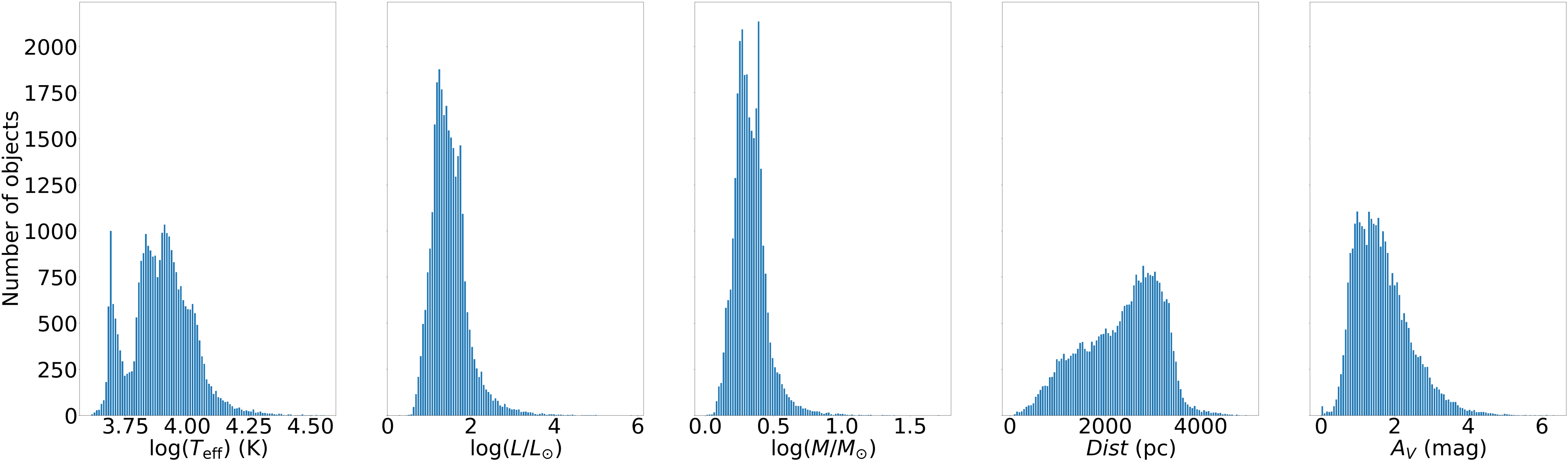
Figure 4: Median fitted parameters for the 29,124 selected sources of the working sample.

3.4 Incompleteness

Incompleteness in the working sample stems from the selection process. To estimate it, we compute the fraction of stars as a function of magnitude which were trimmed during the successive steps of Section 3.1. These steps include the removal of bad astrometric solutions (2-parameter sources, large error on parallaxes and large $RUWE$), the removal of bad photometry (blue or NIR) and high BP-RP values. A plot of the completeness level as a function of $G$ is shown in Fig. 5 for the SED-fitted OB stars (stars with $\log(T_{\rm eff})>4$ or $\log(L/L_{\odot})>2.5$).

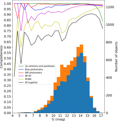
Figure 5: Completeness as a function of $G$ for the 5617 SED-fitted OB stars in the sample divided according to the different steps used to trim the sample. The black curve represents the product of all completeness curves. The blue and orange histograms show the number of sources before (blue) and after (orange) the completeness correction is applied.

To further verify the completeness of our sample, we crossmatch it with the OBA stars from Zari et al. (2021). Their list contains 14,973 stars in the Auriga region and from the 29,124 stars in our sample, there are 4818 stars in common, including 4097 with a SED-fitted $T_{\rm eff}$ greater than 8000 K (the minimum temperature for Zari et al. 2021). Unsuccessful matches for our list are due to a different $M_{K}$ threshold (we chose $M_{K}$ < 1.07 while they selected stars with $M_{K}$ < 0). Unsuccessful matches from their list are due to our selection process (e.g. we discarded distant stars that they kept). As we estimated the incompleteness due to our selection process (Fig. 5), this comparison shows that we have reached good completeness in probing the population of OB stars in Auriga.

3.5 Comparison with spectroscopic temperatures

To check the quality of the results, we build a sample of spectroscopic temperatures that we compare to our SED-fitted temperatures, by cross-matching our sample within 1 arcsec with two catalogues:

• Stars with spectral types from SIMBAD, filtered by removing sources with a quality measurement on spectral type of ’D’ and ’E’, along with those without an indicated spectral type and subclass. We then convert the spectral types into effective temperatures using the tabulations from Martins et al. (2005) for the O-type stars (observed scale), from Trundle et al. (2007) for early B-type stars, from Humphreys & McElroy (1984) for late B-type stars of luminosity classes ’I’ or ’III’ and from Pecaut & Mamajek (2013) for the later spectral types. We set a luminosity class of ’V’ when unspecified and chose error bars of one spectral subclass, whilst using the spectral type of the primary star for binaries and interpolating for luminosity classes of ’II’ and ’IV’.

• Stars from APOGEE DR17 (García Pérez et al., 2016; Abdurro’uf et al., 2022), selecting the sources with a measured $T_{\rm eff}$ from the pipeline and removing those with a warning on $T_{\rm eff}$ that are considered unreliable due to their proximity to the upper limit of APOGEE measurements (20,000 K).

We combine 70 stars from SIMBAD with 331 stars from APOGEE, making a sample of 397 unique stars (we use the weighted mean to calculate the temperature for the 4 stars in common). Our SED-fitted temperatures are compared with the spectroscopic temperatures in Fig. 6.

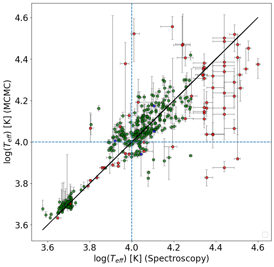
Figure 6: Comparison between the spectroscopic and SED-fitted temperatures for the 397 stars in the Auriga sample. Stars coloured in green are from APOGEE, stars coloured in red are from SIMBAD and stars coloured in blue are in both samples.

Choosing thresholds on $\log(T_{\rm eff})$ > 4 (4.1, 4.2 and 4.3), we define the recovery rate ${\rm RR}={\rm TP}/({\rm TP}+{\rm FN})$ where TP is the number of true positives (where both the SED-fitted and spectroscopic temperatures are above the threshold for selection of an OB star) and FN the number of false negatives (where the SED-fitted temperature is below the threshold and the spectroscopic temperature above). We also define the contamination rate, ${\rm CR}={\rm FP}/({\rm TP}+{\rm FP})$, where FP is the number of false positives (where the SED-fitted temperature is above the threshold and the spectroscopic temperature below). For these thresholds, RR is equal to 88% (80%, 56%, 49% ) and CR is between 17 and 30 %. These results suggest we are better at fitting late B-type stars, which could be due to the sparsity of very hot stars in this region, the high multiplicity of such stars (as our SED fitting code currently models all stars as single stars) or the high uncertainty on spectroscopic temperature of many of the O stars.

Fig. 6 also shows that our SED-fitted temperatures are in better agreement with the APOGEE spectroscopic temperatures than they are with the SIMBAD spectroscopic temperatures (which constitute most of the O-type stars). APOGEE spectra are generally more consistent and of better quality than the spectroscopy from SIMBAD, which might explain the difference. The median error on $T_{\rm eff}$ for the APOGEE spectroscopy is only $\sim$ 200 K, to be contrasted with $\sim$ 1100 K for the SIMBAD spectroscopic sample.

3.6 Clustering analysis with HDBSCAN

In Quintana & Wright (2021), we identified kinematically-coherent OB associations in the Cygnus region by applying a flexible clustering method based on a Kolmogorov-Smirnov (KS) test on Galactic coordinates and proper motions. This choice was feasible because the OB associations were all at a similar distance. The distance spread of the OB stars in Auriga, on the other hand, is much larger.

For this work we therefore use the Hierarchical Density-Based Spatial Clustering of Applications with Noise (HDBSCAN, McInnes et al. 2017) tool. It constitutes an extension of DBSCAN and identifies clusters by defining their cores through the number of neighbours within a radius $\epsilon$. In many clustering algorithms, including DBSCAN, the selection of clusters depends heavily upon the value of $\epsilon$. HDBSCAN overcomes this issue by allowing the user to define clusters at several density thresholds, therefore finding the most reliable groups and clusters.

In our testing, out of all HDBSCAN parameters, only cluster_selection_method, min_cluster_size and min_samples were found to have an influence on the algorithm results. Excess of mass (EOM) and Leaf are the two selection methods. Whilst the former tends to identify larger structures and thereby decreases the noise (see e.g. Kerr et al. 2021), the latter outlines smaller and more homogeneous clusters, hence we favour this second choice as it is more suited to OB associations (see e.g. Santos-Silva et al. 2021). min_cluster_size sets the minimum number of stars for a cluster to be defined whereas min_samples stands for the number of samples within a neighbourhood such that a point is treated like a core point (McInnes et al., 2017). Varying min_cluster_size will only set which cluster is identified (i.e. a cluster is only identified if it has more members than min_cluster_size) while varying min_samples will change the membership itself, and is therefore the most crucial parameter.

The five parameters used for our clustering analysis are: $X$, $Y$, $Z$, $V_{l}$, $V_{b}$, where $XYZ$ are the Galactic cartesian coordinates and $V_{l}=4.74\ \mu_{l}\,\frac{d}{1000}$ is the transverse velocity in the $l$ direction in units of km s^-1 (with its equivalent in the $b$ direction).

Our 5D parameter space thus contains three parameters in units of pc and two in km s^-1. Each parameter of the same units is normalised with respect to the parameter with the largest extent sharing this unit, i.e. $X$, $Y$ and $Z$ were normalised with respect to $X$ in order to overcome the stretching along the line-of-sight, while $V_{b}$ was normalised with respect to $V_{l}$. As such, all the normalised parameters have values between 0 and 1 but parameters with the same units are directly comparable.

To identify new OB associations we set min_cluster_size to 15 and min_samples to 10, consistent with the typical minimum number of OB stars in OB associations (Humphreys, 1978). We apply HDBSCAN to the 5617 candidate OB stars with $\log(T_{\rm eff})>4$ or $log(\frac{L}{L_{\odot}})>2.5$. This threshold was chosen to include evolved high-mass stars with cooler temperatures (Pecaut & Mamajek, 2013), as we did in Quintana & Wright (2021). This process gave 14 groups listed in Table 2.

Subsequently, based on the method by Santos-Silva et al. (2021), we perform a bootstrapping process on the newly identified OB associations. We randomly vary the proper motions and the distance of each star within their uncertainties and apply HDBSCAN to the new sample. Each iteration gives us a new set of associations that we compare to the original associations. If a ’bootstrapped’ associations has 5D parameters within 1$\sigma$ from the median of the original associations, then it corresponds to the same association. When this matching happens, we then compare the individual members of the bootstrapped association to the original association. We repeat this process 10,000 times, calculating the fraction of iterations in which a given association appears, and a fraction of those iterations in which a given star appears in that association. These fractions are taken as the probability that a given association is genuine and a membership probability for each star in each association. We also add stars that do not belong to the original associations, but appear in more than 50 % of iterations in the bootstrapped associations.

To estimate the reliability of our new associations we performed a Monte Carlo simulation to estimate how many OB associations, and with what properties, would be identified from a random distribution of stars. We randomly sampled the Galactic coordinates, PMs and SED-fitted distances of the 5617 candidate OB stars 100 times. For each iteration we ran HDBSCAN to identify new OB associations and performed the same bootstrapping process (with 1000 iterations) to estimate their probabilities. These simulations resulted in a total of 1154 ’randomized’ associations, i.e., an average of $\sim$12 per simulation. The probability for each of these associations is typically very low, with only 188 having probabilities greater than 50%, 77 greater than 80% and 46 greater than 90%, equivalent to $\sim$2, $\sim$1 and $<$1, on average, per simulation. In the real data, we identified 9 groups with probabilities $>$50%, 7 with probabilities $>$80% and 4 with probabilities $>$90%. Comparison with our simulation suggests that the 4 associations with probabilities $>$90% are likely to all be real (especially since their probabilities are all $>$99%), while the 5 associations with probabilities of 50–90% may include 2 contaminants.

Our simulations do show that false-positive, high-probability associations ($>$80%) are almost entirely found nearby ($d\lesssim 1.5$ kpc). We therefore discard all the nearby ($<$1.5 kpc) OB associations with a probability lower than 90 %, retaining only the very high probability groups (now named associations 1-4) and the very distant group with a moderately-high probability (association 5). The 4 discarded candidate associations would require further data (e.g. RVs), more precise astrometry or expanded membership amongst lower-mass stars to confirm them as being real.

Table 2: Properties of the newly-identified OB associations in Auriga. $N$ is the initial number of stars in the association (before bootstrapping), $N_{\rm g}$ is the number of likely members (with a membership probability of at least 50 %) and $N_{\rm tot}$ is the total number of stars in the associations, adding those appearing during the bootstrapping with a probability of at least 50 %. $d_{m}$ stands for the median distance of the group. Probability gives the probability that the association is real.

Association	$N$	$N_{\rm g}$	$N_{\rm tot}$	$d_{m}$ (pc)	Probability(%)
	26	20	21	738	86.58
	18	18	25	906	83.20
1	198	186	215	1056	99.98
2	41	41	43	1085	99.99
	17	16	16	1475	57.56
3	99	89	119	1514	99.93
4	130	127	138	1923	99.87
	15	13	13	1956	4.15
	37	19	19	2188	48.99
	23	11	11	2508	9.35
	21	9	9	2677	18.24
5	90	39	39	2760	82.31
	83	13	13	2803	63.10
	15	7	7	2951	8.35

The result of this process is that we are left with 5 new high-confidence, spatially- and kinematically-coherent OB associations in the Auriga region. We show them in Galactic coordinates in Fig. 7, in Galactic transverse velocity in Fig. 8 and in distance in Fig. 9. These new OB associations are distributed over a range of distances from 1 kpc to almost 3 kpc, with many super-imposed on each other on the plane of the sky, explaining the difficulty separating their members with pre-Gaia data.

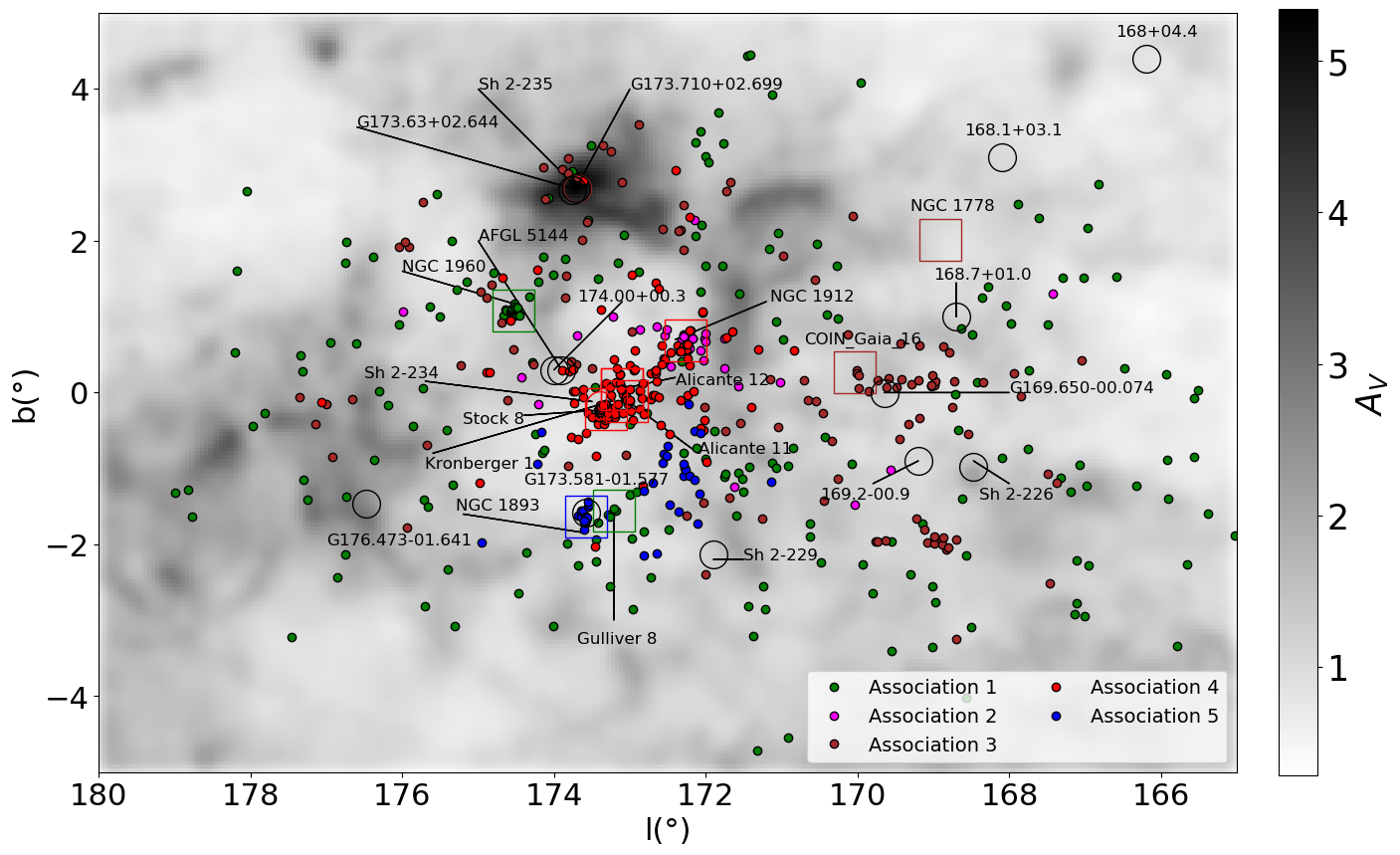
Figure 7: Spatial distribution in Galactic coordinates of the 5 new OB associations in Auriga. The background extinction map and the features highlighted in this map are the same as in Fig. 1.

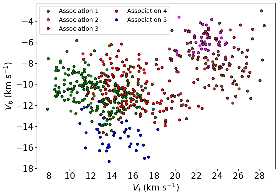
Figure 8: Transverse velocity distribution of the 5 new OB associations in Auriga.

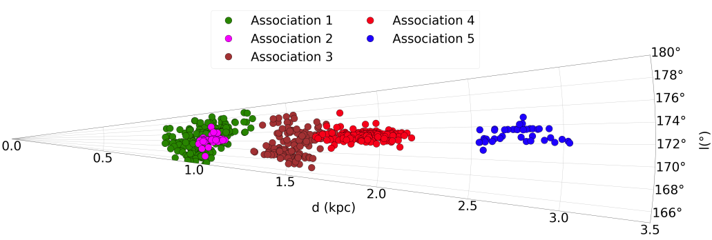
Figure 9: Galactic longitude as a function of SED-fitted distance for the 5 new OB associations in Auriga. The median error bars on distances are respectively $\sim$ 30 pc for associations 1 and 2, $\sim$ 50 pc for association 3, $\sim$ 70 pc for association 4 and $\sim$ 160 pc for association 5.

3.7 Comparison with historical associations and open clusters

We crossmatch the members of our new OB associations with the historical members of Aur OB1 and OB2 from Melnik & Dambis (2020) and the open cluster members from Cantat-Gaudin & Anders (2020), with the results displayed in Table 3.

Table 3: Comparison between our new OB association members and OB stars in the historical associations and in the open clusters from Cantat-Gaudin & Anders (2020). $N_{\rm hist}$ stands for the number of stars in a historical association whilst $N_{\rm OC}$ designates the number of stars in an open cluster. The notations CG16, G8, K1 and S8 stand respectively for COIN-Gaia_16, Gulliver 8, Kronberger 1 and Stock 8.

Assoc.	$N_{\rm hist}$	Hist. assoc.	$N_{\rm OC}$	OC
1	7	Aur OB1	25, 4	NGC 1960, G8
2			26	NGC 1912
3	1	Aur OB1	9, 4	NGC 1778, CG16
4	1, 8	Aur OB1, OB2	49, 5	S8, K1
5	2	Aur OB2	15	NGC 1893

Association 1 includes stars in both Aur OB1 and NGC 1960 and is the largest foreground association in the area. The other historical members of Aur OB1 are spread over the other new OB associations. Associations 4 and 5 have significant overlaps with Stock 8 and NGC 1893. This comparison suggests that NGC 1893 is located closer than previous estimations (Lim et al., 2018; Cantat-Gaudin & Anders, 2020) at a distance of $\sim$2.8 kpc, consistent with the distance from Mel’Nik & Dambis (2009).

4 Analysis of the new OB associations

In this section we perform a kinematic and physical analysis of the new OB associations in Auriga, studying their expansion and star formation history.

Table 4: Properties of the new OB associations. The first column indicates the parameter, where the subscript ’m’ indicates the median value and ’$\sigma$’ the dispersion. The total initial stellar mass is corrected for observational incompleteness, as described in the text.

Parameters	Units	Assoc. 1	Assoc. 2	Assoc. 3	Assoc. 4	Assoc. 5
${\rm RA(ICRS)}_{m}$	deg	81.30	82.13	80.16	82.02	80.70
${\rm DE(ICRS)}_{m}$	deg	34.97	35.84	36.57	34.77	33.94
$l_{m}$	deg	170.72	172.24	170.70	173.09	172.82
$b_{m}$	deg	-0.16	0.70	0.11	-0.03	-1.48
$d_{m}$	pc	1056	1085	1514	1923	2760
$\sigma_{d}$	pc	102.2	25.2	76.0	103.8	-
$V_{l_{m}}$	km s-1	12.98	22.85	23.69	15.37	14.18
$\sigma_{V_{l}}$	km s-1	2.52	1.09	2.96	2.20	2.10
$V_{b_{m}}$	km s-1	-10.75	-6.16	-8.10	-10.58	-14.84
$\sigma_{V_{b}}$	km s-1	1.41	0.95	2.00	2.05	1.17
Observed number of B stars		$194\pm 3$	$40^{+2}_{-1}$	$107^{+3}_{-2}$	$115^{+3}_{-4}$	$32\pm 2$
Observed number of O stars		$12^{+3}_{-2}$	$0\pm 0$	$4\pm 1$	$13\pm 2$	$3^{+2}_{-1}$
Total stellar initial mass	$M_{\odot}$	$6051^{+426}_{-387}$	$1219^{+182}_{-167}$	$3075^{+298}_{-276}$	$3500^{+315}_{-306}$	$879^{+163}_{-136}$
HR diagrams age	Myr	0-30	-	0-20	0-5	0-10
Related OCs age	Myr	18-26	250-375	26	4-8	1-5
Traceback age	Myr	$20.9^{+1.1}_{-1.2}$	$369.9^{+8.3}_{-22.2}$	$11.7^{+7.2}_{-3.0}$	$1.6^{+1.3}_{-0.9}$	-
Age	Myr	$\sim$ 20	-	10-20	0-5	0-10

4.1 Physical properties of the individual associations

We have estimated the observed number of O- and B-type stars in each association. To do so we defined B-type stars as those with SED-fitted $\log(T_{\rm eff})>4$ and $\log(T_{\rm eff})<4.3$ and O-type stars as those with SED-fitted $\log(T_{\rm eff})>4.3$, using the same thresholds than in Section 3.3. Uncertainties were estimated through a Monte Carlo experiment where the effective temperature of each star was randomly sampled within their uncertainties. This is shown in Table 4 and, in line with the HR diagrams in Fig. 10, shows a dominance of late B-type stars and a few O-type stars.

To determine the total mass of each association, we first identified the range of masses over which our sample completeness is expected to be unbiased by the age of our stars. We chose this mass range to be 2.5 $M_{\odot}$ (the mass of an A0 star) to 7.1 $M_{\odot}$ (the post main-sequence turn-off mass at an age of 50 Myr, Ekström et al. 2012). We then corrected the number of stars according to the incompleteness levels we have calculated and displayed in Fig. 5.

We performed a Monte Carlo simulation sampling stellar masses at random using the mass function from Maschberger (2013). We counted both the number of stars in our selected mass range and the total number and mass of stars. We stopped the simulation only when we reached the total number of observed stars in the selected mass range. This process was repeated 10,000 times, using the uncertainties on the individual SED-fitted stellar masses, to obtain an uncertainty for the total stellar mass of each association. These are provided in Table 4 and range from $\sim$900 to $\sim$6000 M_⊙. The most massive is association 1, with an estimated initial stellar mass of $\sim$6000 M_⊙ and currently containing about 200 B-type members.

4.2 Kinematic properties of the individual associations

We calculated the median coordinates (equatorial and galactic), distances and transverse velocities for each OB association. In addition, we have computed the intrinsic dispersion in distance and transverse velocities based on the method from Ivezić et al. (2014) using the observational uncertainties. The distance dispersions typically range up to a few tens of pc, while the velocity dispersions range up to 3 km s^-1, consistent with that of other OB associations (Wright, 2020).

4.3 HR diagrams of association members

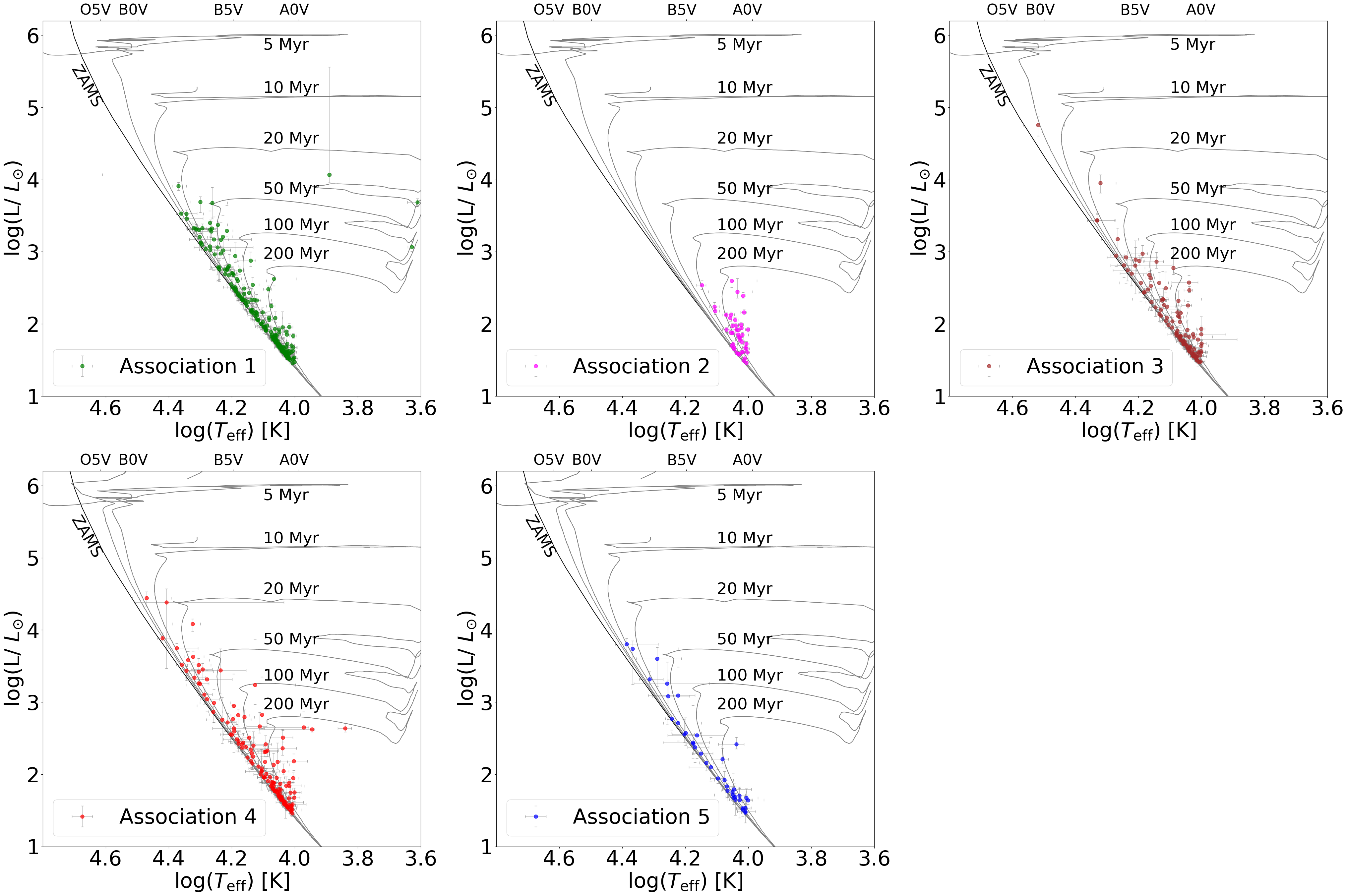
Figure 10: HR diagrams for the members of the new OB associations in Auriga. Isochrones have been shown from the rotating evolutionary models from Ekström et al. (2012). Positions of some spectral types have been indicated on the top horizontal axis for clarity.

Fig. 10 shows the HR diagrams for each association, produced with the SED-fitted effective temperatures and luminosities. It is clear that the identified members are dominated by late B-type stars, preventing a straightforward age assessment. Association 1 contain a few stars close to the 50, 100 and 200 Myr isochrones, which would make this much older than other known OB associations, though these may be contaminants. Associations 3 to 5 contain hotter stars that suggest a younger age of $<$ 20 Myr.

There are a number of factors that can affect the positions of stars in the HR diagram. First among these is extinction, which is derived for each star individually as part of our SED fitting process from the extinction map. The uncertainty in the extinction to a given star, which is derived from the distance uncertainty, propagates through to the uncertainty on the effective temperature and luminosity shown in the HR diagram. An alternative approach might be to use a single extinction value for all members of an association, but the effect of this will be small as the variation in extinction across members of an association is small, with a typical standard deviation in $A_{V}$ of 0.2 - 0.6 mag. Such a difference in reddening does have a small effect on the derived physical parameters. However, if we reproduce these HR diagrams using the median extinction for all association members, while there are small changes in the position of each star, the extreme outliers do not change significantly.

More significant factors affecting the position of stars in the HR diagram include binarity, and the presence of possible contaminants. Association 1 constitutes a good example of this, for which most of its stars are close to the ZAMS and therefore consistent with being under 20 Myr old, suggesting that its stars sitting on the 50, 100 and 200 Myr isochrones may be contaminants.

4.4 Expansion and traceback age

Fig. 10 shows that many of the OB associations in Auriga have ages of several tens of Myr. Therefore, instead of using a linear expansion model to determine their expansion age, we trace back the associations using the epicycle approximation from Fuchs et al. (2006), and correct for the local standard of rest (LSR) from the values of Schönrich et al. (2010). We gather RVs from the APOGEE survey and from SIMBAD. RVs from the literature are discarded if they lack an uncertainty or if their measurement is considered unreliable. If some stars belong to both APOGEE and SIMBAD, we take the weighted mean of the two values. In doing so we obtain a sample of 95 stars with RVs.

We calculated the median RV for each association and track back whole associations rather than individual stars, due to the effects of unresolved close binaries. Again we apply a Monte Carlo’s simulation to compute the uncertainties on the median velocities following the method in Quintana & Wright (2022). The results are shown in Table 5.

Table 5: RVs calculated for the new OB associations. $N_{RV}$ is the number of stars with a reliable measured RV. References are: (1): APOGEE, (2): Fehrenbach et al. (1992), (3): Grenier et al. (1999), (4): Gontcharov (2006), (5): Turner et al. (2011), (6): Chojnowski et al. (2017), (7): Gaia Collaboration et al. (2018), (8): Zhong et al. (2020)

Assoc.	$N_{RV}$	RV (km s-1)	References
1	47	$2.13\pm 1.26$	All but (6)
2	5	$6.59\pm 4.31$	(8)
3	8	$-4.64\pm 3.01$	(1), (6), (8)
4	31	$4.12\pm 1.63$	(1), (7), (8)
5	4	$1.46\pm 7.45$	(8)

Combining RVs with Gaia PMs allows us to perform a 3D traceback on these associations. We use the HR diagrams (Fig. 10) together with the ages of the related open clusters to add constraints on the age estimations, which are displayed in Table 1. With this information, we set the upper limit on traceback to 50 Myr in the past for associations 1 and 5, 400 Myr for association 2, 30 Myr for association 3 and 20 Myr for association 4. We trace back each association in time steps of 0.1 Myr, and at each time step we calculate the MAD (median absolute deviation) in Galactic coordinates of the on-sky spatial distribution of association members, and we estimate the time of minimum MAD when the association is at its most compact. We repeat this process 1000 times to derive uncertainties. An example is shown in Fig. 11 for association 1, while the other associations are shown in Figure 13.

We estimated ages for each association based on the combination of (i) the time for the system to trace back to its most compact state, (ii) the age of any open cluster or star-forming region linked to the association (Section 3.7), and (iii) any age constraints arising from the HR diagram (Fig. 10). These ages are listed in Table 4. For some systems the traceback was able to place reasonable constraints on the age of the system, (e.g., for association 1), while for other associations the best constraint came from the open clusters and star-forming regions the association was linked to (e.g., for associations 4 and 5). For the remaining associations either the HR diagram provided the best constraint on the age (e.g., for association 3) or very little constraint was possible by any means (e.g., association 2).

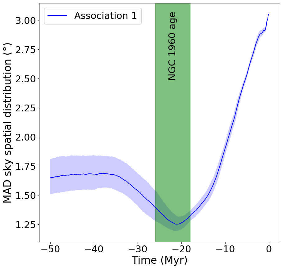
Figure 11: MAD of the on-sky spatial distribution for members of association 1 as a function of traceback time. The age of the related open cluster (NGC 1960) is shown, taken from Table 1.

5 Discussion

In this section we discuss our findings and how the new Auriga OB associations can help understand the star formation history of the region. Our main results are outlined as follows:

• We have shown that both Aur OB1 and Aur OB2 are too extended in PM and distance to be genuine OB associations, encouraging us to revisit the census of OB stars and associations in the region.

• We identified more than 5000 candidate OB stars across the region using our SED fitter, with an estimated reliability of 90 %.

• We identified 5 new high-confidence OB associations in the area that we analysed physically and kinematically, and estimated their age through a combination of 3D kinematic traceback, their link to open clusters and star-forming regions with known ages, and the distribution of members in the HR diagram. Only a small fraction ($\sim$10 %) of the identified OB stars have been assigned to these associations.

5.1 The new Auriga OB associations

We have identified 5 new OB associations in Auriga, with total stellar masses from a few hundreds to a few thousand solar masses, and with kinematic properties consistent with other OB associations (Wright, 2020). They are likely related to open clusters in the area (see Table 3).

Association 1 shares several members with Aur OB1 and is related to NGC 1960, so it should be seen as the replacement for the historical Aur OB1 association. Similarly, the historical members of Aur OB2 are now divided between associations 4 and 5, respectively related to Stock 8 and NGC 1893. This confirms the suggestion of Marco & Negueruela (2016) to divide Aur OB2 into two different associations, one in the foreground and one in the background.

The Hii region Sh 2-235 instead appears to be related to association 3, since it is located at a similar distance of $1.36\pm 0.27$ kpc (Foster & Brunt, 2015). Association 3 also includes HD 36483, an O9.5IV star (Sota et al., 2011), which may be responsible for ionizing the Hii region.

Association 4 occupies the centre of our region of study, where three OCs are found, along with the Hii region Sh 2-234 (Fig. 7). Sh 2-234 is located at a distance of $2.19\pm 0.10$ kpc (Foster & Brunt, 2015). Its relation to Aur OB2 and the surrounding OCs has been suggested by Marco & Negueruela (2016) and we confirm it to be related to association 4. We cannot comment on whether the star LS V +34 23 is part of association 4 (previously in Aur OB2 and thought to be responsible for ionizing Sh 2-234, Marco & Negueruela 2016) as its Gaia photometry failed our quality checks, preventing us from performing an SED fit. However, association 4 does contain LS V + 34 15, LS V + 34 21 and LS V + 35 25, of respective spectral types O5.5V (Negueruela et al., 2007), O9IV (Roman-Lopes & Roman-Lopes, 2019) and O9.5V (Georgelin et al., 1973), each probable sources of ionization for the Hii region Sh 2-234. However, the RV of Sh 2-234 has been measured as $-21.4\pm 0.2$ km s^-1 (Anderson et al., 2015), which is significantly different from the RV we estimated for association 4 (Table 5), even if those stars are responsible for ionizing the Hii region, the association and the Hii region may not otherwise be related.

5.2 Expansion and age of the OB associations

Our analysis revealed that our OB associations have various ages, from the youngest associations 4 and 5 with ages $<$ 10 Myr to associations of several tens of Myr old (association 3). For the OB associations where multiple age indicators were available, the ages derived by different methods were consistent. The exception to this is association 2, with the majority of its OB stars consistent with being on the ZAMS (Fig. 10) while its related OC is several hundreds of Myr old (Table 1), far older than most OB associations.

In Section 4.4 we showed that nearly all our OB associations traced back into a more compact configuration in the past, which is a signature of expansion (see e.g. Wright & Mamajek 2018 and Miret-Roig et al. 2022). We however point out that associations 4 and 5 reached their most compact state very recently (Fig. 13).

5.3 OB stars unassigned to groups

The 5 OB associations contain 554 OB stars in total from our sample of 5617 SED-fitted OB stars in the area. This means that $\sim$90 % of the OB stars have been unassigned to any stellar group, which could be explained by several factors.

In Section 3.6, we imposed a minimum size of 15 OB stars per association to be consistent with their definition (Humphreys, 1978; Wright, 2020). There could be other stellar groups in the area which are dominated by low-mass stars and only contain a handful of OB stars. Similarly, some OB stars initially belonging to a group were rejected during the bootstrapping process (see Table 2). This was particularly the case for most distant stars ($>2$ kpc) as the Gaia parallaxes become less precise.

Our sample includes many late B-type stars. A B9 star with an initial stellar mass of 2.75 $M_{\odot}$ (Pecaut & Mamajek, 2013) has a lifetime of $\sim$ 700 Myr as predicted by stellar evolutionary models (Ekström et al., 2012). This value is far beyond the typical lifetime of an OB association (Wright, 2020) and implies that even if those stars were born clustered, they would probably have dispersed into the Galactic field population since.

It is also possible that some of these OB stars formed within associations but were ejected and became runaways. Notably, massive stars are more likely to belong to multiple systems (Lada, 2006), and when the primary star undergoes a supernova explosion, it can eject the secondary star beyond the group it was born into.

5.4 Distribution of OB associations and Galactic structure

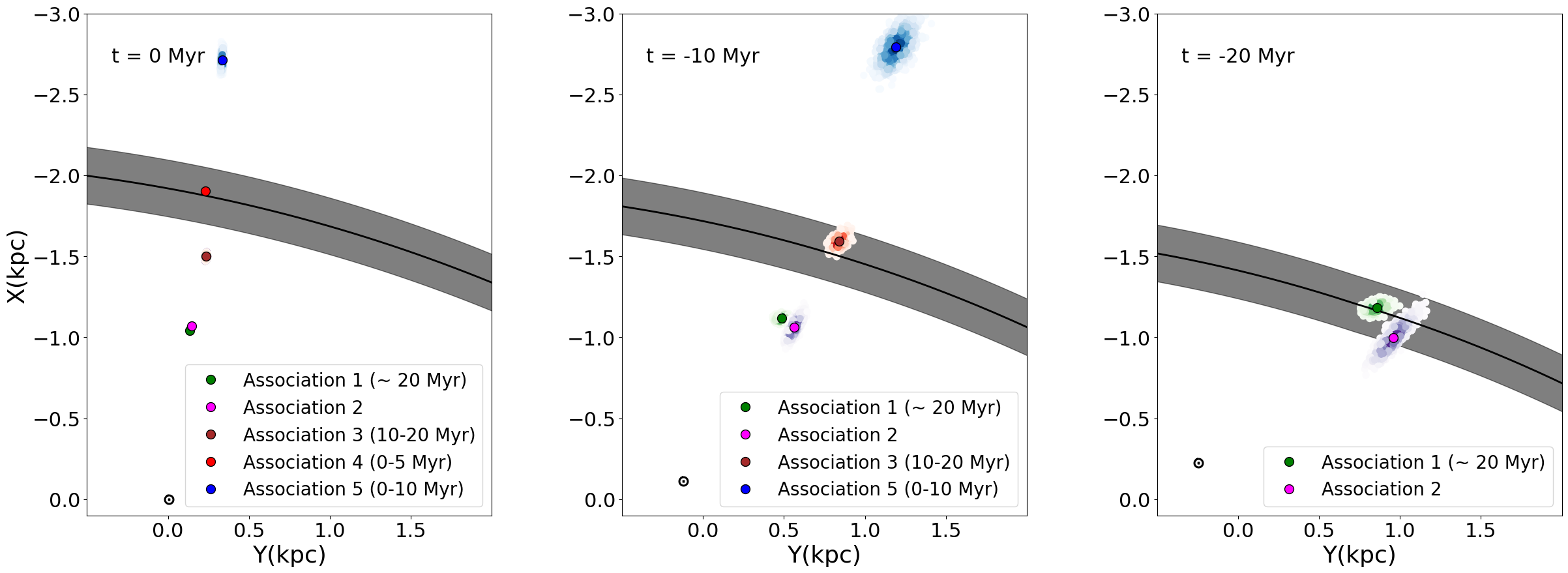
Figure 12: Median positions of the OB associations across the X-Y plane from the present time to 20 Myr in the past, shown relative to the Local Standard of Rest. Uncertainties on their position from the traceback have been shown as a blur. The Perseus spiral arm model, including its thickness, is from Reid et al. (2019). The Sun symbol corresponds to the position of the Sun.

The Perseus spiral arm intercepts our sightline at a distance of approximately 2 kpc (Reid et al., 2019), at approximately the position of association 4, the youngest of our new OB associations. Fig. 12 shows the positions of our new OB associations, with their ages, relative to the position of the Perseus spiral arm. While association 4 is coincident with the current position of the Perseus spiral arm, the associations closer to us are older, indicating a potential age gradient.

To determine whether this age gradient is related to the motion of the Perseus spiral arm, we model the positions of the spiral arm and our new OB associations over the last 20 Myrs. We use the spiral arm model from Reid et al. (2019) and the spiral arm pattern speed of $\Omega_{p}=-28.2\pm 2.1$ km s^-1 from Dias et al. (2019). We trace back the position of the Perseus spiral arm 20 Myr into the past in the frame of the LSR.

Fig. 12 shows the position of the OB associations with the Perseus spiral arms, at intervals of 10 Myr, back to 20 Myr in the past. At 10 Myr in the past it is clear that association 3 (with an estimated age of 10-20 Myr) is coincident with the spiral arm, while at 20 Myr in the past, association 1 (estimated age of $\sim$20 Myr) is coincident with the spiral arm. Association 2 crosses the spiral arm $\sim$20 Myr ago as well, despite its related OC and traceback suggesting an older age (Fig. 13), which may suggest that the association is younger and not related to NGC 1912, or that the association did not form within the spiral arm. As for association 5, it stays too distant to be related to the Perseus spiral arm and may have formed outside (or in the Outer spiral arm).

This result shows that OB associations can be used not only as tracers for the current positions of spiral arms but also as a probe for the star formation history of a region and potentially the progress of a spiral arm through the region.

6 Conclusions

We have shown that Aur OB1 and OB2 are not genuine OB associations, because their members are characterized by a too large spread in proper motion and distance. Applying an improved SED fitting tool, we have identified 5617 OB stars with a reliability of $\sim$ 90 % for the lowest temperature threshold.

Using a clustering algorithm (HDBSCAN), we have identified 5 high-confidence OB associations that we connect to the open clusters and star-forming regions in the area. Association 1 is the main foreground association at a distance of $\sim$ 1 kpc and with a mass of $\sim$ 6000 $M_{\odot}$ and should replace Aur OB1 due to its common members and relation with NGC 1960. Similarly, we argue that Aur OB2 should be replaced by association 4 (at $\sim$ 1.9 kpc and with a total mass of $\sim$ 3500 $M_{\odot}$), and 5 (at $\sim$ 2.8 kpc and with a total mass of $\sim$ 900 $M_{\odot}$).

We have analysed these OB associations, combining HR diagrams and kinematic traceback, to constrain their ages. We have also studied their expansion, their total stellar masses, their number of OB stars and their 3D position.

We have also identified an age progression between several of these associations, that suggests their origins may have been within the Perseus spiral arm. This shows that OB associations constitute useful tools to study recent star formation history and the position and motion of the Galactic spiral arms.

Data Availability

The data underlying this article will be uploaded to Vizier.

Appendix A Traceback diagrams

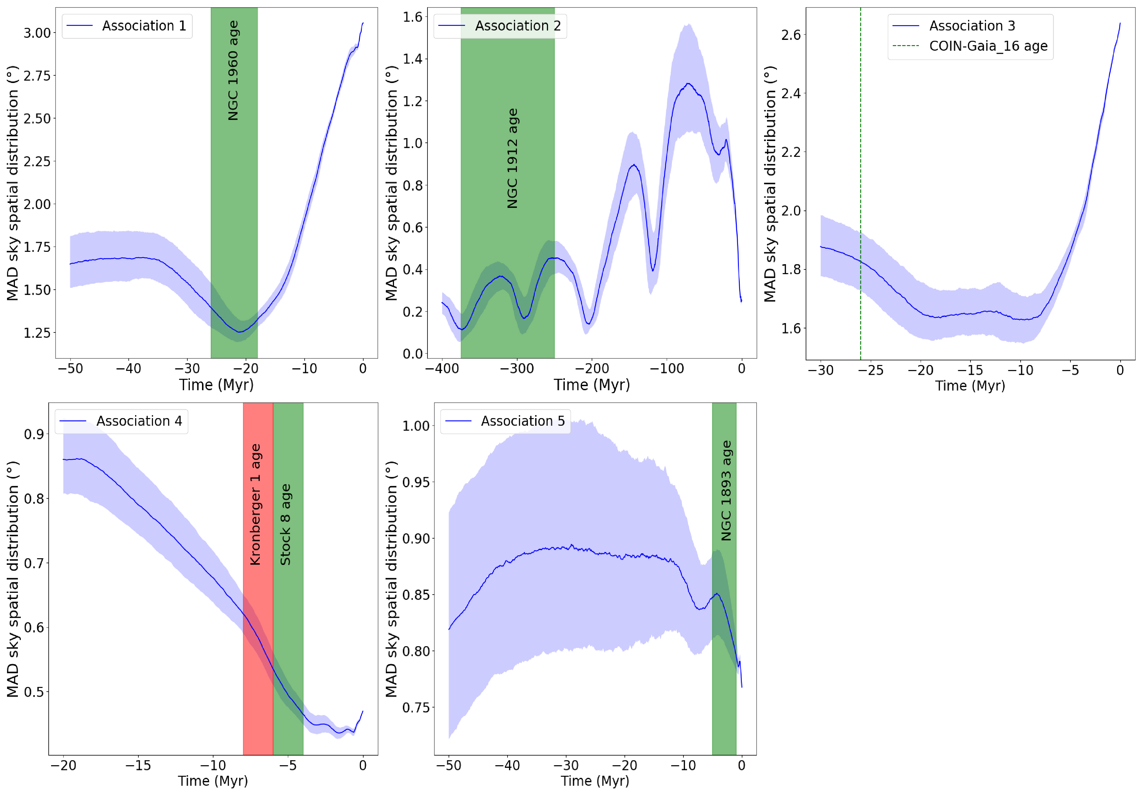
Figure 13: MAD of the on-sky distribution of members of each association as a function of traceback time.

References

- Abdurro’uf et al. (2022) Abdurro’uf et al., 2022, ApJS, 259, 35
- Ambartsumian (1947) Ambartsumian V. A., 1947, The evolution of stars and astrophysics. Armenian SSR Academy of Sciences Press
- Anderson et al. (2015) Anderson L. D., Armentrout W. P., Johnstone B. M., Bania T. M., Balser D. S., Wenger T. V., Cunningham V., 2015, ApJS, 221, 26
- Armstrong et al. (2020) Armstrong J. J., Wright N. J., Jeffries R. D., Jackson R. J., 2020, MNRAS, 494, 4794
- Astropy Collaboration et al. (2013) Astropy Collaboration et al., 2013, A&A, 558, A33
- Bailer-Jones (2015) Bailer-Jones C. A. L., 2015, PASP, 127, 994
- Bailer-Jones et al. (2021) Bailer-Jones C. A. L., Rybizki J., Fouesneau M., Demleitner M., Andrae R., 2021, AJ, 161, 147
- Barbon & Hassan (1973) Barbon R., Hassan S. M., 1973, A&AS, 10, 1
- Barentsen et al. (2014) Barentsen G., et al., 2014, MNRAS, 444, 3230
- Blaauw (1964) Blaauw A., 1964, ARA&A, 2, 213
- Bok (1934) Bok B. J., 1934, Harvard College Observatory Circular, 384, 1
- Cantat-Gaudin & Anders (2020) Cantat-Gaudin T., Anders F., 2020, A&A, 633, A99
- Cantat-Gaudin et al. (2019) Cantat-Gaudin T., et al., 2019, A&A, 626, A17
- Cantat-Gaudin et al. (2020) Cantat-Gaudin T., et al., 2020, A&A, 640, A1
- Casey (2016) Casey A. R., 2016, ApJS, 223, 8
- Chojnowski et al. (2017) Chojnowski S. D., et al., 2017, AJ, 153, 174
- Coelho (2014) Coelho P. R. T., 2014, MNRAS, 440, 1027
- Creevey et al. (2022) Creevey O. L., et al., 2022, arXiv e-prints, p. arXiv:2206.05864
- Cutri et al. (2003) Cutri R. M., et al., 2003, 2MASS All Sky Catalog of point sources.. NASA/IPAC Infrared Science Archive
- Delchambre et al. (2022) Delchambre L., et al., 2022, arXiv e-prints, p. arXiv:2206.06710
- Dias et al. (2019) Dias W. S., Monteiro H., Lépine J. R. D., Barros D. A., 2019, MNRAS, 486, 5726
- Dias et al. (2021) Dias W. S., Monteiro H., Moitinho A., Lépine J. R. D., Carraro G., Paunzen E., Alessi B., Villela L., 2021, MNRAS, 504, 356
- Dib et al. (2018) Dib S., Schmeja S., Parker R. J., 2018, MNRAS, 473, 849
- Drew et al. (2005) Drew J. E., et al., 2005, MNRAS, 362, 753
- Drew et al. (2014) Drew J. E., et al., 2014, MNRAS, 440, 2036
- Ekström et al. (2012) Ekström S., et al., 2012, A&A, 537, A146
- El-Badry et al. (2021) El-Badry K., Rix H.-W., Heintz T. M., 2021, MNRAS, 506, 2269
- Fehrenbach et al. (1992) Fehrenbach C., Burnage R., Figuiere J., 1992, A&AS, 95, 541
- Fitzpatrick et al. (2019) Fitzpatrick E. L., Massa D., Gordon K. D., Bohlin R., Clayton G. C., 2019, ApJ, 886, 108
- Foreman-Mackey et al. (2013) Foreman-Mackey D., Hogg D. W., Lang D., Goodman J., 2013, PASP, 125, 306
- Foster & Brunt (2015) Foster T., Brunt C. M., 2015, AJ, 150, 147
- Fuchs et al. (2006) Fuchs B., Breitschwerdt D., de Avillez M. A., Dettbarn C., Flynn C., 2006, MNRAS, 373, 993
- Gaia Collaboration et al. (2018) Gaia Collaboration et al., 2018, A&A, 616, A1
- Gaia Collaboration et al. (2021) Gaia Collaboration et al., 2021, A&A, 649, A1
- García Pérez et al. (2016) García Pérez A. E., et al., 2016, AJ, 151, 144
- Georgelin et al. (1973) Georgelin Y. M., Georgelin Y. P., Roux S., 1973, A&A, 25, 337
- Gontcharov (2006) Gontcharov G. A., 2006, Astronomy Letters, 32, 759
- Green et al. (2019) Green G. M., Schlafly E., Zucker C., Speagle J. S., Finkbeiner D., 2019, ApJ, 887, 93
- Grenier et al. (1999) Grenier S., et al., 1999, A&AS, 137, 451
- Gyulbudaghian (2011) Gyulbudaghian A. L., 2011, Astrophysics, 54, 476
- Hills (1980) Hills J. G., 1980, ApJ, 235, 986
- Hodgkin et al. (2009) Hodgkin S. T., Irwin M. J., Hewett P. C., Warren S. J., 2009, MNRAS, 394, 675
- Humphreys (1978) Humphreys R. M., 1978, ApJS, 38, 309
- Humphreys & McElroy (1984) Humphreys R. M., McElroy D. B., 1984, ApJ, 284, 565
- Ivezić et al. (2014) Ivezić Ž., Connelly A. J., Vand erPlas J. T., Gray A., 2014, Statistics, Data Mining, and Machine Learning in Astronomy
- Jacobson et al. (2002) Jacobson H. R., Cummings J., Deliyannis C. P., Steinhauer A., Sarajedini A., 2002, in American Astronomical Society Meeting Abstracts. p. 124.07
- Jeffries et al. (2013) Jeffries R. D., Naylor T., Mayne N. J., Bell C. P. M., Littlefair S. P., 2013, MNRAS, 434, 2438
- Jose et al. (2008) Jose J., et al., 2008, MNRAS, 384, 1675
- Joshi et al. (2020) Joshi Y. C., Maurya J., John A. A., Panchal A., Joshi S., Kumar B., 2020, MNRAS, 492, 3602
- Kerr et al. (2021) Kerr R. M. P., Rizzuto A. C., Kraus A. L., Offner S. S. R., 2021, ApJ, 917, 23
- Kharchenko et al. (2005) Kharchenko N. V., Piskunov A. E., Röser S., Schilbach E., Scholz R. D., 2005, A&A, 438, 1163
- Kharchenko et al. (2013) Kharchenko N. V., Piskunov A. E., Schilbach E., Röser S., Scholz R. D., 2013, A&A, 558, A53
- Kounkel et al. (2018) Kounkel M., et al., 2018, AJ, 156, 84
- Kroupa et al. (2001) Kroupa P., Aarseth S., Hurley J., 2001, MNRAS, 321, 699
- Kruijssen (2012) Kruijssen J. M. D., 2012, MNRAS, 426, 3008
- Kuhn et al. (2019) Kuhn M. A., Hillenbrand L. A., Sills A., Feigelson E. D., Getman K. V., 2019, ApJ, 870, 32
- Lada (2006) Lada C. J., 2006, ApJ, 640, L63
- Lada & Lada (2003) Lada C. J., Lada E. A., 2003, ARA&A, 41, 57
- Lim et al. (2014) Lim B., Sung H., Kim J. S., Bessell M. S., Park B.-G., 2014, MNRAS, 443, 454
- Lim et al. (2018) Lim B., et al., 2018, MNRAS, 477, 1993
- Lindegren et al. (2021a) Lindegren L., et al., 2021a, A&A, 649, A2
- Lindegren et al. (2021b) Lindegren L., et al., 2021b, A&A, 649, A4
- Lucas et al. (2008) Lucas P. W., et al., 2008, MNRAS, 391, 136
- Marco & Negueruela (2016) Marco A., Negueruela I., 2016, MNRAS, 459, 880
- Marco et al. (2001) Marco A., Bernabeu G., Negueruela I., 2001, AJ, 121, 2075
- Martins et al. (2005) Martins F., Schaerer D., Hillier D. J., 2005, A&A, 436, 1049
- Maschberger (2013) Maschberger T., 2013, MNRAS, 429, 1725
- McInnes et al. (2017) McInnes L., Healy J., Astels S., 2017, The Journal of Open Source Software, 2, 205
- Mel’Nik & Dambis (2009) Mel’Nik A. M., Dambis A. K., 2009, MNRAS, 400, 518
- Mellinger (2008) Mellinger A., 2008, in Reipurth B., ed., , Vol. 4, Handbook of Star Forming Regions, Volume I. p. 1
- Melnik & Dambis (2020) Melnik A. M., Dambis A. K., 2020, MNRAS, 493, 2339
- Miret-Roig et al. (2022) Miret-Roig N., Galli P. A. B., Olivares J., Bouy H., Alves J., Barrado D., 2022, A&A, 667, A163
- Monguió et al. (2020) Monguió M., et al., 2020, A&A, 638, A18
- Morgan et al. (1953) Morgan W. W., Whitford A. E., Code A. D., 1953, ApJ, 118, 318
- Negueruela & Marco (2003) Negueruela I., Marco A., 2003, A&A, 406, 119
- Negueruela et al. (2007) Negueruela I., Marco A., Israel G. L., Bernabeu G., 2007, A&A, 471, 485
- Paladini et al. (2003) Paladini R., Burigana C., Davies R. D., Maino D., Bersanelli M., Cappellini B., Platania P., Smoot G., 2003, A&A, 397, 213
- Pandey et al. (2007) Pandey A. K., Sharma S., Upadhyay K., Ogura K., Sandhu T. S., Mito H., Sagar R., 2007, PASJ, 59, 547
- Pandey et al. (2020) Pandey A. K., Sharma S., Kobayashi N., Sarugaku Y., Ogura K., 2020, MNRAS, 492, 2446
- Panja et al. (2021) Panja A., Chen W. P., Dutta S., Sun Y., Gao Y., Mondal S., 2021, ApJ, 910, 80
- Pecaut & Mamajek (2013) Pecaut M. J., Mamajek E. E., 2013, ApJS, 208, 9
- Quintana & Wright (2021) Quintana A. L., Wright N. J., 2021, MNRAS, 508, 2370
- Quintana & Wright (2022) Quintana A. L., Wright N. J., 2022, MNRAS, 515, 687
- Rauch & Deetjen (2003) Rauch T., Deetjen J. L., 2003, Handling of Atomic Data. Stellar Atmosphere Modeling, ASP Conference Proceedings, Vol. 288. in Tuebingen, Germany. Editors: Ivan Hubeny, Dimitri Mihalas, and Klaus Werner. San Francisco: Astronomical Society of the Pacific, p. 103
- Reid et al. (2019) Reid M. J., et al., 2019, ApJ, 885, 131
- Riello et al. (2021) Riello M., et al., 2021, A&A, 649, A3
- Roberts (1972) Roberts William W. J., 1972, ApJ, 173, 259
- Roman-Lopes & Roman-Lopes (2019) Roman-Lopes A., Roman-Lopes G. F., 2019, MNRAS, 484, 5578
- Santos-Silva et al. (2021) Santos-Silva T., et al., 2021, MNRAS, 508, 1033
- Schönrich et al. (2010) Schönrich R., Binney J., Dehnen W., 2010, MNRAS, 403, 1829
- Sharma et al. (2007) Sharma S., Pandey A. K., Ojha D. K., Chen W. P., Ghosh S. K., Bhatt B. C., Maheswar G., Sagar R., 2007, MNRAS, 380, 1141
- Skrutskie et al. (2006) Skrutskie M. F., et al., 2006, AJ, 131, 1163
- Sota et al. (2011) Sota A., Maíz Apellániz J., Walborn N. R., Alfaro E. J., Barbá R. H., Morrell N. I., Gamen R. C., Arias J. I., 2011, ApJS, 193, 24
- Straižys et al. (2010) Straižys V., Drew J. E., Laugalys V., 2010, Baltic Astronomy, 19, 169
- Subramaniam & Sagar (1999) Subramaniam A., Sagar R., 1999, AJ, 117, 937
- Tapia et al. (1991) Tapia M., Costero R., Echevarria J., Roth M., 1991, MNRAS, 253, 649
- Taylor (2005) Taylor M. B., 2005, in Shopbell P., Britton M., Ebert R., eds, Astronomical Society of the Pacific Conference Series Vol. 347, Astronomical Data Analysis Software and Systems XIV. p. 29
- Trundle et al. (2007) Trundle C., Dufton P. L., Hunter I., Evans C. J., Lennon D. J., Smartt S. J., Ryans R. S. I., 2007, A&A, 471, 625
- Turner et al. (2011) Turner D. G., Rosvick J. M., Balam D. D., Henden A. A., Majaess D. J., Lane D. J., 2011, PASP, 123, 1249
- Ward & Kruijssen (2018) Ward J. L., Kruijssen J. M. D., 2018, MNRAS, 475, 5659
- Werner & Dreizler (1999) Werner K., Dreizler S., 1999, Journal of Computational and Applied Mathematics, 109, 65
- Werner et al. (2003) Werner K., Deetjen J. L., Dreizler S., Nagel T., Rauch T., Schuh S. L., 2003, Model Photospheres with Accelerated Lambda Iteration. Stellar Atmosphere Modeling, ASP Conference Proceedings, Vol. 288. Editors: Ivan Hubeny, Dimitri Mihalas, and Klaus Werner. San Francisco: Astronomical Society of the Pacific, p. 31
- Wright (2020) Wright N. J., 2020, New Astron. Rev., 90, 101549
- Wright & Mamajek (2018) Wright N. J., Mamajek E. E., 2018, MNRAS, 476, 381
- Wright et al. (2016) Wright N. J., Bouy H., Drew J. E., Sarro L. M., Bertin E., Cuillandre J.-C., Barrado D., 2016, MNRAS, 460, 2593
- Wright et al. (2022) Wright N. J., Goodwin S., Jeffries R. D., Kounkel M., Zari E., 2022, arXiv e-prints, p. arXiv:2203.10007
- Zari et al. (2021) Zari E., Rix H. W., Frankel N., Xiang M., Poggio E., Drimmel R., Tkachenko A., 2021, A&A, 650, A112
- Zhong et al. (2020) Zhong J., Chen L., Wu D., Li L., Bai L., Hou J., 2020, A&A, 640, A127