On approximating the temporal betweenness centrality through sampling

Abstract

We present a collection of sampling-based algorithms for approximating the temporal betweenness centrality of all nodes in a temporal graph. Our methods can compute probabilistically guaranteed high-quality temporal betweenness estimates (of nodes and temporal edges) under all the feasible temporal path optimalities presented in the work of Buß et al. (KDD, 2020). We provide a sample-complexity analysis of these methods and we speed up the temporal betweenness computation using progressive sampling techniques. Finally, we conduct an extensive experimental evaluation on real-world networks and we compare their performances in approximating the betweenness scores and rankings.

Keywords betweenness  $\cdot$ temporal graphs  $\cdot$ graph mining

1 Introduction

Computing the betweenness centrality is arguably one of the most important tasks in graph mining and network analysis. It finds application in several fields including social network analysis [1, 2], routing [3], machine learning [4], and neuroscience [5]. The betweenness of a node in a graph indicates how often this node is visited by a shortest path. High betweenness nodes are usually considered to be important in the network. Brandes’ algorithm [6], is the best algorithm to compute the exact centrality scores of every node in $\mathcal{O}(|V|\cdot|E|)$ time and $\mathcal{O}(|V|+|E|)$ space. Unfortunately, this algorithm quickly becomes impractical on nowadays networks with billion of nodes and edges. Moreover, there is theoretical evidence, in form of several conditional lower bounds results [7, 8], for believing that a faster algorithm cannot exists, even for approximately computing the betweenness. A further challenge, is that modern real-world networks are also dynamic or temporal i.e., they change over time. These challenges make essential to consider temporal variants of the betweenness centrality alongside algorithms with an excellent scaling behavior. Buß et al. [9, 10] gave several definitions of the temporal betweenness as a temporal counterpart of the betweenness centrality, characterized their computational complexity, and provided polynomial time algorithms to compute these temporal centrality measures. However, these algorithms turn out to be impractical, even for medium size networks. Thus, it is reasonable to consider approximation algorithms that can efficiently compute the centrality values of the nodes up to some small error. In this work, we follow the approach of Santoro et al. [11], and we provide a set of approximation algorithms for all the betweenness variants in [9].

Contributions.

We provide a suite of sampling-based algorithms for approximating the temporal betweenness of all vertices in large temporal graphs. We start our study in Section 4 with an analysis of the sample size needed to achieve a good approximation by a sampling-based approach. Next, we define a randomized version of the exact algorithms in [9] and we provide a progressive sampling heuristic to speed up its overall running time. We proceed by extending the approach of Santoro et al. [11] to all the temporal betweenness notions that can be computed in polynomial time [9], and by proposing a progressive sampling version of such algorithm that uses bounds on Rademacher Averages as a stopping criterion. Additionally, we propose the temporal analogous of [12] i.e., another sampling-based approach to approximate the temporal betweenness. Where its static counterpart is used by the state-of-the-art approach to estimate the betweenness centrality [13]. We then define its progressive sampling version. In Section 5 we compare these algorithms in terms of their efficiency and quality of approximation.

2 Related Work

The literature on betweenness centrality being vast, we restrict our attention to approaches that are closest to ours. Thus, we focus on sampling-based approaches for the betweenness on static and temporal graphs.

Static betweenness.

Several approximation algorithms for the static betweenness computation have been proposed. The most effective and fastest algorithms use random sampling techniques [14, 15, 12, 16, 13, 17, 18]. These algorithms differ from each other for the sampling strategy and their probabilistic guarantees. In their early work, Riondato and Kornaropoulos [12], showed that it is possible to derive a sharper bound on the sample size by considering the vertex diameter of the graph instead of the size of the vertex set. Subsequently, Riondato and Upfal [16] improved this bound by considering the size of the largest weakly connected component, and proposed the first progressive sampling algorithm for approximating the betweenness of every node in a graph. Following this line of research, Borassi and Natale [13] defined what is considered to be the state-of-the-art algorithm for the betweenness centrality estimation. Their approach is a progressive version of the one in [12] that uses a fast heuristic to speed-up the shortest paths computation. Next, Cousins et al. [17] defined a unifying sampling framework for the estimators in [6, 12, 16]. Building on this, Pellegrina and Vandin [18] extended the shortest path computation heuristic in [13] to the approach of Riondato and Upfal in [16] and showed that their novel method requires a smaller samples size compared to the one needed by the state-of-the-art algorithm [13].

Temporal betweenness.

Tsalouchidou et al. [19], extended the well-known Brandes algorithm [6] to allow for distributed computation of betweenness in temporal graphs. Specifically, they studied shortest-fastest paths, considering the bi-objective of shortest length and shortest duration. Buß et al. [9] analysed the temporal betweenness centrality considering several temporal path optimality criteria, such as shortest (foremost), foremost, fastest, and prefix-foremost, along with their computational complexities. They showed that, when considering paths with increasing time labels, the foremost and fastest temporal betweenness variants are $\#P$-hard, while the shortest and shortest foremost ones can be computed in $O(|V|^{3}\cdot|T|^{2})$, and the prefix-foremost one in $O(|V|\cdot|\mathcal{E}|\cdot\log|\mathcal{E}|)$. Here $\mathcal{E}$ is the set of temporal edges, and $T$ is the set of unique time stamps. The complexity analysis of these measures has been further refined since [10]. Santoro et al. [11], provided the first sampling-based approximation algorithm for one variant of the temporal betweenness centrality. They gave theoretical results on the approximation guarantee of their framework leveraging on the empirical Bernstein bound, an advanced concentration inequality that (to the best of our knowledge) does not provide useful information about the sample size needed to achieve a given approximation error, nor can it be used to define a fast progressive sampling procedure that keeps sampling until the desired approximation is achieved.

3 Preliminaries

We proceed by formally introducing the terminology and concepts that we use in what follows. For $k\in\mathbb{N}$, we let $[k]=\{1,\dots k\}$.

3.0.1 Temporal Graphs and Paths.

We start by introducing temporal graphs. A directed temporal graph is an ordered tuple $\mathcal{G}=(V,\mathcal{E})$ where $\mathcal{E}=\{(u,v,t):u,v,\in V\land t\in[T]\}$ is the set of temporal edges. Undirected temporal graphs can be modeled via directed graphs resulting in a bi-directed temporal edges. Additionally, we define $V\times[T]$ as the set of vertex appearances. Given two nodes $s$ and $z$, a temporal path $tp_{sz}$ is a (unique) sequence of time-respecting temporal edges that starts from $s$ and ends in $z$, formally:

Definition 1 (Temporal Path)

Given a temporal graph $\mathcal{G}$, a temporal path $tp$ from $s\in V$ to $z\in V$ is a time ordered sequence of temporal edges $((u_{1},u_{2},t_{1}),\dots$ $,(u_{k-1},u_{k},t_{k-1}))$ such that for each $i\in[k-1]$, $t_{i}\leq t_{i+1}$, every node $u_{i}$ is visited at most once, and $u_{1}=s$ and $u_{k}=z$. We call a temporal path strict if $t_{i}<t_{i+1}$ for each $i\in[k-1]$.

In temporal graphs, there are several concepts of optimal paths: shortest, foremost, fastest, shortest-foremost, and prefix-foremost [20, 9, 10]. It has been proved that counting (strict/non-strict) foremost, fastest, and (non-strict) prefix-foremost temporal paths is #P-Hard [9, 10]. Next, we describe those types of temporal paths that admit a polynomial time counting algorithm.

Definition 2

Given a temporal graph $\mathcal{G}$, and two nodes $s,z\in V$. Let $tp_{sz}$ be a temporal path from $s$ to $z$, then $tp_{sz}$ is said to be:

• Shortest if there is no $tp_{sz}^{\prime}$ such that $|tp_{sz}^{\prime}|<|tp_{sz}|$;

• Shortest-Foremost if there is no $tp_{sz}^{\prime}$ that has an earlier arrival time in $z$ than $tp_{sz}$ and has minimum length in terms of number of hops from $s$ to $z$;

• Prefix-Foremost if $tp_{sz}$ is foremost and every prefix $tp_{sv}$ of $tp_{sz}$ is foremost as well.

To denote the different type of temporal path we use the same notation of Buß et al. [9]. More precisely, we use the term “$(\star)$-optimal” temporal path , where $(\star)$ denotes the type. Given a pair of distinct vertices $(s,z)\in V\times V,s\neq z$ a temporal path $tp_{sz}\subseteq V\times T$ from $s$ to $z$ can also be described as a time-ordered sequence of vertex appearances $tp_{sz}=\left((u_{1},t_{1}),(u_{2},t_{2}),\dots,(u_{k},t_{k})\right)$ such that $u_{1}=s,u_{k}=z$. The vertex appearances $(u_{1},t_{1})$ and $(u_{k},t_{k})$ are called endpoints of $tp_{sz}$ and the temporal nodes in $\textbf{Int}(tp_{sz})=tp_{sz}\setminus\{(u_{1},t_{1}),(u_{k},t_{k})\}$ are called internal vertex appearances of $tp_{sz}$. Denote the set of all $(\star)$-temporal paths between $s$ and $z$ as $\Gamma_{sz}^{(\star)}$, and the number of these paths as $\sigma^{(\star)}_{sz}=|\Gamma_{sz}^{(\star)}|$. If there is no $(\star)$-temporal path between $s$ and $z$, then $\Gamma_{sz}^{(\star)}=\{tp_{\emptyset}\}$. Let $\mathbb{TP}^{(\star)}_{\mathcal{G}}$ be the union of all the $\Gamma_{sz}^{(\star)}$’s, for all pairs $(s,z)\in V\times V$ of distinct nodes $s\neq z$:

$$\mathbb{TP}^{(\star)}_{\mathcal{G}}=\bigcup_{\begin{subarray}{c}(s,z)\in V\times V\\ s\neq z\end{subarray}}{\Gamma_{sz}^{(\star)}}.$$

3.0.2 Temporal Betweenness Centrality.

As previously shown, on temporal graphs, we have several notions of optimal paths. Hence, we have different notions of temporal betweenness centrality [9] as well. Formally, with respect to these different concepts of path optimality the temporal betweenness can be defined as follows:

Definition 3 (Temporal Betweenness Centrality)

Given a temporal graph $\mathcal{G}$, the temporal betweenness centrality $\texttt{tb}^{(\star)}(v)$ of a vertex $v\in V$ is defined as

$$\texttt{tb}^{(\star)}(v)=\sum_{t=0}^{|T|}\sum_{s\neq v\neq z}\frac{\sigma_{sz}^{(\star)}(v,t)}{\sigma_{sz}^{(\star)}}=\sum_{\begin{subarray}{c}s\neq v\neq z\end{subarray}}{\frac{\sigma_{sz}^{(\star)}(v)}{\sigma^{(\star)}_{sz}}}=\sum_{s\neq v\neq z}\sum_{tp\in\Gamma_{sz}^{(\star)}}\frac{\mathds{1}{[v\in\textbf{{Int}}(tp)]}}{\sigma^{(\star)}_{sz}}$$

where:

• $\sigma_{sz}^{(\star)}(v,t)$ is the number of $(\star)$-temporal paths from $s$ to $z$ passing through node $v$ at time $t$.

• $\sigma_{sz}^{(\star)}$ is the number of the $(\star)$-temporal paths from $s$ to $z$.

• $\sigma_{sz}^{(\star)}(v)$ is the number of the $(\star)$-temporal paths from $s$ to $z$ passing through node $v$.

• $\mathds{1}{[v\in\textbf{{Int}}(tp)]}$ is equal to $1$ if $v$ internal to $tp$.

In this paper, we consider the normalized version of the temporal betweenness centrality by $1/(n(n-1))$. Moreover, we consider only feasible temporal path optimality criteria (see [9, 10] for computational complexity results on temporal paths counting). Whenever we use the term $(\star)$-temporal paths we consider $(\star)$ to be one of the optimality criteria in Definition 2.

3.0.3 Empirical averages and absolute $(\varepsilon,\delta)$-approximation set.

Given a domain $\mathcal{D}$ and a set of values $Q$, let $\mathcal{F}$ be the family of functions from $\mathcal{D}$ to $\mathbb{R}^{+}$ such that there is one $f_{q}\in\mathcal{F}$ for each $q\in Q$. Let $S$ be a set of $r$ elements from $\mathcal{D}$, sampled according to a probability distribution $\pi$.

Definition 4

For each $f_{q}\in\mathcal{F}$, such that $q\in Q$, we define $f_{q}$’s expectation and empirical average as, respectively:

$$L_{\mathcal{D}}(f_{q})=\textbf{E}_{u\in\mathcal{D}}\left[f_{q}(u)\right] L_{S}(f_{q})=\frac{1}{r}\sum_{s\in S}f_{q}(s)$$

Definition 5 (Absolute $(\varepsilon,\delta)$-approximation set)

Given the parameters $\varepsilon,\delta\in(0,1)$ a set $\tilde{\mathcal{X}}(X)=\{L_{S}(f_{b}(x)):x\in X\}$ is an absolute $(\varepsilon,\delta)$-approximation w.r.t. a set $\mathcal{X}=\{L_{\mathcal{D}}(f_{q}(x)):x\in X\}$ if

$${\textbf{Pr}}\left(\forall x\in X,\left|L_{\mathcal{D}}(f_{q}(x))-L_{S}(f_{q}(x))\right|\leq\varepsilon\right)\geq 1-\delta$$

An algorithm that computes such a set, is called absolute $(\varepsilon,\delta)$-approximation algorithm.

3.0.4 Progressive sampling and Rademacher Averages.

In some mining problems, finding a tight bound for the sample size might be difficult. To overcome this issue we can use progressive sampling, in which the process starts with a small sample size which progressively increases until the desired accuracy is reached [21]. The use of a good scheduling for the sample increase plus a fast to evaluate stopping condition produces a significant improvement in the running time of the sampling algorithm [16]. A key idea is that the stopping condition takes into consideration the input distribution, which can be extracted by the use of Rademacher Complexity. Consider a sample $S$ obtained drawing $r$ samples uniformly at random from a domain $\mathcal{D}$ those elements take values in $[0,1]$, and the computation of the maximum deviation of $L_{S}(f)=\frac{1}{r}\sum_{i\in[r]}f_{i}$ from the true expectation of $f$ for all $f\in\mathcal{F}$, that is $\sup_{f\in\mathcal{F}}\left|L_{S}(f)-L_{\mathcal{D}}(f)\right|$. The empirical Rademacher average of $\mathcal{F}$ is defined as follows.

Definition 6

Consider a sample $S=\{s_{1},\dots s_{r}\}$ and a distribution of $r$ independent Rademacher random variables $\lambda=(\lambda_{1},\dots\lambda_{r})$, i.e. ${\textbf{Pr}}\left(\lambda_{i}=1\right)={\textbf{Pr}}\left(\lambda_{i}=-1\right)=1/2$ for $i\in[r]$. The empirical Rademacher average of a family of functions $\mathcal{F}$ w.r.t. $S$ is defined as

$$R(\mathcal{F},S)=\textbf{E}_{\lambda}\left[\sup_{f\in\mathcal{F}}\frac{1}{r}\sum_{i\in[r]}\lambda_{i}f(s_{i})\right]$$

The stopping condition for the progressive sampling depends on the Rademacher Complexity of the sample. For the connection of the empirical Rademacher average with the maximum deviation we can use the bound of [16], that is

Theorem 1 (See [16])

With probability at least $1-\delta$

$$\sup_{f\in\mathcal{F}}\left|L_{S}(f)-L_{\mathcal{D}}(f)\right|\leq 2R(\mathcal{F},S)+\frac{\ln\frac{3}{\delta}+\sqrt{(\ln\frac{3}{\delta}+4rR(\mathcal{F},S))\ln\frac{3}{\delta}}}{r}+\sqrt{\frac{\ln\frac{3}{\delta}}{2r}}$$

The exact computation can be expensive and not straightforward to compute over a large (or infinite) set of functions. We use the bound given in [16] that can be easily computed using convex optimization techniques. Consider the vector $\bm{v}_{f}=(f(s_{1}),\dots,f(s_{r}))$ for a given sample of $r$ elements $\mathcal{S}$ and let $\mathcal{V}_{\mathcal{S}}=\{\bm{v}_{f}:f\in\mathcal{F}\}$.

Theorem 2 (See [16])

Let $w:\mathbb{R}^{+}\to\mathbb{R}^{+}$ be the function

$$w(s)=\frac{1}{s}\ln\left(\sum_{\bm{v}_{f}\in\mathcal{V}_{S}}\exp\left(\frac{s^{2}||\bm{v}_{f}||_{2}^{2}}{2r^{2}}\right)\right)$$

then $R(\mathcal{F},S)\leq\min_{s\in\mathbb{R}^{+}}w(s)$

4 Temporal Betweenness Estimation

We now present the set of sampling-based approximation algorithms for the temporal betweenness estimation. All the proposed approaches rely on random sampling, in which given a temporal graph $\mathcal{G}=(V,\mathcal{E})$, a user-defined accuracy $\varepsilon\in(0,1]$, and a user defined acceptable failure probability $\delta\in(0,1)$: an approach $A$, creates a sample $S=\{x_{1},...,x_{s}\}$ of size $|S|=\texttt{size}(\mathcal{G},\varepsilon,\delta)$ that depends on the accuracy, failure probability and the temporal graph $\mathcal{G}$. $|S|$ is obtained by drawing $s$ independent samples from an approach-specific population $\mathcal{D}_{A}$ according to an approach-specific distribution $\pi_{A}$ over $\mathcal{D}_{A}$. Given a sample $S$, algorithm $A$ computes the estimate $\widetilde{\texttt{tb}}^{(\star)}_{A}(v)=L_{S}(f(v))$ for every vertex $v\in V$.

4.0.1 Bound on the sample size.

Given a temporal graph $\mathcal{G}=(V,\mathcal{E})$, with a straightforward application of Hoeffding’s inequality [22] and union bound, it can be shown that $r=\frac{1}{2\varepsilon^{2}}\log\left(\frac{2n}{\delta}\right)$ samples suffice to estimate the $(\star)$-temporal betweenness of every node up to an additive error $\varepsilon$ with probability $(1-\delta)$. However, we can extend a more refined result for the sample size to estimate the static betweenness centrality [12] to the shortest-temporal betweenness that depends on the temporal hop vertex diameter of $\mathcal{G}$ rather than on $|V|$.

Theorem 3 (Informal)

Given a temporal graph $\mathcal{G}=(V,\mathcal{E})$, $\varepsilon,\delta\in(0,1)$ and a universal constant $c$, a sample of size $|S|=\frac{c}{\varepsilon^{2}}[\lfloor\log VD^{(sh)}-2\rfloor]+1+\ln\frac{1}{\delta}$ suffices to obtain an absolute $(\varepsilon,\delta)$-approximation set of the shortest-temporal betweenness centrality. Where $VD^{(sh)}$ is the shortest-temporal vertex diameter of $\mathcal{G}$.

The proof of this theorem follows from the temporal graph static expansion, where given a temporal graph $\mathcal{G}$ we transform it to a static one (see, for example, [23]). Thus, the computation of the shortest-temporal paths reduces to computing the shortest paths on the transformed instance. We refer to the additional materials for the formal statement and an alternative proof of Theorem 3. It is well known that if there exists only one shortest temporal path between any pair of vertices, then we can guarantee a bound like the one in Theorem 3, otherwise the result is the same as the one obtained by Hoeffding’s inequality and union bound (see Lemma 4.5 in [16]). In the additional materials, we experimentally show that often, a sample of this size leads to good approximations. In addition, we provide a sampling algorithm for estimating the shortest temporal diameter up to a small error.

4.0.2 The Random Temporal Betweenness Estimator.

Here we define the first temporal betweenness approximation approach, the Random Temporal Betweenness estimator (rtb). An intuitive technique to obtain an approximation of the $(\star)$-temporal betweenness centrality of a temporal graph $\mathcal{G}$ is to run the exact temporal betweenness algorithm on a subset $S$ of nodes selected uniformly at random from $V$. Thus, in this case, the sampling space $\mathcal{D}_{\texttt{{rtb}}}$ is the set $V$ of vertices in $\mathcal{G}$, and the distribution $\pi_{\texttt{{rtb}}}$ is uniform over this set. The family $\mathcal{F}_{\texttt{{rtb}}}=\{f^{(\star)}_{\texttt{{rtb}}}(v|s):v\in V\}$, contains one function $f^{(\star)}_{\texttt{{rtb}}}(v|s)$ for each vertex $v$, defined as:

$$f^{(\star)}_{{\texttt{{rtb}}}}(v|s)=\frac{1}{n-1}\cdot\sum_{\begin{subarray}{c}z\in V\\ z\neq s\end{subarray}}\frac{\sigma_{sz}^{(\star)}(v)}{\sigma_{sz}^{(\star)}}\in[0,1]$$ (1)

The function $f^{(\star)}_{\texttt{{rtb}}}(v|s)$ is computed by performing a full $(\star)$-temporal breadth first search visit ($(\star)$-TBFS for short) from $s$, and then backtracking along the temporal directed acyclic graph as in the exacts algorithms [9]. Moreover, the following lemma holds:

Lemma 1

The rtb is an unbiased estimator of the $(\star)$-temporal betweenness centrality.

The rtb  framework computes all the sets $\Gamma_{sz}^{(\star)}$ from the sampled vertex $s$ to all other vertices $z\in V$ using a full $(\star)$-TBFS. Moreover, in a worst-case scenario this algorithm could touch all the temporal edges in the temporal graph at every sample making the estimation process slow. As for the static case [14, 24], this algorithm does not scale well as the temporal network size increases. To speed up its running time, we introduce a “progressive sampling” approach similar to the one proposed in [25, 15] that, in practice, reduces the number of iterations, i.e., the overall sample size. We will refer to rtb’s progressive version as Progressive Random Temporal Brandes estimator (p-rtb). Let $f^{(\star)}_{\texttt{{p-rtb}}}(v|v_{i})=\sum_{\begin{subarray}{c}z\in V\\ z\neq v\end{subarray}}\frac{\sigma_{v_{i}z}^{(\star)}(v)}{\sigma_{v_{i}z}^{(\star)}}$ denote the $(\star)$-temporal dependency of the vertex $v_{i}$ on $v$ [9, 10]. Let $F=\sum_{i\in[n]}f^{(\star)}_{\texttt{{p-rtb}}}(v|v_{i})=\texttt{tb}^{(\star)}(v)$. Observe that $0\leq f^{(\star)}_{\texttt{{p-rtb}}}(v|v_{i})\leq n-2$ and $0\leq F\leq(n-1)(n-2)$.

Heuristic 1

Repeatedly sample a vertex $v_{i}\in V$; perform a $(\star)$-TBFS from $v_{i}$ and maintain a running sum $F$ of the temporal dependency scores $f^{(\star)}_{\texttt{{p-rtb}}}(v|v_{i})$. Sample until $F$ is greater that $c\cdot n$ for some constant $c\geq 2$. Let the total number of sample be $r$. The estimated $(\star)$-Temporal Betweenness centrality score of $v$, $\texttt{tb}^{(\star)}(v)$, is given by $\frac{F}{(n-1)r}$.

Heuristic 1, given a temporal graph $\mathcal{G}$ and a threshold parameter $c\geq 2$, progressively samples nodes from $\mathcal{G}$ and computes the temporal betweenness centrality of the nodes. The algorithm terminates when at least one node $v\in V$ has unnormalized $(\star)$-temporal betweenness of at least $n\cdot c$. Once the stopping criterion is satisfied, it multiplies the estimated centrality values by $1/(n-1)r$, where $r$ is the number of performed iterations. Formally, we have that the algorithm computes the function $\frac{1}{(n-1)r}\sum_{i\in[r]}f^{(\star)}_{\texttt{{p-rtb}}}(v|v_{i})$ for each vertex $v$, that is an unbiased estimator of the temporal betweenness centrality. As for the static case, Heuristic 1 has the following theoretical guarantees:

Theorem 4

Let $\hat{F}$ be the estimate of $F$, and let $F>0$. Then Heuristic 1 estimates $F$ to within a factor of $1/\varepsilon$ for $0<\varepsilon<\frac{1}{2}$ with probability at least $1-2\varepsilon$.

Theorem 5

For $0<\varepsilon<\frac{1}{2}$, if the centrality of a vertex $v$ is $\frac{n^{2}}{t}$ for some constant $t\geq 1$, then Heuristic 1 with probability at least $1-2\varepsilon$ estimates its betweenness centrality within a factor $\frac{1}{\varepsilon}$ using $\varepsilon\cdot t$ sample nodes.

Although these theoretical guarantees hold only for high centrality nodes, in Section 5 we show that p-rtb, in practice, leads to good approximations of the rankings.

4.0.3 The ONBRA estimator.

The ONBRA (ob) algorithm [11] uses an estimator defined over the sampling space $\mathcal{D}_{\texttt{{ob}}}=\{(s,z)\in V\times V:s\neq z\}$ with uniform sampling distribution $\pi_{\texttt{{ob}}}$ over $\mathcal{D}_{\texttt{{ob}}}$, and family of functions $\mathcal{F}_{\texttt{{ob}}}$ that contains one function $f^{(\star)}_{\texttt{{ob}}}(v)\to[0,1]$ for each vertex $v$, defined as follows:

$$f^{(\star)}_{\texttt{{ob}}}(v|s,z)=\frac{\sigma^{(\star)}_{sz}(v)}{\sigma^{(\star)}_{sz}}\in[0,1]$$ (2)

So far, this approach has been defined only for the shortest-temporal betweenness. Moreover, there is no bound on the sample size needed to achieve a good approximation. In this work, we extend ob to shortest-foremost and prefix foremost temporal paths, and we define an adaptive version of the algorithm that given as input the precision $\varepsilon$ and the failure probability $\delta$, it computes high quality approximations of the temporal betweenness centrality. Observe that

Lemma 2

The function computed by ob is an unbiased estimator of the $(\star)$-temporal betweenness centrality.

Given $(s,z)\in\mathcal{D}_{\texttt{{ob}}}$, one can compute $f^{(\star)}_{\texttt{{ob}}}(v|s,z)$ for each $v$ in time proportional to performing a truncated $(\star)$-TBFS from $s$ to $z$. This “early-stopping criterion” speeds up the computation of the set $\Gamma_{sz}^{(\star)}$ and the overall estimation process compared to rtb. Santoro et al. [11], used the Empirical Bernstein Bound [26] to provide an upper bound on the supreme absolute deviation of the approximation computed by ob. Their results do not provide any information on the sample size needed to achieve such approximation nor can be used to develop an efficient progressive sampling algorithm. That is because, we would need to explicitly compute the sample variance every time that we will have to check if we sampled enough couples. In this paper, we define a progressive sampling version of ob by leveraging techniques from Rademacher Complexity as in [16]. The main idea is to define an algorithm that takes as input the temporal graph $\mathcal{G}$, the values $\varepsilon,\delta\in(0,1)$, and a sampling schedule $\{S_{i}\}_{i\geq 1}$. The schedule is defined as follows: let $S_{1}$ be the initial sample size and $\delta_{1}=\delta/2$. The only information available about the empirical Rademacher average of $S_{1}$ is that $R(\mathcal{F}_{\texttt{{ob}}},S_{1})\geq 0$. Together with the r.h.s. of the bound in Theorem 1, which has to be at most $\varepsilon$, we have: $\frac{2\ln(6/\delta)}{|S_{1}|}+\sqrt{\frac{\ln(6/\delta)}{2|S_{1}|}}\leq\varepsilon\Rightarrow\frac{4\ln^{2}(6/\delta)}{|S_{1}|^{2}}-\frac{4\ln(6/\delta)\varepsilon}{|S_{1}|}+\varepsilon^{2}\leq\frac{\ln(6/\delta)}{2|S_{1}|}\Rightarrow|S_{1}|\geq\frac{(1+8\varepsilon+\sqrt{1+16\varepsilon})\ln(6/\delta)}{4\varepsilon^{2}}$. There is no fixed strategy for scheduling. In [21] is conjectured that a geometric sampling schedule is optimal, i.e. the one that $|S_{i}|=\alpha^{i}|S_{i}|$ for each $i\geq 1$ and for the schedule constant $\alpha>1$. In this work we follow the results in [16], and we assume $\{|S_{i}|\}_{i\geq 1}$ to be a geometric sampling schedule with starting sample size defined above. Algorithm 1 is a general progressive sampling algorithm for the temporal betweenness based on Rademacher Averages (we refer to the additional materials for the description of the UpdateValues function). As for the static case, it holds that this approach has the following theoretical guarantee.

1

Data: Temporal graph $\mathcal{G},\varepsilon,\delta\in(0,1)$, and sampling schedule $\{S_{i}\}_{i\geq 1}$

Result: Approximated Temporal Betweenness

2

3$\mathcal{B},\mathcal{B}_{1},\mathcal{B}_{2}$ = Hash Tables

4$\mathcal{B}_{1}[u],\mathcal{B}_{2}[u]=0,\forall u\in V$

5$|S_{0}|=0;i=0;repeat=True$

6while repeat do

7      

8      $i=i+1$

9      for $j=1$ to $|S_{i}|-|S_{i+1}|$ do

10            

11            Sample $(s,z):s\neq z$ from $V\times V$

            $\Gamma_{sz}^{(\star)}=$ All$(\star)$-TemporalPaths(s,z)

              // Truncated $(\star)$-TBFS

12            

13            if $\Gamma_{sz}^{(\star)}\neq\emptyset$ then

14                  

15                  While backtracking from $z$ to $s$, for each encountered $u\neq s\neq z$ compute the value $h_{u}$ and call the procedure UpdateValues($\mathcal{B},\mathcal{B}_{1},\mathcal{B}_{2}$,$u$,$h_{u}$)

16            

17      

18      $w(s)=\frac{1}{s}\ln\left(\sum_{x\in\mathcal{B}}\exp\left(\frac{s^{2}x}{2|S_{i}|^{2}}\right)\right)$

19      $\delta_{i}=\delta/2^{i}$

20      Compute $\xi_{i}$ using Equation [16] if we are executing ob, or Equation in Theorem 3.2 in [27] otherwise.

21      if $\xi_{i}\leq\varepsilon$ then

22             repeat = False

23      

24

return $\mathcal{B}[u]/|S_{i}|,\forall u\in V$

Algorithm 1 General Progressive Sampling Scheme

Theorem 6

Algorithm 1 is an $(\varepsilon,\delta)$-approximation (progressive) algorithm for the $(\star)$-temporal Betweenness Centrality.

4.0.4 The Temporal Riondato and Kornaropoulos estimator.

We extend the estimator for static graphs by Riondato and Kornaropoulos in [12] to the temporal setting. The algorithm, (1) computes the set $\Gamma_{sz}^{(\star)}$ as ob; (2) randomly selects a $(\star)$-temporal path $tp_{sz}$ from $\Gamma_{sz}^{(\star)}$; and, (3) increases by $\frac{1}{r}$ the temporal betweenness of each vertex $v$ in Int(tp) (where $r$ is the sample size). The procedure to select a random temporal path from $\Gamma_{sz}^{(\star)}$ is inspired by the dependencies accumulation to compute the exact temporal betweenness scores by Buß et al.[9]. Let $s$ and $z$ be the vertices sampled by our algorithm. We assume that $s$ and $z$ are temporally connected, otherwise the only option is to select the empty temporal path $tp_{\emptyset}$. Given the set $\Gamma_{sz}^{(\star)}$ of all the $(\star)$-temporal paths from $s$ to $z$, first we notice that the truncated $(\star)$-TBFS from $s$ to $z$ produces a time respecting tree from the vertex appearance $(s,0)$ to all the vertex appearances of the type $(z,t_{z})$ for some $t_{z}$. Let $tp^{*}$ be the sampled $(\star)$-temporal path we build backwards starting from one of the temporal endpoints of the type $(z,t_{z})$ for some $t_{z}$. First, we sample such $(z,t_{z})$ as follows: a vertex appearance $(z,t_{z})$ is sampled with probability $\sigma_{sz}^{t_{z}}/(\sum_{t}\sigma_{sz}^{t})=\sigma_{sz}^{t_{z}}/\sigma_{sz}$, where $\sigma_{sz}^{t}$ is the number of $(\star)$-temporal paths reaching $z$ from $s$ at time $t$. Assume that $(z,t_{z})$ was put in the sampled path $tp^{*}$, i.e., $tp^{*}=\{(z,t_{z})\}$. Now we proceed by sampling one of the temporal predecessors $(w,t_{w})$ in the temporal predecessors set $P(z,t_{z})$ with probability $\sigma_{sw}^{t_{w}}/(\sum_{(x,t)\in P(z,t_{z})}\sigma_{sx}^{t})$. After putting the sampled vertex appearance, let us assume $(w,t_{w})$, in $tp^{*}$ we iterate the same process through the predecessors of $(w,t_{w})$ until we reach $(s,0)$.

Theorem 7

Let $tp^{*}_{sz}\in\Gamma_{sz}^{(\star)}$ be the $(\star)$-temporal path sampled using the above procedure. Then, the probability of sampling $tp^{*}_{sz}$ is ${\textbf{Pr}}\left(tp^{*}\right)=\frac{1}{\sigma^{(\star)}_{sz}}$

Observe that each $tp_{sz}\in\mathbb{TP}^{(\star)}_{\mathcal{G}}$ is sampled according to the function $\pi_{\texttt{{trk}}}(tp_{sz})=\frac{1}{n(n-1)}\frac{1}{\sigma^{(\star)}_{sz}}$ which (according to Theorem 19) is a valid probability distribution over $\mathcal{D}_{\texttt{{trk}}}=\mathbb{TP}^{(\star)}_{\mathcal{G}}$.

Theorem 8

The function $\pi_{\texttt{{trk}}}(tp_{sz})$, for each $tp_{sz}\in\mathcal{D}_{\texttt{{trk}}}$, is a valid probability distribution.

For $tp_{sz}\in\mathcal{D}_{\texttt{{trk}}}$, and for all $v\in V$ define the family of functions $\mathcal{F}_{\texttt{{trk}}}=\{f^{(\star)}_{\texttt{{trk}}}({v}):v\in V\}$ where $f^{(\star)}_{\texttt{{trk}}}(v|tp_{sz})=\mathds{1}\left[v\in\textbf{ Int}(tp_{sz})\right]$. Observe that

Theorem 9

For $f^{(\star)}_{\texttt{{trk}}}(v)\in\mathcal{F}$ and for all $tp_{sz}\in\mathcal{D}_{\texttt{{trk}}}$, such that each $tp_{sz}$ is sampled according to the probability function $\pi(tp_{sz})$, then $\textbf{E}\left[f^{(\star)}_{\texttt{{trk}}}(v|tp_{sz})\right]=\texttt{tb}^{(\star)}(v)$.

We can build a progressive sampling version of this algorithm using the scheme proposed in Algorithm 1 and the bound in Theorem 3.2 in [27] as the stopping condition for sampling. However, the corresponding initial size to the sample schedule obtained by this bound is greater than the value given by Theorem 1 and Theorem 3 (in case of shortest temporal betweenness) for a fixed-size sample approach. Thus, we extend the adaptive sampling approach by Borassi et al. in [13] to the trk  algorithm. Here we give an informal statement of its theoretical guarantee, and we refer to their work [13] for more details about its theoretical analysis.

Theorem 10 (Informal [13])

Let $\widetilde{\texttt{tb}}^{(\star)}(u)$ be the estimation of the progressive sampling approach in [13], let $r$ be the number of samples at the end of the algorithm, and $\omega$ be the bound on the (fixed) sample size needed to achieve an $(\varepsilon,\delta)$-absolute approximation of the $(\star)$-temporal betweenness. Then, with probability $1-\delta$, the following conditions hold:

• if $r=\omega$, $|\texttt{tb}^{(\star)}(u)-\widetilde{\texttt{tb}}^{(\star)}(u)|<\varepsilon$ for all nodes $u$.

• if $r<\omega$, then $\texttt{tb}^{(\star)}(u)-\widetilde{\texttt{tb}}^{(\star)}(u)$ is guaranteed to be within a confidence interval.

The main difference with the original work, is that we set the maximum number of iterations $\omega$ to be equal to $\frac{1}{2\varepsilon^{2}}\log\left(\frac{2n}{\delta}\right)$ i.e. the sample size bound obtained via Hoeffding’s inequality and union bound. That is because, the bound in Theorem 3 holds only the shortest-temporal betweenness, and if there is a unique shortest-temporal path between the sampled endpoints (a condition that hardly holds for real-world temporal networks).

5 Experimental Evaluation

In this section, we summarize the results of our experimental study on approximating the temporal betweeness values in large real-world networks. We evaluate all the algorithms on real-world temporal graphs, whose properties are listed in Table 1. The networks come from two different domains: transport networks (T), and social networks (S). We implemented all the algorithms in Julia exploiting multi-threading. All the experiments have been executed on a Laptop running Pop! OS 22.04 LTS equipped with Intel i7-10875H and 64GB of RAM. The sampling algorithms have been run $5$ times and their results have been averaged. Due to space limitations, we show the experiments for the progressive sampling algorithms and we refer to the additional materials for the remaining ones. In addition, we describe how some issues with the original implementation of the algorithms in [9, 11] have been addressed. For the sake of reproducibility, our code is freely available at the following anonymous link: https://github.com/Antonio-Cruciani/APXTBC.

Data set	$\bm{|V|}$	$\bm{|\mathcal{E}|}$	$\bm{|T|}$	Type	Domain	Source
Venice	1874	113670	1691	D	T	[28]
College msg	1899	59798	58911	D	S	[29]
Email EU	986	327336	207880	D	S	[29]
Bordeaux	3435	236075	60582	D	T	[28]
Topology	16564	198038	32823	U	S	[30]
Facebook wall	35817	198028	194904	D	S	[31]
SMS	44090	544607	467838	D	S	[31]

Table 1: The temporal networks used in our evaluation, where $|V|$ denotes the number of nodes, $|\mathcal{E}|$ the number of temporal arcs, and $|T|$ the number of unique time labels (type D stands for directed and U for undirected).

5.1 Experimental results

Experiment 1: running time, sample size, and estimation error.

In this first experiment, we show the running time, sample size, and accuracy of the progressive algorithms. In Table 2, we fully provide the results for the shortest-temporal betweenness and we refer to the additional materials for the complete scores of other temporal-path optimality criteria. For p-ob, the sample schedule is geometric with $\alpha=1.5$ (Section 4) and the starting sample size is respectively: $350$ for $\varepsilon=0.1$; $630$ for $\varepsilon=0.07$; and, $1123$ for $\varepsilon=0.05$ . Columns $7-9$ show the sample size needed by every algorithm. As expected, p-ob, and p-trk have a sample size that grows with $\varepsilon^{-2}$, while p-rtb’s remains quite small except for SMS, and Facebook where p-rtb’s heuristic needs more samples than the other algorithms. We observe that p-rtb is the fastest heuristic on five over seven temporal networks, and that p-ob, and p-trk have comparable running times. Despite its speed, p-rtb turns out to have higher absolute supremum deviation compared to its competitors. Furthermore, Table 2 (columns 13-15) and Figure 1 show the mean squared error (MSE) of the progressive algorithms. We observe that p-trk leads the scoreboard with the lowest MSE while p-rtb has poor performances. This result about p-rtb is not surprising, since its theoretical guarantees hold only for the nodes with high temporal betweenness.

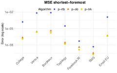
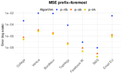
Figure 1: Mean Squared Error for a subset of the experiments ($\varepsilon=0.05,c=4$) for the progressive algorithms.

Experiment 2: Correlation to the exact betweenness rankings.

In this experiment, we measure how well our progressive algorithms can approximate the exact node rankings. In Figure 2 we show: the weighted Kendall’s tau, and the intersection between the Top-$50$ nodes of the rankings. We observe that all the algorithms perform very close on almost all the networks. p-ob, and p-trk provide less accurate rankings than p-rtb on Facebook and SMS. However, for these two networks p-rtb has the biggest sample size and the highest running time (see Table 2). This result suggests that these networks have a particular topology, where a lot of couples $(s,z)\in V\times V$ are not temporally connected, (see the additional materials for the temporal-connectivity analysis of these networks).

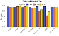
(a)

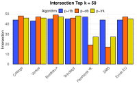
(b)

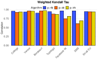
(c)

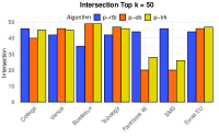
(d)

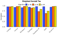
(c)

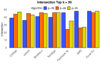
(d)

Figure 2: Weighted Kedall’s Tau and Intersection between the Top $50$ nodes in the exact ranking and the approximated ones (with parameters $\varepsilon=0.05,c=4$) for the: (1) shortest-temporal betweenness (a-b); prefix-foremost-temporal betweenness; (2) shortest-foremost-temporal betweenness (c-d); and, (3) prefix-foremost temporal betweenness (e-f).

Shortest-temporal betweenness Ratio runtime apx/exact Sample size Absolute Supremum Deviation $(\times 10^{-3})$ Mean Squared Error $(\times 10^{-6})$ Graph $\varepsilon$ $c$ p-rtb p-ob p-trk p-rtb p-ob p-trk p-rtb p-ob p-trk p-rtb p-ob p-trk Venice 0.1 2 0.025 0.17 0.11 20 1045 768 363.981 17.488 11.91 4195.3355 6.5405 3.4367 0.07 3 0.031 0.29 0.2 27 1881 1408 424.234 9.435 11.144 4263.5364 3.144 2.5459 0.05 4 0.047 0.52 0.38 33 3353 2560 399.63 8.643 8.966 3701.6107 1.9098 1.7596 Bord. 0.1 2 0.003 0.048 0.028 9 1045 816 740.489 18.214 8.695 8027.8714 10.8163 5.4813 0.07 3 0.004 0.094 0.05 16 1881 1594 907.617 14.953 15.632 7691.8831 6.2479 3.1767 0.05 4 0.008 0.163 0.09 27 3353 2746 646.911 14.51 10.924 6178.9318 3.5331 1.7887 Topol. 0.1 2 0.008 0.026 0.031 25 870 869 352.151 6.972 4.156 29.5556 0.0822 0.0459 0.07 3 0.014 0.041 0.054 50 1567 1514 233.788 12.136 8.589 21.1338 0.0555 0.0245 0.05 4 0.019 0.068 0.092 59 2794 2645 229.267 4.598 4.785 20.7994 0.0246 0.012 SMS 0.1 2 0.053 0.007 0.01 2042 504 741 3.991 1.993 0.704 0.0039 0.0009 0.0006 0.07 3 0.103 0.015 0.017 3362 907 1237 3.551 2.163 1.111 0.0033 0.0025 0.0003 0.05 4 0.118 0.018 0.027 4029 1617 2026 3.989 1.183 0.695 0.0038 0.0005 0.0002 Fb. W. 0.1 2 0.072 0.016 0.029 903 604 736 8.847 4.205 0.719 0.0418 0.0162 0.0042 0.07 3 0.105 0.029 0.05 1251 1088 1232 9.72 2.338 1.865 0.0453 0.0068 0.0029 0.05 4 0.162 0.047 0.082 1647 1940 2021 9.874 1.549 1.53 0.0418 0.0044 0.0014 Em. EU 0.1 2 0.042 0.118 0.047 30 870 714 322.816 8.579 7.837 353.8641 1.1537 0.6054 0.07 3 0.070 0.199 0.080 41 1306 1280 339.077 5.601 4.727 348.4084 0.622 0.3519 0.05 4 0.096 0.484 0.130 61 2794 2106 268.828 5.164 5.275 303.6608 0.3631 0.2337 Col. m. 0.1 2 0.094 0.194 0.154 59 870 672 116.026 11.32 5.885 89.6544 0.6974 0.3147 0.07 3 0.165 0.238 0.277 83 1306 1189 131.563 8.225 5.955 99.297 0.396 0.1931 0.05 4 0.233 0.415 0.460 118 2328 1989 109.146 4.813 3.673 84.167 0.2057 0.1084

Table 2: Runtime, sample size, absolute error and mean squared error for the shortest-temporal betweenness.

6 Concluding Remarks

We presented a suite of random sampling-based algorithms for computing high quality approximations of several notions of temporal betweenness centrality of all nodes in temporal graphs. We showed that, results on the sample size for the static betweenness can be extended to the shortest-temporal betweenness by considering the static-expansion of the temporal graph. Furthermore, we proposed two new approaches (rtb, trk) and refined the state-of-the-art technique (ob) by giving a sample complexity analysis and by defining their respective progressive-sampling versions. Our experiments show the effectiveness of these approaches for both approximating the temporal betweenness values and the rankings. An interesting future direction is to define a balanced bidirectional temporal bfs approach as for the static case to speedup the computation of the trk as in [13] and ob as in [18]. Other theoretical research directions include finding sharper bounds on the sample size for every optimality criteria and checking whether sample variance techniques [17, 18] can be extended to the temporal setting. Finally, extending our work to the temporal-walk based betweenness [10] appears to be a natural step to be taken to approximate all the meaningful variants of temporal betweenness centrality.

Additional Materials

Appendix A Implementation details.

We implemented all the algorithms in Julia exploiting multi-threading. We chose to re-implement the exact algorithms and Onbra because the available implementations of the exact algorithms have issues with the number of paths in the tested networks, causing overflow errors (indicated by negative centralities). Since Onbra is based on the shortest temporal betweenness code, it results in the same errors. Our implementation uses a sparse matrix representation of of the $|V|\times|T|$ table used in [9, 11], making the implemented algorithms space-efficient and allowing to compute the exact temporal shortest betweenness on big temporal graphs (for which the original version of the code gives out of memory errors). Furthermore, we noticed another error in the exact algorithms, related to time relabeling causing an underestimation of centralities.

Appendix B Useful mathematical tools

Here we list the mathematical tools used in this paper.

B.0.1 Concentration inequalities.

Theorem 11 (Hoeffding’s inequality)

Let $X_{1},\dots,X_{n}$ be independent bounded random variables with $a_{i}\leq X_{i}\leq b_{i}$, where $-\infty<a_{i}\leq b_{i}<\infty$ for all $i$ and $\mu=\textbf{E}\left[\sum_{i=1}^{n}\frac{x_{i}}{n}\right]$. Then

$${\textbf{Pr}}\left(\left|\frac{1}{n}\sum_{i=1}^{n}{\left(X_{i}-\textbf{E}\left[X_{i}\right]\right)}\right|\geq\xi\right)\leq 2\exp{\left(-\frac{2n^{2}\xi^{2}}{\sum_{i=1}^{n}{\left(b_{i}-a_{i}\right)^{2}}}\right)}$$ (3)

for all $\xi\geq 0$.

Theorem 12 (Chebyshev’s inequality)

For any $a>0$,

$${\textbf{Pr}}\left(\left|X-\textbf{E}\left[X\right]\right|\geq a\right)\leq\frac{{\textbf{Var}}\left[X\right]}{a^{2}}$$ (4)

B.0.2 Range Sets and Vapnik-Chervonenkis dimension.

A range space is a pair $\mathcal{R}=(X,\mathcal{I})$, where $X$ is a domain (finite or infinite) and $\mathcal{I}$ is a collection of subsets of $X$, called ranges. For a given $S\subseteq X$, the projection of $I$ on $S$ is the set $\mathcal{I}_{S}=\{S\cap I:I\in\mathcal{I}\}$. If $|\mathcal{I}_{S}|=2^{|S|}$ then we say $S$ is shattered by $\mathcal{I}$. The Vapnik-Chervonenkis dimension (VC-Dimension) of a range space is the size o the largest subset $S$ that can be shattered by $\mathcal{I}$.

Definition 7 (VC-dimension)

The VC-dimension of a range space $\mathcal{R}=(X,\mathcal{I})$, denoted by $\texttt{VC}(\mathcal{R})$ is

$$\texttt{VC}(\mathcal{R})=\max\{d:\exists S\subseteq X\land|S|=d\land|\mathcal{I}_{S}|=2^{d}\}$$

B.0.3 Pseudo-dimension.

Let $\mathcal{F}$ be a family of functions from some domain $\mathcal{D}$ to the range $[0,1]$. Consider $H=\mathcal{D}\times[0,1]$ . For each $f\in\mathcal{F}$, there is a subset $R_{f}\subseteq H$ defined as $R_{f}=\{(x,\alpha):x\in\mathcal{D}\land\alpha\leq f(x)\}$.

Definition 8

Let $\mathcal{R}=(\mathcal{D},\mathcal{F})$ and $\mathcal{R}^{\prime}=(H,\mathcal{F}^{+})$ be range spaces, where $\mathcal{F}^{+}={R_{f}:f\in\mathcal{F}}$. The pseudo-dimension of $\mathcal{R}$ denoted by $PD(\mathcal{R})$, corresponds to the VC-dimension of $\mathcal{R}^{\prime}$, i.e., $PD(\mathcal{R})=VC(\mathcal{R}^{\prime})$

The following theorem states that having an upper bound to the Pseudo-dimension of a range spaces allows to build an $(\varepsilon,\delta)$-approximation set.

Theorem 13

Let $\mathcal{R}^{\prime}=(H,\mathcal{F}^{+})$ be a range space (where $H=\mathcal{D}\times[0,1]$) with $\texttt{VC}(\mathcal{R}^{\prime})\leq d$ and a probability distribution $\pi$ on $\mathcal{D}$. Given $\varepsilon,\delta\in(0,1)$, and an universal constant $c$, let $S\subseteq H$ be a collection of elements sampled w.r.t. $\pi$. If we take $S$ such that $|S|=\frac{c}{\varepsilon^{2}}[d+\ln(\frac{1}{\delta})]$, then $S$ produces an $(\varepsilon,\delta)$-approximation set.

Appendix C Omitted proofs

Here we provide the proofs for lemmas and theorems that have not been included in the paper.

C.1 Bound on the sample size

A standard approach is to use the Hoeffeding’s inequality and union bound as follows. Given a temporal graph $\mathcal{G}=(V,\mathcal{E})$ with a straightforward application of the Hoeffding’s inequality [22], it is possible to show that,

$${\textbf{Pr}}\left(|\texttt{tb}^{(\star)}(v)-\widetilde{\texttt{tb}}^{(\star)}_{A}(v)|\geq\varepsilon\right)\leq 2e^{-2r\varepsilon^{2}}$$

If we fix $\delta=2e^{-2r\varepsilon^{2}}$, the error is $\varepsilon=\sqrt{\frac{\log(2/\delta)}{2r}}$, and the minimum $r$ needed to obtain an error $\varepsilon$ on the temporal betweenness of a single node is $\frac{1}{2\varepsilon^{2}}\log(2/\delta)$. The union-bound on all the nodes $v\in V$ gives

$${\textbf{Pr}}\left(\bigcup_{u\in V}\left[|\texttt{tb}^{(\star)}(v)-\widetilde{\texttt{tb}}^{(\star)}_{A}(v)|\geq\varepsilon\right]\right)\leq 2ne^{-2r\varepsilon^{2}}$$

Such inequality tells us that our procedure can safely sample $r=\frac{1}{2\varepsilon^{2}}\log\left(\frac{2n}{\delta}\right)$ nodes and produce an estimate of the $(\star)$-temporal betweenness of every node that is correct up to an additive error $\varepsilon$ with probability $1-\delta$. Next, we extend the result in [12] to the shortest-temporal betweenness centrality. Given a temporal graph $\mathcal{G}=(V,\mathcal{E})$ let $\mathcal{D}=\mathbb{TP}^{(sh)}_{\mathcal{G}}$, for each vertex appearance $(v,t)\in V\times T$, let $\uptau_{(v,t)}=\{tp\in\mathcal{D}:(v,t)\in\texttt{Int}(tp)\}$. For a pair $(s,z)\in V\times V$ and a temporal path $tp_{sz}\in\mathcal{D}$ let $f((v,t)|s,z)=f_{(v,t)}:\mathcal{D}\rightarrow[0,1]$ be the function $f_{(v,t)}(tp_{sz})=\mathds{1}{[(v,t)\in\textbf{{Int}}(tp_{sz})]}$ next, define $\mathcal{F}=\{f_{(v,t)}:(v,t)\in V\times T\}$, and $H=\mathcal{D}\times[0,1]$. For each $f_{(v,t)}\in\mathcal{F}$ there is a range $R_{(v,t)}=R_{f_{(v,t)}}=\{(tp_{sz},\alpha):tp_{sz}\in\mathcal{D}\land\alpha\leq f_{(v,t)}(tp_{sz})\}$. Define $\mathcal{F}^{+}=\{R_{(v,t):f_{(v,t)}\in\mathcal{F}}\}$ and let $R^{\prime}=(H,\mathcal{F}^{+})$

Theorem 14

Let $\mathcal{R}=(\mathcal{D},\mathcal{F})$ and $\mathcal{R}^{\prime}=(H,\mathcal{F}^{+})$ be the re corresponding range spaces for the domain and range set defined in before, and let $\text{VD}^{(sh)}(\mathcal{G})$ be the Vertex Diameter of $\mathcal{G}=(V,\mathcal{E})$ considering shortest-temporal as a temporal path optimality criterion. We have

$$PD(\mathcal{R})=VC(\mathcal{R}^{{}^{\prime}})\leq\lfloor\log\text{VD}^{(sh)}(\mathcal{G})-2\rfloor+1$$

Proof:

Let $VC(\mathcal{R}^{{}^{\prime}})=d$, where $d\in\mathbb{N}$. Then, there is $S\subset H$ such that $|S|=d$ and $S$ is shattered by $\mathcal{F}^{+}$. For each temporal path $tp_{sz}\in\mathcal{D}$, there is at most one pair $(tp_{sz},\alpha)$ in $S$ for some $\alpha\in(0,1]$ and there is no pair of the form $(tp_{sz},0)$. By definition of shattering, each $(tp_{sz},\alpha)\in S$ appears in $2^{d-1}$ different ranges in $\mathcal{F}^{+}$. Moreover, each pair $(tp_{sz},\alpha)$ is in at most $|tp_{sz}|-2$ ranges in $\mathcal{F}^{+}$, that is because $(tp_{sz},\alpha)\notin R_{v,t}$ either when $\alpha>f_{(v,t)}(tp_{sz})$ or $(v,t)\notin tp_{sz}$. Observe that $|tp_{sz}|-2\leq\text{VD}^{(sh)}(\mathcal{G})-2$, gives

$$2^{d}\leq|tp_{sz}|-2\leq\text{VD}^{(sh)}(\mathcal{G})-2$$

thus,

$$d-1\leq\log(\text{VD}^{(sh)}(\mathcal{G})-2)$$

since $d\in\mathbb{N}$, we have

$$d\leq\lfloor\log\text{VD}^{(sh)}(\mathcal{G})-2\rfloor+1\leq\log(\text{VD}^{(sh)}(\mathcal{G})-2)+1$$

Finally,

$$PD(\mathcal{F})=VC(\mathcal{F}^{+})=d\leq\lfloor\log\text{VD}^{(sh)}(\mathcal{G})-2\rfloor+1$$

$\square$

C.2 Random Temporal Betweenness estimator

Lemma 3

The rtb is an unbiased estimator of the $(\star)$-temporal betweenness centrality.

Proof:

$$\textbf{E}\left[f^{(\star)}_{\texttt{{rtb}}}(v|s)\right]=\sum_{s\in V}{\textbf{Pr}}\left(s\right)\cdot f^{(\star)}_{\texttt{{rtb}}}(v|s)=\sum_{s\in V}\frac{1}{n}\left(\frac{1}{n-1}\sum_{z\neq s\neq v}{\frac{\sigma^{(\star)}_{sz}(v)}{\sigma^{(\star)}_{sz}}}\right)$$

$\square$
To analyze the adaptive approach, we use the following lemmas.

Lemma 4

$\textbf{E}\left[f^{(\star)}_{\texttt{{p-rtb}}}(v|v_{i})\right]=\frac{1}{n}\sum_{i\in[n]}f^{(\star)}_{\texttt{{p-rtb}}}(v|v_{i})$, and ${\textbf{Var}}\left[f^{(\star)}_{\texttt{{p-rtb}}}(v|v_{i})\right]\leq\sum_{i\in[n]}f^{(\star)}_{\texttt{{p-rtb}}}(v|v_{i})$.

Proof:

Let us start with computing the expected value of the random variable $f^{(\star)}_{\texttt{{p-rtb}}}(v|v_{i})$:

$$\textbf{E}\left[f^{(\star)}_{\texttt{{p-rtb}}}(v|v_{i})\right]=\sum_{i\in[n]}{\textbf{Pr}}\left(v_{i}\right)f^{(\star)}_{\texttt{{p-rtb}}}(v|v_{i})=\frac{1}{n}\sum_{i\in[n]}f^{(\star)}_{\texttt{{p-rtb}}}(v|v_{i})$$

Finally,

$${\textbf{Var}}\left[f^{(\star)}_{\texttt{{p-rtb}}}(v|v_{i})\right]=\textbf{E}\left[f^{(\star)}_{\texttt{{p-rtb}}}(v|v_{i})^{2}\right]-\textbf{E}\left[f^{(\star)}_{\texttt{{p-rtb}}}(v|v_{i})\right]^{2}\leq F$$

$\square$
Subsequently, we provide a lemma to compute the lower bound on the expected number of samples needed to satisfy the stopping condition.

Lemma 5

Assume $k=\varepsilon n^{2}/F$ then,

$${\textbf{Pr}}\left(\sum_{i\in[k]}f^{(\star)}_{\texttt{{p-rtb}}}(v|v_{i})\geq c\cdot n\right)\leq\frac{\varepsilon}{(c-\varepsilon)^{2}}$$ (5)

Proof:

$${\textbf{Pr}}\left(\sum_{i\in[k]}f^{(\star)}_{\texttt{{p-rtb}}}(v|v_{i})\geq cn\right)={\textbf{Pr}}\left(\sum_{i\in[k]}\left(f^{(\star)}_{\texttt{{p-rtb}}}(v|v_{i})-\frac{F}{n}\right)\geq cn-\frac{kF}{n}\right)$$

$$={\textbf{Pr}}\left(\sum_{i\in[k]}\left(f^{(\star)}_{\texttt{{p-rtb}}}(v|v_{i})-\frac{F}{n}\right)\geq cn-\varepsilon n\right)\leq$$

$$\sum_{i\in[k]}{\textbf{Pr}}\left(f^{(\star)}_{\texttt{{p-rtb}}}(v|v_{i})-\frac{F}{n}\geq n(c-\varepsilon)\right)\leq\text{ (Chebychev's ineq.)}$$

$$\frac{1}{n^{2}(c-\varepsilon)^{2}}\sum_{i\in[k]}{\textbf{Var}}\left[f^{(\star)}_{\texttt{{p-rtb}}}(v|v_{i})\right]\leq\frac{kF}{n^{2}(c-\varepsilon)^{2}}=\frac{\varepsilon}{(c-\varepsilon)^{2}}$$

$\square$

Lemma 6

Let $k\geq\varepsilon n^{2}/F$ ad $\alpha>0$. Then

$${\textbf{Pr}}\left(\left|\frac{n}{k}\cdot\left(\sum_{i\in[k]}f^{(\star)}_{\texttt{{p-rtb}}}(v|v_{i})\right)-F\right|\geq\alpha\cdot F\right)\leq\frac{1}{\varepsilon\cdot\alpha^{2}}$$ (6)

Proof:

$${\textbf{Pr}}\left(\left|\frac{n}{k}\left(\sum_{i\in[k]}f^{(\star)}_{\texttt{{p-rtb}}}(v|v_{i})\right)-F\right|\geq\xi F\right)={\textbf{Pr}}\left(\left|\left(\sum_{i\in[k]}f^{(\star)}_{\texttt{{p-rtb}}}(v|v_{i})\right)-\frac{k}{n}F\right|\geq\frac{k}{n}\xi F\right)=$$

$${\textbf{Pr}}\left(\left|\left(\sum_{i\in[k]}f^{(\star)}_{\texttt{{p-rtb}}}(v|v_{i})-\frac{1}{n}F\right)\right|\geq\frac{k}{n}\xi F\right)\leq\frac{n^{2}}{k^{2}\xi^{2}}k{\textbf{Var}}\left[f^{(\star)}_{\texttt{{p-rtb}}}(v|v_{i})\right]$$

Let $k=\beta n^{2}/F$, with $\beta\geq\varepsilon$. Then we have that the above probability is less or equal to

$$\frac{n^{2}}{k^{2}\xi^{2}}k{\textbf{Var}}\left[f^{(\star)}_{\texttt{{p-rtb}}}(v|v_{i})\right]\leq\frac{n^{2}}{\beta\frac{n^{2}}{F}\xi^{2}}F=\frac{F^{2}}{\beta\xi^{2}}$$

Setting $F\xi=\alpha$ gives $\frac{1}{\beta\alpha^{2}}\leq\frac{1}{\varepsilon\alpha^{2}}$. $\square$
Given these three lemmas we can prove Theorems 15, and 16.

Theorem 15

Let $\hat{F}$ be the estimate of $F$, and let $F>0$. Then Heuristic $1$ estimates $F$ to within a factor of $1/\varepsilon$ for $0<\varepsilon<\frac{1}{2}$ with probability at least $1-2\varepsilon$.

Proof:

First, we show that it is unlikely that the algorithm stops too early to guarantee a good error bound.

$${\textbf{Pr}}\left(\exists j:j\leq k\land\sum_{i\in[j]}f^{(\star)}_{\texttt{{p-rtb}}}(v|v_{i})\geq cn\right)\leq{\textbf{Pr}}\left(\sum_{i\in[k]}f^{(\star)}_{\texttt{{p-rtb}}}(v|v_{i})\geq cn\right)$$

Where $k=\frac{\varepsilon n^{2}}{F}$. By Lemma 5, the right side of the inequality is at most $\frac{\varepsilon}{(c-\varepsilon)^{2}}$, taking $c=2$ and noticing that $0<\varepsilon<\frac{1}{2}$ we get that this probability is less than $\varepsilon$. Subsequently, we show that it is unlikely that the algorithm stops after enough samples but with bad estimate. If $k=\frac{\varepsilon n^{2}}{F}$, then by Lemma 6 $\hat{F}=\frac{n}{k}\sum_{i\in[k]}f^{(\star)}_{\texttt{{p-rtb}}}(v|v_{i})$ is within $\alpha F$ of $F$ with probability greater or equal to $1/(\varepsilon\alpha^{2})$, Letting $\alpha=1/\varepsilon$, this is just $\varepsilon$. Now, we can bound the probability that the algorithm “fails” as

$${\textbf{Pr}}\left(\text{``The Algorithm fails''}\right)\leq\varepsilon+(1-\varepsilon)\varepsilon<2\varepsilon$$

$\square$

Theorem 16

For $0<\varepsilon<\frac{1}{2}$, if the centrality of a vertex $v$ is $\frac{n^{2}}{t}$ for some constant $t\geq 1$, then Heuristic $1$ with probability at least $1-2\varepsilon$ estimates its betweenness centrality within a factor $\frac{1}{\varepsilon}$ using $\varepsilon\cdot t$ sample nodes.

Proof:

In order to prove this theorem, let $F=\frac{n^{2}}{t}$ and repeat the same analysis of Theorem 15. $\square$

C.3 ONBRA estimator

Lemma 7

The function computed by ob is an unbiased estimator of the $(\star)$-temporal betweenness centrality.

Proof:

$$\textbf{E}\left[f^{(\star)}_{\texttt{{ob}}}(v|s,z)\right]=\sum_{\begin{subarray}{c}s,z\in V\\ s\neq z\end{subarray}}{\textbf{Pr}}\left((s,z)\right)f^{(\star)}_{\texttt{{ob}}}(v|s,z)=\sum_{\begin{subarray}{c}s,z\in V\\ s\neq z\end{subarray}}\frac{1}{n(n-1)}\frac{\sigma_{sz}^{(\star)}(v)}{\sigma_{sz}^{(\star)}}$$

$\square$

Theorem 17

The progressive algorithm is an $(\varepsilon,\delta)$-approximation algorithm for the $(\star)$-temporal Betweenness Centrality.

Proof:

Let $j$ be the number of iterations of the while loop (lines 6-18) of Algorithm $1$ in Section $4$. Take the sample $S_{j}=\{(s_{1},z_{1}),\dots,(s_{r},z_{r})\}$ of size $r$ obtained after the last iteration of the loop where the stopping condition is satisfied. Let $\xi_{j}$ be the value obtained at line 16 on the $i^{th}$ iteration and let $\omega(s)$ be the upper bound to the empirical Rademacher average of the sample $S_{i}$ computed by minimizing the function defined in Theorem $2$ (see Section 3). Then $\xi_{j}$ is such that $\xi_{j}\leq\varepsilon$ for the temporal graph in input and for the fixed constants $\varepsilon,\delta\in(0,1)$. Define $X_{i}\in\{0,1\}$ as the random variable that assumes value $1$ if $\sup_{v\in V}|\texttt{tb}^{(\star)}(v)-\widetilde{\texttt{tb}}^{(\star)}(v)|>\xi_{i}$ at iteration $i$. We need that $X_{i}$ assumes value $1$ with probability $\delta$. Thus, we need

$${\textbf{Pr}}\left(\exists i\geq 1,\;X_{i}=1\right)={\textbf{Pr}}\left(\bigcup_{i\geq 1}{\textbf{Pr}}\left(X_{i}=1\right)\right)\leq\sum_{i\geq 1}{\textbf{Pr}}\left(X_{i}=1\right)\leq\delta$$

Setting ${\textbf{Pr}}\left(X_{i}=1\right)=\delta/2^{i}$, we have

$$\sum_{i\geq 1}{\textbf{Pr}}\left(X_{i}=1\right)=\delta\sum_{i\geq 1}\frac{1}{2^{i}}=\delta$$

At each iteration $i$, the pair $(s_{l},z_{l})$ is sampled with uniform probability over $\mathcal{D}_{\texttt{{ob}}}$, for $l\in[r]$ and the set $\Gamma_{s_{l},z_{l}}^{(\star)}$ is computed by the $(\star)$-temporal bfs (line 11). The value ${\sigma_{s_{l}z_{l}}^{(\star)}(v)}/{\sigma_{s_{l}z_{l}}^{(\star)}}$ is computed by the backtracking procedure [11]. The computed value is an unbiased estimator of the $(\star)$-temporal betweenness centrality (Lemma 7). Since $\xi_{j}\leq\varepsilon$, then $L_{\mathcal{S}_{j}}(f^{(\star)}_{\texttt{{ob}}}(v))=\widetilde{\texttt{tb}}^{(\star)}(v)$ and $L_{\mathcal{D}_{\texttt{{ob}}}}(f^{(\star)}_{\texttt{{ob}}}(v))=\texttt{tb}^{(\star)}(v)$, then by Theorem 2 in Section $2$, we have ${\textbf{Pr}}\left(|\texttt{tb}^{(\star)}(v)-\widetilde{\texttt{tb}}^{(\star)}(v)|\leq\varepsilon\right)\geq 1-\delta$. $\square$

C.4 Temporal Riondato and Kornaropoulos estimator

Theorem 18

Let $tp^{*}_{sz}\in\Gamma_{sz}^{(\star)}$ be the $(\star)$-temporal path sampled using the above procedure. Then, the probability of sampling $tp^{*}_{sz}$ is ${\textbf{Pr}}\left(tp^{*}\right)=\frac{1}{\sigma^{(\star)}_{sz}}$

Proof:

Let $\sigma_{sz}=\sigma_{sz}^{(\star)}$. The probability of getting such $tp^{*}$ using the aforementioned temporal path sampling technique is:

$${\textbf{Pr}}\left(tp^{*}\right)=\frac{\sigma_{sz}^{t_{z}}}{\sum_{t}\sigma_{sz}^{t}}\cdot\frac{\sigma_{sw_{k-1}}^{t_{w_{k-1}}}}{\sum_{(x,t)\in P(z,t_{z})}\sigma_{sx}^{t}}\cdot\frac{\sigma_{sw_{k-2}}^{t_{w_{k-2}}}}{\sum_{(x,t)\in P(w_{k-1},t_{k-1})}\sigma_{sx}^{t}}\cdots\frac{\sigma_{sw_{1}}^{t_{w_{1}}}}{\sum_{(x,t)\in P(w_{2},t_{2})}\sigma_{sx}^{t}}\cdot\frac{1}{\sum_{(x,t)\in P(w_{1},t_{1})}\sigma_{sx}^{t}}$$

Observe that $\sigma_{sw}^{t_{w}}=\sum_{(x,t)\in P(w,t_{w})}\sigma_{sx}^{t}$ and that $\sum_{t}\sigma_{sz}^{t}=\sigma_{sz}$. Thus, the formula can be rewritten as follows:

$${\textbf{Pr}}\left(tp^{*}\right)=\frac{\sigma_{sz}^{t_{z}}}{\sigma_{sz}}\cdot\frac{\sigma_{sw_{k-1}}^{t_{w_{k-1}}}}{\sigma_{sz}^{t_{z}}}\cdots\frac{1}{\sigma_{sw_{1}}^{t_{w_{1}}}}=\frac{1}{\sigma_{sz}}$$

and the fact that (if the temporal graph has no self loop) for $(w_{1},t_{w_{1}})$, which is a temporal neighbor of $(s,0)$, $\sigma_{sw_{1}}=1$. $\square$

Theorem 19

The function $\pi_{\texttt{{trk}}}(tp_{sz})$, for each $tp_{sz}\in\mathcal{D}_{\texttt{{trk}}}$, is a valid probability distribution.

Proof:

Let $\Gamma_{sz}^{(\star)}$ be the set of $(\star)$-optimal temporal paths from $s$ to $z$ where $s\neq z$. Then,

$$\sum_{tp_{sz}\in\mathcal{D}_{\texttt{{trk}}}}\pi(tp_{sz})=\sum_{tp_{sz}\in\mathcal{D}_{\texttt{{trk}}}}\frac{1}{n(n-1)}\frac{1}{\sigma_{sz}^{(\star)}}= \sum_{s\in V}\sum_{\begin{subarray}{c}z\in V\\ s\neq z\end{subarray}}\sum_{tp_{sz}\in\Gamma_{sz}^{(\star)}}\frac{1}{n(n-1)}\frac{1}{\sigma_{sz}^{(\star)}}=\sum_{s\in V}\sum_{\begin{subarray}{c}z\in V\\ s\neq z\end{subarray}}\frac{1}{n(n-1)}\frac{\sigma_{sz}^{(\star)}}{\sigma_{sz}^{(\star)}}$$

$$=\frac{1}{n(n-1)}\sum_{s\in V}\sum_{\begin{subarray}{c}z\in V\\ s\neq z\end{subarray}}1=\frac{1}{n(n-1)}\sum_{s\in V}(n-1)=1$$

$\square$

Theorem 20

For $f^{(\star)}_{\texttt{{trk}}}(v)\in\mathcal{F}$ and for all $tp_{sz}\in\mathcal{D}_{\texttt{{trk}}}$, such that each $tp_{sz}$ is sampled according to the probability function $\pi(tp_{sz})$, then $\textbf{E}\left[f^{(\star)}_{\texttt{{trk}}}(v|tp_{sz})\right]=\texttt{tb}^{(\star)}(v)$.

Proof:

$$\textbf{E}_{tp_{sz}\in\mathcal{D}_{\texttt{{trk}}}}\left[f^{(\star)}_{\texttt{{trk}}}(v|tp_{sz})\right]=\sum_{tp_{sz}\in\mathcal{D}_{\texttt{{trk}}}}\pi(tp_{sz})f^{(\star)}_{\texttt{{trk}}}(v|tp_{sz})=\sum_{tp_{sz}\in\mathcal{D}_{\texttt{{trk}}}}\frac{1}{n(n-1)\sigma_{sz}^{(\star)}}f^{(\star)}_{\texttt{{trk}}}(v|tp_{sz})$$

$$=\frac{1}{n(n-1)}\sum_{\begin{subarray}{c}s\in V\\ s\neq v\end{subarray}}\sum_{\begin{subarray}{c}z\in V\\ z\neq s\neq v\end{subarray}}\sum_{tp\in\Gamma_{sz}^{(\star)}}\frac{\mathds{1}\left[v\in\textbf{ Int}(tp)\right]}{\sigma^{(\star)}_{sz}}=\frac{1}{n(n-1)}\sum_{\begin{subarray}{c}s\in V\\ s\neq v\end{subarray}}\sum_{\begin{subarray}{c}z\in V\\ z\neq s\neq v\end{subarray}}\frac{\sigma^{(\star)}_{sz}(v)}{\sigma^{(\star)}_{sz}}$$

$\square$

Appendix D Estimating the shortest temporal diameter

Given a temporal graph $\mathcal{G}=(V,\mathcal{E})$, let $N(u,h)=\{v\in V:d(u,v)\leq h\}$ be the temporal ball centered in $u$ at time $0$ of radius $h$. $N(u,h)$ is the set of all the nodes $v$ that can be reached by node $u$ starting at time $0$ and that requires the smallest number of time respecting hops. Now define $|N(h)|=|\{(u,v)\in V\times V:d(u,v)\leq h\}|$ as the set of pairs of nodes within shortest temporal distance $h$. The shortest-temporal diameter $D$ of a graph is the longest shortest temporal path in the temporal graph. In terms of $N(h)$ we have:

$$D=\min_{h}\left(h:\sum_{u}|N(u,h)|=\sum_{u}|N(u,h+1)|\right)$$

Alternatively, as for the static case, we can define the effective shortest temporal diameter as the $\tau^{(th)}$ percentile shortest temporal distance between the nodes. Let $\tau\in[0,1]$, then

$$D_{\tau}=\min_{h}\left(h:\frac{\sum_{u}|N(u,h)|}{\sum_{u}|N(u,D)|}\geq\tau\right)$$

Next, we define the overall temporal connectivity rate of a temporal graph $\mathcal{G}=(V,\mathcal{E})$ as

$$\zeta(\mathcal{G})=\frac{\sum_{\begin{subarray}{c}u,v\in V\\ u\neq v\end{subarray}}\mathds{1}[u\rightsquigarrow v]}{n(n-1)}\in[0,1]$$

where $u\rightsquigarrow v$ stands for “there is at least one shortest temporal path between $u$ and $v$”. Notice that this is a measure that gives insight about “how temporally connected $\mathcal{G}$ is”. Finally, observe that given $N(u,h)$ for each $u\in V$ and $h\in\{0,\dots,D\}$ we can define the average shortest-temporal distance

$$\texttt{AvgDist}=\frac{\sum_{\begin{subarray}{c}u,v\in V\\ u\neq v\end{subarray}}\mathds{1}[u\rightsquigarrow v]\cdot d(u,v)}{\sum_{\begin{subarray}{c}u,v\in V\\ u\neq v\end{subarray}}\mathds{1}[u\rightsquigarrow v]}=\frac{\sum_{u\in V}\sum_{h\in[D]}(|N(u,h)-|N(u,h-1))\cdot h}{|N(D)|}$$

Algorithm 3, computes the shortest temporal distance-based metrics described above. Moreover, we can give a bound on the quality of the approximation produced by this approach.

Theorem 21

Given a temporal graph $\mathcal{G}=(V,\mathcal{E})$ and a sample of size $s=\Theta\left(\frac{\ln n}{\varepsilon^{2}}\right)$. Algorithm 3 computes with probability $1-\frac{2}{n^{2}}$ the shortest (effective) temporal diameter with absolute error bounded by $\varepsilon\over\zeta(\mathcal{G})$, the temporal connectivity rate $\zeta(\mathcal{G})$ with absolute error bounded by $\varepsilon$, and the average shortest temporal distance with absolute error bounded by $\frac{\varepsilon\cdot D}{\zeta(\mathcal{G})}$.

Proof:

Let $h$ be the shortest temporal effective diameter threshold, and

$$X_{i}^{h}=\frac{n\cdot\sum_{\{u:d(v_{i},u)\leq h\}}\mathds{1}[v_{i}\rightsquigarrow u]}{\sum_{\begin{subarray}{c}u,v\in V\\ u\neq v\end{subarray}}\mathds{1}[u\rightsquigarrow v]}=\frac{n\cdot|N(v_{i},h)|}{|N(D)|}$$

observe that $X_{i}^{h}\in[0,\frac{1}{\zeta}]$, and that $X_{i}^{h}$’s expected value is

$$\textbf{E}\left[X_{i}^{h}\right]=\sum_{v_{i}\in V}X_{i}^{h}\cdot{\textbf{Pr}}\left(v_{i}\right)=\frac{\sum_{v_{i}\in V}|N(v_{i},h)|}{|N(D)|}=\frac{|N(h)|}{|N(D)|}$$

Applying Hoeffding’s inequality, with $\xi=\frac{\varepsilon}{\zeta}$, we can approximate $\frac{|N(h)|}{|N(D)|}$ by $\frac{\sum_{i\in[s]}X_{i}^{h}}{s}=\frac{n\cdot\sum_{i\in[s]}|N(u,v_{i})|}{s\cdot|N(D)|}$, and taking a sample of $s={\ln n\over\varepsilon^{2}}$ leads an error of $\varepsilon\over\zeta$ with probability of at least $1-\frac{2}{n^{2}}$. Now we observe that the shortest temporal diameter can be defined in terms of the effective one by choosing $\tau=1$, thus the bound holds also for the shortest temporal diameter. Next, define the random variable $X_{i}^{D}=\frac{|N(v_{i},D)|}{n-1}$, and observe that $X_{i}^{D}\in[0,1]$. Observe that its expected value is exactly $\zeta(\mathcal{G})$:

$$\textbf{E}\left[X_{i}^{D}\right]=\sum_{v_{i}\in V}\frac{1}{n}\frac{|N(v_{i},D)|}{n-1}=\frac{|N(D)|}{n(n-1)}=\zeta(\mathcal{G})$$

Again, applying Hoeffding’s inequality, with $\xi=\varepsilon$, and taking $s={\ln n\over\varepsilon^{2}}$ sample nodes, we have an error bound of $\varepsilon$ with high probability. Finally, define

$$X_{i}=\frac{n\cdot\sum_{u\in V}\mathds{1}[v_{i}\rightsquigarrow u]\cdot d(v_{i},u)}{\sum_{\begin{subarray}{c}u,v\in V\end{subarray}}\mathds{1}[u\rightsquigarrow v]}$$

Observe that $X_{i}\in[0,\frac{D}{\zeta(\mathcal{G})}]$, and that its expectation is the average shortest temporal distance

$$\textbf{E}\left[X_{i}\right]=\sum_{v_{i}\in V}X_{i}\cdot{\textbf{Pr}}\left(X_{i}\right)=\frac{\sum_{\begin{subarray}{c}v_{i},u\in V\end{subarray}}\mathds{1}[v_{i}\rightsquigarrow u]\cdot d(v_{i},u)}{\sum_{\begin{subarray}{c}u,v\in V\end{subarray}}\mathds{1}[u\rightsquigarrow v]}$$

Finally, by using Hoeffding’s inequality with $\xi=\frac{\varepsilon D}{\zeta(\mathcal{G})}$ and setting $s=\frac{\log n}{\varepsilon^{2}}$ we obtain that the error is of at most $\frac{\varepsilon D}{\zeta(\mathcal{G})}$ with probability $1-\frac{2}{n^{2}}$. $\square$

	Exact measures					Approximated measures
Graph	D	$\bm{D(\tau)}$	AvgDist	$\bm{\zeta}$		$\bm{\tilde{D}}$	$\bm{\tilde{D(\tau)}}$	$\widetilde{\texttt{AvgDist}}$	$\bm{\tilde{\zeta}}$
Venice	99	38.54	24.95	0.67		84	38.92	24.90	0.67
College msg	17	5.64	4.59	0.50		15	5.63	4.57	0.52
Email EU	13	4.50	3.80	0.79		13	4.55	3.90	0.79
Bordeaux	147	70.52	47.91	0.84		130	68.62	46.98	0.84
Topology	20	6.35	5.22	0.53		17	6.19	5.18	0.53
Facebook wall	34	14.77	10.38	0.04		27	14.82	10.42	0.04
SMS	32	13.15	9.25	0.001		22	13.06	9.25	0.001

Table 3: Exact and approximated values for the shortest temporal (effective) diameter, the temporal connectivity rate, and shortest temporal average distance.

Table 3 shows the exact and approximated shortest-temporal distance-based measures of the networks of interest. The sampling algorithm have been run $5$ times using $16$ threads and $64$ sample nodes. We observe that provides accurate estimations of the temporal-distance measures. In addition we notice that Facebook wall and SMS networks have very low temporal connectivity rate i.e., a lot of couples $(s,z)\in V\times V$ are not temporally connected. Thus justifying the poor performances of the sampling algorithms on these temporal graphs.

Appendix E Additional Experiments

In this section we show additional experiments for the progressive and for the fixed sample size algorithms.

E.1 Progressive algorithms: running time, estimation error, and rank correlation.

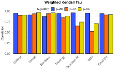
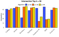
Figure 3: Weighted Kedall’s Tau and Intersection between the Top $50$ nodes in the exact ranking and the approximated ones (with parameters $\varepsilon=0.1,c=2$) for the shortest-foremost-temporal betweenness

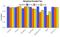
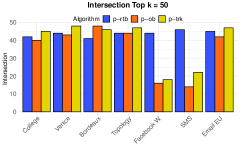
Figure 4: Weighted Kedall’s Tau and Intersection between the Top $50$ nodes in the exact ranking and the approximated ones (with parameters $\varepsilon=0.07,c=3$) for the shortest-foremost-temporal betweenness

Table 4 shows the running times in seconds of the progressive algorithms for all the considered temporal path optimality criteria. In Table 5 and 6 we show respectively the results of Experiment 1 for the shortest-foremost, and prefix-foremost temporal betwenness. We observe that as for the shortest-temporal betweenness (see Section $5$) the sample size of p-ob, and p-trkgrows as $\varepsilon^{-2}$, while p-rtb’s sample size seems to depend on how well temporally connected the network is. p-trk, turns to be method with the lowest absolute supremium deviation and mean squared error i.e., the best algorithm to approximate the temporal-betweenness values of the nodes. Figure 3, and Figure 4 show the weighted Kendall’s Tau correlation and Top-50 intersection between the exact shortest-foremost temporal betweenness rankings and the approximations computed using our methods. We observe that p-ob, and p-trk provide less accurate rankings than p-rtb on Facebook and SMS. However, for these two networks p-rtb has the biggest sample size and the highest running time. Moreover, rtb always provides good Top-50 approximations, while p-ob, and p-trk on some networks need a bigger sample size to find the Top-50 most influential nodes in the network.

		Execution time (seconds)
				Shortest					Shortest-foremost					Prefix-foremost
Graph	$\varepsilon$	$c$		Ex.	rtb	p-ob	p-trk		Ex.	rtb	p-ob	p-trk		Ex.	rtb	p-ob	p-trk
Venice	0.1	2		2499.1	62.1	427.1	289.3		2512.5	54.9	485.9	299.2		13.7	0.4	7.9	6.2
	0.07	3			78.4	719.3	523.1			59.9	789.5	584.3			0.7	12.9	11.4
	0.05	4			117.4	1303.3	962.5			124.1	1448.9	1050.9			1.0	22.7	20.6
Bord.	0.1	2		41540.5	105.3	1943.4	1165.4		41400.8	135.8	2851.2	1375.3		96.2	1.9	19.4	17.4
	0.07	3			159.4	3884.4	2184.5			159.9	5161.2	2502.2			3.6	37.2	34.0
	0.05	4			352.5	6766.9	3864.6			380.6	9806.6	4407.7			5.2	65.6	58.2
Topol.	0.1	2		5528.9	45.3	145.2	172.4		5586.5	64.2	144.0	213.6		209.5	1.2	12.8	13.8
	0.07	3			78.9	227.2	295.8			104.9	280.0	374.8			2.6	20.0	22.6
	0.05	4			106.7	374.6	511.3			147.2	480.9	630.6			4.1	35.6	40.6
SMS	0.1	2		17876.3	955.8	116.5	172.7		19263.0	838.7	119.0	184.7		253.6	14.0	3.2	4.7
	0.07	3			1849.0	262.7	305.2			1224.2	255.0	299.8			18.2	4.7	8.7
	0.05	4			2118.3	327.0	488.8			1570.7	441.6	502.3			28.7	8.9	13.9
FB.W.	0.1	2		1956.9	141.7	31.8	56.8		1958.1	98.3	33.2	59.4		165.9	7.1	0.9	4.3
	0.07	3			206.3	55.8	97.6			170.0	56.3	98.5			10.7	2.1	6.6
	0.05	4			316.1	92.4	160.5			222.9	100.7	160.7			25.1	5.2	12.0
Em.EU	0.1	2		20679.9	860.2	2430.7	967.2		20761.7	729.5	1513.9	952.7		36.8	2.2	29.9	24.4
	0.07	3			1437.7	4123.1	1653.9			1286.2	3852.9	1628.9			4.0	60.1	46.0
	0.05	4			1983.7	10003.1	2693.6			1577.5	7748.2	2595.1			6.7	106.1	82.9
Col. m.	0.1	2		223.1	21.1	43.3	34.4		222.3	23.6	43.8	39.6		3.9	0.3	10.1	1.7
	0.07	3			36.7	53.1	61.8			41.5	62.3	65.9			0.5	9.2	2.9
	0.05	4			52.1	92.7	102.5			59.1	94.6	110.8			0.7	11.2	4.6

Table 4: Running times in seconds of the exact (Ex.) and progressive algorithms for each data set and each temporal optimality criteria.

Shortest-foremost-temporal betweenness Ratio runtime apx/exact Sample size Absolute Supremum Deviation $(\times 10^{-3})$ Mean Squared Error $(\times 10^{-6})$ Graph $\varepsilon$ $c$ p-rtb p-ob p-trk p-rtb p-ob p-trk p-rtb p-ob p-trk p-rtb p-ob p-trk Venice 0.1 2 0.022 0.193 0.119 14 1045 768 517.6082 17.9608 13.0667 6597.2109 10.2849 5.6539 0.07 3 0.024 0.314 0.233 19 1881 1434 512.6649 11.6197 9.7198 5937.6089 4.3531 3.0261 0.05 4 0.049 0.577 0.418 30 3353 2576 533.7849 12.798 8.6949 6947.0973 2.6489 1.7432 Bord. 0.1 2 0.003 0.069 0.033 12 1254 816 634.5118 26.3619 10.5596 8075.0943 12.2513 3.7381 0.07 3 0.004 0.125 0.060 15 2257 1578 818.2244 14.1538 14.1788 10732.9756 5.5026 2.7754 0.05 4 0.009 0.237 0.106 29 4023 2752 503.9168 11.6003 9.7246 7888.0234 3.9171 2.2523 Topol. 0.1 2 0.011 0.026 0.038 31 870 821 256.3878 14.721 6.1906 20.6234 0.098 0.0399 0.07 3 0.019 0.050 0.067 44 1567 1509 278.5611 5.3999 4.9913 27.5715 0.0433 0.0246 0.05 4 0.026 0.086 0.113 55 2794 2565 319.4647 7.3454 4.1562 29.4967 0.0264 0.0154 SMS 0.1 2 0.044 0.006 0.010 1584 604 736 5.1949 4.1027 0.837 0.0045 0.0025 0.0005 0.07 3 0.064 0.013 0.016 2429 907 1237 5.0429 3.0319 0.6716 0.0045 0.0011 0.0002 0.05 4 0.082 0.023 0.026 3182 1617 2016 5.2207 0.9294 0.7042 0.0048 0.0003 0.0002 Fb. W. 0.1 2 0.050 0.017 0.030 722 604 736 11.4512 4.0136 1.9687 0.0583 0.0149 0.005 0.07 3 0.087 0.029 0.050 1132 1088 1232 10.6349 2.8733 0.9884 0.0532 0.0083 0.0021 0.05 4 0.114 0.051 0.082 1459 1088 2016 11.0998 1.943 0.7185 0.0506 0.004 0.0014 Em. EU 0.1 2 0.035 0.073 0.046 1170 870 693 374.4456 14.894 5.3508 1363.7046 1.638 0.7461 0.07 3 0.062 0.186 0.078 2708 1567 1184 384.1069 10.7663 9.0763 1504.3896 0.8493 0.624 0.05 4 0.076 0.373 0.125 4828 2794 1909 381.5071 11.3429 8.3383 1243.7985 0.5007 0.4429 Col. m. 0.1 2 0.106 0.197 0.178 43 870 677 161.13 8.7778 8.7017 170.8668 0.6939 0.3264 0.07 3 0.187 0.280 0.297 76 1567 1157 171.8233 11.3773 4.1759 158.2298 0.4616 0.2046 0.07 3 0.187 0.280 0.297 76 1567 1157 171.8233 11.3773 4.1759 158.2298 0.4616 0.2046 0.05 4 0.266 0.426 0.498 92 2328 1968 174.4413 4.241 5.738 162.1282 0.2261 0.1361

Table 5: Runtime, sample size, absolute error and mean squared error for the shortest-foremost-temporal betweenness.

Prefix-foremost-temporal betweenness Ratio runtime apx/exact Sample size Absolute Supremum Deviation $(\times 10^{-3})$ Mean Squared Error $(\times 10^{-6})$ Graph $\varepsilon$ $c$ p-rtb p-ob p-trk p-rtb p-ob p-trk p-rtb p-ob p-trk p-rtb p-ob p-trk Venice 0.1 2 0.03 0.58 0.45 9 1254 768 995.4701 25.2591 27.2997 13742.517 14.1715 8.7859 0.07 3 0.05 0.95 0.83 15 2257 1552 680.3282 21.8332 19.5847 10564.8199 11.8688 5.4308 0.05 4 0.07 1.66 1.51 25 4023 2858 557.82 28.6398 24.0628 9525.8862 11.2307 6.5503 Bord. 0.1 2 0.02 0.2 0.18 12 1045 816 756.0416 18.5173 13.4492 10214.7624 14.816 5.849 0.07 3 0.04 0.39 0.35 19 2257 1584 493.9541 13.5483 7.755 8651.4239 7.5429 3.4584 0.05 4 0.05 0.68 0.61 26 4023 2848 669.9299 11.3106 8.8287 8514.9708 3.3657 2.2715 Topol. 0.1 2 0.01 0.06 0.07 1805 1045 901 620.3835 12.228 5.9372 135.4049 0.1726 0.0771 0.07 3 0.01 0.1 0.11 3900 1881 1557 493.1016 7.915 4.511 101.7953 0.0966 0.0405 0.05 4 0.02 0.17 0.19 7509 3353 2730 382.9581 6.7241 8.4297 76.9335 0.0537 0.0385 SMS 0.1 2 0.06 0.01 0.02 1162 504 741 6.9908 1.972 0.9993 0.0066 0.0011 0.0007 0.07 3 0.07 0.02 0.03 1473 907 1248 8.5399 1.1745 0.8731 0.0095 0.0007 0.0003 0.05 4 0.11 0.03 0.05 1950 1617 2026 8.4897 1.7697 0.5946 0.0088 0.0009 0.0003 Fb. W. 0.1 2 0.04 0.01 0.03 608 350 736 13.3201 4.8814 2.0147 0.0828 0.0175 0.0058 0.07 3 0.06 0.01 0.04 875 907 1248 13.6415 5.726 1.7094 0.0931 0.0114 0.0028 0.05 4 0.15 0.03 0.07 1139 1617 2048 12.9248 3.4761 1.6319 0.0849 0.0084 0.0022 Em. EU 0.1 2 0.06 0.81 0.66 8 1045 720 1043.506 21.102 22.7115 6066.3365 5.3863 3.4578 0.07 3 0.11 1.63 1.25 13 2257 1413 865.8113 15.2919 12.2955 4829.855 1.8525 1.414 0.05 4 0.18 2.88 2.25 24 4023 2528 632.1083 8.3428 10.1223 3371.5975 1.5437 0.793 Col. m. 0.1 2 0.07 2.62 0.44 22 870 725 428.3571 21.3428 8.4319 755.9236 2.2812 0.742 0.07 3 0.13 2.38 0.76 42 1567 1306 288.7874 7.5343 6.3005 460.4467 0.8352 0.4568 0.05 4 0.18 2.89 1.19 53 2794 2138 266.5648 7.6794 3.8938 455.1281 0.6005 0.252

Table 6: Runtime, sample size, absolute error and mean squared error for the prefix-foremost-temporal betweenness.

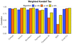
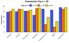
Figure 5: Weighted Kedall’s Tau and Intersection between the Top $50$ nodes in the exact ranking and the approximated ones (with parameters $\varepsilon=0.1,c=2$) for the prefix-foremost-temporal betweenness

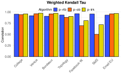
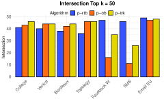
Figure 6: Weighted Kedall’s Tau and Intersection between the Top $50$ nodes in the exact ranking and the approximated ones (with parameters $\varepsilon=0.07,c=3$) for the prefix-foremost-temporal betweenness

E.2 Fixed sample size algorithms

In this section we show the results of the experiments for the fixed sample-size algorithms. For each temporal optimality criteria we use the result of Theorem 14 as an upper bound on the sample size. We point out that such result holds only for the shortest-temporal betweenness. However, from our experiments we can see that using this bound as an heuristic for the other types of temporal-betweenness gives good estimations as well.

Running times.

Figures 7-8-9 show the running times of the algorithms for all the temporal path optimality criteria and values of $\varepsilon\in\{0.05,0.07,0.1\}$ and $\delta=0.1$. As expected, rtb does not scale as the size of the network increases, while ob, and trk have similar performances and are always preferable to rtb.

Estimation error.

In Figures 11-11-12, for each algorithm, we show the average mean squared error of the estimated betweenness values. There is no clear winner between our approaches, rtb gives better betweenness vales estimations on networks with low connectivity rate i.e., Facebook wall and SMS, while ob, and trk  perform equally better than rtb on the remaining temporal graphs. This result gives us a rule of thumb on which approximation approach to choose: given a temporal graph $\mathcal{G}$, first we compute $\zeta(\mathcal{G})$, if its temporal connectivity rate is low, we may run rtb (or the other algorithms using a bigger sample size), otherwise we run ob, or trk.

Shortest-temporal betweenness

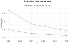
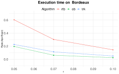
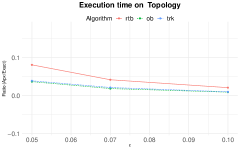
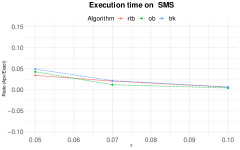
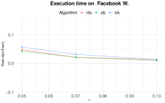
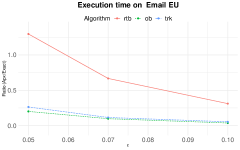
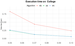
Figure 7: Comparison of the running times between the algorithms for the shortest-temporal betweenness estimation.

Shortest-foremost-temporal betweenness

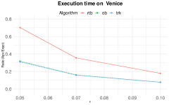
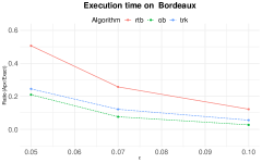
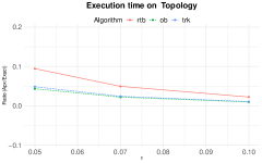
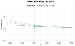
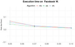
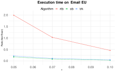
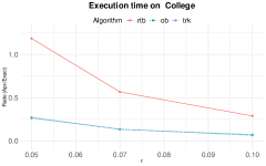
Figure 8: Comparison of the running times between the algorithms for the shortest-foremost-temporal betweenness estimation.

Prefix-foremost-temporal betweenness

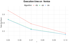
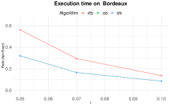
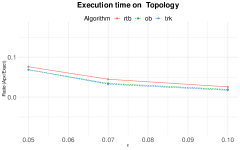
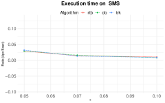
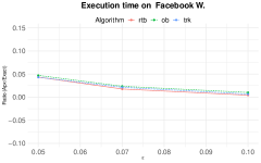
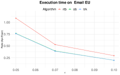
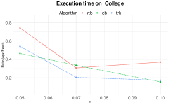
Figure 9: Comparison of the running times between the algorithms for the prefix-foremost-temporal betweenness estimation.

Shortest-temporal betweenness

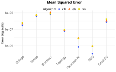
(a) $\varepsilon=0.1$

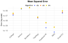
(b) $\varepsilon=0.07$

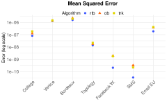
(c) $\varepsilon=0.05$

Figure 10: Algorithms’s mean squared errors for the shortest-temporal betweenness estimation.

Shortest-foremost-temporal betweenness

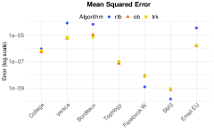
(d) $\varepsilon=0.1$

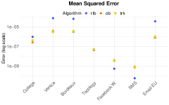
(e) $\varepsilon=0.07$

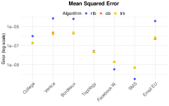
(f) $\varepsilon=0.05$

Figure 11: Algorithms’s mean squared errors for the shortest-foremost-temporal betweenness estimation.

Prefix-foremost-temporal betweenness

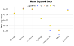
(a) $\varepsilon=0.1$

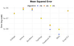
(b) $\varepsilon=0.07$

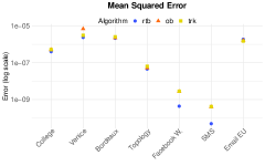
(c) $\varepsilon=0.05$

Figure 12: Algorithms’s mean squared errors for the prefix-temporal betweenness estimation.

Appendix F Pseudo codes

Data: $\mathcal{B},\mathcal{B}_{1},\mathcal{B}_{2}$, node $u\in V$, and real value $h_{u}$

1

2$v=\mathcal{B}_{2}[u]$

3$v_{1}=v+h_{u}^{2}$

4if $v_{1}\notin\mathcal{B}$  then

5       $\mathcal{B}[v_{1}]=1$

6 else

7       $\mathcal{B}[v_{1}]=\mathcal{B}[v_{1}]+1$

8 if $v_{1}>0$ and $\mathcal{B}[v]\geq 1$  then

9      

10      $\mathcal{B}[v]=\mathcal{B}[v]-1$

11if $v>0$ and $\mathcal{B}[v]=0$  then

12      

13      removeKey $\mathcal{B}[v]$

14

15$\mathcal{B}_{1}[v]=\mathcal{B}_{1}[v]+h_{u}$

16$\mathcal{B}_{2}[v]=\mathcal{B}_{2}[v]+h_{u}^{2}$

Algorithm 2 UpdateValues

1

Data: Temporal graph $\mathcal{G},\varepsilon$, sample size $s$, and effective shortest temporal diameters’s threshold $\tau$

Result: $D,D_{\tau},\zeta_{\mathcal{G}},\texttt{AvgDist}$

2

$dd=[0,0,\dots,0];R=[0,0,\dots,0]$

  // Arrays of $n$ zeros

3

4$\texttt{acc}=0;\texttt{MaxDistance}=0;\texttt{AvgDist}=0;D,D_{\tau}=-1$

5for $s\in S$ do

6       for $v\in V$ do

7             $dist_{v}=-1$

8      for $(u,v,t)\in\mathcal{E}$ do

9             $dist_{v,t}=-1$

10      $dist_{s}=0;dist_{s,0}=0$

11      $dd[0]=dd[0]+1$

12      $Q=\text{empty queue};Q.enqueue((s,0))$

13      while $!Q.empty()$ do

14             $(v,t)=Q.dequeue()$

15            for $(w,t^{\prime})\in N^{out}(v,t)$ do

16                   if $dist_{w,t^{\prime}}=-1$ then

17                        

18                        $dist_{w,t^{\prime}}=dist_{v,t}+1$

19                        if $dist_{w}=-1$ then

20                              

21                              $dist_{w}=dist_{v,t}+1$

22                              $dd[dist_{w}]=dd[dist_{w}]+1$

23                              $\texttt{MaxDistance}=\max\left(\texttt{MaxDistance},dist_{w}\right)$

24                        $Q.enqueue((w,t^{\prime}))$

25                  

26            

27      

28

29for $h\in\{0,\dots,\texttt{MaxDistance}\}$ do

30      

31      $\texttt{acc}=\texttt{acc}+dd[h]$

32      $R[h]=\frac{n}{s}\cdot\texttt{acc}$

33for $h\in\{0,\dots,\texttt{MaxDistance}\}$ do

34      

      $\texttt{AvgDist}=(R[h]-R[h-1])\cdot h$

        // $R[-1]$ threaded as 0 when $h=0$

35      

36

37$\texttt{AvgDist}=\texttt{AvgDist}/R[\texttt{MaxDistance}]$

38$D_{\tau}=\min_{h}\left(r:\frac{R[h]}{R[\texttt{MaxDistance}]}\geq\tau\right)$

39$\zeta_{\mathcal{G}}=\frac{R[\texttt{MaxDistance}]}{n(n-1)}$

40return $\texttt{MaxDistance},D_{\tau},\zeta_{\mathcal{G}},\texttt{AvgDist}$

Algorithm 3 Shortest temporal (effective) diameter approximation

References

- [1] George B. Mertzios, Othon Michail, and Paul G. Spirakis. Temporal network optimization subject to connectivity constraints. Algorithmica, 2019.
- [2] John Kit Tang, Mirco Musolesi, Cecilia Mascolo, Vito Latora, and Vincenzo Nicosia. Analysing information flows and key mediators through temporal centrality metrics. In Proceedings of the 3rd Workshop on Social Network Systems, Paris, France, April 13, 2010, 2010.
- [3] Elizabeth M. Daly and Mads Haahr. Social network analysis for routing in disconnected delay-tolerant manets. In Proceedings of the 8th ACM Interational Symposium on Mobile Ad Hoc Networking and Computing, MobiHoc 2007, Montreal, Quebec, Canada, September 9-14, 2007, 2007.
- [4] Özgür Simsek and Andrew G. Barto. Skill characterization based on betweenness. In Advances in Neural Information Processing Systems 21, Proceedings of the Twenty-Second Annual Conference on Neural Information Processing Systems, Vancouver, British Columbia, Canada, December 8-11, 2008, 2008.
- [5] Martijn P van den Heuvel, René CW Mandl, Cornelis J Stam, René S Kahn, and Hilleke E Hulshoff Pol. Aberrant frontal and temporal complex network structure in schizophrenia: a graph theoretical analysis. Journal of Neuroscience, 2010.
- [6] Ulrik Brandes. A faster algorithm for betweenness centrality. Journal of mathematical sociology, 2001.
- [7] Amir Abboud, Fabrizio Grandoni, and Virginia Vassilevska Williams. Subcubic equivalences between graph centrality problems, APSP and diameter. In Proceedings of the Twenty-Sixth Annual ACM-SIAM Symposium on Discrete Algorithms, SODA 2015, San Diego, CA, USA, January 4-6, 2015, 2015.
- [8] Michele Borassi, Pierluigi Crescenzi, and Michel Habib. Into the square: On the complexity of some quadratic-time solvable problems. In Proceedings of the 16th Italian Conference on Theoretical Computer Science, ICTCS 2015, Firenze, Italy, September 9-11, 2015, 2015.
- [9] Sebastian Buß, Hendrik Molter, Rolf Niedermeier, and Maciej Rymar. Algorithmic aspects of temporal betweenness. In KDD ’20: The 26th ACM SIGKDD Conference on Knowledge Discovery and Data Mining, Virtual Event, CA, USA, August 23-27, 2020. ACM, 2020.
- [10] Maciej Rymar, Hendrik Molter, André Nichterlein, and Rolf Niedermeier. Towards classifying the polynomial-time solvability of temporal betweenness centrality. In Graph-Theoretic Concepts in Computer Science - 47th International Workshop, WG 2021, Warsaw, Poland, June 23-25, 2021, Revised Selected Papers, Lecture Notes in Computer Science. Springer, 2021.
- [11] Diego Santoro and Ilie Sarpe. ONBRA: rigorous estimation of the temporal betweenness centrality in temporal networks. CoRR, 2022.
- [12] Matteo Riondato and Evgenios M. Kornaropoulos. Fast approximation of betweenness centrality through sampling. In Seventh ACM International Conference on Web Search and Data Mining, WSDM 2014, New York, NY, USA, February 24-28, 2014. ACM, 2014.
- [13] Michele Borassi and Emanuele Natale. KADABRA is an adaptive algorithm for betweenness via random approximation. ACM J. Exp. Algorithmics, 2019.
- [14] Ulrik Brandes and Christian Pich. Centrality estimation in large networks. Int. J. Bifurc. Chaos, 2007.
- [15] David A. Bader, Shiva Kintali, Kamesh Madduri, and Milena Mihail. Approximating betweenness centrality. In Algorithms and Models for the Web-Graph, 5th International Workshop, WAW 2007, San Diego, CA, USA, December 11-12, 2007, Proceedings, Lecture Notes in Computer Science. Springer, 2007.
- [16] Matteo Riondato and Eli Upfal. ABRA: approximating betweenness centrality in static and dynamic graphs with rademacher averages. ACM Trans. Knowl. Discov. Data, 2018.
- [17] Cyrus Cousins, Chloe Wohlgemuth, and Matteo Riondato. Bavarian: Betweenness centrality approximation with variance-aware rademacher averages. In KDD ’21: The 27th ACM SIGKDD Conference on Knowledge Discovery and Data Mining, Virtual Event, Singapore, August 14-18, 2021, 2021.
- [18] Leonardo Pellegrina and Fabio Vandin. SILVAN: estimating betweenness centralities with progressive sampling and non-uniform rademacher bounds. 2021.
- [19] Ioanna Tsalouchidou, Ricardo Baeza-Yates, Francesco Bonchi, Kewen Liao, and Timos Sellis. Temporal betweenness centrality in dynamic graphs. Int. J. Data Sci. Anal., 2020.
- [20] Binh-Minh Bui-Xuan, Afonso Ferreira, and Aubin Jarry. Computing shortest, fastest, and foremost journeys in dynamic networks. Int. J. Found. Comput. Sci., 2003.
- [21] Foster J. Provost, David D. Jensen, and Tim Oates. Efficient progressive sampling. In Proceedings of the Fifth ACM SIGKDD International Conference on Knowledge Discovery and Data Mining, San Diego, CA, USA, August 15-18, 1999. ACM, 1999.
- [22] Wassily Hoeffding. Probability inequalities for sums of bounded random variables. Journal of the American statistical association, 1963.
- [23] Othon Michail. An introduction to temporal graphs: An algorithmic perspective. 2016.
- [24] Riko Jacob, Dirk Koschützki, Katharina Anna Lehmann, Leon Peeters, and Dagmar Tenfelde-Podehl. Algorithms for centrality indices. In Network Analysis: Methodological Foundations [outcome of a Dagstuhl seminar, 13-16 April 2004], Lecture Notes in Computer Science. Springer, 2004.
- [25] Richard J. Lipton and Jeffrey F. Naughton. Estimating the size of generalized transitive closures. In Peter M. G. Apers and Gio Wiederhold, editors, Proceedings of the Fifteenth International Conference on Very Large Data Bases, August 22-25, 1989, Amsterdam, The Netherlands, 1989.
- [26] Andreas Maurer and Massimiliano Pontil. Empirical bernstein bounds and sample-variance penalization. In COLT 2009 - The 22nd Conference on Learning Theory, Montreal, Quebec, Canada, June 18-21, 2009, 2009.
- [27] Boucheron, Stéphane, Bousquet, Olivier, and Lugosi, Gábor. Theory of classification: a survey of some recent advances. ESAIM: PS, 2005.
- [28] R. Kujala, C. Weckström, R. Darst, M. Madlenocić, and J. Saramäki. A collection of public transport network data sets for 25 cities. Sci. Data, 2018.
- [29] Jure Leskovec and Andrej Krevl. SNAP Datasets: Stanford large network dataset collection. http://snap.stanford.edu/data, last checked on March 25, 2023.
- [30] J. Kunegis. The KONECT Project. http://konect.cc, last checked on March 25, 2023.
- [31] Ryan A. Rossi and Nesreen K. Ahmed. Network repository. https://networkrepository.com, last checked on March 25, 2023.