POD-ROMs for incompressible flows including snapshots of the temporal derivative of the full order solution: Error bounds for the pressure

Abstract

Reduced order methods (ROMs) for the incompressible Navier–Stokes equations, based on proper orthogonal decomposition (POD), are studied that include snapshots which approach the temporal derivative of the velocity from a full order mixed finite element method (FOM). In addition, the set of snapshots contains the mean velocity of the FOM. Both the FOM and the POD-ROM are equipped with a grad-div stabilization. A velocity error analysis for this method can be found already in the literature. The present paper studies two different procedures to compute approximations to the pressure and proves error bounds for the pressure that are independent of inverse powers of the viscosity. Numerical studies support the analytic results and compare both methods.

AMS subject classifications. 65M12, 65M15, 65M60.
Keywords. incompressible Navier–Stokes equations, proper orthogonal decomposition (POD), reduced order models (ROMs), snapshots of the temporal derivative, grad-div stabilization, robust pointwise in time estimates, pressure bounds

1 Introduction

It is sometimes necessary to compute numerical approximations of solutions of partial differential equations very fast without requiring the highest accuracy. An example is the solution of optimal control problems, which needs in each iteration the solution of a time-dependent partial differential equation with only slightly changed data. A popular approach for performing highly efficient simulations consists in using so-called reduced order models (ROMs). These models utilize a Galerkin approach and the corresponding basis functions are extracted from one accurate numerical solution, which is called in this context the full order model (FOM).

This paper studies incompressible flow problems that are modeled by the incompressible Navier–Stokes equations

$$\begin{array}[]{rcll}\partial_{t}\boldsymbol{u}-\nu\Delta\boldsymbol{u}+(\boldsymbol{u}\cdot\nabla)\boldsymbol{u}+\nabla p&=&\boldsymbol{f}&\text{in }\ (0,T]\times\Omega,\\ \nabla\cdot\boldsymbol{u}&=&0&\text{in }\ (0,T]\times\Omega,\end{array}$$ (1)

in a bounded domain $\Omega\subset{\mathbb{R}}^{d}$, $d\in\{2,3\}$. The boundary of $\Omega$ is assumed to be polyhedral and Lipschitz. In (1), $\boldsymbol{u}$ denotes the velocity field, $p$ the kinematic pressure, $\nu>0$ the kinematic viscosity coefficient, and $\boldsymbol{f}$ represents the accelerations due to external body forces acting on the fluid. The Navier–Stokes equations (1) have to be complemented with an initial condition $\boldsymbol{u}(0,\boldsymbol{x})=\boldsymbol{u}^{0}(\boldsymbol{x})$ and with boundary conditions. For simplicity, we only consider the case of homogeneous Dirichlet boundary conditions $\boldsymbol{u}=\boldsymbol{0}$ on $[0,T]\times\partial\Omega$.

The most popular approach for computing basis functions for ROMs is probably the use of the proper orthogonal decomposition (POD), which will be also considered here. The complete method is often called POD-ROM. In the past few years there has been a tremendous progress in the numerical analysis of POD-ROM methods, e.g., see [22, 16, 20, 18, 21, 7, 15, 12, 13, 11]. In [11], we introduced a POD-ROM model based on a set of snapshots including the mean value of the velocity at different time instants together with approximations to the velocity time derivative at different times. Including grad-div stabilization, both in the snapshots computation and the POD-ROM method, we were able to prove error bounds for the velocity that are convection-robust, i.e., the constants in the error bounds are independent of inverse powers of the viscosity.

There are applications that require the pressure solution for computing quantities of interest, e.g., lift or drag coefficients at bodies in the flow field. In other applications, the pressure is even more important than the velocity, e.g., the pressure gradient is the most important biomarker for detecting stenoses in blood vessels. Using in the FOM a pair of finite element spaces that satisfies a discrete inf-sup condition, then the basis functions from the POD are discretely divergence-free. Consequently, the POD-ROM, as a Galerkin method, does not contain the pressure. This situation was considered in [11].

The goal of this paper consists in analyzing two algorithms for computing a reduced order pressure. Both algorithms use a set of velocity snapshots that are based on approximations of the temporal derivative of the FOM velocity and on pressure snapshots that are solutions of the FOM. The first algorithm is the supremizer enrichment algorithm from [21]. In the present paper, the analysis of [21] is extended from a ROM that uses standard FOM velocity snapshots to a ROM that utilizes the above mentioned approximations of the temporal derivative of the velocity. The second algorithm is the so-called stabilization-motivated POD-ROM proposed in [6]. This method is already analyzed in [7] and the present paper aims to improve this analysis in several aspects. First, we avoid the strong restriction $h\leq C\Delta t$, where $\Delta t$ and $h$ are the time step and spatial mesh diameter, respectively. Second, differently to [7], we use the same procedure to compute a POD-ROM pressure in two and three spatial dimensions. Note that in [7] a so-called truncation of the velocity approximation is applied in the nonlinear convective term to compute the reduced order pressure. Third, in contrast to [7], where only a first order convergence for the considered norm could be proved, our analysis shows for the same norm an order that is induced from the pair of mixed finite element spaces that were used for performing the FOM simulation. And finally, again in contrast to [7], the constant in the derived error bound does not blow up if the viscosity coefficient tends to zero.

Numerical studies will support the analytic results. These studies will also provide an initial comparison of the supremizer enrichment and the stabilization-motivated pressure ROMs.

The paper is organized as follows. Section 2 introduces some notations, the considered finite element spaces, recalls some inequalities used in the numerical analysis, and presents the FOM. In Section 3 the error estimates for the POD-ROM velocity from [11] are recalled and a few new estimates for velocity terms are proved. The numerical analysis for the pressure ROMs is presented in Section 4 and Section 5 contains the numerical studies. Finally, a summary of the results and an outlook is given in Section 6.

2 Finite Element Spaces and the FOM

Standard symbols will be used for Lebesgue and Sobolev spaces, with the usual convention that $W^{s,2}(\Omega)=H^{s}(\Omega)$, $s\geq 1$. The inner product in $L^{2}(\Omega)^{d}$, $d\geq 1$, is denoted by $(\cdot,\cdot)$. In the sequel we denote $L_{0}^{2}(\Omega)=\{q\in L^{2}(\Omega)\ \mid\ (q,1)=0\}$. Let us recall the Poincaré inequality,

$$\|\boldsymbol{v}\|_{0}\leq C_{p}\|\nabla\boldsymbol{v}\|_{0}\quad\forall\ \boldsymbol{v}\in H^{1}_{0}(\Omega)^{d},$$ (2)

and the estimate of the divergence of a velocity field by its gradient, see [14, Remark 3.35],

$$\|\nabla\cdot\boldsymbol{v}\|_{0}\leq\|\nabla\boldsymbol{v}\|_{0}\quad\forall\ \boldsymbol{v}\in H^{1}_{0}(\Omega)^{d}.$$ (3)

The following Sobolev embeddings [1] will be used in the analysis: For $q\in[1,\infty)$, there exists a constant $C=C(\Omega,q)$ such that

$$\|v\|_{L^{q^{\prime}}}\leq C\|v\|_{W^{s,q}},\,\,\quad\frac{1}{q^{\prime}}\geq\frac{1}{q}-\frac{s}{d}>0,\quad q<\infty,\quad v\in W^{s,q}(\Omega)^{d}.$$ (4)

Generic constants independent of inverse powers of the viscosity and the mesh width are denoted by $C$, $C_{0}$ and similar symbols.

Let us denote by $\{\mathcal{T}_{h}\}=\{(K_{j},\phi_{j}^{h})_{j\in J_{h}}\}$, $h>0$, a family of partitions of $\overline{\Omega}$, where $h$ is the maximum diameter of the mesh cells $K_{j}\in\mathcal{T}_{h}$ and $\phi_{j}^{h}$ are the mappings from the reference simplex $K_{0}$ onto $K_{j}$. We assume that the family of partitions is shape-regular and quasi-uniform. On $\mathcal{T}_{h}$, the following finite element spaces are defined

$$Y_{h}^{l} = \left\{v_{h}\in C^{0}(\overline{\Omega})\ \mid\ {v_{h}}_{\mid_{K}}\in{\mathbb{P}}_{l}(K),\ \forall\ K\in\mathcal{T}_{h}\right\},\ l\geq 1,\quad{\boldsymbol{Y}}_{h}^{l}=\left(Y_{h}^{l}\right)^{d},$$

$${\boldsymbol{X}}_{h}^{l} = {\boldsymbol{Y}}_{h}^{l}\cap H_{0}^{1}(\Omega)^{d},$$

$$Q_{h}^{l} = Y_{h}^{l}\cap L_{0}^{2}(\Omega),$$

$${\boldsymbol{V}}_{h}^{l} = {\boldsymbol{X}}_{h}^{l}\cap\left\{{\boldsymbol{v}}_{h}\in H_{0}^{1}(\Omega)^{d}\ \mid\ (\nabla\cdot{\boldsymbol{v}}_{h},q_{h})=0\ \forall\ q_{h}\in Q_{h}^{l-1}\right\},\quad l\geq 2.$$

Hence, ${\boldsymbol{V}}_{h}^{l}$ is the space of discretely divergence-free functions.

The Lagrangian interpolant in ${\boldsymbol{X}}_{h}^{l}$ is denoted by $I_{h}(\cdot)$. It is well known, e.g., see [4], that there exists a constant $C>0$ such that for every $K\in{\cal T}_{h}$

$$\left\|\boldsymbol{u}-I_{h}(\boldsymbol{u})\right\|_{0,K}+h\left\|\nabla(\boldsymbol{u}-I_{h}(\boldsymbol{u}))\right\|_{0,K}+h^{2}\|\Delta(\boldsymbol{u}-I_{h}(\boldsymbol{u}))\|_{0,K}\leq C\|\boldsymbol{u}\|_{l+1,K}h^{l+1}.$$ (5)

The inverse inequality

$$|v_{h}|_{W^{m,p}(K)}\leq c_{\mathrm{inv}}h_{K}^{n-m-d\left(\frac{1}{q}-\frac{1}{p}\right)}\quad|v_{h}|_{W^{n,q}(K)}\quad\forall\ v_{h}\in Y_{h}^{l},$$ (6)

holds, with $0\leq n\leq m\leq 1$, $1\leq q\leq p\leq\infty$, and $h_{K}$ being the diameter of $K\in\mathcal{T}_{h}$, because the family of partitions is quasi-uniform, e.g., see [8, Theorem 3.2.6]. Define $h=\max_{K\in{\cal T}_{h}}h_{K}$.

In this paper, we consider Taylor–Hood pairs of finite element spaces [5, 24], i.e., pairs of the form $({\boldsymbol{X}}_{h}^{l},Q_{h}^{l-1})$, $l\geq 2$. These pairs satisfy a discrete inf-sup condition, see [2, 3], that is, there is a constant $\beta_{\rm is}>0$ independent of $h$ such that

$$\inf_{q_{h}\in Q_{h}^{l-1}}\sup_{\boldsymbol{v}_{h}\in{\boldsymbol{X}}_{h}^{l}}\frac{(\nabla\cdot\boldsymbol{v}_{h},q_{h})}{\|\nabla\boldsymbol{v}_{h}\|_{0}\|q_{h}\|_{0}}\geq\beta_{\rm{is}}.$$ (7)

Taylor–Hood pairs, in particular for $l=2$, are probably the most popular pairs of inf-sup stable finite element spaces.

Let ${\boldsymbol{V}}$ be the space of functions in $H_{0}^{1}(\Omega)^{d}$ with $\nabla\cdot\boldsymbol{u}=0$. The following modified Stokes projection $\boldsymbol{s}_{h}^{m}\ :\ {\boldsymbol{V}}\rightarrow{\boldsymbol{V}}_{h}^{l}$ was introduced in [9] and is defined by

$$(\nabla\boldsymbol{s}_{h}^{m},\nabla\boldsymbol{\varphi}_{h})=(\nabla\boldsymbol{u},\nabla\boldsymbol{\varphi}_{h}),\quad\forall\ \boldsymbol{\varphi}_{h}\in{\boldsymbol{V}_{h}^{l}}.$$ (8)

This projection satisfies the following error bound, see [9],

$$\|\boldsymbol{u}-\boldsymbol{s}_{h}^{m}\|_{0}+h\|\boldsymbol{u}-\boldsymbol{s}_{h}^{m}\|_{1}\leq C\|\boldsymbol{u}\|_{j}h^{j},\quad 1\leq j\leq l+1.$$ (9)

As FOM, we use a Galerkin method with grad-div stabilization. The continuous-in-time method reads as follows: Find $(\boldsymbol{u}_{h},p_{h})\in{\boldsymbol{X}}_{h}^{l}\times Q_{h}^{l-1}$ such that

$$\begin{array}[]{rcll}\left(\partial_{t}\boldsymbol{u},\boldsymbol{v}_{h}\right)+\nu(\nabla\boldsymbol{u}_{h},\nabla\boldsymbol{v}_{h})+b(\boldsymbol{u}_{h},\boldsymbol{u}_{h},\boldsymbol{v}_{h})\\ -(\nabla\cdot\boldsymbol{v}_{h},p_{h})+\mu(\nabla\cdot\boldsymbol{u}_{h},\nabla\cdot\boldsymbol{v}_{h})&=&({\boldsymbol{f}},\boldsymbol{v}_{h})&\forall\ \boldsymbol{v}_{h}\in{\boldsymbol{X}}_{h}^{l},\\ (\nabla\cdot\boldsymbol{u}_{h},q_{h})&=&0&\forall\ q_{h}\in Q_{h}^{l-1},\end{array}$$

where $\mu$ is the positive grad-div stabilization parameter and

$$b(\boldsymbol{u},\boldsymbol{v},\boldsymbol{w})=((\boldsymbol{u}\cdot\nabla)\boldsymbol{v},\boldsymbol{w})+\frac{1}{2}((\nabla\cdot\boldsymbol{u})\boldsymbol{v},\boldsymbol{w}).$$

The pressure drops out if the problem is considered for functions from the discretely divergence-free space $\boldsymbol{V}_{h}^{l}$, since $\boldsymbol{u}_{h}\in\boldsymbol{V}_{h}^{l}$ satisfies

$$\left(\partial_{t}\boldsymbol{u}_{h},\boldsymbol{v}_{h}\right)+\nu(\nabla\boldsymbol{u}_{h},\nabla\boldsymbol{v}_{h})+b(\boldsymbol{u}_{h},\boldsymbol{u}_{h},\boldsymbol{v}_{h})$$

$$+\mu(\nabla\cdot\boldsymbol{u}_{h},\nabla\cdot\boldsymbol{v}_{h}) = ({\boldsymbol{f}},\boldsymbol{v}_{h})\quad\forall\ \boldsymbol{v}_{h}\in{\boldsymbol{V}}_{h}^{l}.$$ (10)

For this method the following bound holds, see [9] for the first term and the explanation in [11] for the second term,

$$\|\boldsymbol{u}(t,\cdot)-\boldsymbol{u}_{h}(t,\cdot)\|_{0}+h\|\boldsymbol{u}(t,\cdot)-\boldsymbol{u}_{h}(t,\cdot)\|_{1}\leq C(\boldsymbol{u},p,l+1)h^{l},\quad t\in(0,T],$$ (11)

where the constant $C(\boldsymbol{u},p,l+1)$ does not explicitly depend on inverse powers of $\nu$. To bound the error in the pressure, arguing as in [9], and using results in [10], one can prove

$$\left(\sum_{j=1}^{n}\Delta t\left\|p^{j}-p_{h}^{j}\right\|_{0}^{2}\right)^{1/2}\leq C_{\rm press}(\boldsymbol{u},p,l+1)h^{l-1/2}.$$ (12)

3 Velocity POD-ROMs

This section describes briefly the velocity POD-ROMs that were investigated in [11] and summarizes the error estimates derived in this paper.

3.1 The General Method

Let $M\in\mathbb{N}$ be a positive integer and set $\Delta t=T/M$, i.e., the time instants are given by $t_{j}=j\Delta t$, $j=0,\ldots,M$. For simplicity of presentation, let $\boldsymbol{u}_{h}^{j}=\boldsymbol{u}_{h}(t_{j},\cdot)$, $p_{h}^{j}=p_{h}(t_{j},\cdot)$ denote the FOM approximation of the velocity at time instant $t_{j}$ and $\partial_{t}\boldsymbol{u}_{h}^{j}=\partial_{t}\boldsymbol{u}_{h}(t_{j},\cdot)$ the approximation of the temporal derivative (e.g., see [11, Remark 2.1] on the computation of time derivatives). The mean value of the velocity snapshots is defined by $\overline{\boldsymbol{u}}_{h}=\frac{1}{N}\sum_{j=0}^{M}\boldsymbol{u}_{h}^{j}$ with $N=M+1$. Then, the following space, which is based on data from the FOM simulation, is defined

$${\mathcal{\boldsymbol{U}}}=\mbox{span}\left\{\sqrt{N}\overline{\boldsymbol{u}}_{h},\tau\partial_{t}\boldsymbol{u}_{h}^{1},\ldots,\tau\partial_{t}\boldsymbol{u}_{h}^{M}\right\}=\mbox{span}\left\{\boldsymbol{y}_{h}^{1},\boldsymbol{y}_{h}^{2},\ldots,\boldsymbol{y}_{h}^{N}\right\}.$$ (13)

The factor $\tau$ in front of the temporal derivatives is a time scale. Its introduction aims to make the vectors $\boldsymbol{y}_{h}^{j}$, $j=1,\ldots,N$, dimensionally correct, i.e., all vectors possess the physical unit $\nicefrac{\mathrm{m}}{\mathrm{s}}$. The dimension of $\mathcal{\boldsymbol{U}}$ is denoted by $d_{v}$.

Notice that by taking derivatives with respect to time in the second equation in (2) it follows that $\partial_{t}\boldsymbol{u}_{h}^{j}$ is discretely divergence-free, i.e., $\partial_{t}\boldsymbol{u}_{h}^{j}\in\boldsymbol{V}_{h,l}$ for all $j=1,\ldots,M$, so that $\mathcal{\boldsymbol{U}}\subset\boldsymbol{V}_{h,l}$.

Let the space $\mathcal{\boldsymbol{U}}$ be equipped with an inner product, denoted by $(\cdot,\cdot)_{X}$. For the Navier–Stokes equations, this might be the product from $L^{2}(\Omega)^{d}$ or from $H_{0}^{1}(\Omega)^{d\times d}$. Both cases will be considered in the present paper. Then, the first step of the POD approach consists in defining the correlation matrix $K^{\mathrm{v}}=((k_{i,j}^{\mathrm{v}}))\in{\mathbb{R}}^{N\times N}$ with the entries

$$k_{i,j}^{\mathrm{v}}=\frac{1}{N}\left(\boldsymbol{y}_{h}^{i},\boldsymbol{y}_{h}^{j}\right)_{X},\quad i,j=1,\ldots,N.$$

Denote by $\lambda_{1}\geq\lambda_{2},\ldots\geq\lambda_{d_{v}}>0$ the positive eigenvalues of $K^{\mathrm{v}}$ and by $\boldsymbol{v}_{1},\ldots,\boldsymbol{v}_{d_{v}}\in{\mathbb{R}}^{N}$ associated eigenvectors with Euclidean norm $1$. Then, the POD basis functions of $\mathcal{\boldsymbol{U}}$, which are orthonormal, are defined by

$$\boldsymbol{\varphi}_{k}=\frac{1}{\sqrt{N}}\frac{1}{\sqrt{\lambda_{k}}}\sum_{j=1}^{N}v_{k}^{j}\boldsymbol{y}_{h}^{j},$$

with $v_{k}^{j}$ being the $j$-th component of $\boldsymbol{v}_{k}$. The following representation of the error was derived in [19, Proposition 1]

$$\frac{1}{N}\sum_{j=1}^{N}\left\|\boldsymbol{y}_{h}^{j}-\sum_{k=1}^{r}\left(\boldsymbol{y}_{h}^{j},\boldsymbol{\varphi}_{k}\right)_{X}\boldsymbol{\varphi}_{k}\right\|_{X}^{2}=\sum_{k=r+1}^{d_{v}}\lambda_{k}.$$

Inserting the functions from (13) yields

$$\left\|\overline{\boldsymbol{u}}_{h}-\sum_{k=1}^{r}\left(\overline{\boldsymbol{u}}_{h},\boldsymbol{\varphi}_{k}\right)_{X}\boldsymbol{\varphi}_{k}\right\|_{X}^{2}$$

$$+\frac{\tau^{2}}{M+1}\sum_{j=1}^{M}\left\|\partial_{t}\boldsymbol{u}_{h}^{j}-\sum_{k=1}^{r}\left(\partial_{t}\boldsymbol{u}_{h}^{j},\boldsymbol{\varphi}_{k}\right)_{X}\boldsymbol{\varphi}_{k}\right\|_{X}^{2} = \sum_{k=r+1}^{d_{v}}\lambda_{k}.$$ (14)

The stiffness matrix of the POD basis is defined by $S^{\mathrm{v}}=((s_{i,j}^{\mathrm{v}}))\in{\mathbb{R}}^{d_{v}\times d_{v}}$, where $s_{i,j}^{\mathrm{v}}=(\nabla\boldsymbol{\varphi}_{j},\nabla\boldsymbol{\varphi}_{i})_{X}$. In the case $X=L^{2}(\Omega)^{d}$, the following estimate was shown in [19, Lemma 2]:

$$\|\nabla\boldsymbol{v}\|_{0}\leq\sqrt{\|S^{\mathrm{v}}\|_{2}}\|\boldsymbol{v}\|_{0}\quad\forall\ \boldsymbol{v}\in{\mathcal{\boldsymbol{U}}}.$$ (15)

We will denote the space spanned by the first $r$ POD basis functions by

$${\mathcal{\boldsymbol{U}}}^{r}=\mbox{span}\left\{\boldsymbol{\varphi}_{1},\boldsymbol{\varphi}_{2},\ldots,\boldsymbol{\varphi}_{r}\right\},\quad 1\leq r\leq d_{v},$$

and by $P_{r}^{\mathrm{v}}\ :\ {\boldsymbol{X}}_{h}^{l}\to{\mathcal{\boldsymbol{U}}}^{r}$, the $X$-orthogonal projection onto ${\mathcal{\boldsymbol{U}}}^{r}$.

In [11, (3.11)], we proved for any Banach space $Y$ defined on $\Omega$ the estimate

$$\max_{0\leq k\leq N}\|\boldsymbol{z}^{k}\|_{Y}^{2}\leq{3}\|\overline{\boldsymbol{z}}\|_{Y}^{2}+\frac{12T^{2}}{M}\sum_{n=1}^{M}\|\partial_{t}\boldsymbol{z}^{n}\|_{Y}^{2}+\frac{16T}{3}(\Delta t)^{2}\int_{0}^{T}\|\partial_{tt}\boldsymbol{z}\|_{Y}^{2}\ ds,$$ (16)

provided that $\boldsymbol{z}\in H^{2}(0,T;Y)$. Applying (16) to $\boldsymbol{u}_{h}^{n}-P_{r}^{\mathrm{v}}\boldsymbol{u}_{h}^{n}$ yields

$$\max_{0\leq n\leq M}\|\boldsymbol{u}_{h}^{n}-P_{r}^{\mathrm{v}}\boldsymbol{u}_{h}^{n}\|_{Y}^{2} \leq 3\|\overline{\boldsymbol{u}_{h}^{n}-P_{r}^{\mathrm{v}}\boldsymbol{u}_{h}^{n}}\|_{Y}^{2}+\frac{12T^{2}}{M}\sum_{n=1}^{M}\|\partial_{t}\boldsymbol{u}_{h}^{n}-P_{r}^{\mathrm{v}}\partial_{t}\boldsymbol{u}_{h}^{n}\|_{Y}^{2}$$ (17)

$$\quad+\frac{16T}{3}(\Delta t)^{2}\int_{0}^{T}\|\partial_{tt}\boldsymbol{u}_{h}-P_{r}^{\mathrm{v}}\partial_{tt}\boldsymbol{u}_{h}^{n}\|_{Y}^{2}\ ds.$$

Let $Y=X$, the space that is connected to the projection $P_{r}^{\mathrm{v}}$. Using the $X$-stability of the projection gives

$$\|\partial_{tt}\boldsymbol{u}_{h}-P_{r}^{\mathrm{v}}\partial_{tt}\boldsymbol{u}_{h}\|_{X}^{2}\leq 2\|P_{r}^{\mathrm{v}}\partial_{tt}\boldsymbol{u}_{h}\|_{X}^{2}+2\|\partial_{tt}\boldsymbol{u}_{h}\|_{X}^{2}\leq 4\|\partial_{tt}\boldsymbol{u}_{h}\|_{X}^{2},$$

so that we obtain with (3.1)

$$\max_{0\leq n\leq M}\|\boldsymbol{u}_{h}^{n}-P_{r}^{\mathrm{v}}\boldsymbol{u}_{h}^{n}\|_{X}^{2}\leq C_{X}^{2}=\rho^{2}\sum_{k={r+1}}^{d_{v}}\lambda_{k}+\frac{64}{3}T(\Delta t)^{2}\int_{0}^{T}\|\partial_{tt}\boldsymbol{u}_{h}\|_{X}^{2}\ ds,$$ (18)

where

$$\rho=\max\left\{\sqrt{3},\frac{\sqrt{24}T}{\tau}\right\}.$$ (19)

All explicit constants in the bounds (16)–(19) will immediately be absorbed in generic constants in the following analysis.

Summing over all time steps leads to

$$\frac{1}{M}\sum_{n=1}^{M}\left\|\boldsymbol{u}_{h}^{n}-P_{r}^{\mathrm{v}}\boldsymbol{u}_{h}^{n}\right\|_{X}^{2}\leq C_{X}^{2}.$$ (20)

3.2 Velocity Error Estimate for $X=H_{0}^{1}(\Omega)^{d\times d}$

As usual in the analysis of discretizations of the Navier–Stokes equations, errors for the pressure are bounded by velocity errors, which have been estimated before. The velocity error bounds were derived in [11] and they are provided here for completeness of presentation.

For the sake of concentrating the numerical analysis to the essential points, the grad-div POD-ROM model studied in [11] was equipped with the implicit Euler method as temporal discretization: For $n\geq 1$, find $\boldsymbol{u}_{r}^{n}\in{\mathcal{\boldsymbol{U}}}^{r}$ such that

$$\left(\frac{\boldsymbol{u}_{r}^{n}-\boldsymbol{u}_{r}^{n-1}}{\Delta t},\boldsymbol{\varphi}\right)+\nu(\nabla\boldsymbol{u}_{r}^{n},\nabla\boldsymbol{\varphi})+b\left(\boldsymbol{u}_{r}^{n},\boldsymbol{u}_{r}^{n},\boldsymbol{\varphi}\right)+\mu(\nabla\cdot\boldsymbol{u}_{r}^{n},\nabla\cdot\boldsymbol{\varphi})$$ (21)

$$= (\boldsymbol{f}^{n},\boldsymbol{\varphi})\quad\forall\ \boldsymbol{\varphi}\in{\mathcal{\boldsymbol{U}}}^{r}.$$

Since $\partial_{t}\boldsymbol{u}_{h}^{j}\in\boldsymbol{V}_{h,l}$, it follows that $\boldsymbol{u}_{r}^{n}$ belongs to the space of discretely divergence-free functions. Hence, there is no pressure term in (21) and this equation does not need to be augmented with a requirement on the divergence of the solution.

The velocity error estimates in [11] that we present below are convection-robust, i.e., all constants do not depend on inverse powers of the viscosity. Denoting by $\boldsymbol{e}_{r}^{j}=\boldsymbol{u}_{r}^{j}-P_{r}^{\mathrm{v}}\boldsymbol{u}_{h}^{j}$ the following estimate holds for $j=1,\ldots,M$, see [11, (4.21)],

$$\|\boldsymbol{e}_{r}^{j}\|_{0}^{2}+2\nu\sum_{j=1}^{M}\Delta t\|\nabla\boldsymbol{e}_{r}^{j}\|_{0}^{2}+\mu\sum_{j=1}^{M}\Delta t\|\nabla\cdot\boldsymbol{e}_{r}^{j}\|_{0}^{2}$$ (22)

$$\leq C_{0}\|\boldsymbol{e}_{r}^{0}\|_{0}^{2}+C_{1}\sum_{k=r+1}^{d_{v}}\lambda_{k}+C_{2}(\Delta t)^{2}\int_{0}^{T}\|\nabla\partial_{tt}\boldsymbol{u}_{h}\|_{0}^{2}\ ds.$$

The following estimate is proved in [11, Theorem 4.1].

$$\frac{1}{T}\sum_{j=1}^{M}\Delta t\|\boldsymbol{u}_{r}^{j}-\boldsymbol{u}^{j}\|_{0}^{2} \leq C_{0}\|\boldsymbol{u}_{r}^{0}-\boldsymbol{u}_{h}(0)\|_{0}^{2}+C_{1}\sum_{k=r+1}^{d_{v}}\lambda_{k}+C^{2}(\boldsymbol{u},p,l+1)h^{2l}$$ (23)

$${}+C_{2}(\Delta t)^{2}\int_{0}^{T}\|\nabla(\partial_{tt}\boldsymbol{u}_{h})\|_{0}^{2}\ ds.$$

The term with the second order time derivative can be bounded, see [11, Appendix]. However, a robust bound in the case $X=H_{0}^{1}(\Omega)^{d\times d}$ was obtained only for $l\geq 3$. In addition, in [11, Theorem 4.3], it is shown that the right-hand side of (23) is also an upper bound of pointwise-in-time estimates, that is

$$\max_{0\leq n\leq M}\|\boldsymbol{u}_{r}^{n}-\boldsymbol{u}^{n}\|_{0}^{2} \leq C_{0}\|\boldsymbol{u}_{r}^{0}-\boldsymbol{u}_{h}(0)\|_{0}^{2}+C_{1}\sum_{k=r+1}^{d_{v}}\lambda_{k}+C^{2}(\boldsymbol{u},p,l+1)h^{2l}$$

$$+C_{2}(\Delta t)^{2}\int_{0}^{T}\|\nabla(\partial_{tt}\boldsymbol{u}_{h})\|_{0}^{2}\ ds.$$

3.3 Velocity Error Estimate for $X=L^{2}(\Omega)^{d}$

The following bound can be found in [11, (4.25)]: for $j=1\ldots,M$,

$$\|\boldsymbol{e}_{r}^{j}\|_{0}^{2}+2\nu\sum_{j=1}^{M}\Delta t\|\nabla\boldsymbol{e}_{r}^{j}\|_{0}^{2}+\mu\sum_{j=1}^{M}\Delta t\|\nabla\cdot\boldsymbol{e}_{r}^{j}\|_{0}^{2}$$ (24)

$$\leq C_{0}\|\boldsymbol{e}_{r}^{0}\|_{0}^{2}+(C_{1,1}+C_{1,2}\left\|S^{\mathrm{v}}\right\|_{2})\sum_{k=r+1}^{d_{v}}\lambda_{k}$$

$$+(C_{2,1}+C_{2,2}\left\|S^{\mathrm{v}}\right\|_{2})(\Delta t)^{2}\int_{0}^{T}\|\partial_{tt}\boldsymbol{u}_{h}\|_{0}^{2}\ ds.$$

Then, it is proved in [11, Theorem 4.6] that

$$\frac{1}{T}\sum_{j=1}^{M}\Delta t\|\boldsymbol{u}_{r}^{j}-\boldsymbol{u}^{j}\|_{0}^{2} \leq C_{0}\|\boldsymbol{u}_{r}^{0}-\boldsymbol{u}_{h}(0)\|_{0}^{2}+(C_{1,1}+C_{1,2}\left\|S^{\mathrm{v}}\right\|)\sum_{k=r+1}^{d_{v}}\lambda_{k}$$

$$+C(\boldsymbol{u},p,l+1)h^{2l}$$

$$+(C_{2,1}+C_{2,2}\left\|S^{\mathrm{v}}\right\|)(\Delta t)^{2}\int_{0}^{T}\|\partial_{tt}\boldsymbol{u}_{h}\|_{0}^{2}\ ds.$$

3.4 Further Estimates of Velocity Terms

It was shown in [11, (3.18), (3.16)] that

$$\max_{0\leq n\leq M}\|\nabla\boldsymbol{u}_{h}^{n}\|_{L^{2d/(d-1)}}\leq C_{\boldsymbol{u},{\rm ld}},\qquad\max_{0\leq n\leq M}\|\boldsymbol{u}_{h}^{n}\|_{\infty}\leq C_{\boldsymbol{u},\infty},$$ (25)

where $C_{\boldsymbol{u},{\rm ld}}$ and $C_{\boldsymbol{u},\infty}$ depend on $C(\boldsymbol{u},p,3)$ and $\max_{0\leq t\leq T}\|\boldsymbol{u}\|_{2}$, so that they are valid if $\boldsymbol{u}_{h}^{n}$ is replaced by $\boldsymbol{u}^{n}$. In addition, one can find in [11, (3.20), (3.25)] that

$$\max_{0\leq n\leq M}\|P_{r}^{\mathrm{v}}\boldsymbol{u}_{h}^{n}\|_{\infty}\leq C_{\rm inf},\quad\max_{0\leq n\leq M}\|\nabla P_{r}^{\mathrm{v}}\boldsymbol{u}_{h}^{n}\|_{L^{2d/(d-1)}}\leq C_{\rm ld},$$ (26)

where $C_{\rm inf}$ and $C_{\rm ld}$ depend on $C_{\boldsymbol{u},{\rm ld}}$, $C_{\boldsymbol{u},\infty}$ and $C_{L^{2}}$ (i.e., the constant $C_{X}$ in (18) when $X=L^{2}(\Omega)^{d}$).

From (25) and (26), adding and subtracting $\boldsymbol{u}_{r}^{n}$ and applying the inverse inequality (6), we obtain

$$\|\boldsymbol{u}_{r}^{n}\|_{\infty} \leq \|\boldsymbol{e}_{r}^{n}\|_{\infty}+\|P_{r}^{\mathrm{v}}\boldsymbol{u}_{h}^{n}\|_{\infty}\leq c_{\mathrm{inv}}h^{-d/2}\|\boldsymbol{e}_{r}^{n}\|_{0}+C_{\rm inf}$$

$$\|\nabla\boldsymbol{u}_{r}^{n}\|_{L^{2d/(d-1)}} \leq \|\nabla\boldsymbol{e}_{r}^{n}\|_{L^{2d/(d-1)}}+\|\nabla P_{r}^{\mathrm{v}}\boldsymbol{u}_{h}^{n}\|_{L^{2d/(d-1)}}$$

$$\leq c_{\mathrm{inv}}h^{-3/2}\|\boldsymbol{e}_{r}^{n}\|_{0}+C_{\rm ld}.$$

Now, in view of error bounds (22) and (24) for $X=H_{0}^{1}(\Omega)^{d\times d}$ and $X=L^{2}(\Omega)^{d}$, respectively, we notice that for given $h$ it is possible to choose $r$ and $\Delta t$ so that

$$\max_{0\leq n\leq M}\|\boldsymbol{u}_{r}^{n}\|_{\infty}\leq 2C_{\rm inf},\qquad\max_{0\leq n\leq M}\|\nabla\boldsymbol{u}_{r}^{n}\|_{L^{2d/(d-1)}}\leq 2C_{\rm ld}.$$ (27)

In the sequel, we will assume that this is the case so that estimates (27) hold.

The next lemma provides estimates for the convective term.

Lemma 3.1

There exist constants $C_{3}$ and $C_{4}$ such that the following bounds hold for $n=1,\ldots,M$,

$$|b(\boldsymbol{u}_{r}^{n},\boldsymbol{u}_{r}^{n},\boldsymbol{\eta})-b(\boldsymbol{u}_{h}^{n},\boldsymbol{u}_{h}^{n},\boldsymbol{\eta})| \leq C_{3}\|\boldsymbol{u}_{r}^{n}-\boldsymbol{u}_{h}^{n}\|_{0}\|\nabla\boldsymbol{\eta}\|_{0}\quad\forall\ \boldsymbol{\eta}\in H^{1}_{0}(\Omega)^{d},$$ (28)

$$\left\|(\boldsymbol{u}^{n}\cdot\nabla)\boldsymbol{u}^{n}-(\boldsymbol{u}_{r}^{n}\cdot\nabla)\boldsymbol{u}_{r}^{n}\right\|_{0} \leq C_{4}\left\|\nabla(\boldsymbol{u}^{n}-\boldsymbol{u}_{r}^{n})\right\|_{0},$$ (29)

where $C_{3}$ depends on $\|\boldsymbol{u}_{r}^{n}\|_{\infty}$, $\|\nabla\boldsymbol{u}_{r}^{n}\|_{L^{2d/(d-1)}}$, $\|\nabla\boldsymbol{u}_{h}^{n}\|_{L^{2d/(d-1)}}$, $\|\boldsymbol{u}_{h}^{n}\|_{\infty}$ and $C_{4}$ depends on $\|\boldsymbol{u}_{r}^{n}\|_{\infty}$, $\|\nabla\boldsymbol{u}^{n}\|_{L^{2d/(d-1)}}$.

Proof:

We argue as in [21, (83)]. Applying the skew-symmetric property of the trilinear form and (4), we get

$$b(\boldsymbol{u}_{r}^{n},\boldsymbol{u}_{r}^{n},\boldsymbol{\eta})-b(\boldsymbol{u}_{h}^{n},\boldsymbol{u}_{h}^{n},\boldsymbol{\eta})=b(\boldsymbol{u}_{r}^{n},\boldsymbol{u}_{r}^{n}-\boldsymbol{u}_{h}^{n},\boldsymbol{\eta})+b(\boldsymbol{u}_{r}^{n}-\boldsymbol{u}_{h}^{n},\boldsymbol{u}_{h}^{n},\boldsymbol{\eta}).$$ (30)

Noticing that $b(\boldsymbol{u}_{r}^{n},\boldsymbol{u}_{r}^{n}-\boldsymbol{u}_{h}^{n},\boldsymbol{\eta})=-b(\boldsymbol{u}_{r}^{n},\boldsymbol{\eta},\boldsymbol{u}_{r}^{n}-\boldsymbol{u}_{h}^{n})$ and applying Hölder’s inequality gives

$$\left|b(\boldsymbol{u}_{r}^{n},\boldsymbol{u}_{r}^{n}-\boldsymbol{u}_{h}^{n},\boldsymbol{\eta})\right\|$$ (31)

$$\leq \left(\|\boldsymbol{u}_{r}^{n}\|_{\infty}\|\nabla\boldsymbol{\eta}\|_{0}+\frac{1}{2}\|\nabla\cdot\boldsymbol{u}_{r}^{n}\|_{L^{2d/(d-1)}}\|\boldsymbol{\eta}\|_{L^{2d}}\right)\|\boldsymbol{u}_{r}^{n}-\boldsymbol{u}_{h}^{n}\|_{0}$$

$$\leq C\left(\|\boldsymbol{u}_{r}^{n}\|_{\infty}+\frac{1}{2}\|\nabla\cdot\boldsymbol{u}_{r}^{n}\|_{L^{2d/(d-1)}}C_{p}^{\frac{3-d}{2}}\right)\|\nabla\boldsymbol{\eta}\|_{0}\|\boldsymbol{u}_{r}^{n}-\boldsymbol{u}_{h}^{n}\|_{0},$$

where, in the last inequality, we have applied Sobolev’s estimate (4) and the Poincaré inequality (2) to bound $\|\boldsymbol{\eta}\|_{L^{2d}}\leq C\|\nabla\boldsymbol{\eta}\|_{0}$ if $d=3$. And, if $d=2$, we used in addition a Sobolev interpolation inequality to obtain $\|\boldsymbol{\eta}\|_{L^{4}}\leq C\|\boldsymbol{\eta}\|_{1/2}\leq C(\|\boldsymbol{\eta}\|_{0}\|\nabla\boldsymbol{\eta}\|_{0})^{1/2}\leq CC_{p}^{1/2}\|\nabla\boldsymbol{\eta}\|_{0}$. For the second term on the right-hand side of (30), by writing

$$b(\boldsymbol{u}_{r}^{n}-\boldsymbol{u}_{h}^{n},\boldsymbol{u}_{h}^{n},\boldsymbol{\eta})=\frac{1}{2}((\boldsymbol{u}_{r}^{n}-\boldsymbol{u}_{h}^{n})\cdot\nabla\boldsymbol{u}_{h}^{n},\boldsymbol{\eta})-\frac{1}{2}((\boldsymbol{u}_{r}^{n}-\boldsymbol{u}_{h}^{n})\cdot\nabla\boldsymbol{\eta},\boldsymbol{u}_{h}^{n}),$$

we find with similar arguments that

$$\left|b(\boldsymbol{u}_{r}^{n}-\boldsymbol{u}_{h}^{n},\boldsymbol{u}_{h},\boldsymbol{\eta})\right|$$ (32)

$$\leq C\left(\|\nabla\boldsymbol{u}_{h}^{n}\|_{L^{2d/(d-1)}}\|\boldsymbol{\eta}\|_{L^{2d}}+\|\boldsymbol{u}_{h}^{n}\|_{\infty}\|\nabla\boldsymbol{\eta}\|_{0}\right)\|\boldsymbol{u}_{r}^{n}-\boldsymbol{u}_{h}^{n}\|_{0}$$

$$\leq C\left(\|\nabla\boldsymbol{u}_{h}^{n}\|_{L^{2d/(d-1)}}C_{p}^{\frac{3-d}{2}}+\|\boldsymbol{u}_{h}^{n}\|_{\infty}\right)\|\nabla\boldsymbol{\eta}\|_{0}\|\boldsymbol{u}_{r}^{n}-\boldsymbol{u}_{h}^{n}\|_{0}.$$

Thus, (28) follows from (31), (32) and by applying estimates (25), (27) one obtains that the constant $C_{3}$ is bounded.

Similarly, by using the identity

$$(\boldsymbol{u}^{n}\cdot\nabla)\boldsymbol{u}^{n}-(\boldsymbol{u}_{r}^{n}\cdot\nabla)\boldsymbol{u}_{r}^{n}=((\boldsymbol{u}^{n}-\boldsymbol{u}_{r}^{n})\cdot\nabla)\boldsymbol{u}^{n}+(\boldsymbol{u}_{r}^{n}\cdot\nabla)(\boldsymbol{u}^{n}-\boldsymbol{u}_{r}^{n}),$$

it follows that

$$\left\|(\boldsymbol{u}^{n}\cdot\nabla)\boldsymbol{u}^{n}-(\boldsymbol{u}_{r}^{n}\cdot\nabla)\boldsymbol{u}_{r}^{n}\right\|_{0} \leq \left\|\boldsymbol{u}^{n}-\boldsymbol{u}_{r}^{n}\right\|_{L^{2d}}\left\|\nabla\boldsymbol{u}^{n}\right\|_{L^{2d/(d-1)}}$$

$$+\left\|\boldsymbol{u}_{r}^{n}\right\|_{\infty}\left\|\nabla(\boldsymbol{u}^{n}-\boldsymbol{u}_{r}^{n})\right\|_{0}.$$

Then, (29) is obtained from the fact that, as a consequence of (4) and (2), $\left\|\boldsymbol{u}^{n}-\boldsymbol{u}_{r}^{n}\right\|_{L^{2d}}\leq CC_{p}^{(3-d)/2}\left\|\nabla(\boldsymbol{u}^{n}-\boldsymbol{u}_{r}^{n})\right\|_{0}$. From (27), one infers the boundedness of the constant in (29). $\Box$

Remark 3.2

We notice that (28) is valid if either $\boldsymbol{u}_{h}^{n}$ or $\boldsymbol{u}_{r}^{n}$ is replaced by $\boldsymbol{u}$, because that proof did not apply any argument that is valid only for finite element functions.

In [11, Appendix], It is shown that

$$\int_{0}^{T}\|\partial_{t}\boldsymbol{u}(t)-\partial_{t}\boldsymbol{u}_{h}(t)\|_{0}^{2}\ dt\leq C_{A}h^{2l-2}.$$

With similar arguments, one can also prove the following lemma.

Lemma 3.3

There exists a constant $C_{A}$ such that for $\Delta t\leq Ch$ the following bound holds

$$\sum_{j=1}^{n}\Delta t\|\partial_{t}\boldsymbol{u}^{j}-\partial_{t}\boldsymbol{u}_{h}^{j}\|_{0}^{2}\leq C_{A}h^{2{l-2}}.$$ (33)

Proof:

We will prove the following bound for $\boldsymbol{e}_{h}=\boldsymbol{u}_{h}-\boldsymbol{s}_{h}^{m}$, with $\boldsymbol{s}_{h}^{m}$ being the modified Stokes projection defined in (8)

$$\sum_{j=1}^{n}\Delta t\left\|\partial_{t}\boldsymbol{e}_{h}^{j}\right\|_{0}^{2}\leq Ch^{2(l-1)}.$$ (34)

From (34) and (9) we reach (33).

To derive (34), we first show that

$$\sum_{j=1}^{n}\left|\Delta t\left\|\partial_{t}\boldsymbol{e}_{h}^{j}\right\|_{0}^{2}-\int_{t_{j-1}}^{t_{j}}\left\|\partial_{t}\boldsymbol{e}_{h}(t)\right\|_{0}^{2}\,dt\right|\leq Ch^{2(l-3/2)}\Delta t,$$ (35)

from which, applying (36) below, the estimate (34) follows as long as $\Delta t\leq Ch$.

To prove (35), we first apply the fundamental theorem of calculus and the Cauchy–Schwarz inequality, to obtain

$$\biggr{|}\Delta t\left\|\partial_{t}\boldsymbol{e}_{h}^{j}\right\|_{0}^{2} -\int_{t_{j-1}}^{t_{j}}\left\|\partial_{t}\boldsymbol{e}_{h}(t)\right\|_{0}^{2}\ dt\biggr{|}=\left|\int_{t_{j-1}}^{t_{j}}\left(\left\|\partial_{t}\boldsymbol{e}_{h}(t_{j})\right\|_{0}^{2}-\left\|\partial_{t}\boldsymbol{e}_{h}(t)\right\|_{0}^{2}\right)\ dt\right|$$

$$=\left|\int_{t_{j-1}}^{t_{j}}\int_{t}^{t_{j}}2\left(\partial_{t}\boldsymbol{e}_{h},\partial_{tt}\boldsymbol{e}_{h}\right)\ ds\ dt\right|$$

$$\leq 2\int_{t_{j-1}}^{t_{j}}\biggl{(}\int_{t_{j-1}}^{t_{j}}\left\|\partial_{t}\boldsymbol{e}_{h}\right\|_{0}^{2}\ ds\biggr{)}^{1/2}\biggl{(}\int_{t_{j-1}}^{t_{j}}\left\|\partial_{tt}\boldsymbol{e}_{h}\right\|_{0}^{2}\ ds\biggr{)}^{1/2}\ dt$$

$$=2\Delta t\biggl{(}\int_{t_{j-1}}^{t_{j}}\left\|\partial_{t}\boldsymbol{e}_{h}\right\|_{0}^{2}\ ds\biggr{)}^{1/2}\biggl{(}\int_{t_{j-1}}^{t_{j}}\left\|\partial_{tt}\boldsymbol{e}_{h}\right\|_{0}^{2}\ ds\biggr{)}^{1/2}.$$

Now, applying the Cauchy–Schwarz inequality for sums yields

$$\sum_{j=1}^{n}\biggr{|}\Delta t\left\|\partial_{t}\boldsymbol{e}_{h}^{j}\right\|_{0}^{2} -\int_{t_{j-1}}^{t_{j}}\left\|\partial_{t}\boldsymbol{e}_{h}(t)\right\|_{0}^{2}\,dt\biggr{|}$$

$$\leq 2\Delta t\biggl{(}\sum_{j=1}^{n}\int_{t_{j-1}}^{t_{j}}\left\|\partial_{t}\boldsymbol{e}_{h}\right\|_{0}^{2}\ ds\biggr{)}^{1/2}\biggl{(}\sum_{j=1}^{n}\int_{t_{j-1}}^{t_{j}}\left\|\partial_{tt}\boldsymbol{e}_{h}\right\|_{0}^{2}\ ds\biggr{)}^{1/2}$$

$$=2\Delta t\biggl{(}\int_{t_{0}}^{t_{n}}\left\|\partial_{t}\boldsymbol{e}_{h}\right\|_{0}^{2}\ ds\biggr{)}^{1/2}\biggl{(}\int_{t_{0}}^{t_{n}}\left\|\partial_{tt}\boldsymbol{e}_{h}\right\|_{0}^{2}\ ds\biggr{)}^{1/2}.$$

Since the bounds

$$\int_{t_{0}}^{t_{n}}\left\|\partial_{t}\boldsymbol{e}_{h}\right\|_{0}^{2}\ ds\leq Ch^{2(l-1)},\quad\int_{t_{0}}^{t_{n}}\left\|\partial_{tt}\boldsymbol{e}_{h}\right\|_{0}^{2}\ ds\leq Ch^{2(l-2)}$$ (36)

are proved in [11, (A.1)-(A.2)], we conclude (35). $\Box$

Remark 3.4

The assumption $\Delta t\leq Ch$ required in the proof of Lemma 3.3 can be suppressed with a more complicated proof and for that reason it will not be assumed in the rest of the paper. We have decided to include a simpler proof to show (33) in order not to increase the length of the paper.

4 Reduced Order Pressure Approximations

In this section, we analyze two different approaches for approximating the pressure within the context of a POD-ROM, namely the supremizer enrichment algorithm following [21] and a stabilization-motivated approach introduced in [6].

Define the space spanned by the snapshots of the FOM pressure by

$${\mathcal{W}}=\mbox{span}\left\{p_{h}^{1},\ldots,p_{h}^{M}\right\},$$

i.e., the situation of using the FOM pressure solutions at all time instants, after the initial time, i.e., $M=n$, will be considered. For the sake of brevity, we consider only the situation that the $L^{2}(\Omega)$ inner product is used for the pressure. Thus, let $K^{\mathrm{p}}$ be the correlation matrix $K^{\mathrm{p}}=((k_{i,j}^{\mathrm{p}}))\in{\mathbb{R}}^{M\times M}$ with

$$k_{i,j}^{\mathrm{p}}=\frac{1}{M}\left(p_{h}^{j},p_{h}^{i}\right).$$

We denote by $\gamma_{1}\geq\gamma_{2},\ldots\geq\gamma_{d_{p}}>0$ the positive eigenvalues of $K^{\mathrm{p}}$ and by $\boldsymbol{w}_{1},\ldots,\boldsymbol{w}_{d_{p}}\in{\mathbb{R}}^{M}$ the associated eigenvectors. An orthonormal basis of $\mathcal{W}$ is then given by

$$\psi_{k}=\frac{1}{\sqrt{M}}\frac{1}{\sqrt{\gamma_{k}}}\sum_{j=1}^{M}w_{k}^{j}p_{h}(t_{j},\cdot),$$

where $w_{k}^{j}$ is the $j$-th component of $\boldsymbol{w}_{k}$. The following relation is proved in [19, Proposition 1].

$$\frac{1}{M}\sum_{j=1}^{M}\left\|p_{h}^{j}-\sum_{k=1}^{r}\left(p_{h}^{j},\psi_{k}\right)\psi_{k}\right\|_{0}^{2}=\sum_{k=r+1}^{d_{p}}\gamma_{k}.$$ (37)

Similarly as for the velocity, we define the stiffness matrix $S^{\mathrm{p}}=((s_{i,j}^{\mathrm{p}}))\in{\mathbb{R}}^{d_{p}\times d_{p}}$, with $s_{i,j}^{\mathrm{p}}=(\nabla\psi_{j},\nabla\psi_{i})$. Then the analog to (15) is

$$\|\nabla q\|_{0}\leq\sqrt{\|S^{\mathrm{p}}\|_{2}}\|q\|_{0}\quad\forall\ q\in{\mathcal{W}}.$$ (38)

The POD-ROM pressure space will be denoted by

$${\mathcal{W}}^{r}=\mbox{span}\left\{\psi_{1},\psi_{2},\ldots,\psi_{r}\right\},\quad 1\leq r\leq d_{p},$$

where $r$ is the same dimension as for the velocity POD-ROM space. The orthogonal projection onto ${\mathcal{W}}^{r}$ with respect to the $L^{2}(\Omega)$ inner product is denoted by $P_{r}^{\mathrm{p}}\ :\ L^{2}_{0}(\Omega)\to{\mathcal{W}}^{r}$.

4.1 A Supremizer Enrichment Algorithm

Following [17, 21] we study a first way to compute a POD-ROM pressure approximation. The main idea of the supremizer enrichment algorithm consists in computing a basis of a $r$-dimensional subspace of the orthogonal complement (with respect to the inner product in $H^{1}_{0}(\Omega)^{d}$) of ${\boldsymbol{V}_{h}^{l}}$, and then to compute a POD-ROM pressure via the discrete momentum equation, where the already computed POD-ROM velocity is an input data.

Given a function $p_{r}\in{\mathcal{W}}^{r}$, we consider the following problem: find $\boldsymbol{w}_{h}\in{\boldsymbol{X}}_{h}^{l}$ such that

$$(\nabla\boldsymbol{w}_{h},\nabla\boldsymbol{v}_{h})=-(\nabla\cdot\boldsymbol{v}_{h},p_{r}),\quad\forall\ \boldsymbol{v}_{h}\in{\boldsymbol{X}}_{h}^{l}.$$

Solving this equation for each basis function $\psi_{k}$, $k=1,\cdots,r$, gives a set of linearly independent solutions. Since $p_{r}\in Q_{h}^{l}$, it follows that

$$(\nabla\boldsymbol{w}_{h},\nabla\boldsymbol{v}_{h})=0,\quad\forall\ \boldsymbol{v}_{h}\in{\boldsymbol{V}}_{h}^{l}.$$

Applying a Gram–Schmidt orthonormalization procedure to the set of linearly independent solutions, with respect to the inner product of $H^{1}_{0}(\Omega)^{d}$, results in a set of basis functions $\left\{\boldsymbol{\zeta}_{1},\boldsymbol{\zeta}_{2},\ldots,\boldsymbol{\zeta}_{r}\right\}$. Denoting by

$${\boldsymbol{S}}^{r}=\mbox{span}\left\{\boldsymbol{\zeta}_{1},\boldsymbol{\zeta}_{2},\ldots,\boldsymbol{\zeta}_{r}\right\}\subset\left({\boldsymbol{V}}_{h}^{l}\right)^{\bot}\subset{\boldsymbol{X}}_{h}^{l},$$

then the following inf-sup stability condition holds for the spaces ${\boldsymbol{S}}^{r}$ and ${\mathcal{W}}^{r}$, see [17, Lemma 4.2]:

$$\beta_{r}=\inf_{\psi\in{\mathcal{W}}^{r}}\sup_{\boldsymbol{\zeta}\in{{\boldsymbol{S}}^{r}}}\frac{(\nabla\cdot\boldsymbol{\zeta},\psi)}{\|\nabla\boldsymbol{\zeta}\|_{0}\|\psi\|_{0}}\geq\beta_{\rm{is}},$$ (39)

where $\beta_{\rm{is}}$ is the constant in the inf-sup condition (7). Using the space ${\boldsymbol{S}}^{r}$, a pressure $p_{r}^{n}\in{\mathcal{W}}^{r}$ can be computed satisfying for all $\boldsymbol{\zeta}\in{\boldsymbol{S}}^{r}$

$$(\nabla\cdot\boldsymbol{\zeta},p_{r}^{n})=\left(\frac{\boldsymbol{u}_{r}^{n}-\boldsymbol{u}_{r}^{n-1}}{\Delta t},\boldsymbol{\zeta}\right)+b(\boldsymbol{u}_{r}^{n},\boldsymbol{u}_{r}^{n},\boldsymbol{\zeta})+\mu(\nabla\cdot\boldsymbol{u}_{r}^{n},\nabla\cdot\boldsymbol{\zeta})-(\boldsymbol{f}^{n},\boldsymbol{\zeta}).$$ (40)

Notice that the viscous term is not present since $\boldsymbol{\zeta}\in{\boldsymbol{S}}^{r}\subset({\boldsymbol{V}}_{h}^{l})^{\bot}$ and $\boldsymbol{u}_{h}^{n}\in{\boldsymbol{V}}_{h}^{l}$ implies that $\nu(\nabla\boldsymbol{u}_{h}^{n},\nabla\boldsymbol{\zeta})=0$.

Define the following norms

$$\|\boldsymbol{v}\|_{{\boldsymbol{S}}^{r,*}}=\sup_{\boldsymbol{\zeta}\in{\boldsymbol{S}}^{r}}\frac{(\boldsymbol{v},\boldsymbol{\zeta})}{\|\nabla\boldsymbol{\zeta}\|_{0}},\quad\|\boldsymbol{v}\|_{{\mathcal{\boldsymbol{U}}}^{r,*}}=\sup_{\boldsymbol{\zeta}\in{\mathcal{\boldsymbol{U}}}^{r}}\frac{(\boldsymbol{v},\boldsymbol{\zeta})}{\|\nabla\boldsymbol{\zeta}\|_{0}},$$ (41)

denote by $\alpha\in[0,1)$ the constant in the strengthened Cauchy–Schwarz inequality between the spaces ${\mathcal{\boldsymbol{U}}}^{r}$ and ${\boldsymbol{S}}^{r}$, that is,

$$\left|({\boldsymbol{\zeta}},\boldsymbol{\varphi})\right|\leq\alpha\left\|{\boldsymbol{\zeta}}\right\|_{0}\left\|{\boldsymbol{\varphi}}\right\|_{0},\qquad{\boldsymbol{\zeta}}\in{\boldsymbol{S}}^{r},\quad{\boldsymbol{\varphi}}\in{\boldsymbol{U}}^{r},$$

and by

$$C_{r}^{H^{1}}=\sum_{k=1}^{r}\|\nabla\boldsymbol{\varphi}_{k}\|_{0}.$$ (42)

The right-hand side in (42) is bounded by $r\|S^{\mathrm{v}}\|_{2}^{1/2}$ in the case $X=L^{2}(\Omega)^{d}$ and by $r$ in the case $X=H_{0}^{1}(\Omega)^{d\times d}$, for the velocity projections. Since in practice $\|S^{\mathrm{v}}\|_{2}>1$, e.g., see [21], the constant $C_{r}^{H^{1}}$ is usually smaller in the case $X=H_{0}^{1}(\Omega)^{d\times d}$. Letting $\boldsymbol{\varphi}\in{\mathcal{\boldsymbol{U}}}^{r}$, it holds, see [17, Lemma 5.14],

$$\|\boldsymbol{\varphi}\|_{{\boldsymbol{S}}^{r,*}}\leq\alpha C_{p}C_{r}^{H^{1}}\|\boldsymbol{\varphi}\|_{{\mathcal{\boldsymbol{U}}}^{r,*}},$$ (43)

where $C_{p}$ is the constant in the Poincaré inequality (2).

Theorem 4.1

There exists a constant $C>0$ such that for using $X=H^{1}_{0}(\Omega)^{d\times d}$ the following bound holds

$$\sum_{j=1}^{n}\Delta t\left\|p^{j}-p_{r}^{j}\right\|_{0}^{2}\leq 2C_{\rm press}^{2}(\boldsymbol{u},p,l+1)h^{2l-1}+C\frac{T}{\beta_{r}^{2}}\sum_{k=r+1}^{d_{p}}\gamma_{k}$$

$$+C\left(1+\frac{C_{p}C_{r}^{H^{1}}}{\beta_{r}}\right)\left[(TC_{3}^{2}+\nu+\mu)C_{\ref{eq:pre_cota_finalSUPv}}+(C_{3}^{2}C_{p}^{2}+\nu^{2}+\mu^{2})TC_{\ref{eq:cota_pod_0}}\right],$$

where $C_{\ref{eq:pre_cota_finalSUPv}}$ and $C_{\ref{eq:cota_pod_0}}$ are the bounds on the right-hand sides of (22) and (20), respectively, $C_{3}$ is the constant in (28), and $C_{\rm press}$ is the constant in (12)

If $X=L^{2}(\Omega)^{d}$, the same bound holds if $C_{\ref{eq:pre_cota_finalSUPv}}$ is replaced by the bound on the right-hand side of (24) and the last term is replaced by

$$(C_{3}^{2}+(\nu^{2}+\mu^{2})c_{\mathrm{inv}}^{2}h^{-2})TC_{\ref{eq:cota_pod_0}}.$$

Proof:

The proof is obtained arguing as in [21, Theorem 5.4].

Adding and subtracting $(\nabla\cdot\boldsymbol{\zeta},P_{r}^{\mathrm{p}}p_{h}^{n})$ in the FOM problem (2) at time $t_{n}$ and observing again that the viscous term vanishes, yields

$$\left(\nabla\cdot\boldsymbol{\zeta},P_{r}^{\mathrm{p}}p_{h}^{n}\right) = \left(\partial_{t}\boldsymbol{u}_{h}^{n},\boldsymbol{\zeta}\right)+b(\boldsymbol{u}_{h}^{n},\boldsymbol{u}_{h}^{n},\boldsymbol{\zeta})+\mu(\nabla\cdot\boldsymbol{u}_{h}^{n},\nabla\cdot\boldsymbol{\zeta})-(\boldsymbol{f}^{n},\boldsymbol{\zeta})$$ (45)

$$+\left(\nabla\cdot\boldsymbol{\zeta},P_{r}^{\mathrm{p}}p_{h}^{n}-p_{h}^{n}\right)\quad\forall\ \boldsymbol{\zeta}\in{\boldsymbol{S}}^{r}.$$

Decomposing the error $p_{r}^{n}-p_{h}^{n}=z_{r}^{n}+\xi_{h}^{n}$ with

$$z_{r}^{n}=p_{r}^{n}-P_{r}^{\mathrm{p}}p_{h}^{n}\in\mathcal{W}^{r},\quad\xi_{h}^{n}=P_{r}^{\mathrm{p}}p_{h}^{n}-p_{h}^{n}\in\mathcal{W},$$

subtracting the POD-ROM problem (45) from (40) and applying (39), (41), (43), the Cauchy–Schwarz inequality, and (3) leads to

$$\|z_{r}^{n}\|_{0} \leq \frac{1}{\beta_{r}}\left(\alpha C_{p}C_{r}^{H^{1}}\left\|\frac{\boldsymbol{u}_{r}^{n}-\boldsymbol{u}_{r}^{n-1}}{\Delta t}-\partial_{t}\boldsymbol{u}_{h}^{n}\right\|_{{\mathcal{\boldsymbol{U}}}^{r,*}}\right.$$

$$\left.+\sup_{\boldsymbol{\zeta}\in{\boldsymbol{S}}^{r}}\frac{b(\boldsymbol{u}_{r}^{n},\boldsymbol{u}_{r}^{n},\boldsymbol{\zeta})-b(\boldsymbol{u}_{h}^{n},\boldsymbol{u}_{h}^{n},\boldsymbol{\zeta})}{\|\nabla\boldsymbol{\zeta}\|_{0}}+\mu\|\nabla\cdot(\boldsymbol{u}_{r}^{n}-\boldsymbol{u}_{h}^{n})\|_{0}+\|\xi_{h}^{n}\|_{0}\right).$$

We will now bound the terms on the right-hand side of (Proof:). For the first one, we subtract the velocity FOM equation (2) from the velocity POD-ROM equation (21) for an arbitrary test function from $\mathcal{\boldsymbol{U}}^{r}$ to get

$$\left\|\frac{\boldsymbol{u}_{r}^{n}-\boldsymbol{u}_{r}^{n-1}}{\Delta t}-\partial_{t}\boldsymbol{u}_{h}^{n}\right\|_{{\mathcal{\boldsymbol{U}}}^{r,*}} \leq \nu\|\nabla(\boldsymbol{u}_{h}^{n}-\boldsymbol{u}_{r}^{n})\|_{0}+\mu\|\nabla\cdot(\boldsymbol{u}_{h}^{n}-\boldsymbol{u}_{r}^{n})\|_{0}$$

$$+\sup_{\boldsymbol{\eta}\in{\mathcal{\boldsymbol{U}}}^{r}}\frac{|b(\boldsymbol{u}_{h}^{n},\boldsymbol{u}_{h}^{n},\boldsymbol{\eta})-b(\boldsymbol{u}_{r}^{n},\boldsymbol{u}_{r}^{n},\boldsymbol{\eta})|}{\|\nabla\boldsymbol{\eta}\|_{0}}.$$

Concerning the last term on the right-hand side, we apply (28). We also apply (28) to the second term on the right-hand side of (Proof:). Thus, we have

$$\|z_{r}^{n}\|_{0} \leq \frac{1}{\beta_{r}}\Big{[}\alpha C_{p}C_{r}^{H^{1}}\left(C_{3}\|\boldsymbol{u}_{r}^{n}-\boldsymbol{u}_{h}^{n}\|_{0}+\nu\|\nabla(\boldsymbol{u}_{h}^{n}-\boldsymbol{u}_{r}^{n})\|_{0}+\mu\|\nabla\cdot(\boldsymbol{u}_{h}^{n}-\boldsymbol{u}_{r}^{n})\|_{0}\right)$$

$$+C_{3}\|\boldsymbol{u}_{r}^{n}-\boldsymbol{u}_{h}^{n}\|_{0}+\mu\|\nabla\cdot(\boldsymbol{u}_{h}^{n}-\boldsymbol{u}_{r}^{n})\|_{0}+\|\xi_{h}^{n}\|_{0}\Big{]}.$$

Squaring both sides and using the triangle inequality $\|p_{r}^{j}-p_{h}^{j}\|_{0}^{2}\leq 2\|z_{h}\|^{2}+2\|\xi^{j}\|_{0}^{2}$, multiplying by $\Delta t$ and summing over all time steps yields

$$\sum_{j=1}^{n}\Delta t\|p_{r}^{j}-p_{h}^{j}\|_{0}^{2}$$

$$\leq C\left(1+\frac{C_{p}C_{r}^{H^{1}}}{\beta_{r}}\right)^{2}\left[C_{3}^{2}\sum_{j=1}^{n}\Delta t\|\boldsymbol{u}_{r}^{j}-\boldsymbol{u}_{h}^{j}\|_{0}^{2}+\nu\sum_{j=1}^{n}\Delta t\nu\|\nabla(\boldsymbol{u}_{r}^{j}-\boldsymbol{u}_{h}^{j})\|_{0}^{2}\right.$$

$$\left.{}+\mu\sum_{j=1}^{n}\Delta t\mu\|\nabla\cdot(\boldsymbol{u}_{r}^{j}-\boldsymbol{u}_{h}^{j})\|_{0}^{2}\right]+\frac{C}{\beta_{r}^{2}}\sum_{j=1}^{n}\Delta t\|P_{r}^{\mathrm{p}}p_{h}^{j}-p_{h}^{j}\|_{0}^{2}.$$

Now the proof is finished by applying the triangle inequality $\|p_{j}-p_{r}^{j}\|_{0}^{2}\leq 2\|p_{j}-p_{h}^{j}\|_{0}^{2}+2\|p_{h}^{j}-p_{r}^{j}\|_{0}^{2}$ and utilizing estimates (20), (12), (22), (24) and (37). In order to apply (20) for $X=L^{2}(\Omega)^{d}$ one can use inequality (15) and for $X=H_{0}^{1}(\Omega)^{d\times d}$ one has to utilize Poincaré’s inequality. $\Box$

As already noted above, the constant $C_{r}^{H^{1}}$ is usually smaller in the case $X=H_{0}^{1}(\Omega)^{d\times d}$.

Comparing (4.1) with the respective bound in [21], one notes that the power of $h$ in (4.1) is $2l-1$ instead of $2l$ as in [21, (89)]. The reason is that for obtaining (4.1) the result from [10] was used, which corrects an older statement that was still applied in the numerical analysis of [21].

4.2 Stabilization-Motivated Pressure ROM

In this section we consider a different procedure for computing a POD-ROM pressure, which was proposed in [6]. The starting point of this method consists in formally considering a residual-based stabilization of a coupled velocity-pressure POD-ROM system. Since the functions from the velocity POD-ROM space are discretely divergence-free, the system decouples and one obtains a Poisson-type equation for a POD-ROM pressure whose right-hand side contains terms with the velocity POD-ROM approximation. This method was recently analyzed in [7]. However, the error analysis in [7] has some drawbacks that will be overcome in the subsequent analysis.

The stabilization-motivated approach results in the following problem for a POD-ROM pressure: Find $p_{r}^{n}\in{\mathcal{W}}^{r}$ such that for all $\psi\in{\mathcal{W}}^{r}$

$$\sum_{K\in\mathcal{T}_{h}}\tau_{K}\left(\nabla p_{r}^{n},\nabla\psi\right)_{K}$$ (47)

$$= -\sum_{K\in\mathcal{T}_{h}}\tau_{K}\left(\frac{\boldsymbol{u}_{r}^{n}-\boldsymbol{u}_{r}^{n-1}}{\Delta t}+(\boldsymbol{u}_{r}^{n}\cdot\nabla)\boldsymbol{u}_{r}^{n}-\nu\Delta\boldsymbol{u}_{r}^{n}-\boldsymbol{f}^{n},\nabla\psi\right)_{K},$$

where $\tau_{K}$ are positive parameters of order $h_{K}^{2}$:

$$c_{1}h_{K}^{2}\leq\tau_{K}\leq c_{2}h_{K}^{2},\quad K\in\mathcal{T}_{h}.$$ (48)

We notice that, as it is usually the case in the literature, the nonlinear terms do not involve $\frac{1}{2}(\nabla\cdot\boldsymbol{u}_{r}^{n}\boldsymbol{u}_{r}^{n})$. Also we observe that although the POD velocities $\boldsymbol{u}_{r}^{j}$, $j=0,\ldots N$, are discretely divergence-free, the term $(\boldsymbol{u}_{r}^{n}-\boldsymbol{u}_{r}^{n-1})/\Delta t$ cannot be omitted in (47) unless all the $\tau_{K}$ are equal.

It was already mentioned in [6] that on quasi-uniform triangulations the choice of $\tau_{K}$ in terms of $h_{K}$ is of minor importance, since these parameters appear on both sides of (47). The following analysis can be performed with a generic parameters. However, the concrete norm on the left-hand sides of the error estimates in Theorem 4.3 and the order of convergence on the right-hand sides depend on the concrete choice given in (48). We also performed numerical simulations with the choice $\tau_{K}=Ch_{K}$, as it was proposed in [6]. The results are very similar to those presented in Section 5 and they will not be presented here for the sake of brevity.

To facilitate the notations in the forthcoming, quite technical, numerical analysis, the following quantities are defined:

$$\hat{C}_{0} =\left(\max\left\{\nu,\mu\right\}+T(C_{3}^{2}+C_{4}^{2})\right)C_{0},$$ (49)

$$\hat{C}_{1} =\left(\max\left\{\nu,\mu\right\}+T(C_{3}^{2}+C_{4}^{2})\right)C_{1}$$

$$\hphantom{{}=}{}+T\left((\nu^{2}+\mu^{2}+C_{p}^{2}C_{3}^{2}+C_{4}^{2}h^{2})\rho^{2}+C_{p}^{2}\left({h}/{\tau}\right)^{2}\right),\qquad$$ (50)

$$\hat{C}_{2} =\left(\max\left\{\nu,\mu\right\}+T(C_{3}^{2}+C_{4}^{2})\right)C_{2}$$

$$\hphantom{{}=}{}+T^{2}\left(\nu^{2}+\mu^{2}+C_{p}^{2}C_{3}^{2}+C_{4}^{2}h^{2}\right)+C_{p}^{2}h^{2},$$ (51)

$$\hat{C}_{1,1} =\left(\max\left\{\nu,\mu\right\}+T(C_{3}^{2}+C_{4}^{2})\right)C_{1,1}+TC_{3}^{2}\rho^{2}+T(h/\tau)^{2},$$ (52)

$$\hat{C}_{1,2} =\left(\max\left\{\nu,\mu\right\}+T(C_{3}^{2}+C_{4}^{2})\right)C_{1,2}+T(\nu^{2}+\mu^{2}+C_{4}^{2}h^{2})\rho^{2},$$ (53)

$$\hat{C}_{2,1} =\left(\max\left\{\nu,\mu\right\}+T(C_{3}^{2}+C_{4}^{2})\right)C_{2,1}+T^{2}\left(C_{3}^{2}+C_{4}^{2}\right)+h^{2},$$ (54)

$$\hat{C}_{2,2} =\left(\max\left\{\nu,\mu\right\}+T(C_{3}^{2}+C_{4}^{2})\right)C_{2,2}+T^{2}(\nu^{2}+\mu^{2}+C_{4}^{2}h^{2}),$$ (55)

$$\hat{C}_{3,1} =T^{2}\left(\nu^{2}+\mu^{2}+C_{4}^{2}h^{2}\right),$$ (56)

where $C_{0},\ldots,C_{4}$, $C_{i,j}$, $i,j\in\{1,2\}$, are defined in (22), (24), (28), and (29), respectively. Each of the quantities defined in (49)–(56) is dimensionally correct, i.e., all terms that are added have the same physical unit. This statement can be checked by straightforward but lengthy calculations, whose presentation is omitted for the sake of brevity.

Before proving the main result of the section we prove an auxiliary lemma.

Lemma 4.2

For $\boldsymbol{e}_{r}^{j}=\boldsymbol{u}_{r}^{j}-P_{r}^{\mathrm{v}}\boldsymbol{u}_{h}^{j}\in{\mathcal{\boldsymbol{U}}}^{r}$, $j=1,\ldots,M$, and $X=H_{0}^{1}(\Omega)^{d\times d}$, the following bound holds

$$\sum_{j=1}^{n}\Delta t\left\|\frac{\boldsymbol{e}_{r}^{j}-\boldsymbol{e}_{r}^{j-1}}{\Delta t}\right\|_{0}^{2}\leq\frac{C}{h^{2}}\biggl{(}\hat{C}_{0}\left\|\boldsymbol{e}_{r}^{0}\right\|_{0}^{2}+\hat{C}_{1}\sum_{k=r+1}^{d_{v}}\lambda_{k}+\hat{C}_{2}(\Delta t)^{2}\int_{0}^{T}\left\|\nabla\partial_{tt}\boldsymbol{u}_{h}\right\|_{0}^{2}\ ds\biggr{)},$$ (57)

where $\hat{C}_{0}$, $\hat{C}_{1}$ and $\hat{C}_{2}$ are given by (49)–(4.2). For $X=L^{2}(\Omega)^{d}$ the following bound holds

$$\sum_{j=1}^{n}\Delta t\left\|\frac{\boldsymbol{e}_{r}^{j}-\boldsymbol{e}_{r}^{j-1}}{\Delta t}\right\|_{0}^{2}\leq\frac{C}{h^{2}}\left(\hat{C}_{0}\left\|\boldsymbol{e}_{r}^{0}\right\|_{0}^{2}+(\hat{C}_{1,1}+\hat{C}_{1,2}\left\|S^{\mathrm{v}}\right\|_{2})\sum_{k=r+1}^{d_{v}}\lambda_{k}\right.$$ (58)

$$\left.+(\hat{C}_{2,1}+\hat{C}_{2,2}\left\|S^{\mathrm{v}}\right\|_{2})(\Delta t)^{2}\int_{0}^{T}\left\|\partial_{tt}\boldsymbol{u}_{h}\right\|_{0}^{2}\ ds+\hat{C}_{3,1}(\Delta t)^{2}\int_{0}^{T}\left\|\nabla\partial_{tt}\boldsymbol{u}_{h}\right\|_{0}^{2}\ ds\right),$$

where the constants $\hat{C}_{i,j}$ are given in (52)–(56).

Proof:

Let $X=H_{0}^{1}(\Omega)^{d\times d}$. The following relation was derived in [11, (4.5)]

$$\left(\frac{\boldsymbol{e}_{r}^{j}-\boldsymbol{e}_{r}^{j-1}}{\Delta t},\boldsymbol{\varphi}\right)+\nu(\nabla\boldsymbol{e}_{r}^{j},\nabla\boldsymbol{\varphi})+\mu(\nabla\cdot\boldsymbol{e}_{r}^{j},\nabla\cdot\boldsymbol{\varphi})$$ (59)

$$= \left(\partial_{t}\boldsymbol{u}_{h}^{j}-\frac{P_{r}^{\mathrm{v}}\boldsymbol{u}^{j}_{h}-P_{r}^{\mathrm{v}}\boldsymbol{u}^{j-1}_{h}}{\Delta t},\boldsymbol{\varphi}\right)-\mu(\nabla\cdot\boldsymbol{\eta}_{h}^{j},\nabla\cdot\boldsymbol{\varphi})$$

$$+b(\boldsymbol{u}^{j}_{h},\boldsymbol{u}^{j}_{h},\boldsymbol{\varphi})-b(\boldsymbol{u}_{r}^{j},\boldsymbol{u}_{r}^{j},\boldsymbol{\varphi}),\quad\forall\ \boldsymbol{\varphi}\in{\mathcal{\boldsymbol{U}}}^{r},$$

where $\boldsymbol{\eta}_{h}^{j}=P_{r}^{\mathrm{v}}\boldsymbol{u}_{h}^{j}-\boldsymbol{u}_{h}^{j}\in\mathcal{\boldsymbol{U}}$.

Choosing $\boldsymbol{\varphi}=(\boldsymbol{e}_{r}^{j}-\boldsymbol{e}_{r}^{j-1})/\Delta t$ and using (28) and the inverse inequality (6) gives

$$\left\|\frac{\boldsymbol{e}_{r}^{j}-\boldsymbol{e}_{r}^{j-1}}{\Delta t}\right\|_{0} \leq h^{-1}c_{\mathrm{inv}}\left(\nu\|\nabla\boldsymbol{e}_{r}^{j}\|_{0}+\mu\|\nabla\cdot\boldsymbol{e}_{r}^{j}\|_{0}+\mu\|\nabla\cdot\boldsymbol{\eta}_{h}^{j}\|_{0}\right)$$

$$+C_{3}c_{\mathrm{inv}}h^{-1}\|\boldsymbol{u}_{h}^{j}-\boldsymbol{u}_{r}^{j}\|_{0}+\left\|\partial_{t}\boldsymbol{u}_{h}^{j}-\frac{P_{r}^{\mathrm{v}}\boldsymbol{u}^{j}_{h}-P_{r}^{\mathrm{v}}\boldsymbol{u}^{j-1}_{h}}{\Delta t}\right\|_{0}.$$

Taking the square and the sum over the time instants and using (3) leads to

$$\sum_{j=1}^{n}\Delta t\left\|\frac{\boldsymbol{e}_{r}^{j}-\boldsymbol{e}_{r}^{j-1}}{\Delta t}\right\|_{0}^{2}\leq C\frac{\nu^{2}}{h^{2}}\sum_{j=1}^{n}\Delta t\|\nabla\boldsymbol{e}_{r}^{j}\|_{0}^{2}+C\frac{\mu^{2}}{h^{2}}\sum_{j=1}^{n}\Delta t\|\nabla\cdot\boldsymbol{e}_{r}^{j}\|_{0}^{2}$$

$$+C\frac{\mu^{2}}{h^{2}}\sum_{j=1}^{n}\Delta t\|\nabla(P_{r}^{\mathrm{v}}\boldsymbol{u}_{h}^{j}-\boldsymbol{u}_{h}^{j})\|_{0}^{2}+C\frac{C_{3}^{2}}{h^{2}}\sum_{j=1}^{n}\Delta t\|\boldsymbol{u}_{h}^{j}-\boldsymbol{u}_{r}^{j}\|_{0}^{2}$$

$$+C\sum_{j=1}^{n}\Delta t\left\|\partial_{t}\boldsymbol{u}_{h}^{j}-\frac{P_{r}^{\mathrm{v}}\boldsymbol{u}_{h}^{j}-P_{r}^{\mathrm{v}}\boldsymbol{u}_{h}^{j-1}}{\Delta t}\right\|_{0}^{2}:=X_{1}+X_{2}+X_{3}+X_{4}+X_{5}.$$

We notice that the first two sums on the right-hand side of (Proof:) appear on the left-hand side of (22), so that the first two terms on the right-hand side of (Proof:) can be bounded by the right-hand side of (22) times $\max\{\nu,\mu\}/h^{2}$, hence

$$X_{1}+X_{2}$$

$$\leq C\frac{\max\{\nu,\mu\}}{h^{2}}\left(C_{0}\|\boldsymbol{e}_{r}^{0}\|_{0}^{2}+C_{1}\sum_{k=r+1}^{d_{v}}\lambda_{k}+C_{2}(\Delta t)^{2}\int_{0}^{T}\|\nabla(\partial_{tt}\boldsymbol{u}_{h})\|_{0}^{2}\ ds\right).$$

We observe that $\max\{\nu,\mu\}C_{i}$, $i=0,1,2$, is part of of the values $\hat{C}_{i}$, $i=0,1,2$, respectively, so that $X_{1}+X_{2}$ is bounded by the right-hand side of (57).

For the third term on the right-hand side of (Proof:), we apply (20), so that it can be bounded by $C(\mu^{2}T/h^{2})C_{H_{0}^{1}}^{2}$. To bound the fourth term we add and subtract $P_{r}^{\mathrm{v}}\boldsymbol{u}_{h}^{j}$ and apply Poincaré’s inequality to obtain

$$\sum_{j=1}^{n}\Delta t\|\boldsymbol{u}_{h}^{j}-\boldsymbol{u}_{r}^{j}\|_{0}^{2}\leq 2C_{p}^{2}\sum_{j=1}^{n}\Delta t\|\nabla(\boldsymbol{u}_{h}^{j}-P_{r}^{\mathrm{v}}\boldsymbol{u}_{h}^{j})\|_{0}^{2}+2T\max_{1\leq j\leq n}\|\boldsymbol{e}_{r}^{j}\|_{0}^{2}.$$

The first term on the right-hand side is then estimated by (20). The second term is bounded in (22). Combining the previous estimates yields

$$X_{3}+X_{4}$$

$$\leq C\frac{(\mu^{2}+C_{p}^{2}C_{3}^{2})T}{h^{2}}\left(\rho^{2}\sum_{k={r+1}}^{d_{v}}\lambda_{k}+T(\Delta t)^{2}\int_{0}^{T}\|\nabla\partial_{tt}\boldsymbol{u}_{h}\|^{2}ds\right)$$

$$+C\frac{TC_{3}^{2}}{h^{2}}\left(C_{0}\|\boldsymbol{e}_{r}^{0}\|_{0}^{2}+C_{1}\sum_{k=r+1}^{d_{v}}\lambda_{k}+C_{2}(\Delta t)^{2}\int_{0}^{T}\|\nabla\partial_{tt}\boldsymbol{u}_{h}\|_{0}^{2}\ ds\right).$$

We observe that $TC_{3}^{2}C_{i}$, $i=0,1,2$ is part of the values $\hat{C}_{i}$, $i=0,1,2$, respectively; similarly, $(\mu^{2}+C_{p}^{2}C_{3}^{2})T^{i}\rho^{2(2-i)}$, $i=1,2$, is part of the constants $\hat{C}_{i}$, $i=1,2$. Thus, $X_{3}+X_{4}$ can be bounded by the right-hand side of (57).

Finally, in the case $X=H_{0}^{1}(\Omega)^{d\times d}$, the following bound for the last term in (Proof:) is given in [11, (4.17)-(4.18)],

$$\sum_{j=1}^{n}\Delta t\left\|\partial_{t}\boldsymbol{u}_{h}^{j}-\frac{P_{r}^{\mathrm{v}}\boldsymbol{u}_{h}^{j}-P_{r}^{\mathrm{v}}\boldsymbol{u}_{h}^{j-1}}{\Delta t}\right\|_{0}^{2} \leq \frac{2TC_{p}^{2}}{\tau^{2}}\sum_{k=r+1}^{d_{v}}\lambda_{k}$$

$$+CC_{p}^{2}(\Delta t)^{2}\int_{0}^{T}\|\nabla\partial_{tt}\boldsymbol{u}_{h}\|_{0}^{2}\ ds,$$

where we notice that $TC_{p}^{2}(h/\tau)^{2}$ is part of $\hat{C}_{1}$ and $C_{p}^{2}h^{2}$ is part of $\hat{C}_{2}$. Consequently, it is

$$\sum_{j=1}^{n}\Delta t\left\|\partial_{t}\boldsymbol{u}_{h}^{j}-\frac{P_{r}^{\mathrm{v}}\boldsymbol{u}_{h}^{j}-P_{r}^{\mathrm{v}}\boldsymbol{u}_{h}^{j-1}}{\Delta t}\right\|_{0}^{2}$$ (63)

$$\leq \frac{C}{h^{2}}\left(\hat{C}_{1}\sum_{k=r+1}^{d_{v}}\lambda_{k}+\hat{C}_{2}(\Delta t)^{2}\int_{0}^{T}\|\nabla\partial_{tt}\boldsymbol{u}_{h}\|_{0}^{2}\ ds\right),$$

so that $X_{5}$ is also bounded by the right-hand side of (57). Thus, inserting (Proof:), (Proof:) and (63) into (Proof:), we obtain (57).

If $X=L^{2}(\Omega)^{d}$ one starts analogously to the other case, but due to the different inner product, instead of (59) now one gets

$$\left(\frac{\boldsymbol{e}_{r}^{j}-\boldsymbol{e}_{r}^{j-1}}{\Delta t},\boldsymbol{\varphi}\right)+\nu(\nabla\boldsymbol{e}_{r}^{j},\nabla\boldsymbol{\varphi})+\mu(\nabla\cdot\boldsymbol{e}_{r}^{j},\nabla\cdot\boldsymbol{\varphi})$$ (64)

$$= \left(\partial_{t}\boldsymbol{u}_{h}^{j}-\frac{\boldsymbol{u}^{j}_{h}-\boldsymbol{u}^{j-1}_{h}}{\Delta t},\boldsymbol{\varphi}\right)-\nu(\nabla\boldsymbol{\eta}_{h}^{j},\nabla\boldsymbol{\varphi})-\mu(\nabla\cdot\boldsymbol{\eta}_{h}^{j},\nabla\cdot\boldsymbol{\varphi})$$

$$+b(\boldsymbol{u}^{j}_{h},\boldsymbol{u}^{j}_{h},\boldsymbol{\varphi})-b(\boldsymbol{u}_{r}^{j},\boldsymbol{u}_{r}^{j},\boldsymbol{\varphi}),\quad\forall\ \boldsymbol{\varphi}\in{\mathcal{\boldsymbol{U}}}^{r},$$

compare [11, (4.23)]. Notice that (64) is as (59) but with the extra term $-\nu(\nabla\boldsymbol{\eta}_{h}^{j},\nabla\boldsymbol{\varphi})$ on the right-hand side. Arguing as before, we obtain

$$\sum_{j=1}^{n}\Delta t\left\|\frac{\boldsymbol{e}_{r}^{j}-\boldsymbol{e}_{r}^{j-1}}{\Delta t}\right\|_{0}^{2}\leq C\frac{\nu^{2}}{h^{2}}\sum_{j=1}^{n}\Delta t\|\nabla\boldsymbol{e}_{r}^{j}\|_{0}^{2}+C\frac{\mu^{2}}{h^{2}}\sum_{j=1}^{n}\Delta t\|\nabla\cdot\boldsymbol{e}_{r}^{j}\|_{0}^{2}$$ (65)

$$+C\frac{\nu^{2}+\mu^{2}}{h^{2}}\sum_{j=1}^{n}\Delta t\|\nabla(P_{r}^{\mathrm{v}}\boldsymbol{u}_{h}^{j}-\boldsymbol{u}_{h}^{j})\|_{0}^{2}+C\frac{C_{3}^{2}}{h^{2}}\sum_{j=1}^{n}\Delta t\|\boldsymbol{u}_{h}^{j}-\boldsymbol{u}_{r}^{j}\|_{0}^{2}$$

$$+C\sum_{j=1}^{n}\Delta t\left\|\partial_{t}\boldsymbol{u}_{h}^{j}-\frac{\boldsymbol{u}^{j}_{h}-\boldsymbol{u}^{j-1}_{h}}{\Delta t}\right\|_{0}^{2}:=X_{1}+X_{2}+X_{3}+X_{4}+X_{5},$$

which is as (Proof:) but with $\mu^{2}$ replaced by $(\nu^{2}+\mu^{2})$ in the third term on the right-hand side. Thus, we argue similarly as we did with (Proof:). Now, we use (24) instead of (22) to bound the first two terms on the right-hand side of (65)

$$X_{1}+X_{2} \leq C\frac{\max\{\nu,\mu\}}{h^{2}}\left(C_{0}\|\boldsymbol{e}_{r}^{j}\|_{0}^{2}+(C_{1,1}+C_{1,2}\left\|S^{\mathrm{v}}\right\|_{2})\sum_{k=r+1}^{d_{v}}\lambda_{k}\right.$$

$$\left.+(C_{2,1}+C_{2,2}\left\|S^{\mathrm{v}}\right\|_{2})(\Delta t)^{2}\int_{0}^{T}\|\partial_{tt}\boldsymbol{u}_{h}\|_{0}^{2}\ ds\right).$$

We have already commented that $\max\{\nu,\mu\}C_{0}$ is part of $\hat{C}_{0}$. So it is the case for $\max\{\nu,\mu\}C_{i,j}$, $i,j=1,2$, with respect to $\hat{C}_{i,j}$, $i,j=1,2$, respectively, so that we have

$$X_{1}+X_{2} \leq \frac{C}{h^{2}}\left(\hat{C}_{0}\|\boldsymbol{e}_{r}^{j}\|_{0}^{2}+(\hat{C}_{1,1}+\hat{C}_{1,2}\left\|S^{\mathrm{v}}\right\|_{2})\sum_{k=r+1}^{d_{v}}\lambda_{k}\right.$$ (66)

$$\left.+(\hat{C}_{2,1}+\hat{C}_{2,2}\left\|S^{\mathrm{v}}\right\|_{2})(\Delta t)^{2}\int_{0}^{T}\|\partial_{tt}\boldsymbol{u}_{h}\|_{0}^{2}\ ds\right).$$

Bounding the third term on the right-hand side of (65) is achieved by applying (17) with $Y=H_{0}^{1}$ and then using (15) and (3.1) to estimate the first two terms in (17). To bound the third term in (17), we use the triangle inequality, apply again (15) and also the stability in $L^{2}$ of the $P_{r}^{\mathrm{v}}$ projection

$$\|\nabla(\partial_{tt}\boldsymbol{u}_{h}-P_{r}^{\mathrm{v}}\partial_{tt}\boldsymbol{u}_{h})\|_{0}^{2} \leq 2\|\nabla P_{r}^{\mathrm{v}}\partial_{tt}\boldsymbol{u}_{h}\|_{0}^{2}+2\|\nabla\partial_{tt}\boldsymbol{u}_{h}\|_{0}^{2}$$

$$\leq 2\|S^{\mathrm{v}}\|_{2}\|\partial_{tt}\boldsymbol{u}_{h}\|_{0}^{2}+2\|\nabla\partial_{tt}\boldsymbol{u}_{h}\|_{0}^{2}.$$

Collecting the estimates leads to

$$X_{3} \leq C\frac{\nu^{2}+\mu^{2}}{h^{2}}T\left(\rho^{2}\|S^{\mathrm{v}}\|_{2}\sum_{k={r+1}}^{d_{v}}\lambda_{k}\right.$$ (67)

$$\left.+T(\Delta t)^{2}\left(\|S^{\mathrm{v}}\|_{2}\int_{0}^{T}\|\partial_{tt}\boldsymbol{u}_{h}\|_{0}^{2}\ ds+\int_{0}^{T}\|\nabla\partial_{tt}\boldsymbol{u}_{h}\|_{0}^{2}\ ds\right)\right).$$

We notice that $(\nu^{2}+\mu^{2})T^{i}\rho^{2(2-i)}$ is part of $\hat{C}_{i,2}$ and $(\nu^{2}+\mu^{2})T$ is part of $\hat{C}_{3,1}$. Then the right-hand side above is included on the right-hand side of (58).

After having applied the triangle inequality, the fourth term is estimated in the following way

$$\sum_{j=1}^{n}\Delta t\|\boldsymbol{u}_{h}^{j}-\boldsymbol{u}_{r}^{j}\|_{0}^{2}\leq 2\sum_{j=1}^{n}\Delta t\|\boldsymbol{u}_{h}^{j}-P_{r}^{\mathrm{v}}\boldsymbol{u}_{h}^{j}\|_{0}^{2}+2T\max_{1\leq j\leq n}\|\boldsymbol{e}_{r}^{j}\|_{0}^{2},$$

and then we use (20) and (24) to obtain

$$X_{4}\leq C\frac{TC_{3}^{2}}{h^{2}}\left(\rho^{2}\sum_{k={r+1}}^{d_{v}}\lambda_{k}+T(\Delta t)^{2}\int_{0}^{T}\|\partial_{tt}\boldsymbol{u}_{h}\|_{0}^{2}\ ds+C_{0}\|\boldsymbol{e}_{r}^{j}\|_{0}^{2}\right.$$

$$+(C_{1,1}+C_{1,2}\left\|S^{\mathrm{v}}\right\|_{2})\sum_{k=r+1}^{d_{v}}\lambda_{k}+(C_{2,1}+C_{2,2}\left\|S^{\mathrm{v}}\right\|_{2})(\Delta t)^{2}\int_{0}^{T}\|\partial_{tt}\boldsymbol{u}_{h}\|_{0}^{2}\ ds\biggr{)}.$$

We remark that $C_{3}^{2}T^{i}\rho^{2(2-i)}$ is part of $\hat{C}_{i,1}$, $C_{3}^{2}TC_{0}$ is part of $\hat{C}_{0}$, and $C_{3}^{2}TC_{i,j}$, $i,j=1,2$, is part of $\hat{C}_{i,j}$, $i,j=1,2$, so that we have,

$$X_{4} \leq \frac{C}{h^{2}}\left(\hat{C}_{0}\|\boldsymbol{e}_{r}^{j}\|_{0}^{2}+(\hat{C}_{1,1}+\hat{C}_{1,2}\left\|S^{\mathrm{v}}\right\|_{2})\sum_{k=r+1}^{d_{v}}\lambda_{k}\right.$$ (68)

$$\left.{}+(\hat{C}_{2,1}+\hat{C}_{2,2}\left\|S^{\mathrm{v}}\right\|_{2})(\Delta t)^{2}\int_{0}^{T}\|\partial_{tt}\boldsymbol{u}_{h}\|_{0}^{2}\ ds\right).$$

Finally, the last term on the right-hand side of (65) has the following simple bound:

$$X_{5}\leq C(\Delta t)^{2}\int_{0}^{T}\|\partial_{tt}\boldsymbol{u}_{h}\|_{0}^{2}\ ds.$$ (69)

Altogether, for $X=L^{2}(\Omega)^{d}$, from (66), (67), (68) and (69) we derived the bound (58), and the proof is finished. $\Box$

Theorem 4.3

Assume that $\nu\leq h\|\boldsymbol{u}\|_{L^{\infty}(L^{\infty})}$. The following bound holds when $X=H_{0}^{1}(\Omega)^{d\times d}$

$$\sum_{j=1}^{n}\Delta t\sum_{K\in\mathcal{T}_{h}}\tau_{K}\|\nabla(p^{j}-p_{r}^{j})\|_{0,K}^{2}$$

$$\leq C\Bigg{[}C_{A}h^{2l}+C_{4}^{2}TC^{2}(\boldsymbol{u},p,l+1)h^{2l}+C_{1}^{2}(\boldsymbol{u},p,l+1)h^{2l}$$

$$+C_{\rm press}^{2}(\boldsymbol{u},p,l+1)h^{2l-1}+\hat{C}_{0}\|\boldsymbol{e}_{r}^{0}\|_{0}^{2}+\hat{C}_{1}\sum_{k=r+1}^{d_{v}}\lambda_{k}$$

$$+h^{2l}\sum_{j=1}^{n}\Delta t\left\|p^{j}\right\|_{l}^{2}+h^{2}\|S^{\mathrm{p}}\|_{2}T\sum_{k=r+1}^{d_{p}}\gamma_{k}+\hat{C}_{2}(\Delta t)^{2}\int_{0}^{T}\left\|\nabla\partial_{tt}\boldsymbol{u}_{h}\right\|_{0}^{2}\ ds\Bigg{]},$$

where $\hat{C}_{0}$, $\hat{C}_{1}$ and $\hat{C}_{2}$ are defined in (49)–(4.2) and

$$C_{1}^{2}(\boldsymbol{u},p,l+1)=\nu^{2}T\|\boldsymbol{u}\|^{2}_{L^{\infty}(H^{l+1})}+\|\boldsymbol{u}\|^{2}_{L^{\infty}(L^{\infty})}TC^{2}(\boldsymbol{u},p,l+1)$$ (71)

with $C(\boldsymbol{u},p,l+1)$ being the constant in (11). In the case that $X=L^{2}(\Omega)^{d}$ is used, the following error estimate is valid

$$\sum_{j=1}^{n}\Delta t\sum_{K\in\mathcal{T}_{h}}\tau_{K}\|\nabla(p^{j}-p_{r}^{j})\|_{0,K}^{2}$$

$$\leq C\Bigg{[}C_{A}h^{2l}+C_{4}^{2}TC^{2}(\boldsymbol{u},p,l+1)h^{2l}+C_{1}^{2}(\boldsymbol{u},p,l+1)h^{2l}$$

$$+C_{\rm press}^{2}(\boldsymbol{u},p,l+1)h^{2l-1}+\hat{C}_{0}\|\boldsymbol{e}_{r}^{0}\|_{0}^{2}+(\hat{C}_{1,1}+\hat{C}_{1,2}\left\|S^{\mathrm{v}}\right\|)\sum_{k=r+1}^{d_{v}}\lambda_{k}$$

$$+h^{2l}\sum_{j=1}^{n}\Delta t\left\|p^{j}\right\|_{l}^{2}+h^{2}\|S^{\mathrm{p}}\|_{2}T\sum_{k=r+1}^{d_{p}}\gamma_{k}$$

$$+(\hat{C}_{2,1}+\hat{C}_{2,2}\left\|S^{\mathrm{v}}\right\|)(\Delta t)^{2}\int_{0}^{T}\left\|\partial_{tt}\boldsymbol{u}_{h}\right\|_{0}^{2}\ ds+\hat{C}_{3,1}(\Delta t)^{2}\int_{0}^{T}\left\|\nabla\partial_{tt}\boldsymbol{u}_{h}\right\|_{0}^{2}\ ds\Bigg{]},$$

with $\hat{C}_{i,j}$ given in (52)–(56).

Proof:

For the solution of the Navier–Stokes equations at time $t_{n}$, it holds for all $\psi\in L_{0}^{2}(\Omega)$ that

$$\sum_{K\in\mathcal{T}_{h}}\tau_{K}\left(\nabla P_{r}^{\mathrm{p}}p^{n},\nabla\psi\right)_{K}=\sum_{K\in\mathcal{T}_{h}}\tau_{K}\left(\nabla P_{r}^{\mathrm{p}}p^{n},\nabla\psi\right)_{K}$$

$$-\sum_{K\in\mathcal{T}_{h}}\tau_{K}\left(\partial_{t}\boldsymbol{u}^{n}+(\boldsymbol{u}^{n}\cdot\nabla)\boldsymbol{u}^{n}-\nu\Delta\boldsymbol{u}^{n}-\boldsymbol{f}^{n}+\nabla p^{n},\nabla\psi\right)_{K}.$$

Let $z_{r}^{n}=p_{r}^{n}-P_{r}^{\mathrm{p}}p^{n}\in{\mathcal{W}}^{r}$, then it follows with (47) that for all $\psi\in{\mathcal{W}}^{r}\subset L_{0}^{2}(\Omega)$

$$\sum_{K\in\mathcal{T}_{h}}\tau_{K}(\nabla z_{r}^{n},\nabla\psi)_{K}=\sum_{K\in\mathcal{T}_{h}}\tau_{K}\left(\partial_{t}\boldsymbol{u}^{n}-\frac{\boldsymbol{u}_{r}^{n}-\boldsymbol{u}_{r}^{n-1}}{\Delta t},\nabla\psi\right)_{K}$$

$$+\sum_{K\in\mathcal{T}_{h}}\tau_{K}\left((\boldsymbol{u}^{n}\cdot\nabla)\boldsymbol{u}^{n}-(\boldsymbol{u}_{r}^{n}\cdot\nabla)\boldsymbol{u}_{r}^{n},\nabla\psi\right)_{K}$$

$$\quad+\sum_{K\in\mathcal{T}_{h}}\tau_{K}\left(\nu\Delta\boldsymbol{u}_{r}^{n}-\nu\Delta\boldsymbol{u}^{n},\nabla\psi\right)_{K}+\sum_{K\in\mathcal{T}_{h}}\tau_{K}\left(\nabla(p^{n}-P_{r}^{\mathrm{p}}p^{n}),\nabla\psi\right)_{K}.$$

Choosing $\psi=z_{r}^{n}$, applying the Cauchy–Schwarz inequality and the bounds of the parameter in (48) gives

$$\sum_{K\in\mathcal{T}_{h}}\tau_{K}\|\nabla z_{r}^{n}\|_{0,K}^{2}$$

$$\leq Ch^{2}\left\|\partial_{t}\boldsymbol{u}^{n}-\frac{\boldsymbol{u}_{r}^{n}-\boldsymbol{u}_{r}^{n-1}}{\Delta t}\right\|_{0}^{2}+Ch^{2}\left\|(\boldsymbol{u}^{n}\cdot\nabla)\boldsymbol{u}^{n}-(\boldsymbol{u}_{r}^{n}\cdot\nabla)\boldsymbol{u}_{r}^{n}\right\|_{0}^{2}$$

$$+Ch^{2}\sum_{K\in\mathcal{T}_{h}}\|\nu\Delta\boldsymbol{u}_{r}^{n}-\nu\Delta\boldsymbol{u}^{n}\|_{0,K}^{2}+Ch^{2}\left\|\nabla(p^{n}-P_{r}^{\mathrm{p}}p^{n})\right\|_{0}^{2}.$$

We will consider the error in the following discrete $L^{2}$ norm in time

$$\sum_{j=1}^{n}\Delta t\sum_{K\in\mathcal{T}_{h}}\tau_{K}\|\nabla z_{r}^{j}\|_{0,K}^{2}.$$

Summing over all time instants leads to

$$\sum_{j=1}^{n}\Delta t\sum_{K\in\mathcal{T}_{h}}\tau_{K}\|\nabla z_{r}^{j}\|_{0,K}^{2}$$

$$\leq Ch^{2}\Bigg{[}\sum_{j=1}^{n}\Delta t\left\|\partial_{t}\boldsymbol{u}^{j}-\frac{\boldsymbol{u}_{r}^{j}-\boldsymbol{u}_{r}^{j-1}}{\Delta t}\right\|_{0}^{2}+\sum_{j=1}^{n}\Delta t\left\|(\boldsymbol{u}^{j}\cdot\nabla)\boldsymbol{u}^{j}-(\boldsymbol{u}_{r}^{j}\cdot\nabla)\boldsymbol{u}_{r}^{j}\right\|_{0}^{2}$$

$$+\sum_{j=1}^{n}\Delta t\sum_{K\in\mathcal{T}_{h}}\|\nu\Delta\boldsymbol{u}_{r}^{j}-\nu\Delta\boldsymbol{u}^{j}\|_{0,K}^{2}+\sum_{j=1}^{n}\Delta t\left\|\nabla(p^{j}-P_{r}^{\mathrm{p}}p^{j})\right\|_{0}^{2}\Bigg{]}.$$

Applying the triangle inequality and utilizing the previous estimate gives

$$\sum_{j=1}^{n}\Delta t\sum_{K\in\mathcal{T}_{h}}\tau_{K}\|\nabla(p^{j}-p_{r}^{j})\|_{0,K}^{2}$$ (73)

$$\leq 2\sum_{j=1}^{n}\Delta t\sum_{K\in\mathcal{T}_{h}}\tau_{K}\|\nabla(p^{j}-P_{r}^{\mathrm{p}}p^{j})\|_{0,K}^{2}+\sum_{j=1}^{n}\Delta t\sum_{K\in\mathcal{T}_{h}}\tau_{K}\|\nabla z_{r}^{j}\|_{0,K}^{2}$$

$$\leq Ch^{2}\Bigg{[}\sum_{j=1}^{n}\Delta t\left\|\partial_{t}\boldsymbol{u}^{j}-\frac{\boldsymbol{u}_{r}^{j}-\boldsymbol{u}_{r}^{j-1}}{\Delta t}\right\|_{0}^{2}+\sum_{j=1}^{n}\Delta t\left\|(\boldsymbol{u}^{j}\cdot\nabla)\boldsymbol{u}^{j}-(\boldsymbol{u}_{r}^{j}\cdot\nabla)\boldsymbol{u}_{r}^{j}\right\|_{0}^{2}$$

$$+\sum_{j=1}^{n}\Delta t\sum_{K\in\mathcal{T}_{h}}\|\nu\Delta\boldsymbol{u}_{r}^{j}-\nu\Delta\boldsymbol{u}^{j}\|_{0,K}^{2}+\sum_{j=1}^{n}\Delta t\left\|\nabla(p^{j}-P_{r}^{\mathrm{p}}p^{j})\right\|_{0}^{2}\Bigg{]}.$$

We will bound the terms on the right-hand side of (73).

As in the proof of Lemma 4.2, we start with the case $X=H_{0}^{1}(\Omega)^{d\times d}$.

First term on the right-hand side of (73). To bound the first one, we start with the triangle inequality

$$\sum_{j=1}^{n}\Delta t\left\|\partial_{t}\boldsymbol{u}^{j}-\frac{\boldsymbol{u}_{r}^{j}-\boldsymbol{u}_{r}^{j-1}}{\Delta t}\right\|_{0}^{2}$$ (74)

$$\leq C\sum_{j=1}^{n}\Delta t\|\partial_{t}\boldsymbol{u}^{j}-\partial_{t}\boldsymbol{u}_{h}^{j}\|_{0}^{2}+C\sum_{j=1}^{n}\Delta t\left\|\partial_{t}\boldsymbol{u}_{h}^{j}-\frac{P_{r}^{\mathrm{v}}\boldsymbol{u}_{h}^{j}-P_{r}^{\mathrm{v}}\boldsymbol{u}_{h}^{j-1}}{\Delta t}\right\|_{0}^{2}$$

$$+C\sum_{j=1}^{n}\Delta t\left\|\frac{P_{r}^{\mathrm{v}}\boldsymbol{u}_{h}^{j}-P_{r}^{\mathrm{v}}\boldsymbol{u}_{h}^{j-1}}{\Delta t}-\frac{\boldsymbol{u}_{r}^{j}-\boldsymbol{u}_{r}^{j-1}}{\Delta t}\right\|_{0}^{2}.$$

The first term on the right-hand side of (74) is bounded in (33), the second one in (63), and the third one in (57). Summarizing these estimates yields

$$\sum_{j=1}^{n}\Delta t\left\|\partial_{t}\boldsymbol{u}^{j}-\frac{\boldsymbol{u}_{r}^{j}-\boldsymbol{u}_{r}^{j-1}}{\Delta t}\right\|_{0}^{2}\leq C_{A}h^{2{l-2}}$$ (75)

$$+\frac{C}{h^{2}}\left(\hat{C}_{0}\|\boldsymbol{e}_{r}^{0}\|_{0}^{2}+\hat{C}_{1}\sum_{k=r+1}^{d_{v}}\lambda_{k}+\hat{C}_{2}(\Delta t)^{2}\int_{0}^{T}\left\|\nabla\partial_{tt}\boldsymbol{u}_{h}\right\|_{0}^{2}\ ds\right).$$

Second term on the right-hand side of (73). Bounding the second term on the right-hand side of (73) starts with (29) and the triangle inequality

$$\sum_{j=1}^{n}\Delta t\left\|(\boldsymbol{u}^{j}\cdot\nabla)\boldsymbol{u}^{j}-(\boldsymbol{u}_{r}^{j}\cdot\nabla)\boldsymbol{u}_{r}^{j}\right\|_{0}^{2}$$ (76)

$$\leq 2C_{4}^{2}\left(\sum_{j=1}^{n}\Delta t\|\nabla(\boldsymbol{u}^{j}-\boldsymbol{u}_{h}^{j})\|_{0}^{2}+\sum_{j=1}^{n}\Delta t\|\nabla(\boldsymbol{u}_{h}^{j}-\boldsymbol{u}_{r}^{j})\|_{0}^{2}\right).$$

The first term on the right-hand side is bounded by (11). Using again the triangle inequality and the inverse estimate (6) for the second term yields

$$\sum_{j=1}^{n}\Delta t\|\nabla(\boldsymbol{u}_{h}^{j}-\boldsymbol{u}_{r}^{j})\|_{0}^{2}\leq 2\sum_{j=1}^{n}\Delta t\|\nabla(\boldsymbol{u}_{h}^{j}-P_{r}^{\mathrm{v}}\boldsymbol{u}_{h}^{j})\|_{0}^{2}+C\frac{T}{h^{2}}\max_{1\leq j\leq n}\|\boldsymbol{e}_{r}^{j}\|_{0}^{2}.$$ (77)

Now, the estimate of this term is finished by applying (20) and (22). Summarizing the bounds gives

$$\sum_{j=1}^{n}\Delta t\left\|(\boldsymbol{u}^{j}\cdot\nabla)\boldsymbol{u}^{j}-(\boldsymbol{u}_{r}^{j}\cdot\nabla)\boldsymbol{u}_{r}^{j}\right\|_{0}^{2}$$

$$\leq 2C_{4}^{2}TC^{2}(\boldsymbol{u},p,l+1)h^{2l-2}$$

$$+CC_{4}^{2}T\left(\rho^{2}\sum_{k={r+1}}^{d_{v}}\lambda_{k}+T(\Delta t)^{2}\int_{0}^{T}\|\nabla\partial_{tt}\boldsymbol{u}_{h}\|_{0}^{2}\ ds\right)$$

$$+CC_{4}^{2}\frac{T}{h^{2}}\left(C_{0}\|\boldsymbol{e}_{r}^{0}\|_{0}^{2}+C_{1}\sum_{k=r+1}^{d_{v}}\lambda_{k}+C_{2}(\Delta t)^{2}\int_{0}^{T}\|\nabla\partial_{tt}\boldsymbol{u}_{h}\|_{0}^{2}\ ds\right).$$

We notice that $C_{4}^{2}TC_{i}$, $i=0,1,2$ is part of $\hat{C}_{i}$, $i=0,1,2$, respectively, $TC_{4}^{2}\rho^{2}h^{2}$ is part of $\hat{C}_{1}$ and $T^{2}C_{4}^{2}h^{2}$ of $\hat{C}_{2}$, so that

$$\sum_{j=1}^{n}\Delta t\left\|(\boldsymbol{u}^{j}\cdot\nabla)\boldsymbol{u}^{j}-(\boldsymbol{u}_{r}^{j}\cdot\nabla)\boldsymbol{u}_{r}^{j}\right\|_{0}^{2}\leq 2C_{4}^{2}TC^{2}(\boldsymbol{u},p,l+1)h^{2l-2}$$ (78)

$$+\frac{C}{h^{2}}\left(\hat{C}_{0}\|\boldsymbol{e}_{r}^{0}\|_{0}^{2}+\hat{C}_{1}\sum_{k=r+1}^{d_{v}}\lambda_{k}+\hat{C}_{2}(\Delta t)^{2}\int_{0}^{T}\left\|\nabla\partial_{tt}\boldsymbol{u}_{h}\right\|_{0}^{2}\ ds\right).$$

Third term on the right-hand side of (73). Applying triangle inequality and the inverse estimate (6) yields

$$\sum_{j=1}^{n}\Delta t\sum_{K\in\mathcal{T}_{h}}\|\nu\Delta\boldsymbol{u}_{r}^{j}-\nu\Delta\boldsymbol{u}^{j}\|_{0,K}^{2}\leq C\nu^{2}\sum_{j=1}^{n}\Delta t\sum_{K\in\mathcal{T}_{h}}\|\Delta(\boldsymbol{u}_{r}^{j}-P_{r}^{\mathrm{v}}\boldsymbol{u}_{h}^{j})\|_{0,K}^{2}$$ (79)

$$+C\nu^{2}\sum_{j=1}^{n}\Delta t\sum_{K\in\mathcal{T}_{h}}\|\Delta(P_{r}^{\mathrm{v}}\boldsymbol{u}_{h}^{j}-\boldsymbol{u}_{h}^{j})\|_{0,K}^{2}+C\nu^{2}\sum_{j=1}^{n}\Delta t\sum_{K\in\mathcal{T}_{h}}\|\Delta(\boldsymbol{u}_{h}^{j}-\boldsymbol{u}^{j})\|_{0,K}^{2}$$

$$\leq C\frac{\nu^{2}}{h^{2}}\sum_{j=1}^{n}\Delta t\|\nabla\boldsymbol{e}_{r}^{j}\|_{0}^{2}+C\frac{\nu^{2}}{h^{2}}\sum_{j=1}^{n}\Delta t\|\nabla(P_{r}^{\mathrm{v}}\boldsymbol{u}_{h}^{j}-\boldsymbol{u}_{h}^{j})\|_{0}^{2}$$

$$+C\nu^{2}\sum_{j=1}^{n}\Delta t\sum_{K\in\mathcal{T}_{h}}\|\Delta(\boldsymbol{u}_{h}^{j}-\boldsymbol{u}^{j})\|_{0,K}^{2}=Y_{1}+Y_{2}+Y_{3}.$$

To bound the last term in (79), we start by adding and subtracting the Lagrangian interpolant and utilizing the triangle inequality

$$\|\Delta(\boldsymbol{u}_{h}^{j}-\boldsymbol{u}^{j})\|_{0,K}^{2}\leq 2\|\Delta(\boldsymbol{u}_{h}^{j}-I_{h}(\boldsymbol{u}^{j}))\|_{0,K}^{2}+2\|\Delta(I_{h}(\boldsymbol{u}^{j})-\boldsymbol{u}^{j})\|_{0,K}^{2}.$$

The second term on the right-hand side is bounded with (5). For the first one, we apply the inverse inequality (6) and add and subtract $\boldsymbol{u}^{j}$ to arrive at

$$\|\Delta(\boldsymbol{u}_{h}^{j}-I_{h}(\boldsymbol{u}^{j}))\|_{0,K}^{2}\leq Ch^{-2}\|\nabla(\boldsymbol{u}_{h}^{j}-\boldsymbol{u}^{j})\|_{0,K}^{2}+Ch^{-2}\|\nabla(\boldsymbol{u}^{j}-I_{h}(\boldsymbol{u}^{j}))\|_{0,K}^{2},$$

so that the last term can be bounded again with (5). Collecting terms, applying (11), and assuming $\nu\leq h\|\boldsymbol{u}\|_{L^{\infty}(L^{\infty})}$ yields

$$Y_{3} \leq C\nu^{2}h^{2l-2}T\left\|\boldsymbol{u}\right\|_{L^{\infty}(H^{l+1})}^{2}+C\frac{\nu^{2}}{h^{2}}\sum_{j=1}^{n}\Delta t\left\|\nabla(\boldsymbol{u}_{h}^{j}-\boldsymbol{u}^{j})\right\|_{0}^{2}$$

$$\leq C\left(\nu^{2}h^{2l-2}T\left\|\boldsymbol{u}\right\|_{L^{\infty}(H^{l+1})}^{2}+\|\boldsymbol{u}\|_{L^{\infty}(L^{\infty})}^{2}TC^{2}(\boldsymbol{u},p,l+1)h^{2l-2}\right).$$

In view of (71), we obtain

$$Y_{3}\leq C_{1}^{2}(\boldsymbol{u},p,l+1)h^{2l-2}.$$ (80)

The first term on the right-hand side of (79) is bounded in (22) while the second one is bounded in (20), hence it is

$$Y_{1}+Y_{2} \leq C\frac{\nu}{h^{2}}\left(C_{0}\|\boldsymbol{e}_{r}^{0}\|_{0}^{2}+C_{1}\sum_{k=r+1}^{d_{v}}\lambda_{k}+C_{2}(\Delta t)^{2}\int_{0}^{T}\|\nabla(\partial_{tt}\boldsymbol{u}_{h})\|_{0}^{2}\ ds\right)$$

$$\ +C\frac{\nu^{2}T}{h^{2}}\left(\rho^{2}\sum_{k={r+1}}^{d_{v}}\lambda_{k}+T(\Delta t)^{2}\int_{0}^{T}\|\nabla(\partial_{tt}\boldsymbol{u}_{h})\|_{0}^{2}\ ds\right).$$

By definition, $\nu C_{i}$, $i=0,1,2$, is part of $\hat{C}_{i}$, $i=0,1,2$, respectively, as well as $\nu^{2}T^{i}\rho^{2(2-i)}$, $i=1,2$, is part of $\hat{C}_{i}$, $i=1,2$, respectively. We conclude for the third term on the right-hand side of (73) that

$$\sum_{j=1}^{n}\Delta t\sum_{K\in\mathcal{T}_{h}}\|\nu\Delta\boldsymbol{u}_{r}^{j}-\nu\Delta\boldsymbol{u}^{j}\|_{0,K}^{2}\leq C_{1}^{2}(\boldsymbol{u},p,l+1)h^{2l-2}$$ (81)

$$+\frac{C}{h^{2}}\left(\hat{C}_{0}\|\boldsymbol{e}_{r}^{0}\|_{0}^{2}+\hat{C}_{1}\sum_{k=r+1}^{d_{v}}\lambda_{k}+\hat{C}_{2}(\Delta t)^{2}\int_{0}^{T}\left\|\nabla\partial_{tt}\boldsymbol{u}_{h}\right\|_{0}^{2}\ ds\right).$$

Fourth term on the right-hand side of (73). Also the estimate of this term is started with the triangle inequality

$$\sum_{j=1}^{n}\Delta t\left\|\nabla(p^{j}-P_{r}^{\mathrm{p}}p^{j})\right\|_{0}^{2}\leq C\sum_{j=1}^{n}\Delta t\left\|\nabla(p^{j}-p_{h}^{j})\right\|_{0}^{2}$$ (82)

$$+C\sum_{j=1}^{n}\Delta t\left\|\nabla(p_{h}^{j}-P_{r}^{\mathrm{p}}p_{h}^{j})\right\|_{0}^{2}+C\sum_{j=1}^{n}\Delta t\left\|\nabla(P_{r}^{\mathrm{p}}p_{h}^{j}-P_{r}^{\mathrm{p}}p^{j})\right\|_{0}^{2}.$$

Recall that $P_{r}^{\mathrm{p}}$ is the $L^{2}(\Omega)$ projection. Using the triangle inequality, the interpolation estimate (5), and the inverse estimate (6) yields for the first term

$$\left\|\nabla(p^{j}-p_{h}^{j})\right\|_{0}^{2} \leq 2\left\|\nabla(p^{j}-I_{h}(p^{j}))\right\|_{0}^{2}+2\left\|\nabla(I_{h}(p^{j})-p_{h}^{j})\right\|_{0}^{2}$$

$$\leq Ch^{2l-2}\left\|p^{j}\right\|_{l}^{2}+Ch^{-2}\left(\left\|I_{h}(p^{j})-p^{j}\right\|_{0}^{2}+\left\|p^{j}-p_{h}^{j}\right\|_{0}^{2}\right)$$

$$\leq Ch^{2l-2}\left\|p^{j}\right\|_{l}^{2}+Ch^{-2}\left\|p^{j}-p_{h}^{j}\right\|_{0}^{2}.$$

After having taken the sum over the time instants, (12) is applied to estimate the term with the $L^{2}(\Omega)$ norm of the FOM pressure error

$$\sum_{j=1}^{n}\Delta t\left\|\nabla(p^{j}-p_{h}^{j})\right\|_{0}^{2}\leq C\left(h^{2l-2}\sum_{j=1}^{n}\Delta t\left\|p^{j}\right\|_{l}^{2}+C_{\rm press}^{2}(\boldsymbol{u},p,l+1)h^{2l-3}\right).$$

The second term is on the right-hand side of (82) is estimated with (38), observing that the pressure snapshots are contained in $\mathcal{W}$, and (37), giving

$$\sum_{j=1}^{n}\Delta t\left\|\nabla(p_{h}^{j}-P_{r}^{\mathrm{p}}p_{h}^{j})\right\|_{0}^{2}\leq\|S^{\mathrm{p}}\|_{2}\sum_{j=1}^{n}\Delta t\left\|p_{h}^{j}-P_{r}^{\mathrm{p}}p_{h}^{j}\right\|_{0}^{2}\leq C\|S^{\mathrm{p}}\|_{2}T\sum_{k=r+1}^{d_{p}}\gamma_{k}.$$

For estimating the last term on the right-hand side of (82), the inverse estimate (6) and the stability of the projection are applied

$$\sum_{j=1}^{n}\Delta t\left\|\nabla(P_{r}^{\mathrm{p}}p_{h}^{j}-P_{r}^{\mathrm{p}}p^{j})\right\|_{0}^{2} \leq Ch^{-2}\sum_{j=1}^{n}\Delta t\left\|P_{r}^{\mathrm{p}}p_{h}^{j}-P_{r}^{\mathrm{p}}p^{j}\right\|_{0}^{2}$$

$$\leq Ch^{-2}\sum_{j=1}^{n}\Delta t\left\|p_{h}^{j}-p^{j}\right\|_{0}^{2}.$$

The last term is bounded in (12). Thus, the estimate of the fourth term on the right-hand side of (73) is

$$\sum_{j=1}^{n}\Delta t\left\|\nabla(p^{j}-P_{r}^{\mathrm{p}}p^{j})\right\|_{0}^{2}$$

$$\leq C\left(h^{2l-2}\sum_{j=1}^{n}\Delta t\left\|p^{j}\right\|_{l}^{2}+\|S^{\mathrm{p}}\|_{2}T\sum_{k=r+1}^{d_{p}}\gamma_{k}+C_{\rm press}^{2}(\boldsymbol{u},p,l+1)h^{2l-3}\right).$$

Estimate (4.3) is now obtained by inserting (75), (78), (81), and (Proof:) in (73).

Next, we consider the case $X=L^{2}(\Omega)^{d}$.

First term on the right-hand side of (73). Starting point of our estimate is (74). To bound the first term on the right-hand side, (33) is used. Arguing in the same way as for obtaining [11, (4.17)-(4.18)], one derives for the second term

$$\sum_{j=1}^{n}\Delta t\left\|\partial_{t}\boldsymbol{u}_{h}^{j}-\frac{P_{r}^{\mathrm{v}}\boldsymbol{u}_{h}^{j}-P_{r}^{\mathrm{v}}\boldsymbol{u}_{h}^{j-1}}{\Delta t}\right\|_{0}^{2}\leq\frac{2T}{\tau^{2}}\sum_{k=r+1}^{d_{v}}\lambda_{k}+C(\Delta t)^{2}\int_{0}^{T}\|\partial_{tt}\boldsymbol{u}_{h}\|_{0}^{2}\ ds.$$

We notice that $T(h/\tau)^{2}$ is part of $\hat{C}_{1,1}$ and $h^{2}$ is part of $\hat{C}_{2,1}$, so that

$$\sum_{j=1}^{n}\Delta t\left\|\partial_{t}\boldsymbol{u}_{h}^{j}-\frac{P_{r}^{\mathrm{v}}\boldsymbol{u}_{h}^{j}-P_{r}^{\mathrm{v}}\boldsymbol{u}_{h}^{j-1}}{\Delta t}\right\|_{0}^{2}$$

$$\leq \frac{C}{h^{2}}\left(\hat{C}_{1,1}\sum_{k=r+1}^{d_{v}}\lambda_{k}+\hat{C}_{2,1}(\Delta t)^{2}\int_{0}^{T}\|\partial_{tt}\boldsymbol{u}_{h}\|_{0}^{2}\ ds\right).$$

Finally, the third term in (74) is bounded by applying Lemma 4.2. Collecting all bounds gives

$$\sum_{j=1}^{n}\Delta t\left\|\partial_{t}\boldsymbol{u}^{j}-\frac{\boldsymbol{u}_{r}^{j}-\boldsymbol{u}_{r}^{j-1}}{\Delta t}\right\|_{0}^{2}$$

$$\leq C_{A}h^{2{l-2}}+\frac{C}{h^{2}}\left(\hat{C}_{0}\|\boldsymbol{e}_{r}^{0}\|_{0}^{2}+(\hat{C}_{1,1}+\hat{C}_{1,2}\left\|S^{\mathrm{v}}\right\|)\sum_{k=r+1}^{d_{v}}\lambda_{k}\right.$$

$$\left.+(\hat{C}_{2,1}+\hat{C}_{2,2}\left\|S^{\mathrm{v}}\right\|)(\Delta t)^{2}\int_{0}^{T}\left\|\partial_{tt}\boldsymbol{u}_{h}\right\|_{0}^{2}\ ds+\hat{C}_{3,1}(\Delta t)^{2}\int_{0}^{T}\left\|\nabla\partial_{tt}\boldsymbol{u}_{h}\right\|_{0}^{2}\ ds\right).$$

Second term on the right-hand side of (73). Starting from (76), the first term on the right-hand side is again bounded by (11) and the other term is estimated by (77). Note that the first term on the right-hand side of (77) already appeared in (65) (main part of $X_{3}$) and it was bounded in (67). The other term is bounded by applying (24). Collecting all bounds yields

$$\sum_{j=1}^{n}\Delta t\left\|(\boldsymbol{u}^{j}\cdot\nabla)\boldsymbol{u}^{j}-(\boldsymbol{u}_{r}^{j}\cdot\nabla)\boldsymbol{u}_{r}^{j}\right\|_{0}^{2}$$

$$\leq 2C_{4}^{2}TC^{2}(\boldsymbol{u},p,l+1)h^{2l-2}+CC_{4}^{2}T\left(\rho^{2}\|S^{\mathrm{v}}\|_{2}\sum_{k={r+1}}^{d_{v}}\lambda_{k}\right.$$

$$\left.+T(\Delta t)^{2}\left(\|S^{\mathrm{v}}\|_{2}\int_{0}^{T}\|\partial_{tt}\boldsymbol{u}_{h}\|_{0}^{2}\ ds+\int_{0}^{T}\|\nabla\partial_{tt}\boldsymbol{u}_{h}\|_{0}^{2}\ ds\right)\right)$$

$$+CC_{4}^{2}\frac{T}{h^{2}}\left(C_{0}\|\boldsymbol{e}_{r}^{0}\|_{0}^{2}+(C_{1,1}+C_{1,2}\left\|S^{\mathrm{v}}\right\|_{2})\sum_{k=r+1}^{d_{v}}\lambda_{k}\right.$$

$$\left.+(C_{2,1}+C_{2,2}\left\|S^{\mathrm{v}}\right\|_{2})(\Delta t)^{2}\int_{0}^{T}\|\partial_{tt}\boldsymbol{u}_{h}\|_{0}^{2}\ ds\right).$$

We notice that, e.g., $C_{4}^{2}TC_{i,j}$, $i,j=1,2$ is part of $\hat{C}_{i,j}$, respectively, as well as $C_{4}^{2}T^{i}\rho^{2(2-i)}h^{2}$, $i=1,2$ is part of $\hat{C}_{i,2}$, $i=1,2$, respectively, so that

$$\sum_{j=1}^{n}\Delta t\left\|(\boldsymbol{u}^{j}\cdot\nabla)\boldsymbol{u}^{j}-(\boldsymbol{u}_{r}^{j}\cdot\nabla)\boldsymbol{u}_{r}^{j}\right\|_{0}^{2}\leq 2C_{4}^{2}TC^{2}(\boldsymbol{u},p,l+1)h^{2l-2}$$

$$+\frac{C}{h^{2}}\left(\hat{C}_{0}\|\boldsymbol{e}_{r}^{0}\|_{0}^{2}\vphantom{\sum_{k=r+1}^{d_{v}}\lambda_{k}}+(\hat{C}_{1,1}+\hat{C}_{1,2}\left\|S^{\mathrm{v}}\right\|)\sum_{k=r+1}^{d_{v}}\lambda_{k}\right.$$

$$\left.+(\hat{C}_{2,1}+\hat{C}_{2,2}\left\|S^{\mathrm{v}}\right\|)(\Delta t)^{2}\int_{0}^{T}\|\partial_{tt}\boldsymbol{u}_{h}\|_{0}^{2}\ ds+\hat{C}_{3,1}(\Delta t)^{2}\int_{0}^{T}\left\|\nabla\partial_{tt}\boldsymbol{u}_{h}\right\|_{0}^{2}\ ds\right).$$

Third term on the right-hand side of (73). The estimate starts with (79). Then, the term $Y_{1}$ is already bounded in (24). Apart of the factor in front of the sum, the term $Y_{2}$ is the same as $X_{3}$ in (Proof:) and this term is estimated in (67). Finally, $Y_{3}$, which does not contain a projection, is bounded as in (80) under the assumption that $\nu\leq h\|\boldsymbol{u}\|_{L^{\infty}(L^{\infty})}$. Collecting all estimates gives

$$X_{3} \leq C\frac{\nu}{h^{2}}\left(C_{0}\|\boldsymbol{e}_{r}^{0}\|_{0}^{2}+(C_{1,1}+C_{1,2}\left\|S^{\mathrm{v}}\right\|_{2})\sum_{k=r+1}^{d_{v}}\lambda_{k}\right.$$

$$\left.+(C_{2,1}+C_{2,2}\left\|S^{\mathrm{v}}\right\|_{2})(\Delta t)^{2}\int_{0}^{T}\|\partial_{tt}\boldsymbol{u}_{h}\|_{0}^{2}\ ds\right)$$

$$+C\frac{\nu^{2}}{h^{2}}T\left(\rho^{2}\|S^{\mathrm{v}}\|_{2}\sum_{k={r+1}}^{d_{v}}\lambda_{k}\right.$$

$$\left.+T(\Delta t)^{2}\left(\|S^{\mathrm{v}}\|_{2}\int_{0}^{T}\|\partial_{tt}\boldsymbol{u}_{h}\|_{0}^{2}\ ds+\int_{0}^{T}\|\nabla\partial_{tt}\boldsymbol{u}_{h}\|_{0}^{2}\ ds\right)\right)$$

$$+C_{1}^{2}(\boldsymbol{u},p,l+1)h^{2l-2}.$$

Notice that $\nu C_{0}$ and $\nu C_{i,j}$ are part of $\hat{C}_{0}$ and $\hat{C}_{i,j}$, for $1\leq i,j\leq 2$, respectively, that $\nu^{2}T\rho^{2}$ is part of $\hat{C}_{1,2}$ and $\nu^{2}T^{2}$ part of $\hat{C}_{2,2}$ and $\hat{C}_{3,1}$. Thus,

$$X_{3}\leq C_{1}^{2}(\boldsymbol{u},p,l+1)h^{2l-2}$$

$$+\frac{C}{h^{2}}\left(\hat{C}_{0}\|\boldsymbol{e}_{r}^{0}\|_{0}^{2}+(\hat{C}_{1,1}+\hat{C}_{1,2}\left\|S^{\mathrm{v}}\right\|_{2})\sum_{k=r+1}^{d_{v}}\lambda_{k}\right.$$

$$\left.+\hat{C}_{2,2}(\Delta t)^{2}\left\|S^{\mathrm{v}}\right\|_{2}\int_{0}^{T}\|\partial_{tt}\boldsymbol{u}_{h}\|_{0}^{2}\ ds+\hat{C}_{3,1}(\Delta t)^{2}\int_{0}^{T}\|\nabla\partial_{tt}\boldsymbol{u}_{h}\|_{0}^{2}\ ds\right).$$

Fourth term on the right-hand side of (73). This term does not depend on the projection that is used for the velocity and thus estimate (Proof:) is applicable.

Now, the estimate (4.3) is obtained by inserting (Proof:) (Proof:) (Proof:), and (Proof:) in (73). $\Box$

5 Numerical Studies

As usual, the numerical studies shall support the numerical analysis. Since the new analytic results are only with respect to the computation of a POD-ROM pressure, the focus of the presented numerical results will be on the pressure. Important aspects are the order of convergence, the robustness for small viscosity coefficients and a comparison between the supremizer enrichment (SE-ROM) approach (40) and the stabilization-motivated (SM-ROM) method (47).

For assessing the pressure, a discrete-in-time approximation of the error in $L^{2}(0,T;L^{2}(\Omega))$ is used

$$\|p-p_{r}\|_{l^{2}(L^{2})}^{2}:=\sum_{j=1}^{n}\Delta t\|p^{j}-p_{r}^{j}\|_{0}^{2},$$

which is the norm on the left-hand side of (4.1), as well as a locally scaled error of the form

$$|p-p_{r}|_{l^{2}(H^{1}_{K})}^{2}:=\sum_{j=1}^{n}\Delta t\sum_{K\in\mathcal{T}_{h}}\tau_{K}\|\nabla p^{j}-\nabla p_{r}^{j}\|_{0,K}^{2}.$$

Note that this error is connected to the numerical analysis since it is on the left-hand side of (4.3). For demonstrating exemplarily the impact of the grad-div stabilization on the POD-ROM velocity, the following errors will be considered

$$\|\boldsymbol{u}-\boldsymbol{u}_{r}\|_{l^{2}(L^{2})}^{2} := \sum_{j=1}^{n}\Delta t\|\boldsymbol{u}^{j}-\boldsymbol{u}_{r}^{j}\|_{0}^{2},$$

$$\|\nabla\cdot\boldsymbol{u}_{r}\|_{l^{2}(L^{2})}^{2} := \sum_{j=1}^{n}\Delta t\|\nabla\cdot\boldsymbol{u}_{r}^{j}\|_{0}^{2}.$$

All simulations were performed with the code ParMooN [25].

5.1 No-Flow Problem with Complicated Pressure

This example possesses a prescribed solution where the velocity is very simple and the pressure quite complicated in the sense that it cannot be separated with respect to the variables. Let $\Omega=(0,1)^{2}$ be the unit square and $T=1$, and prescribe the following solution of (1):

$$\boldsymbol{u}(t,\boldsymbol{x}) = \boldsymbol{0} \text{ in }[0,T]\times\Omega,$$

$$p(t,\boldsymbol{x}) = \tanh\Big{(}25(x_{1}-v(t))\Big{)}-\tanh\Big{(}25(1-x_{1}+v(t))\Big{)}$$

$$+\tanh\Big{(}17(x_{2}-w(t))\Big{)}-\tanh\Big{(}17(1-x_{2}+w(t))\Big{)} \text{ in }[0,T]\times\Omega,$$

with oscillatory displacements

$$v(t)=\frac{1}{2}\big{(}1+\sin(4\pi t)\big{)},\quad w(t)=\frac{1}{2}\big{(}1+\sin(6\pi t)\big{)}.$$

See Figure 1 for an illustration of $p$. This pressure field is smooth and periodic in time with period $T=1/2$ and it holds that $\int_{\Omega}p\ d\boldsymbol{x}=0$ for all $t$. The relatively sharp and moving steps induced by the hyperbolic tangent ensure that it cannot be well approximated by a small number of spatial pressure modes at all times. The pair $(\boldsymbol{u},p)$ satisfies (1) with homogeneous Dirichlet boundary conditions and right-hand side $\boldsymbol{f}=\nabla p$.

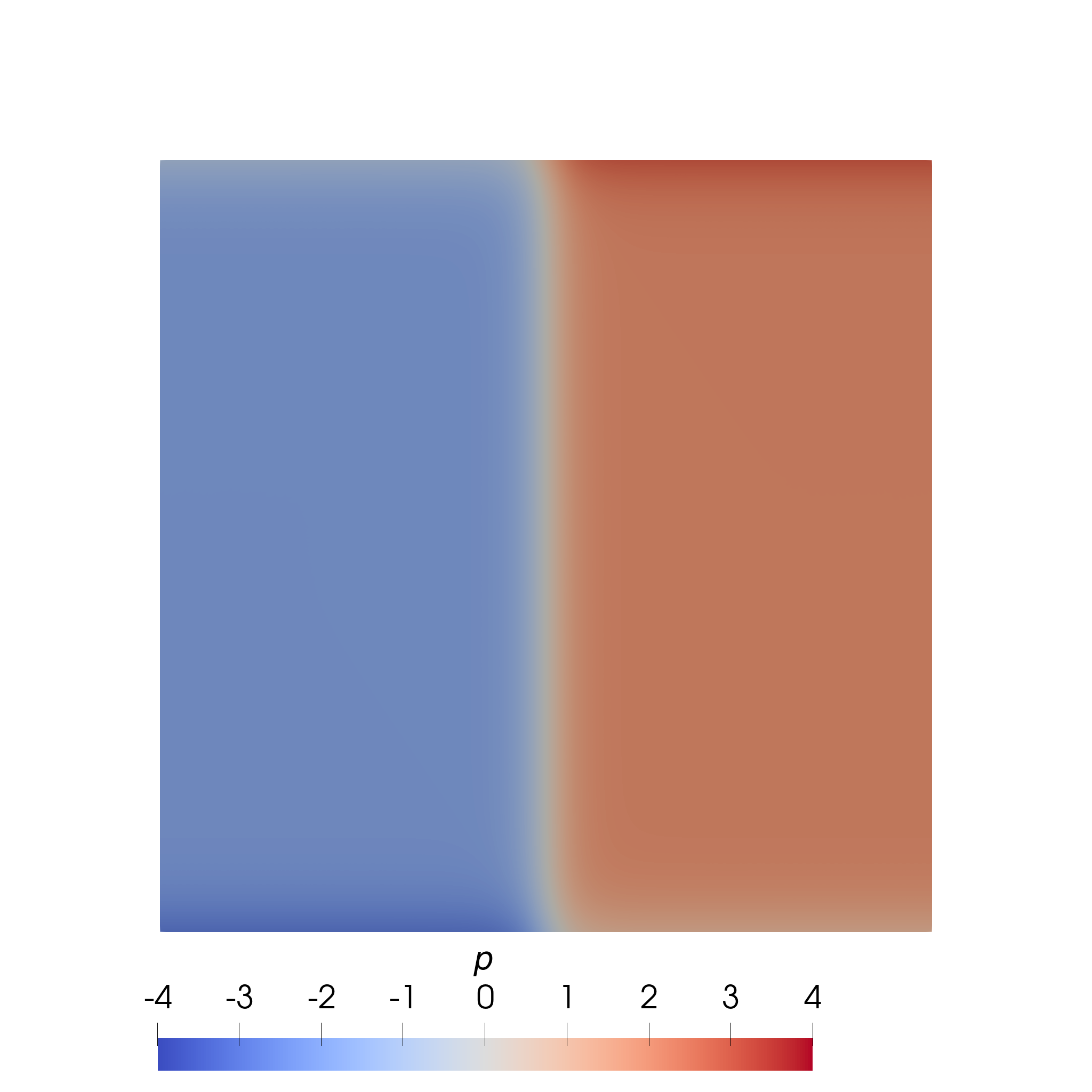
Figure 1: Pressure field $p$ for the no-flow problem at $t=0$ (left) and $t=0.725$ (right).

The impact of varying the grid, the viscosity coefficient, and the number of velocity and pressure modes on the POD-ROM errors will be studied.

For the computations we used Taylor–Hood pairs of spaces with $l=2$, i.e., continuous piecewise quadratic velocities and continuous piecewise linear pressures on the irregular triangular mesh shown in Figure 2 and its first three uniform refinements. Mesh statistics are provided in Table 1.

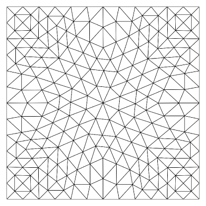
Figure 2: The computational mesh for the no-flow problem, $L=1$.

Table 1: Mesh statistics for the no-flow problem: refinement level $L$, number of triangular cells $N_{K}$, largest cell diameter $h$, velocity and pressure space dimensions.

$L$	$N_{K}$	$h$	$\mathrm{dim}(\boldsymbol{X}^{2}_{h})$	$\mathrm{dim}(Q^{1}_{h})$
1	416	0.106	1762	233
2	1664	0.053	6850	881
3	6656	0.027	27010	3425
4	26624	0.013	107266	13505

Regardless of $L$, every simulation used the BDF2 scheme as time integrator with the same relatively small time step $\Delta t=0.005$. The grid comparison in Section 5.1.1 will show that this step size was small enough to make the temporal discretization error negligible. Except in the case of the viscosity comparison presented in Section 5.1.3, the viscosity was $\nu=0.01$. We will also compare results with grad-div stabilization using $\mu=0.1$, which is a common order of magnitude for this parameter and second order Taylor–Hood elements, and without grad-div stabilization, i.e., $\mu=0$.

For each ROM computation, the reduced order velocity space $\boldsymbol{U}^{r}$ was built by applying POD with the $L^{2}(\Omega)^{d}$ inner product to the full order computation snapshots’ temporal derivatives $\tau\partial_{t}\boldsymbol{u}_{h}^{1},\ldots,\tau\partial_{t}\boldsymbol{u}_{h}^{201}$ with $\tau=1/6$ and the scaled snapshot average $\sqrt{201}\bar{\boldsymbol{u}}_{h}$. The choice of $\tau$ corresponds roughly to a characteristic time scale of $p$. The reduced order velocity was computed using (21) with $\boldsymbol{u}_{r}\in\bar{\boldsymbol{u}}_{h}+\boldsymbol{U}_{r}$. Notice that as $\boldsymbol{u}\equiv\boldsymbol{0}$, the computed velocities $\boldsymbol{u}_{h}$ and $\boldsymbol{u}_{r}$ are in all cases pure noise that should be expected to decrease with mesh refinement. It is well known that the divergence of the discrete velocity fields computed with pairs of Taylor–Hood finite elements might be quite large, e.g., see [14, Example 4.31].

Pressure modes were computed by applying POD to the pressure fluctuation snapshots $p_{h}^{1}-\bar{p}_{h},\ldots,p_{h}^{201}-\bar{p}_{h}$ to give the reduced order pressure space $\mathcal{W}^{r}$. The reduced order pressure was computed for $p_{r}\in\bar{p}_{h}+\mathcal{W}^{r}$ using both the SE-ROM method (40) and the SM-ROM method (47) with $\tau_{K}=h_{K}^{2}$.

In each case, POD modes corresponding to eigenvalues $\lambda<10^{-10}$ were discarded as noisy. Table 2 shows an overview of the results for $\nu=0.01$. The lower noise level of the velocity results with grad-div stabilization is clearly visible in the smaller number of velocity modes corresponding to large indices, as well as in the eigenvalue plots in Figure 3.

Table 2: POD statistics for the no-flow problem, $\nu=0.01$: refinement level $L$, number of velocity modes $d_{v,\mathrm{gd}}$, $d_{v,\mathrm{ngd}}$ with and without grad-div stabilization, number of pressure modes $d_{p,\mathrm{gd}}$, $d_{p,\mathrm{ngd}}$ with and without grad-div stabilization.

$L$	$d_{v,\mathrm{gd}}$	$d_{p,\mathrm{gd}}$	$d_{v,\mathrm{ngd}}$	$d_{p,\mathrm{ngd}}$
1	109	57	111	56
2	92	58	96	59
3	61	37	75	48
4	40	38	64	38

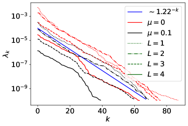
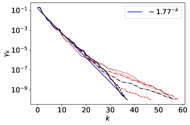
Figure 3: Velocity and pressure eigenvalues for the no-flow problem, varying grid size.

Notice that, in each comparison below, the SE-ROM and SM-ROM velocities are the same, only the pressure is computed using a different scheme.

5.1.1 Convergence with Respect to Grid Refinement

Using as many velocity and pressure modes as were available, we investigated the reduced order models’ convergence as the underlying mesh is refined.

Figure 4 shows velocity and divergence errors along with expected and empirically computed orders of convergence. These orders, three and two, respectively, meet the expectations. They are even slightly better on this range of mesh sizes. A crucial observation is that using grad-div stabilization improves both errors notably, e.g., with respect to the divergence by about an order of magnitude.

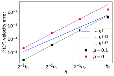
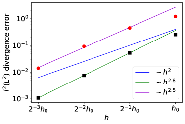
Figure 4: Velocity and divergence errors for the no-flow problem, varying grid size.

Pressure errors, along with expected and estimated orders of convergence, are presented in Figure 5. Since $X=L^{2}(\Omega)^{d}$, the error bound (4.3) is applicable, which leads to the order of convergence $h^{l-1/2}=h^{3/2}$ for the norm on the left-hand side of (4.3). Note that this norm is roughly the gradient of the pressure error multiplied by the mesh width. Again, the error reductions on the considered meshes are somewhat larger than the predicted ones. Note that the order $3/2$ is caused only from estimate (12) for the FOM pressure error and that already in the numerical studies of [9] a higher order of convergence for this error was observed. All other spatial error terms in (4.3) are of second order. The difference between the velocities with and without grad-div stabilization is too small to greatly influence the pressure errors. One can observe that the SE-ROM method gives noticeably smaller pressure errors in the $l^{2}(L^{2})$ norm compared with the SM-ROM method, but not in the $l^{2}(H^{1}_{K})$ seminorm. The $l^{2}(H^{1})$ error (not shown) also does not show a large difference.

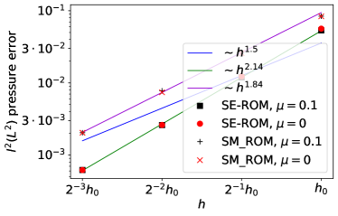
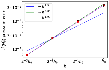
Figure 5: Pressure errors for the no-flow problem, varying grid size.

5.1.2 Convergence with Respect to Increasing Ranks

At each refinement level of the mesh, we compared the error of the reduced order models using $r\in\{2,3,4,6,8,12,16,24,32\}$ velocity and pressure modes.

For the sake of brevity and for concentrating on the topic of this paper, only results for the pressure will be presented. Notice that in each picture of Figure 6 the horizontal axis is decreasing to the right and is marked with the fraction of remaining pressure eigenvalues

$$\mathcal{R}_{p}=\sum_{k=r+1}^{d_{p}}\gamma_{k}\Bigg{/}\sum_{k=1}^{d_{p}}\gamma_{k}.$$

It becomes clear that the moving steps in $p$ do require a substantial number of pressure modes to approximate them well at all times. For decreasing $\mathcal{R}_{p}$, the graphs level off as the FOM errors eventually dominate the rank errors. There are almost no differences of the results between using the grad-div stabilization for the velocity simulations or not. Likewise, both studied methods for computing a POD-ROM pressure behave almost identically.

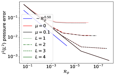
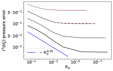
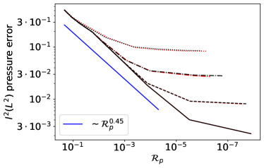
Figure 6: Pressure errors for the no-flow problem, varying number of velocity and pressure modes. Upper row: SE-ROM. Lower row: SM-ROM.

5.1.3 Impact of the Size of the Viscosity Coefficient

Finally, a study on the impact of varying the viscosity coefficient on the errors of full-rank reduced order simulations will be presented. In this study, $L=3$ was fixed and the situations that $\nu\in\{1,0.1,0.01,10^{-4},10^{-6},10^{-8}\}$ were considered.

Figure 7 shows the substantial impact of the viscosity on the presence of velocity noise (recall that $\boldsymbol{u}=\boldsymbol{0}$), particularly without grad-div stabilization. In particular, for very low viscosity coefficients the divergence error with $\mu=0.1$ is roughly three orders of magnitude smaller than with $\mu=0$ and the $l^{2}(L^{2})$ error of the velocity differs by two orders of magnitude. The errors for the simulations with grad-div stabilization are clearly robust with respect to the size of the viscosity coefficient and they are of small magnitude.

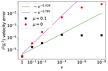
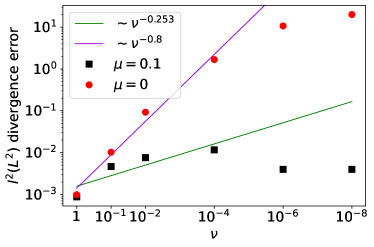
Figure 7: Velocity and divergence errors for the no-flow problem, varying viscosity.

The impact of the value of the viscosity coefficient on the POD-ROM pressure errors is shown in Figure 8. It can be seen that the errors are notably larger for small viscosity coefficients if the grad-div stabilization was not applied. For instance, for the case $\nu=10^{-8}$ we could observe that the FOM simulation without grad-div stabilization became very inaccurate towards the end of the time interval, leading to pressure snapshots with poor quality. Considering from now on only the simulations with grad-div stabilization, then the $l^{2}(L^{2})$ errors obtained with SE-ROM are a little bit smaller than the corresponding errors of the SM-ROM solutions. For $l^{2}(H_{K}^{1})$, both methods are of very similar accuracy. Clearly, the pressure errors for SE-ROM and SM-ROM are robust with respect to small values of the viscosity.

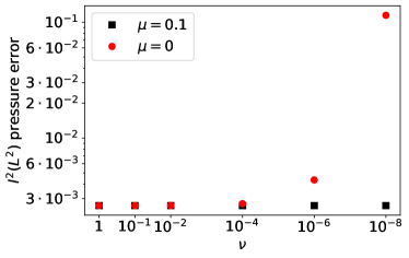
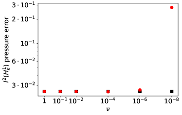
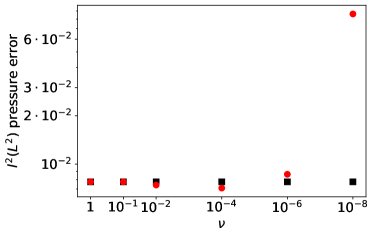
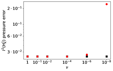
Figure 8: Pressure errors for the no-flow problem, varying viscosity. Upper row: SE-ROM. Lower row: SM-ROM.

5.1.4 Summary

The well-known benefit of grad-div stabilization on velocity errors could be seen also in this no-flow problem. It was observed, for small viscosity coefficients, that poor velocity results from FOM simulations without grad-div stabilization might have a strong impact on POD-ROM pressure errors, because the poor velocity results might induce inaccurate pressure results and thus lead to pressure snapshots of poor quality. In this respect, using grad-div stabilization is also beneficial for computing accurate POD-ROM pressure solutions. The numerical studies supported the analytic results with respect to the robustness of the errors for small viscosity coefficients and with respect to convergence orders. Concerning the error in $l^{2}(L^{2})$, using SE-ROM led to slightly more accurate results than using SM-ROM. In all other aspects, both methods behaved very similarly.

5.2 A Flow around a Cylinder

A classical example of dynamics that a reduced order model should be able to represent well is the periodic von Kármán vortex street that forms on the downstream side of an obstacle placed in the way of a constant upstream flow of moderate velocity.

We considered the classical benchmark problem defined in [23]. Let $\Omega=(0,2.2)\times(0,0.41)\setminus\bar{B}_{0.05}(0.2,0.2)$ be a rectangle with a slightly off-center disc cut out near the inlet on the left-hand side, representing a cylinder. The inlet boundary condition is prescribed by

$$\boldsymbol{u}(t;(x,y))=\left(\frac{6}{0.41^{2}}y(1-y),0\right)~{}\nicefrac{\mathrm{m}}{\mathrm{s}},\quad y\in[0,0.41].$$

At the outlet, the so-called do-nothing boundary condition is applied and on all other boundaries, a homogeneous Dirichlet condition is imposed. The kinematic viscosity of the fluid is assumed to be $\nu=0.001~{}\nicefrac{\mathrm{m^{2}}}{\mathrm{s}}$. Taking as characteristic velocity scale the mean inflow $U_{\mathrm{mean}}=1~{}\nicefrac{\mathrm{m}}{\mathrm{s}}$ and as characteristic length scale the diameter of the cylinder $\mathcal{L}=0.1~{}\mathrm{m}$, the Reynolds number of the flow is $\mathrm{Re}=100$.

Quantities of interest are the maximal drag and the maximal lift coefficients at the cylinder and the pressure difference between the front and the back of the cylinder at a certain time within the period

$$\Delta P\left(t^{*}+\frac{1}{2}T^{*}\right)=p\left(t^{*}+\frac{1}{2}T^{*};(0.15,0.2)\right)-p\left(t^{*}+\frac{1}{2}T^{*};(0.25,0.2)\right),$$

where $t^{*}$ is an appropriately defined start of the period and $T^{*}$ is the length of the period. For the exact definitions, we refer to [23] or [14, Example D.8]. In the numerical studies, the coefficients were computed by evaluating integrals on a neighborhood of the cylinder, compare [14, Example D.8]. Since this problem leads to a periodic flow field, the last quantity of interest is the Strouhal number $\mathrm{St}=\frac{\mathcal{L}}{UT^{*}}=0.1/T^{*}$, where $T^{*}$ is estimated by locating pairs of roots of $c_{\mathrm{lift}}(t)$.

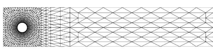
Figure 9: The computational mesh for the flow around a cylinder problem, $L=1$. Notice that this mesh is considerably finer near the cylinder than in the right-hand section of the domain.

We discretized the problem using Taylor–Hood elements with $l=2$ (continuous piecewise quadratic velocities, continuous piecewise linear pressures) on an irregular triangular mesh. The coarsest version of this mesh is shown in Figure 9. This mesh was uniformly refined, where in each refinement step the vertices on $\Gamma_{\mathrm{cyl}}$ were corrected to lie on the circle. Table 3 summarizes the mesh statistics. As temporal discretization, the BDF2 scheme with a constant time step of $\Delta t=0.005$ was utilized.

Table 3: Mesh statistics for the cylinder problem: refinement level $L$, number of triangular cells $N_{K}$, largest cell diameter $h$, velocity and pressure space dimensions.

$L$	$N_{K}$	$h$	$\mathrm{dim}(\boldsymbol{X}^{2}_{h})$	$\mathrm{dim}(Q^{1}_{h})$
1	1552	$7.17\cdot 10^{-3}$	6496	848
2	6208	$3.55\cdot 10^{-3}$	25408	3248
3	24832	$1.76\cdot 10^{-3}$	100480	12704
4	99328	$8.79\cdot 10^{-4}$	399616	50240

Results were obtained by first developing the flow from homogeneous initial conditions in the time interval $[0,8]$, by the end of which the periodic vortex shedding was well established in all simulations. Snapshots were then generated by a simulation in the interval $[8,10]$, corresponding to roughly six periods of the flow’s behavior.

As this example includes steady inhomogeneous Dirichlet boundary conditions, we did not include the average of the snapshots in the computation of the modes. Instead, we applied the POD with respect to the $L^{2}(\Omega)^{2}$ inner product to the FOM snapshots $\tau\partial_{t}\boldsymbol{u}_{h}^{1},\ldots,\tau\partial_{t}\boldsymbol{u}_{h}^{401}$, where $\tau=0.3~{}\mathrm{s}$ is roughly the length of the period, to construct a linear reduced order velocity space $\boldsymbol{U}^{r}$ and modified the velocity ROM (21) by taking $\boldsymbol{u}_{r}\in\bar{\boldsymbol{u}}_{h}+\boldsymbol{U}^{r}$, with snapshot average $\bar{\boldsymbol{u}}_{h}$, resulting in additional terms involving $\bar{\boldsymbol{u}}_{h}$ on the right-hand side of the equation in each time instant.

As before, pressure modes were computed by applying ($L^{2}(\Omega)$-)POD to the pressure fluctuation snapshots $p_{h}^{1}-\bar{p}_{h},\ldots,p_{h}^{401}-\bar{p}_{h}$ to give a reduced order pressure space $\mathcal{W}^{r}$, and both SE-ROM and SM-ROM pressures were computed for $p_{r}\in\bar{p}_{h}+\mathcal{W}^{r}$.

Table 4: POD statistics for the flow around a cylinder problem: refinement level $L$, number of velocity modes $d_{v,\mathrm{gd}}$, $d_{v,\mathrm{ngd}}$ with and without grad-div stabilization, number of pressure modes $d_{p,\mathrm{gd}}$, $d_{p,\mathrm{ngd}}$ with and without grad-div stabilization.

$L$	$d_{v,\mathrm{gd}}$	$d_{p,\mathrm{gd}}$	$d_{v,\mathrm{ngd}}$	$d_{p,\mathrm{ngd}}$
1	38	15	52	17
2	58	17	72	20
3	81	26	82	23

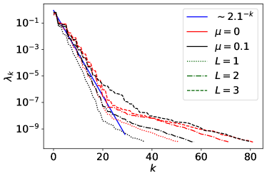
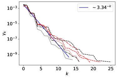
Figure 10: Velocity and pressure eigenvalues for the flow around a cylinder problem, varying grid size.

Modes corresponding to eigenvalues $\lambda<10^{-10}$ were again discarded. Table 4 shows the number of eigenvalues depending on the grid size and Figure 10 plots their decay. Note the considerably smaller number of pressure modes.

Reference intervals for the quantities of interest are defined in [23], see Table 5. For the sake of brevity, we will present only very few selected results, namely those for $L=3$, which are displayed in Table 5. As additional reference to compare with, we included statistics from a FOM computation at $L=4$ in the same time interval $[8,10]$.

Table 5: Comparison of the flow around a cylinder problem results’ to reference intervals. Here $t^{*}$ is the time in each period at which $c_{\mathrm{lift}}$ reaches its peak, and $T^{*}$ is the length of the period; this quantity is averaged over all available periods.

Model	$L$	$\mathrm{St}$	$\max(c_{\mathrm{drag}})$	$\max(c_{\mathrm{lift}})$	$\Delta P(t^{*}+\frac{1}{2}T^{*})$
Reference interval		$[0.295,0.305]$	$[3.22,3.24]$	$[0.98,1.02]$	$[2.46,2.50]$
FOM, $\mu=0$	4	0.3005	3.227	0.9839	2.484
FOM, $\mu=0$	3	0.3004	3.227	0.9848	2.485
FOM, $\mu=0.1$	3	0.3003	3.229	0.9914	2.487
SM-ROM, $\mu=0$	3	0.3014	3.221	0.9504	2.479
SM-ROM, $\mu=0.1$	3	0.3029	3.239	1.0353	2.489
SE-ROM, $\mu=0$	3	0.3003	3.229	0.8925	2.473
SE-ROM, $\mu=0.1$	3	0.3001	3.229	0.8891	2.467

The values in Table 5 were obtained with the number of POD modes given in Table 4 and they were computed by averaging the values of six subsequent periods. For the Strouhal number, the maximal drag coefficient, and the pressure difference, all values computed with the POD-ROMs, with and without grad-div stabilization and for both approaches for approximating the pressure, are within the respective reference intervals. Results of this type should be expected if all important POD modes are used and if the FOM results are already sufficiently accurate. However, the situation is different for the maximal lift coefficient, which depends strongly on the pressure approximation at the cylinder. In all POD-ROM simulations, the correct order of magnitude was obtained, but the results are outside the reference interval, with the results of SM-ROM being closer to it.

6 Summary and Outlook

This paper presents the error analysis for two ways of computing a pressure approximation in POD-ROM simulations of incompressible flow problems. Based on using a grad-div stabilization for both the FOM and the velocity POD-ROM, error bounds were derived whose constants do not blow up as the viscosity tends to zero. For the supremizer enrichment POD-ROM (SE-ROM), the presented analysis covers a different set of generating elements of the velocity ROM space than considered so far in the literature. Concerning the stabilization-motivated POD-ROM (SM-ROM), the results of the literature are improved considerably with respect to several aspects, compare the description in the Introduction. Numerical studies support the analytic results and provide an initial comparison of the behavior of both methods for computing a POD-ROM pressure.

The numerical results comparing SE-ROM and SM-ROM are not yet conclusive. Often, the results are quite similar. In the first example, the SE-ROM was more accurate with respect to the error in the $l^{2}(L^{2})$ norm and in the second example, SM-ROM was more accurate with respect to the maximal lift coefficient. Further numerical studies are needed for obtaining a better understanding of the performance of both methods in practice.

References

- [1] R. A. Adams. Sobolev spaces. Pure and Applied Mathematics, Vol. 65. Academic Press [Harcourt Brace Jovanovich, Publishers], New York-London, 1975.
- [2] D. Boffi. Stability of higher order triangular Hood-Taylor methods for the stationary Stokes equations. Math. Models Methods Appl. Sci., 4(2):223–235, 1994.
- [3] D. Boffi. Three-dimensional finite element methods for the Stokes problem. SIAM J. Numer. Anal., 34(2):664–670, 1997.
- [4] S. C. Brenner and L. R. Scott. The mathematical theory of finite element methods, volume 15 of Texts in Applied Mathematics. Springer, New York, third edition, 2008.
- [5] F. Brezzi and R. S. Falk. Stability of higher-order Hood-Taylor methods. SIAM J. Numer. Anal., 28(3):581–590, 1991.
- [6] A. Caiazzo, T. Iliescu, V. John, and S. Schyschlowa. A numerical investigation of velocity-pressure reduced order models for incompressible flows. J. Comput. Phys., 259:598–616, 2014.
- [7] T. Chacón Rebollo, S. Rubino, M. Oulghelou, and C. Allery. Error analysis of a residual-based stabilization-motivated POD-ROM for incompressible flows. Comput. Methods Appl. Mech. Engrg., 401(part B):Paper No. 115627, 2022.
- [8] P. G. Ciarlet. The finite element method for elliptic problems, volume 40 of Classics in Applied Mathematics. Society for Industrial and Applied Mathematics (SIAM), Philadelphia, PA, 2002. Reprint of the 1978 original [North-Holland, Amsterdam].
- [9] J. de Frutos, B. García-Archilla, V. John, and J. Novo. Analysis of the grad-div stabilization for the time-dependent Navier-Stokes equations with inf-sup stable finite elements. Adv. Comput. Math., 44(1):195–225, 2018.
- [10] J. de Frutos, B. García-Archilla, and J. Novo. Corrigenda: Fully discrete approximations to the time-dependent Navier-Stokes equations with a projection method in time and grad-div stabilization. J. Sci. Comput., 88(2):Paper No. 40, 3, 2021.
- [11] B. García-Archilla, V. John, and J. Novo. POD-ROMs for incompressible flows including snapshots of the temporal derivative of the full order solution. SIAM J. Numer. Anal., 2023. accepted for publication.
- [12] B. García-Archilla, J. Novo, and S. Rubino. Error analysis of proper orthogonal decomposition data assimilation schemes with grad-div stabilization for the Navier-Stokes equations. J. Comput. Appl. Math., 411:Paper No. 114246, 30, 2022.
- [13] S. Ingimarson, L. G. Rebholz, and T. Iliescu. Full and reduced order model consistency of the nonlinearity discretization in incompressible flows. Comput. Methods Appl. Mech. Engrg., 401(part B):Paper No. 115620, 16, 2022.
- [14] V. John. Finite element methods for incompressible flow problems, volume 51 of Springer Series in Computational Mathematics. Springer, Cham, 2016.
- [15] V. John, B. Moreau, and J. Novo. Error analysis of a SUPG-stabilized POD-ROM method for convection-diffusion-reaction equations. Comput. Math. Appl., 122:48–60, 2022.
- [16] K. Kean and M. Schneier. Error analysis of supremizer pressure recovery for POD based reduced-order models of the time-dependent Navier-Stokes equations. SIAM J. Numer. Anal., 58(4):2235–2264, 2020.
- [17] K. Kean and M. Schneier. Error analysis of supremizer pressure recovery for POD based reduced-order models of the time-dependent Navier-Stokes equations. SIAM J. Numer. Anal., 58(4):2235–2264, 2020.
- [18] B. Koc, S. Rubino, M. Schneier, J. Singler, and T. Iliescu. On optimal pointwise in time error bounds and difference quotients for the proper orthogonal decomposition. SIAM J. Numer. Anal., 59(4):2163–2196, 2021.
- [19] K. Kunisch and S. Volkwein. Galerkin proper orthogonal decomposition methods for parabolic problems. Numer. Math., 90(1):117–148, 2001.
- [20] S. Locke and J. Singler. New proper orthogonal decomposition approximation theory for PDE solution data. SIAM J. Numer. Anal., 58(6):3251–3285, 2020.
- [21] J. Novo and S. Rubino. Error analysis of proper orthogonal decomposition stabilized methods for incompressible flows. SIAM J. Numer. Anal., 59(1):334–369, 2021.
- [22] S. Rubino. Numerical analysis of a projection-based stabilized POD-ROM for incompressible flows. SIAM J. Numer. Anal., 58(4):2019–2058, 2020.
- [23] M. Schäfer and S. Turek. Benchmark computations of laminar flow around a cylinder. (With support by F. Durst, E. Krause and R. Rannacher). In Flow simulation with high-performance computers II. DFG priority research programme results 1993 - 1995, pages 547–566. Wiesbaden: Vieweg, 1996.
- [24] C. Taylor and P. Hood. A numerical solution of the Navier-Stokes equations using the finite element technique. Internat. J. Comput. & Fluids, 1(1):73–100, 1973.
- [25] U. Wilbrandt, C. Bartsch, N. Ahmed, N. Alia, F. Anker, L. Blank, A. Caiazzo, S. Ganesan, S. Giere, G. Matthies, R. Meesala, A. Shamim, J. Venkatesan, and V. John. ParMooN—A modernized program package based on mapped finite elements. Comput. Math. Appl., 74(1):74–88, 2017.