Promises and Pitfalls of the Linearized Laplace
in Bayesian Optimization

Abstract

The linearized-Laplace approximation (LLA) has been shown to be effective and efficient in constructing Bayesian neural networks. It is theoretically compelling since it can be seen as a Gaussian process posterior with the mean function given by the neural network’s maximum-a-posteriori predictive function and the covariance function induced by the empirical neural tangent kernel. However, while its efficacy has been studied in large-scale tasks like image classification, it has not been studied in sequential decision-making problems like Bayesian optimization where Gaussian processes—with simple mean functions and kernels such as the radial basis function—are the de-facto surrogate models. In this work, we study the usefulness of the LLA in Bayesian optimization and highlight its strong performance and flexibility. However, we also present some pitfalls that might arise and a potential problem with the LLA when the search space is unbounded.

1 Introduction

Bayesian neural networks (BNNs) have been shown to be useful for predictive uncertainty quantification, aiding tasks such as the detection of out-of-distribution data and adversarial examples (Louizos and Welling, 2016, 2017; Kristiadi et al., 2019). Recently, the Laplace approximation (LA, MacKay, 1992a) has emerged to be a compelling practical BNN method and has been successfully deployed in large-scale problems that leverage deep neural nets (NNs), such as image classification and segmentation (Barbano et al., 2022; Miani et al., 2022, etc.), due to its cost-efficiency (Daxberger et al., 2021) and its post-hoc nature. However, its performance in sequential decision-making problems in small-sample regimes—such as active learning, bandits, and Bayesian optimization—has not been studied extensively.

Nonetheless, the recently proposed linearized version of the LA (Immer et al., 2021b) has compelling benefits since it can be viewed as a Gaussian process (GP) model—the de-facto standard models used in many sequential problems like Bayesian optimization. From this perspective, the LLA is a GP with a posterior mean function given by the maximum-a-posteriori (MAP) predictive function of the NN and a covariance function given by the NN’s empirical neural tangent kernel at the MAP estimate (Jacot et al., 2018). Just like any GP, the LLA can be tuned via its differentiable marginal likelihood using standard deep learning optimizers without validation data (Immer et al., 2021a, 2022b). Unlike standard GP models, however, the LLA is much more expressive and accurate due to its NN backbone. In particular, the LLA inherits the inductive biases of the base NN and enables scalable inference due to its post-hoc formulation on top of the MAP-estimated NN.

Given its compelling theoretical benefits and its lack of usage in small-sample problems, it is thus interesting to study the performance of the LLA in this regime. In this work, we focus on Bayesian optimization and our empirical findings show that the LLA is competitive or even better than the standard GP baseline, especially when the problem requires a strong inductive bias (e.g., search in the space of images). Nevertheless, the GP view of the LLA also yields a potential pitfall in unbounded domains due to its mean function. We discuss different ideas on how the LLA can be improved in the future to mitigate this issue.

2 Linearized Laplace Approximation

Let $f:\mathcal{X}\times\Theta\to\mathcal{Y}$ be a neural network (NN) with the input, output, and parameter spaces $\mathcal{X}\subseteq\mathbb{R}^{n}$, $\mathcal{Y}\subseteq\mathbb{R}^{k}$, and $\Theta\subseteq\mathbb{R}^{d}$, respectively. Given a dataset $\mathcal{D}:=(x_{i},y_{i})_{i=1}^{m}$, the standard way to train $f$ is to find $\theta_{\text{{MAP}}}\in\Theta$ that maximizes the log-posterior function $\log p(\theta\mid\mathcal{D})$. The Laplace approximation (LA) to $p(\theta\mid\mathcal{D})$ can then be obtained by computing the Hessian $H:=-\nabla_{\theta}^{2}\log p(\theta\mid\mathcal{D})|_{\theta_{\text{{MAP}}}}$ and letting $p(\theta\mid\mathcal{D})\approx\mathcal{N}(\theta\mid\theta_{\text{{MAP}}},H^{-1})$ (MacKay, 1992b).

The generalized Gauss-Netwon (GGN) matrix is often used to approximate the exact Hessian (Martens, 2020). Since the GGN is the exact Hessian of the linearized network $f^{\mathrm{lin}}(x;\theta):=f(x;\theta_{\text{{MAP}}})+J(x)(\theta-\theta_{\text{{MAP}}})$ where $J(x):=\nabla_{\theta}f(x;\theta)\mid_{\theta_{\text{{MAP}}}}\in\mathbb{R}^{k\times d}$ is the Jacobian, it is instructive to use $f^{\mathrm{lin}}$ to make predictions under the LA, resulting in the linearized-Laplace approximation (LLA, Khan et al., 2019; Immer et al., 2021b). While the LLA depends on both the GGN and the Jacobian of the network, it is closely related to second-order optimization and thus can leverage recent advances in efficient approximations and computation in that field (Dangel et al., 2020; Osawa et al., 2023).

Due to its weight-space linearity and Gaussianity, the LLA can be seen as a Gaussian process over the function $f(x)$ directly (Immer et al., 2021b; Rasmussen and Williams, 2005). That is, it defines a prior $f\sim\mathcal{GP}(f^{\mathrm{lin}},J(x)J(x^{\prime})^{\top})$ over the function, and its posterior on a test point $x_{*}\in\mathcal{X}$ is given by the MAP prediction $f(x_{*};\theta_{\text{{MAP}}})$ with uncertainties given by the standard GP posterior variance under the (empirical, at $\theta_{\text{{MAP}}}$) neural tangent kernel (NTK, Jacot et al., 2018; Lee et al., 2018) $k(x_{1},x_{2}):=J(x_{1})J(x_{2})^{\top}$. In this view, the LLA can be seen as combining the best of both worlds: accurate predictions of a NN and calibrated uncertainties of a GP. Moreover, many methods have been proposed to improve the efficacy and efficiency of the LLA further (Kristiadi et al., 2022b, a; Antorán et al., 2023; Immer et al., 2023; Sharma et al., 2023; Bergamin et al., 2023, etc). Detailed related work is deferred to Appendix C.

3 The Linearized Laplace in Bayesian Optimization

We evaluate the LLA on three standard benchmark functions: (i) the Branin function on $[-5,10]\times[0,15]\subset\mathbb{R}^{2}$, (ii) the Ackley function on $[-32.768,32.768]^{2}\subset\mathbb{R}^{2}$, and (iii) the MNIST image generation task minimizing $f(x):=\|x-x_{0}\|$ on $[0,1]^{784}$ for a fixed $x_{0}$ taken from the MNIST training set (Verma et al., 2022). The base NNs are a three-layer ReLU MLP with $50$ hidden units each and the LeNet-5 CNN (LeCun et al., 1998), and we uniformly sample the initial training set of size $20$. Finally, the acquisition function is the popular and widely-used Expected Improvement (Jones et al., 1998). See Appendix A for the detailed experimental setup. Also, refer to Aerni (2022) for a comparison of the LLA on sequential decision-making problems, and to the parallel work by Li et al. (2023) for a comprehensive benchmark of BNN-based (including the LLA) Bayesian optimization surrogates against GPs. The BoTorch implementation of the LLA surrogate is available at https://github.com/wiseodd/laplace-bayesopt.

3.1 Experiment results

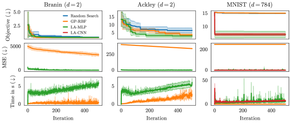
Figure 1: Bayesian optimization experiments in terms of objective minimization (top), predictive accuracies of the surrogate models (middle), and the wall-clock time (in seconds) taken to propose a new evaluation point (bottom). The LLA methods outperform the GP on the more complex problems.

The results are shown in Fig. 1. In terms of optimization performance, the LLA is competitive or even better than the (tuned) GP baseline on all benchmark functions. On the high-dimensional MNIST problem, GP-RBF performs similarly (bad) as the random search baseline. Meanwhile, the LLA finds an $x$ with small $f(x)$ in a few iterations. While the MLP- and CNN-based LLA perform similarly in terms of the mean, the CNN-based LLA is considerably less noisy. This indicates that LLA-CNN is more reliable that LLA-MLP in finding the minimizers of the objective function. All in all, the better performance of the LLA can be contributed to the strong predictive performance (in terms of test mean-squared error) of the base NNs.

In terms of computation cost, the LLA induces some overhead compared to the (exact) GP-RBF. This is because, at each iteration, the acquisition function needs to be optimized by backpropagating through the NN and its Jacobian. Nevertheless, we found that the LLA is more memory-efficient than the exact GP due to the fact that it can leverage mini-batching. Meanwhile, the GP can quickly yield an out-of-memory error (after around $800$ iterations). While both GPs and the LLA can leverage sparse posterior approximations (Titsias, 2009), unlike standard GPs, the LLA has the advantage that it is both parametric and non-parametric (Section 2) and thus one can pick a cheaper inference procedure (i.e., in weight space or function space) depending the amount of data at hand and the size of the network (Immer et al., 2023).

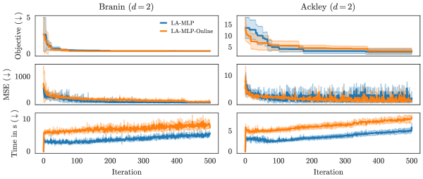
Figure 2: Post-hoc vs. online LLA in Bayesian optimization, in terms of objective minimization (top), predictive accuracies of the surrogate models (middle), and the wall-clock time (in seconds) taken to propose a new evaluation point (bottom). The post-hoc LLA tends to perform at least on par with the online one while being computationally cheaper.

Finally, we compare the two popular methods for tuning LLA: online (Immer et al., 2021a) and post hoc (Kristiadi et al., 2020, 2021a; Eschenhagen et al., 2021). We found that post-hoc LLA performs similarly to the online LLA while being cheaper since the marginal likelihood tuning is only being done once after the MAP training (see Fig. 2). This is encouraging because the strong performance of the LLA thus can be obtained at a low cost. Note that, this finding agrees with the conclusion of Aerni (2022).

In Appendix B, we further show empirical evidence regarding the capabilities of the LLA in small-sample regimes. These results further reaffirm the effectiveness of the LLA in Bayesian optimization, and possibly in other sequential problems.

3.2 Pitfalls

We have seen empirically that the LLA can be useful in sequential problems with bounded domains. However, the function-space interpretation of the LLA posterior—MAP-estimated NN as its mean function and the corresponding empirical (i.e. finite-width) NTK kernel as its covariance function—can be a double-edged sword in general. Specifically, Hein et al. (2019) have shown that ReLU networks, the most popular NN architecture, perform pathologically in the extrapolation regime outside of the data in the sense that $f(\,\cdot\,;\theta_{\text{{MAP}}})$ is a non-constant linear function, i.e., always increasing or decreasing. Thus, when a ReLU NN is used in the LLA, the LLA will inherit this behavior. As a surrogate function, this ReLU LLA will then behave pathologically under commonly-used acquisition functions $\alpha$: The acquisition function will always pick $x\in\mathcal{X}$ that maximizes $\alpha$ under $f(x;\theta_{\text{{MAP}}})$ and its uncertainty—but when $f(x;\theta_{\text{{MAP}}})$ is always increasing (or decreasing) outside the data, $\alpha$ will always yield points that are far away from the current data (see Fig. 3).

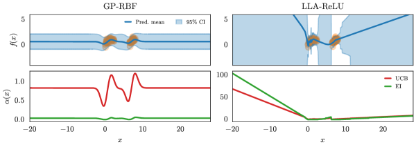
Figure 3: As a surrogate function, LLA with ReLU activations is (pathologically) always increasing/decreasing far away from the data. This impacts popular acquisition functions like UCB and EI and thus the exploration-exploitation behavior.

While Kristiadi et al. (2020, 2021b) have shown that the LLA’s uncertainty can be sufficient in counterbalancing the linear growth of the mean function in classification, this mitigation is absent in regression—the standard problem formulation in Bayesian optimization. For instance, let

$$\alpha(x):=f(x;\theta_{\text{{MAP}}})+\beta\sigma(x)$$ (1)

with $\beta>0$ be the UCB (Garivier and Moulines, 2011) under the LLA posterior, where $\sigma^{2}(x)$ is the GP posterior variance on $x$ under the empirical NTK kernel. Then, since outside of the data region, $f(x;\theta_{\text{{MAP}}})$ and $\sigma(x)$ is always increasing/decreasing linearly in $x$ (Kristiadi et al., 2020), it is easy to see that $\alpha(x)$ is also increasing/decreasing linearly in $x$. Since the goal is to obtain a next point $x_{t+1}=\operatorname*{arg\,max}_{x}\alpha(x)$ that maximizes/minimizes $\alpha$, the proposed $x_{t+1}$ will always be far away from the current data (infinitely so when $\mathcal{X}$ is an unbounded space).

While solving this issue is beyond the scope of the present work, one can follow the following recommendation to mitigate the aforementioned pathology, to some degree (Fig. 4): (i) specify the upper and lower bounds on the possible values of $x$, and (ii) use random points, sampled uniformly from inside the bounds, to initialize the training data for the LLA.

Beyond the above “hotfix”, possible solutions are (i) better architectural design, e.g., using more suitable activation functions (Meronen et al., 2021), and (ii) designing an acquisition function that takes the behavior induced by the MAP-estimated network into account. For instance, one option for the latter could be to avoid the asymptotic regions of the ReLU network altogether. While this restricts the exploration to be regions near the already gathered data, similar to proximal or trust-region methods (Schulman et al., 2015, 2017), it might be worth paying this price to harness the capabilities of neural networks, like strong inductive bias and good predictive accuracy.

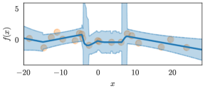
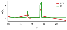
Figure 4: By (i) specifiying bounds on $x$, (ii) initialize the training data uniformly at random, one can mitigate the pathology to some degree.

4 Conclusion

We have empirically validated the effectiveness of the linearized Laplace in Bayesian optimization problems: It can outperform standard Gaussian process baselines, especially in tasks where strong inductive biases are beneficial, e.g., when the search space consists of images. The linearized Laplace provides flexibility to the practitioners in incorporating the inductive bias due to its Gaussian-process interpretation: its posterior mean is given by the neural network’s MAP predictive function and its posterior mean is induced by the empirical neural tangent kernel of the network. The former implies that the predictive mean of the linearized Laplace directly encodes the inductive bias of the base NN.

On the other hand, the aforementioned properties of the linearized Laplace yield a pitfall in Bayesian optimization. Namely, the MAP predictive functions of ReLU networks are known to be pathological: they are always increasing or decreasing outside of the data. Moreover, the induced neural tangent kernel is non-stationary, unlike the commonly-used kernel in Bayesian optimization. They can thus yield pathological behavior in unbounded domains when used in conjunction with standard acquisition functions. The investigation of this issue is an interesting direction for future work.

Resources used in preparing this research were provided, in part, by the Province of Ontario, the Government of Canada through CIFAR, and companies sponsoring the Vector Institute. VF was supported by a Branco Weiss Fellowship.

Appendix A Experiment Details

In the following, we describe the experimental setup we used to obtain the Bayesian optimization results presented in the main text.

Models

For the MLP model, the architecture is $n-50-50-1$. Meanwhile, for the CNN model, the architecture is the LeNet-5 (LeCun et al., 1998) where the two last dense hidden layers are of size $50$ and $20$.

Training

For all methods (including the baselines), we initialize the starting dataset by uniformly sampling the search space and obtain the target by evaluating the true objective values on those samples. For both models, we train them for $1000$ epochs with full batch ADAM and cosine-annealed learning rate scheduler. The starting learning rate and weight decay pairs are ($1\text{\times}{10}^{-1}$, $1\text{\times}{10}^{-3}$) and ($1\text{\times}{10}^{-3}$, $5\text{\times}{10}^{-4}$) for the MLP and CNN models, respectively. For the LLA, the marginal likelihood optimization is done for $10$ iterations. For the online LLA, this optimization is done every $50$ epochs of the “outer” ADAM optimization loop. For the other hyperparameters for the marginal likelihood optimization, we follow Immer et al. (2021a).

Baselines

The random search baseline is done by uniformly sampling from the search domain. Meanwhile, for the GP-RBF baseline, we use the standard setup provided by BoTorch (Balandat et al., 2020). In particular, it is tuned by maximizing its marginal likelihood.

Appendix B Additional Experiments

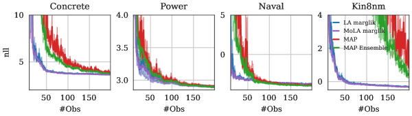
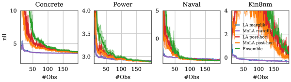
Figure 5: Test negative log-likelihood (nll) for UCI regression datasets with MAP prediction (not Bayesian) of MAP optimized models and model trained with marginal likelihood optimization (“marglik”) during training as in (Immer et al., 2021a). All methods were trained on $1-200$ observation points, where in each turn, one observation point is added. “MoLA” indicates a mixture of Laplace approximations with the same number of components as the deep ensemble. The online marginal-likelihood optimization methods outperform simple MAP with fixed prior precision.

Figure 6: Test negative log-likelihood (nll) on the same four UCI regression data sets but instead with the Bayesian posterior predictive of the Laplace approximation (i.e. via Bayesian model averaging) in comparison to the same deep ensemble as in the figure above. The online marginal-likelihood optimization methods again clearly outperform the others. “post-hoc” is a Laplace approximation trained with a fixed prior precision and optimizes it after training. Interestingly, the Bayesian predictive helps the unimodal MAP to improve over the deep ensemble and MoLA does so even more. Overall, using the Bayesian predictive tends to improve the performance for all models.

B.1 Small-Data Regression

Results

In Fig. 6 and Fig. 6, we compare the Laplace approximation methods to a deep ensemble of five neural networks on four UCI regression datasets. The models are trained on small increasing subsets from one to $200$ data points and evaluated on a held-out validation set consisting of the held-out data points. The mixture of Laplace (MoLA) variants are trained with the same number of components as the deep ensemble. We show results for post-hoc Laplace approximation, which is trained with a fixed prior precision and optimizes it after training (MacKay, 1992a; Eschenhagen et al., 2021), and marglik Laplace approximation, which is trained with Laplace marginal likelihood optimization during training (Immer et al., 2021a).

The results show that the online marginal likelihood optimization performs best early during training with the mixture and single Laplace performing similarly well. Further, the methods clearly improve when using the Bayesian posterior predictive in Fig. 6 compared to the MAP prediction in Fig. 6. This is clearly visible by comparing post-hoc MoLA to the Ensemble method (Lakshminarayanan et al., 2017), which is the same model but predicts with the MAP of the individual models instead of their Laplace approximation (Eschenhagen et al., 2021). Even post-hoc Laplace can outperform the Ensemble, despite only using a single model.

Setup

All models are MLPs with fifty hidden units and ReLU activation. We train the methods on one to $200$ training points, in each turn adding a single data point, and repeat this for three runs. The test (predictive) log-likelihood is reported over three runs with standard error. All models are trained for $1000$ steps using Adam (Kingma and Ba, 2015) with a learning rate of $1\text{\times}{10}^{-3}$ decayed to $1\text{\times}{10}^{-5}$. The online marginal likelihood variant optimizes every $50$ steps for $50$ hyperparameter steps and uses early stopping on the marginal likelihood value (Immer et al., 2021a). The post-hoc variant optimizes the hyperparameters after training for $1000$ steps and uses the last-layer posterior predictive instead of the full-network predictive since it becomes less stable when applied after training without optimizing the prior precision with either cross-validation or the marginal likelihood during training.

Method	Normalized KL $\downarrow$	Test Accuracy $\uparrow$
Uniform	1.000 $\pm$ 0.007	0.4735
MLP	0.391 $\pm$ 0.171	0.9159
Ensemble	0.381 $\pm$ 0.163	0.9161
LA post-hoc	0.643 $\pm$ 0.064	0.9147
LA marglik	0.567 $\pm$ 0.064	0.9157

Table 1: Results on the CLASSIFICATION_2D_TEST sweep of the Neural Testbed. Surprisingly, both Laplace approximation variations are worse than the simple baselines in terms of the KL-metric proposed by (Wen et al., 2021).

B.2 Evaluating Joint Predictions on the Neural Testbed

Traditionally, the Bayesian deep learning literature focuses on marginal predictions on individual data points (c.f. Appendix C). However, Wen et al. (2021) argue that joint predictive distributions, i.e. predicting a set of labels from a set of inputs, which can capture correlations between predictions on different data points, is much more important for downstream task performance, e.g. in sequential decision making. To facilitate the evaluation of the joint predictive distribution of agents, Osband et al. (2022) propose a simple benchmark of randomly generated classification problems, called the Neural Testbed. While it only consists of small-scale and artificial tasks, the goal is to have a “sanity check” for uncertainty quantification methods in deep learning, to judge their potential on more realistic problems and help guide future research. The authors also show empirically that the performance of the joint predictive is correlated with regret in bandit problems (Gittins, 1979), whereas the marginal predictive performance is not.

Recall that the linearized Laplace is a GP: It naturally gives rise to a joint predictive distribution over input points. However, Laplace approximation-based methods have not been evaluated on this benchmark yet. Here, we include preliminary results on the CLASSIFICATION_2D_TEST subset of the benchmark.

Setup

As in the experiments in Section B.1, all models are MLPs with fifty hidden units and ReLU activations. We optimize for $100$ epochs using Adam with a learning rate of $1\text{\times}{10}^{-3}$. We train on CLASSIFICATION_2D_TEST, a set of seven $2$D binary classification problems. Each method is evaluated on a test set by calculating an approximation to the expected Kullback-Leibler (KL) divergence between the predictive distribution under the method and the true ground-truth data generating process. We normalize the KL divergence to $1.0$ for our reference agent which predicts uniform class probabilities. See Osband et al. (2022) for more details.

For the post-hoc tuning of the prior precision we optimize the marginal likelihood once after training and use a last-layer Laplace approximation with full covariance. For the online tuning of the prior precision via optimizing the Laplace marginal likelihood, we use a burn-in of $20$ steps and then take $50$ optimization steps every five training steps. Here, we use a Laplace approximation over all weights with a Kronecker factored covariance and a layer-wise prior precision. For both variations of the method, we approximate the predictive using the probit approximation (Spiegelhalter and Lauritzen, 1990; MacKay, 1992b). In addition, we tried different predictive approximations, but got comparable results.

Results

In Table 1, we can see results for a regular MLP, a deep ensemble, and the Laplace approximation. Surprisingly, both variations of the LA perform significantly worse in terms of KL divergence compared to the MLP and the deep ensemble, while the test accuracy is comparable. Online marginal likelihood optimization performs better than post-hoc, but since both are so much worse than the simple baselines, the significance of this difference is unclear. Since we would expect the Laplace approximation to do at least as well as the MLP, we think further investigating the discrepancy in performance is a important step towards applying the Laplace approximation to sequential decision making problems. Also, the results demonstrate the potential pitfalls of expecting Bayesian deep learning techniques to work out-of-the-box in new settings.

Appendix C Related Work

Bayesian neural networks

Bayesian neural networks promise to combine the expressivity of neural networks with the principled statistical properties of Bayesian inference (MacKay, 1992c; Neal, 1993). However, since their inception, performing approximate inference in these complex models has remained a lingering challenge (Jospin et al., 2022). Since exact inference is intractable, approximate inference techniques follow a natural tradeoff between quality and computational cost, from cheap local approximations like Laplace inference (Laplace, 1774; MacKay, 1992c; Khan et al., 2019; Daxberger et al., 2021), stochastic weight averaging (Izmailov et al., 2018; Maddox et al., 2019), and dropout (Gal and Ghahramani, 2016; Kingma et al., 2015), via variational approximations with different levels of complexity (e.g., Graves, 2011; Blundell et al., 2015; Louizos and Welling, 2016; Khan et al., 2018; Osawa et al., 2019), across ensemble-based methods (Lakshminarayanan et al., 2017; Wang et al., 2019; Wilson and Izmailov, 2020; Ciosek et al., 2020; He et al., 2020; D’Angelo et al., 2021; D’Angelo and Fortuin, 2021; Eschenhagen et al., 2021), up to the very expensive but asymptotically correct Markov Chain Monte Carlo (MCMC) approaches (e.g., Neal, 1993; Neal et al., 2011; Welling and Teh, 2011; Garriga-Alonso and Fortuin, 2021; Izmailov et al., 2021). Apart from the challenges relating to approximate inference, recent work has also studied the question of how to choose appropriate priors for BNNs (e.g., Fortuin et al., 2021, 2022; Nabarro et al., 2022; Sharma et al., 2023; Fortuin, 2022, and references therein) and how to effectively perform model selection in this framework (e.g., Immer et al., 2021a, 2022a, 2022b; Rothfuss et al., 2021, 2022; van der Ouderaa and van der Wilk, 2022; Schwöbel et al., 2022). In our work, we particularly draw on the recent advances in Laplace inference (Daxberger et al., 2021), particularly linearized Laplace (MacKay, 1992b; Immer et al., 2021b), and its associated marginal-likelihood-based model selection capabilities (Immer et al., 2021a). However, we apply these methods to the sequential learning setting, especially Bayesian optimization, which to the best of our knowledge has not been studied before.

Bayesian optimization

While Bayesian optimization (BO) has been intensely studied (Shahriari et al., 2015; Garnett, 2023, and references therein), the de-facto standard models for this purpose have been Gaussian processes (GPs) (Rasmussen and Williams, 2005; Balandat et al., 2020; Gardner et al., 2018). Indeed, existing work using BNNs as surrogate models for BO is scarce (Snoek et al., 2015; Springenberg et al., 2016; Kim et al., 2021; Rothfuss et al., 2021) and all these approaches use either Bayesian linear regression (Snoek et al., 2015), MCMC (Springenberg et al., 2016), or ensemble-based inference (Kim et al., 2021; Rothfuss et al., 2021). To the best of our knowledge, we are the first to propose Laplace inference for this problem and highlight its performance benefits, low computational cost, and model selection capabilities.

References

- Aerni (2022) Michael Aerni. On the Laplace approximation for sequential model selection of Bayesian neural networks. Master’s thesis, ETH Zurich, 2022.
- Antorán et al. (2023) Javier Antorán, Shreyas Padhy, Riccardo Barbano, Eric Nalisnick, David Janz, and José Miguel Hernández-Lobato. Sampling-based inference for large linear models, with application to linearised Laplace. In ICLR, 2023.
- Balandat et al. (2020) Maximilian Balandat, Brian Karrer, Daniel R. Jiang, Sam Daulton, Benjamin Letham, Andrew Gordon Wilson, and Eytan Bakshy. BoTorch: A framework for efficient Monte-Carlo Bayesian optimization. In NeurIPS, 2020.
- Barbano et al. (2022) Riccardo Barbano, Johannes Leuschner, Javier Antorán, Bangti Jin, and José Miguel Hernández-Lobato. Bayesian experimental design for computed tomography with the linearised deep image prior. In ICML Workshop on Adaptive Experimental Design and Active Learning, 2022.
- Bergamin et al. (2023) Federico Bergamin, Pablo Moreno-Muñoz, Søren Hauberg, and Georgios Arvanitidis. Riemannian Laplace approximations for Bayesian neural networks. arXiv preprint arXiv:2306.07158, 2023.
- Blundell et al. (2015) Charles Blundell, Julien Cornebise, Koray Kavukcuoglu, and Daan Wierstra. Weight uncertainty in neural networks. In ICML, 2015.
- Ciosek et al. (2020) Kamil Ciosek, Vincent Fortuin, Ryota Tomioka, Katja Hofmann, and Richard Turner. Conservative uncertainty estimation by fitting prior networks. In ICLR, 2020.
- Dangel et al. (2020) Felix Dangel, Frederik Kunstner, and Philipp Hennig. BackPACK: Packing more into backprop. In ICLR, 2020.
- D’Angelo and Fortuin (2021) Francesco D’Angelo and Vincent Fortuin. Repulsive deep ensembles are Bayesian. In NeurIPS, 2021.
- D’Angelo et al. (2021) Francesco D’Angelo, Vincent Fortuin, and Florian Wenzel. On Stein variational neural network ensembles. arXiv preprint arXiv:2106.10760, 2021.
- Daxberger et al. (2021) Erik Daxberger, Agustinus Kristiadi, Alexander Immer, Runa Eschenhagen, Matthias Bauer, and Philipp Hennig. Laplace redux–effortless Bayesian deep learning. In NeurIPS, 2021.
- Eschenhagen et al. (2021) Runa Eschenhagen, Erik Daxberger, Philipp Hennig, and Agustinus Kristiadi. Mixtures of Laplace approximations for improved post-hoc uncertainty in deep learning. In NeurIPS Workshop of Bayesian Deep Learning, 2021.
- Fortuin (2022) Vincent Fortuin. Priors in Bayesian deep learning: A review. International Statistical Review, 90(3), 2022.
- Fortuin et al. (2021) Vincent Fortuin, Adrià Garriga-Alonso, Mark van der Wilk, and Laurence Aitchison. BNNpriors: A library for Bayesian neural network inference with different prior distributions. Software Impacts, 9, 2021.
- Fortuin et al. (2022) Vincent Fortuin, Adrià Garriga-Alonso, Sebastian W Ober, Florian Wenzel, Gunnar Ratsch, Richard E Turner, Mark van der Wilk, and Laurence Aitchison. Bayesian neural network priors revisited. In ICLR, 2022.
- Gal and Ghahramani (2016) Yarin Gal and Zoubin Ghahramani. Dropout as a Bayesian approximation: Representing model uncertainty in deep learning. In ICML, 2016.
- Gardner et al. (2018) Jacob Gardner, Geoff Pleiss, Kilian Q Weinberger, David Bindel, and Andrew G Wilson. GPyTorch: Blackbox matrix-matrix Gaussian process inference with GPU acceleration. In NIPS, 2018.
- Garivier and Moulines (2011) Aurélien Garivier and Eric Moulines. On upper-confidence bound policies for switching bandit problems. In ALT, 2011.
- Garnett (2023) Roman Garnett. Bayesian optimization. Cambridge University Press, 2023.
- Garriga-Alonso and Fortuin (2021) Adrià Garriga-Alonso and Vincent Fortuin. Exact Langevin dynamics with stochastic gradients. arXiv preprint arXiv:2102.01691, 2021.
- Gittins (1979) John C. Gittins. Bandit processes and dynamic allocation indices. Journal of the royal statistical society series b-methodological, 41:148–164, 1979.
- Graves (2011) Alex Graves. Practical variational inference for neural networks. In NIPS, 2011.
- He et al. (2020) Bobby He, Balaji Lakshminarayanan, and Yee Whye Teh. Bayesian deep ensembles via the neural tangent kernel. In NeurIPS, 2020.
- Hein et al. (2019) Matthias Hein, Maksym Andriushchenko, and Julian Bitterwolf. Why ReLU networks yield high-confidence predictions far away from the training data and how to mitigate the problem. In CVPR, 2019.
- Immer et al. (2021a) Alexander Immer, Matthias Bauer, Vincent Fortuin, Gunnar Rätsch, and Mohammad Emtiyaz Khan. Scalable marginal likelihood estimation for model selection in deep learning. In ICML, 2021a.
- Immer et al. (2021b) Alexander Immer, Maciej Korzepa, and Matthias Bauer. Improving predictions of Bayesian neural nets via local linearization. In AISTATS, 2021b.
- Immer et al. (2022a) Alexander Immer, Lucas Torroba Hennigen, Vincent Fortuin, and Ryan Cotterell. Probing as quantifying inductive bias. In ACL, 2022a.
- Immer et al. (2022b) Alexander Immer, Tycho FA van der Ouderaa, Vincent Fortuin, Gunnar Rätsch, and Mark van der Wilk. Invariance learning in deep neural networks with differentiable Laplace approximations. In NeurIPS, 2022b.
- Immer et al. (2023) Alexander Immer, Tycho FA van der Ouderaa, Mark van der Wilk, Gunnar Rätsch, and Bernhard Schölkopf. Stochastic marginal likelihood gradients using neural tangent kernels. In ICML, 2023.
- Izmailov et al. (2018) Pavel Izmailov, Dmitrii Podoprikhin, Timur Garipov, Dmitry Vetrov, and Andrew Gordon Wilson. Averaging weights leads to wider optima and better generalization. In UAI, 2018.
- Izmailov et al. (2021) Pavel Izmailov, Sharad Vikram, Matthew D Hoffman, and Andrew Gordon Wilson. What are Bayesian neural network posteriors really like? In ICML, 2021.
- Jacot et al. (2018) Arthur Jacot, Franck Gabriel, and Clément Hongler. Neural tangent kernel: Convergence and generalization in neural networks. In NIPS, 2018.
- Jones et al. (1998) Donald R Jones, Matthias Schonlau, and William J Welch. Efficient global optimization of expensive black-box functions. Journal of Global optimization, 13(4), 1998.
- Jospin et al. (2022) Laurent Valentin Jospin, Hamid Laga, Farid Boussaid, Wray Buntine, and Mohammed Bennamoun. Hands-on Bayesian neural networks - a tutorial for deep learning users. IEEE Computational Intelligence Magazine, 17(2), 2022.
- Khan et al. (2018) Mohammad Khan, Didrik Nielsen, Voot Tangkaratt, Wu Lin, Yarin Gal, and Akash Srivastava. Fast and scalable Bayesian deep learning by weight-perturbation in Adam. In ICML, 2018.
- Khan et al. (2019) Mohammad Emtiyaz E Khan, Alexander Immer, Ehsan Abedi, and Maciej Korzepa. Approximate inference turns deep networks into Gaussian processes. In NeurIPS, 2019.
- Kim et al. (2021) Samuel Kim, Peter Y Lu, Charlotte Loh, Jamie Smith, Jasper Snoek, and Marin Soljačić. Scalable and flexible deep Bayesian optimization with auxiliary information for scientific problems. TMLR, 2021.
- Kingma and Ba (2015) Diederik P Kingma and Jimmy Ba. Adam: A method for stochastic optimization. In ICLR, 2015.
- Kingma et al. (2015) Diederik P Kingma, Tim Salimans, and Max Welling. Variational dropout and the local reparameterization trick. In Advances in Neural Information Processing Systems 28. 2015.
- Kristiadi et al. (2019) Agustinus Kristiadi, Sina Däubener, and Asja Fischer. Predictive uncertainty quantification with compound density networks. In NeurIPS Workshop in Bayesian Deep Learning, 2019.
- Kristiadi et al. (2020) Agustinus Kristiadi, Matthias Hein, and Philipp Hennig. Being Bayesian, even just a bit, fixes overconfidence in ReLU networks. In ICML, 2020.
- Kristiadi et al. (2021a) Agustinus Kristiadi, Matthias Hein, and Philipp Hennig. Learnable uncertainty under Laplace approximations. In UAI, 2021a.
- Kristiadi et al. (2021b) Agustinus Kristiadi, Matthias Hein, and Philipp Hennig. An infinite-feature extension for Bayesian ReLU nets that fixes their asymptotic overconfidence. In NeurIPS, 2021b.
- Kristiadi et al. (2022a) Agustinus Kristiadi, Runa Eschenhagen, and Philipp Hennig. Posterior refinement improves sample efficiency in Bayesian neural networks. In NeurIPS, 2022a.
- Kristiadi et al. (2022b) Agustinus Kristiadi, Matthias Hein, and Philipp Hennig. Being a bit frequentist improves Bayesian neural networks. In AISTATS, 2022b.
- Lakshminarayanan et al. (2017) Balaji Lakshminarayanan, Alexander Pritzel, and Charles Blundell. Simple and scalable predictive uncertainty estimation using deep ensembles. In NIPS, 2017.
- Laplace (1774) Pierre-Simon Laplace. Mémoires de mathématique et de physique, tome sixieme. 1774.
- LeCun et al. (1998) Yann LeCun, Léon Bottou, Yoshua Bengio, and Patrick Haffner. Gradient-based learning applied to document recognition. Proceedings of the IEEE, 86(11), 1998.
- Lee et al. (2018) Jaehoon Lee, Yasaman Bahri, Roman Novak, Samuel S Schoenholz, Jeffrey Pennington, and Jascha Sohl-Dickstein. Deep neural networks as Gaussian processes. In ICLR, 2018.
- Li et al. (2023) Yucen Lily Li, Tim GJ Rudner, and Andrew Gordon Wilson. A study of Bayesian neural network surrogates for Bayesian optimization. arXiv preprint arXiv:2305.20028, 2023.
- Louizos and Welling (2016) Christos Louizos and Max Welling. Structured and efficient variational deep learning with matrix Gaussian posteriors. In ICML, 2016.
- Louizos and Welling (2017) Christos Louizos and Max Welling. Multiplicative normalizing flows for variational Bayesian neural networks. In ICML, 2017.
- MacKay (1992a) David JC MacKay. Bayesian interpolation. Neural computation, 4(3), 1992a.
- MacKay (1992b) David JC MacKay. The evidence framework applied to classification networks. Neural Computation, 4(5), 1992b.
- MacKay (1992c) David JC MacKay. A practical Bayesian framework for backpropagation networks. Neural Computation, 4(3), 1992c.
- Maddox et al. (2019) Wesley J Maddox, Pavel Izmailov, Timur Garipov, Dmitry P Vetrov, and Andrew Gordon Wilson. A simple baseline for Bayesian uncertainty in deep learning. In NeurIPS, 2019.
- Martens (2020) James Martens. New insights and perspectives on the natural gradient method. JMLR, 21(146), 2020.
- Meronen et al. (2021) Lassi Meronen, Martin Trapp, and Arno Solin. Periodic activation functions induce stationarity. In NeurIPS, 2021.
- Miani et al. (2022) Marco Miani, Frederik Warburg, Pablo Moreno-Muñoz, Nicki Skafte, and Søren Hauberg. Laplacian autoencoders for learning stochastic representations. In NeurIPS, 2022.
- Nabarro et al. (2022) Seth Nabarro, Stoil Ganev, Adrià Garriga-Alonso, Vincent Fortuin, Mark van der Wilk, and Laurence Aitchison. Data augmentation in Bayesian neural networks and the cold posterior effect. In UAI, 2022.
- Neal (1993) Radford M Neal. Bayesian learning via stochastic dynamics. In NIPS, 1993.
- Neal et al. (2011) Radford M Neal et al. MCMC using Hamiltonian dynamics. Handbook of Markov Chain Monte Carlo, 2(11), 2011.
- Osawa et al. (2019) Kazuki Osawa, Siddharth Swaroop, Mohammad Emtiyaz E Khan, Anirudh Jain, Runa Eschenhagen, Richard E Turner, and Rio Yokota. Practical deep learning with Bayesian principles. In NeurIPS, 2019.
- Osawa et al. (2023) Kazuki Osawa, Satoki Ishikawa, Rio Yokota, Shigang Li, and Torsten Hoefler. ASDL: A unified interface for gradient preconditioning in PyTorch. arXiv preprint arXiv:2305.04684, 2023.
- Osband et al. (2022) Ian Osband, Zheng Wen, Seyed Mohammad Asghari, Vikranth Reddy Dwaracherla, Botao Hao, Morteza Ibrahimi, Dieterich Lawson, Xiuyuan Lu, Brendan O’Donoghue, and Benjamin Van Roy. The neural testbed: Evaluating predictive distributions. In NeurIPS, 2022.
- Rasmussen and Williams (2005) Carl Edward Rasmussen and Christopher K. I. Williams. Gaussian processes in machine learning. 2005.
- Rothfuss et al. (2021) Jonas Rothfuss, Vincent Fortuin, Martin Josifoski, and Andreas Krause. Pacoh: Bayes-optimal meta-learning with pac-guarantees. In ICML, 2021.
- Rothfuss et al. (2022) Jonas Rothfuss, Martin Josifoski, Vincent Fortuin, and Andreas Krause. PAC-Bayesian meta-learning: From theory to practice. arXiv preprint arXiv:2211.07206, 2022.
- Schulman et al. (2015) John Schulman, Sergey Levine, Pieter Abbeel, Michael Jordan, and Philipp Moritz. Trust region policy optimization. In ICML, 2015.
- Schulman et al. (2017) John Schulman, Filip Wolski, Prafulla Dhariwal, Alec Radford, and Oleg Klimov. Proximal policy optimization algorithms. arXiv preprint arXiv:1707.06347, 2017.
- Schwöbel et al. (2022) Pola Schwöbel, Martin Jørgensen, Sebastian W Ober, and Mark Van Der Wilk. Last layer marginal likelihood for invariance learning. In AISTATS, 2022.
- Shahriari et al. (2015) Bobak Shahriari, Kevin Swersky, Ziyu Wang, Ryan P Adams, and Nando De Freitas. Taking the human out of the loop: A review of Bayesian optimization. Proceedings of the IEEE, 104(1), 2015.
- Sharma et al. (2023) Mrinank Sharma, Tom Rainforth, Yee Whye Teh, and Vincent Fortuin. Incorporating unlabelled data into Bayesian neural networks. arXiv preprint arXiv:2304.01762, 2023.
- Snoek et al. (2015) Jasper Snoek, Oren Rippel, Kevin Swersky, Ryan Kiros, Nadathur Satish, Narayanan Sundaram, Mostofa Patwary, Mr Prabhat, and Ryan Adams. Scalable Bayesian optimization using deep neural networks. In ICML, 2015.
- Spiegelhalter and Lauritzen (1990) David J Spiegelhalter and Steffen L Lauritzen. Sequential updating of conditional probabilities on directed graphical structures. Networks, 20(5), 1990.
- Springenberg et al. (2016) Jost Tobias Springenberg, Aaron Klein, Stefan Falkner, and Frank Hutter. Bayesian optimization with robust Bayesian neural networks. In NIPS, 2016.
- Titsias (2009) Michalis Titsias. Variational learning of inducing variables in sparse Gaussian processes. In AISTATS, 2009.
- van der Ouderaa and van der Wilk (2022) Tycho FA van der Ouderaa and Mark van der Wilk. Learning invariant weights in neural networks. In UAI, 2022.
- Verma et al. (2022) Ekansh Verma, Souradip Chakraborty, and Ryan-Rhys Griffiths. High-dimensional Bayesian optimization with invariance. In ICML Workshop on Adaptive Experimental Design and Active Learning, 2022.
- Wang et al. (2019) Ziyu Wang, Tongzheng Ren, Jun Zhu, and Bo Zhang. Function space particle optimization for Bayesian neural networks. In ICLR, 2019.
- Welling and Teh (2011) Max Welling and Yee W Teh. Bayesian learning via stochastic gradient langevin dynamics. In ICML, 2011.
- Wen et al. (2021) Zheng Wen, Ian Osband, Chao Qin, Xiuyuan Lu, Morteza Ibrahimi, Vikranth Reddy Dwaracherla, Mohammad Asghari, and Benjamin Van Roy. From predictions to decisions: The importance of joint predictive distributions. arXiv preprint arXiv:2107.09224, 2021.
- Wilson and Izmailov (2020) Andrew Gordon Wilson and Pavel Izmailov. Bayesian deep learning and a probabilistic perspective of generalization. In NeurIPS, 2020.