Quantized vortex dynamics of the complex Ginzburg-Landau equation on torus

Abstract

We derive rigorously the reduced dynamical laws for quantized vortex dynamics of the complex Ginzburg-Landau equation on torus when the core size of vortex $\varepsilon\to 0$. The reduced dynamical laws of the complex Ginzburg-Landau equation are governed by a mixed flow of gradient flow and Hamiltonian flow which are both driven by a renormalized energy on torus. Finally, some first integrals and analytic solutions of the reduced dynamical laws are discussed.

1 Introduction

We consider the vortex dynamics of the complex Ginzburg-Landau equation on torus:

$$\mu k_{\varepsilon}\partial_{t}u^{\varepsilon}(\boldsymbol{x},t)+\lambda i\partial_{t}u^{\varepsilon}(\boldsymbol{x},t)-\Delta u^{\varepsilon}(\boldsymbol{x},t)+\frac{1}{\varepsilon^{2}}(|u^{\varepsilon}(\boldsymbol{x},t)|^{2}-1)u^{\varepsilon}(\boldsymbol{x},t)=0,\boldsymbol{x}\in\mathbb{T}^{2},$$ (1.1)

with initial data

$$u^{\varepsilon}(\boldsymbol{x},0)=u^{\varepsilon}_{0}(\boldsymbol{x}).$$ (1.2)

Here $0<\varepsilon<<1$ is a parameter which is used to characterize the core size of quantized vortices,$k_{\varepsilon}=1/|\log\varepsilon|,\mu,\lambda$ are real parameters, $t$ is time, $\mathbb{T}^{2}=(\mathbb{R}/\mathbb{Z})^{2}$ is the unit torus, $\boldsymbol{x}=(x,y)^{T}\in\mathbb{T}^{2}$ is the spatial coordinate, $u^{\varepsilon}=u^{\varepsilon}(t)=u^{\varepsilon}(\boldsymbol{x},t)$ is a complex-valued wave function or order parameter and $u^{\varepsilon}_{0}:=u^{\varepsilon}_{0}(\boldsymbol{x},t)$ is complex-valued.

We define the Ginzburg-Landau functional (energy) by [7, 19, 24]

$$E^{\varepsilon}(u^{\varepsilon}(t)):=\int_{\mathbb{T}^{2}}e^{\varepsilon}(u^{\varepsilon}(\boldsymbol{x},t))d\boldsymbol{x},$$ (1.3)

the momentum by [13]

$$\boldsymbol{Q}(u^{\varepsilon}(t)):=\int_{\mathbb{T}^{2}}\boldsymbol{j}(u^{\varepsilon}(\boldsymbol{x},t))d\boldsymbol{x},$$ (1.4)

where energy density $e^{\varepsilon}(v)$, current $\boldsymbol{j}(v)$ and Jacobian $J(v)$ is defined as follows: for any complex-valued function $v:\mathbb{T}^{2}\to\mathbb{C}^{2}$,

$$\boldsymbol{j}(v):=\mathrm{Im}\,(\overline{v}\nabla v),\quad e(v):=\frac{1}{2}|\nabla v|^{2}+\frac{1}{4\varepsilon^{2}}(1-|v|^{2})^{2},\quad J(v)=\frac{1}{2}\nabla\cdot(\mathbb{J}\boldsymbol{j}(v))=\mathrm{Im}\,(\partial_{x}\overline{v}\,\partial_{y}v),$$ (1.5)

with $\overline{v},\mathrm{Im}\,v$ denoting the complex conjugate and imaginary part of $v$, respectively, and

$$\mathbb{J}=\left(\begin{array}[]{cc}0&1\\ -1&0\end{array}\right).$$ (1.6)

(1.1) describes weakly nonlinear spatiotemporal phenomena in extended continuous media as an amplitude equation in physics [3, 16]. And (1.1) is also used to model the competition of many species in some ecological systems [29]. When $\mu=0$ and $\lambda=1$, (1.1) collapses to the well-known nonlinear Schrödinger equation, also known as Gross-Pitaevskii equation, which is used to describe superfluidity and Bose-Einstein condensate [4, 22, 26, 31, 35]:

$$i\partial_{t}u^{\varepsilon}(\boldsymbol{x},t)-\Delta u^{\varepsilon}(\boldsymbol{x},t)+\frac{1}{\varepsilon^{2}}(|u^{\varepsilon}(\boldsymbol{x},t)|^{2}-1)u^{\varepsilon}(\boldsymbol{x},t)=0,\boldsymbol{x}\in\mathbb{T}^{2}.$$ (1.7)

And when $\lambda=0,\mu=1$, (1.1) collapses to the Ginzburg-Landau equation, which is used to describe type-II superconductivity [22, 6, 19, 24]:

$$k_{\varepsilon}\partial_{t}u^{\varepsilon}(\boldsymbol{x},t)-\Delta u^{\varepsilon}(\boldsymbol{x},t)+\frac{1}{\varepsilon^{2}}(|u^{\varepsilon}(\boldsymbol{x},t)|^{2}-1)u^{\varepsilon}(\boldsymbol{x},t)=0,\boldsymbol{x}\in\mathbb{T}^{2}.$$ (1.8)

An important phenomenon of superfluid, type-II superconductivity, and other physical system related to (1.1) is the appearance of vortices, which are topological defects [3, 22]. In two-dimensional cases, quantized vortices are the zeros of order parameters with nonzero winding numbers (degrees). The appearance of quantized vortices is widely observed in experiments related to superfluid, type-II superconductivity, and other physical system related to (1.1) [11, 22]. From experiments and analytic studies [28, 22], the vortex is stable only when its degree $d=\pm 1$.

The interaction and reduced dynamical laws of quantized vortices of (1.1) (and (1.7), (1.8)) are widely studied in the past decades. For the results in the whole space $\mathbb{R}^{2}$ or on a bounded domain with Neumann boundary conditions or Dirichlet boundary conditions or the sphere $\mathbb{S}^{2}$, one can see [8, 32, 30, 15, 6, 7, 34, 24, 10, 12, 4, 9, 14, 25, 26, 36, 27, 23, 1, 2, 21, 18, 19, 20, 33] and references therein for details. It was shown in the literature that for (1.1) on $\Omega$, which was taken as $\mathbb{R}^{2}$ [27] or a bounded domain [23], assuming that initial data $u_{0}^{\varepsilon}$ possesses $M$ vortices $\boldsymbol{a}_{1}^{0,\varepsilon},\cdots,\boldsymbol{a}_{M}^{0,\varepsilon}\in\Omega$ with degrees $d_{1},\cdots,d_{M}\in\{\pm 1\}$ satisfying satisfies

$$\boldsymbol{a}_{j}^{0,\varepsilon}\neq\boldsymbol{a}_{k}^{0,\varepsilon},\quad 1\leq j\neq k\leq M$$ (1.9)

with

$$\boldsymbol{a}_{j}^{0}=\lim_{\varepsilon\to 0}\boldsymbol{a}_{j}^{0,\varepsilon},\quad\text{and}\ \boldsymbol{a}_{j}^{0}\neq\boldsymbol{a}_{k}^{0},\ 1\leq j\neq k\leq M,$$ (1.10)

then before the collision occurs (Collision occurs commonly as shown in [5] and Subsection 5.2 if $\mu\neq 0$ and the degrees of vortices are not the same.), $u^{\varepsilon}(t)$ also possess $M$ vortices $\boldsymbol{a}_{1}(t),\cdots,\boldsymbol{a}_{M}(t)$ with degrees $d_{1},\cdots,d_{M}$ satisfying

$$\boldsymbol{a}^{\varepsilon}(t):=(\boldsymbol{a}_{1}^{\varepsilon}(t),\cdots,\boldsymbol{a}_{M}^{\varepsilon}(t))^{T}\to\boldsymbol{a}=\boldsymbol{a}(t)=(\boldsymbol{a}_{1}(t),\cdots,\boldsymbol{a}_{M}(t))^{T}\ \text{as}\ \varepsilon\to 0,$$ (1.11)

where $\boldsymbol{a}$ satisfies

$$\boldsymbol{a}_{j}(t)\neq\boldsymbol{a}_{k}(t),\quad 1\leq j\neq k\leq M,$$ (1.12)

and the reduced dynamical laws:

$$\mu\dot{\boldsymbol{a}_{j}}-d_{j}\lambda\mathbb{J}\dot{\boldsymbol{a}_{j}}=-\frac{1}{\pi}\nabla_{\boldsymbol{a}_{j}}W_{\Omega}(\boldsymbol{a}).$$ (1.13)

Here, $W_{\Omega}$ is the renormalized energy on $\Omega$ of the following form:

$$W_{\Omega}(\boldsymbol{a})=-\pi\sum_{1\leq j\neq k\leq M}d_{j}d_{k}\log|\boldsymbol{a}_{j}-\boldsymbol{a}_{k}|+\text{Reminding term determined by}\ \Omega.$$ (1.14)

[13, 37] analytically studied the quantized vortex dynamics of (1.7) on torus. These two papers showed two differences between the vortex dynamics on torus and on simply connected $\Omega$:

1. Since $\mathbb{T}^{2}$ is a compact manifold, the summation of all degrees must be $0$ [13]. Noting that the degrees of vortices must be $\pm 1$ for stability, we can assume the number of vortices $M=2N(N\in\mathbb{N})$ and

   $$d_{1}=\cdots=d_{n}=1,\quad d_{N+1}=\cdots=d_{2N}=-1.$$ (1.15)

2. The reduced dynamical laws are determined not only by the position of vortices as in (1.14), but also by:

   $$\boldsymbol{Q}_{0}:=\lim_{\varepsilon\to 0}\boldsymbol{Q}(u^{\varepsilon}_{0}).$$ (1.16)

The main purpose of this paper is to give the dynamical law of vortices for (1.1) as $\varepsilon\to 0$ involving the influence of the $\boldsymbol{Q}_{0}$.

To illustrate our result, we introduce some notations.

We first define

$$(\mathbb{T}^{2})^{2N}_{*}=\{(\boldsymbol{x}_{1},\cdots,\boldsymbol{x}_{2N})\in(\mathbb{T}^{2})^{2N}:\boldsymbol{x}_{j}\neq\boldsymbol{x}_{k}\ \text{for}\ 1\leq j<k\leq 2N\}.$$ (1.17)

Then for any $\boldsymbol{a}=(\boldsymbol{a}_{1},\cdots,\boldsymbol{a}_{2N})^{T}\in(\mathbb{T}^{2})_{*}^{2N}$ and $\boldsymbol{q}\in 2\pi\sum_{j=1}^{2N}d_{j}\boldsymbol{a}_{j}+2\pi\mathbb{Z}^{2}$, the renormalized energy is defined by [17]

$$W(\boldsymbol{a};\boldsymbol{q})=-\pi\sum_{1\leq j\neq k\leq 2N}d_{j}d_{k}F(\boldsymbol{a}_{j}-\boldsymbol{a}_{k})+\frac{1}{2}|\boldsymbol{q}|^{2},$$ (1.18)

with $F(\boldsymbol{x})$ the solution of

$$\Delta F(\boldsymbol{x})=2\pi(\delta(\boldsymbol{x})-1),\ \boldsymbol{x}\in\mathbb{T}^{2},\quad{\rm with}\quad\int_{\mathbb{T}^{2}}F(\boldsymbol{x})d\boldsymbol{x}=0.$$ (1.19)

Define

$$\gamma=\lim_{\varepsilon\to 0}\left(\inf_{v\in H^{1}_{g}(B_{1}(\boldsymbol{0}))}\int_{B_{1}(\boldsymbol{0})}\left[\frac{1}{2}|\nabla v|^{2}+\frac{1}{4\varepsilon^{2}}(|v|^{2}-1)^{2}\right]d\boldsymbol{x}-\pi\log\frac{1}{\varepsilon}\right),$$ (1.20)

where the function space $H^{1}_{g}(B_{1}(\boldsymbol{0}))$ is defined as

$$H_{g}^{1}(B_{1}(\boldsymbol{0}))=\left\{v\in H^{1}(B_{1}(\boldsymbol{0}))\left|v(\boldsymbol{x})=g(\boldsymbol{x})=\frac{x+iy}{|\boldsymbol{x}|}\ \text{for}\ \boldsymbol{x}\in\partial B_{1}(\boldsymbol{0})\right.\right\}.$$

Then we introduce

$$W_{\varepsilon}(\boldsymbol{a};\boldsymbol{q})=2N\left(\pi\log\frac{1}{\varepsilon}+\gamma\right)+W(\boldsymbol{a};\boldsymbol{q}).$$ (1.21)

For simplicity, we will concentrate on the case

$$\mu=1$$ (1.22)

in the rest of this paper.

Our main result is the following theorem:

Theorem 1.1 (Reduced dynamical laws of the complex Ginzburg-Landau equation).

Assume there exists $\boldsymbol{a}^{0}=(\boldsymbol{a}_{1}^{0},\dots,$ $\boldsymbol{a}^{0}_{2N})^{T}\in(\mathbb{T}^{2})^{2N}_{*}$, $\boldsymbol{q}_{0}\in 2\pi\sum_{j=1}^{2N}d_{j}\boldsymbol{a}_{j}^{0}+2\pi\mathbb{Z}^{2}$ such that the initial data $u^{\varepsilon}_{0}$ of (1.1) satisfies (1.22) and

$$J(u^{\varepsilon}_{0})\to\pi\sum_{j=1}^{2N}d_{j}\delta_{\boldsymbol{a}^{0}_{j}}\ \text{in}\ W^{-1,1}(\mathbb{T}^{2}):=(C^{1}(\mathbb{T}^{2}))^{\prime},\quad\lim_{\varepsilon\to 0}(E^{\varepsilon}(u^{\varepsilon}_{0})-W_{\varepsilon}(\boldsymbol{a}^{0};\boldsymbol{q}_{0}))=0,\quad\boldsymbol{Q}_{0}=\mathbb{J}\boldsymbol{q}_{0}.$$ (1.23)

Then there exist Lipschitz paths $\boldsymbol{a}_{j}:[0,T)\to\mathbb{T}^{2}$, such that

$$J(u^{\varepsilon}(\boldsymbol{x},t))\to\pi\sum_{j=1}^{2N}d_{j}\delta_{\boldsymbol{a}_{j}(t)}\ \text{in}\ W^{-1,1}(\mathbb{T}^{2}),\quad k_{\varepsilon}e^{\varepsilon}(u^{\varepsilon}(\boldsymbol{x},t))\to\pi\sum_{j=1}^{2N}\delta_{\boldsymbol{a}_{j}(t)}\ \text{in}\ W^{-1,1}(\mathbb{T}^{2}),$$

and $\boldsymbol{a}=\boldsymbol{a}(t)=(\boldsymbol{a}_{1}(t),\cdots,\boldsymbol{a}_{2N}(t))^{T}$ satisfies

$$\dot{\boldsymbol{a}}_{j}-\lambda d_{j}\mathbb{J}\dot{\boldsymbol{a}}_{j}=-\frac{1}{\pi}\nabla_{\boldsymbol{a}_{j}}W(\boldsymbol{a};\boldsymbol{q}(\boldsymbol{a}))$$ (1.24)

with initial data

$$\boldsymbol{a}_{j}(0)=\boldsymbol{a}_{j}^{0},$$ (1.25)

where $\boldsymbol{q}(\boldsymbol{a})=\boldsymbol{q}(\boldsymbol{a}(t))$ is the lift of $\Pi(2\pi\sum_{j=1}^{2N}d_{j}\boldsymbol{a}_{j}(t))$, i.e. the unique continuous map $\boldsymbol{q}(\boldsymbol{a}(t)):\mathbb{R}\to\mathbb{R}^{2}$ satisfying $\boldsymbol{q}(\boldsymbol{a}(0))=\boldsymbol{q}_{0}$ such that the following diagram commute.

Here, $\Pi$ is the canonical projection from $\mathbb{R}^{2}$ to $\mathbb{T}^{2}$.

We remark here that the constraint of $\boldsymbol{q}_{0}$ is natural, since (1.23) and Lemma 2.2 imply that

$$\boldsymbol{Q}_{0}=\mathbb{J}\boldsymbol{q}_{0}\in 2\pi\mathbb{J}\sum_{j=1}^{2N}d_{j}\boldsymbol{a}_{j}^{0}+2\pi\mathbb{Z}^{2}.$$ (1.26)

The paper is organized as follows. In Section 2, we will study the $\mathbb{S}^{1}$-valued function on torus and give some properties of the canonical harmonic map and the renormalized energy on torus. In Section 3, we prove the existence of vortex paths of the solution of (1.1) and the convergence of the current of the solution. In Section 4, we establish the reduced dynamical laws (1.24). In Section 5, we give some first integrals of (1.24) and some analytic solutions of (1.24) with initial data with special symmetry.

2 Preliminaries

2.1 $\mathbb{S}^{1}$-valued function on torus

Lemma 2.1.

If $\mathbb{S}^{1}$-valued function $u\in H^{1}_{loc}(\mathbb{T}^{2}\setminus\{\boldsymbol{a}_{1},\cdots,\boldsymbol{a}_{2N}\})\cap W^{1,1}(\mathbb{T}^{2})$ satisfies

$$J(u)=\pi\sum_{j=1}^{2N}d_{j}\delta_{\boldsymbol{a}_{j}}\ \text{in}\ W^{-1,1}(\mathbb{T}^{2}),$$ (2.1)

where $\boldsymbol{a}=(\boldsymbol{a}_{1},\cdots,\boldsymbol{a}_{2N})\in(\mathbb{T}^{2})_{*}^{2N}$, then we have

$$\int_{\mathbb{T}^{2}}\boldsymbol{j}(u)d\boldsymbol{x}\in 2\pi\mathbb{J}\sum_{j=1}^{2N}d_{j}\boldsymbol{a}_{j}+2\pi\mathbb{Z}^{2}.$$ (2.2)

Proof.

Without loss of generality, we can assume $\boldsymbol{a}_{j}=(x_{j},y_{j})\in(0,1)^{2}$. Since $u$ is an $\mathbb{S}^{1}$-valued function, we can denote

$$u(\boldsymbol{x})=e^{i\Theta(\boldsymbol{x})},$$ (2.3)

which together with (1.5) implies

$$\boldsymbol{j}(u)=\mathrm{Im}\,(\overline{u}\nabla u)=\nabla\Theta.$$ (2.4)

Since $u$ is a function on torus, (2.4) implies that there exists a constant $k_{1}\in\mathbb{Z}$ such that

$$\int_{0}^{1}j_{1}(u(x,0))dx=\int_{0}^{1}\partial_{x}\Theta(x,0)dx=\Theta(1,0)-\Theta(0,0)=2\pi k_{1}.$$ (2.5)

Then, via (2.1) and the definition of Jacobian (1.5), we have for any $y\in[0,1]$ and $\Gamma=\mathbb{S}^{1}\times[0,y]$,

$$\int_{0}^{1}j_{1}(u(x,0))dx- \int_{0}^{1}j_{1}(u(x,y))dx=\int_{\partial\Gamma}\boldsymbol{j}(u(\boldsymbol{x}))\cdot\boldsymbol{\tau}ds$$

$$= \int_{\Gamma}\nabla\cdot(\mathbb{J}\boldsymbol{j}(u(\boldsymbol{x})))d\boldsymbol{x}=2\pi\int_{\Gamma}\sum_{j=1}^{2N}d_{j}\delta_{\boldsymbol{a}_{j}}d\boldsymbol{x}$$

$$= 2\pi\sum_{\begin{subarray}{c}1\leq j\leq 2N\\ y_{j}<y\end{subarray}}d_{j}=2\pi\sum_{j=1}^{2N}d_{j}\chi_{[y_{j},1]}(y).$$ (2.6)

(2.5), (2.1) and (1.15) imply

$$\int_{\mathbb{T}^{2}}j_{1}(u(\boldsymbol{x}))d\boldsymbol{x}= \int_{0}^{1}\int_{0}^{1}j_{1}(u(\boldsymbol{x}))dxdy$$

$$= \int_{0}^{1}\left(2\pi k_{1}-2\pi\sum_{j=1}^{2N}d_{j}\chi_{[y_{j},1]}(y)\right)dy$$

$$= 2\pi k_{1}-2\pi\sum_{j=1}^{2N}d_{j}(1-y_{j})=2\pi k_{1}+2\pi\sum_{j=1}^{2N}d_{j}y_{j}-2\pi\sum_{j=1}^{2N}d_{j}$$

$$= \int_{0}^{1}j_{1}(u(x,0))dx+2\pi\sum_{j=1}^{2N}d_{j}y_{j}.$$ (2.7)

Similar to the proof of (2.1), there exists $k_{2}\in\mathbb{Z}$ such that

$$\int_{\mathbb{T}^{2}}j_{2}(u(\boldsymbol{x}))d\boldsymbol{x}=2\pi k_{2}-2\pi\sum_{j=1}^{2N}d_{j}x_{j}=\int_{0}^{1}j_{2}(u(0,y))dy-2\pi\sum_{j=1}^{2N}d_{j}x_{j}.$$ (2.8)

Combining (2.1) and (2.8), we obtain (2.2).

∎

Then, we will prove (1.26), which is stated as the following lemma:

Lemma 2.2.

If $u^{\varepsilon}\in H^{1}(\mathbb{T}^{2})$ is a sequence satisfying

$$J(u^{\varepsilon})\to\pi\sum_{j=1}^{2N}d_{j}\boldsymbol{a}_{j}\ \text{in}\ W^{-1,1}(\mathbb{T}^{2}),,\quad E^{\varepsilon}(u^{\varepsilon})\leq 2N\pi\log\frac{1}{\varepsilon}+C,$$ (2.9)

for some $\boldsymbol{a}=(\boldsymbol{a}_{1},\cdots,\boldsymbol{a}_{2N})^{T}\in(\mathbb{T}^{2})^{2N}_{*}$ and $C>0$, we have

$$\lim_{\varepsilon\to 0}\int_{\mathbb{T}^{2}}\boldsymbol{j}(u^{\varepsilon})d\boldsymbol{x}\in 2\pi\mathbb{J}\sum_{j=1}^{2N}d_{j}\boldsymbol{a}_{j}+2\pi\mathbb{Z}^{2}.$$ (2.10)

Proof.

Via (2.9) and Theorem 1.4.3 in [13], we have that $\|u^{\varepsilon}\|_{W^{1,3/2}(\mathbb{T}^{2})}$ is uniformly bounded:

$$\|u^{\varepsilon}\|_{W^{1,3/2}(\mathbb{T}^{2})}\leq C.$$ (2.11)

Hence, there exists a function $u\in W^{1,3/2}(\mathbb{T}^{2})\hookrightarrow\hookrightarrow L^{3}(\mathbb{T}^{2})$ such that

$$u^{\varepsilon}\to u\ \text{in}\quad L^{3}(\mathbb{T}^{2}),\quad\nabla u^{\varepsilon}\rightharpoonup\nabla u\ \text{in}\ L^{3/2}(\mathbb{T}^{2}),$$ (2.12)

which together with (1.5) implies

$$\boldsymbol{j}(u^{\varepsilon})\rightharpoonup\boldsymbol{j}(u)\ \text{in}\ L^{1}(\mathbb{T}^{2}).$$ (2.13)

Moreover, (2.9) gives

$$\left\||u^{\varepsilon}|^{2}-1\right\|_{L^{2}(\mathbb{T}^{2})}^{2}\leq 4\varepsilon^{2}E^{\varepsilon}(u^{\varepsilon})\to 0.$$ (2.14)

Hence, we have $|u^{\varepsilon}|\to 1$, which together with (2.12) implies that $|u|=1$, i.e. $u$ is an $\mathbb{S}^{1}$-valued function.

For any $\varphi\in C^{1}(\mathbb{T}^{2})$, combining the definition of Jacobian (1.5) and (2.9), we have

$$\int_{\mathbb{T}^{2}}\varphi J(u)d\boldsymbol{x}= \frac{1}{2}\int_{\mathbb{T}^{2}}(\mathbb{J}\nabla\varphi)\cdot\boldsymbol{j}(u)d\boldsymbol{x}=\lim_{\varepsilon\to 0}\frac{1}{2}\int_{\mathbb{T}^{2}}(\mathbb{J}\nabla\varphi)\cdot\boldsymbol{j}(u^{\varepsilon})d\boldsymbol{x}=\lim_{\varepsilon\to 0}\int_{\mathbb{T}^{2}}\varphi J(u^{\varepsilon})d\boldsymbol{x}=\pi\sum_{j=1}^{2N}d_{j}\varphi(\boldsymbol{a}_{j}),$$

which implies $u$ is an $\mathbb{S}^{1}$-valued function satisfying (2.1). Theorem 2.1 implies that $\int_{\mathbb{T}^{2}}\boldsymbol{j}(u)d\boldsymbol{x}$ satisfies (2.2). Since (2.13) holds, we have

$$\int_{\mathbb{T}^{2}}\boldsymbol{j}(u^{\varepsilon})d\boldsymbol{x}\to\int_{\mathbb{T}^{2}}\boldsymbol{j}(u)d\boldsymbol{x},$$ (2.15)

which together with (2.2) implies (2.10). ∎

2.2 Canonical harmonic map on torus

For any $\boldsymbol{a}=(\boldsymbol{a}_{1},\cdots,\boldsymbol{a}_{2N})\in(\mathbb{T}^{2})^{2N}_{*}$ and $\boldsymbol{q}\in 2\pi\sum_{j=1}^{2N}d_{j}\boldsymbol{a}_{j}+2\pi\mathbb{Z}^{2},$ Lemma 2.1 in [37] and Lemma 2.2 in [37] imply that there exists an $\mathbb{S}^{1}$-valued function $H=H(\boldsymbol{x})\in C^{\infty}_{loc}(\mathbb{T}^{2}\setminus\{\boldsymbol{a}_{1},\cdots,\boldsymbol{a}_{2N}\};\mathbb{S}^{1})\cap W^{1,1}(\mathbb{T}^{2};\mathbb{S}^{1})$ satisfies the following identities:

$$\nabla\cdot\boldsymbol{j}(H)=0,\quad J(H)=\pi\sum_{j}d_{j}\delta_{\boldsymbol{a}_{j}},\quad\int_{\mathbb{T}^{2}}\boldsymbol{j}(H)d\boldsymbol{x}= \mathbb{J}\boldsymbol{q},$$ (2.16)

and the function satisfying (2.16) is unique up to a phase transform. Then we can define $H$ to be the canonical harmonic map with vortices $\boldsymbol{a}$. We will write $H=H(\boldsymbol{x};\boldsymbol{a},\boldsymbol{q})$ to emphasize the dependence of $H$ on $\boldsymbol{a}$ and $\boldsymbol{q}$.

2.3 Renormalized energy on torus

It should be noted that in the definition of the renormalized energy (1.18), $\boldsymbol{q}$ satisfies $\boldsymbol{q}\in 2\pi\sum_{j=1}^{2N}d_{j}\boldsymbol{a}_{j}+2\pi\mathbb{Z}^{2}$. Hence, the derivative of $|\boldsymbol{q}|^{2}$ with respect to $\boldsymbol{a}_{j}$ is not zero. We can always assume $\boldsymbol{a}_{j}=(x_{j},y_{j})^{T}\in(0,1)^{2}$ (If not, we can take a translation.). Then we can find a constant $\boldsymbol{k}\in\mathbb{Z}^{2}$ such that locally,

$$\boldsymbol{q}=2\pi\sum_{k=1}^{2N}d_{k}\boldsymbol{a}_{k}+2\pi\boldsymbol{k},$$ (2.17)

which together with (1.18) implies

$$W(\boldsymbol{a};\boldsymbol{q})=-\pi\sum_{1\leq k\neq l\leq 2N}d_{k}d_{l}F(\boldsymbol{a}_{k}-\boldsymbol{a}_{l})+\frac{1}{2}\left|2\pi\sum_{k=1}^{2N}d_{k}\boldsymbol{a}_{j}+2\pi\boldsymbol{k}\right|^{2}.$$ (2.18)

Taking the gradient with respect to $\boldsymbol{a}_{j}$ on both sides of (2.18), we have

$$\nabla_{\boldsymbol{a}_{j}}W(\boldsymbol{a};\boldsymbol{q})= -2\pi\sum_{\begin{subarray}{c}1\leq k\leq 2N\\ k\neq j\end{subarray}}d_{k}d_{j}\nabla F(\boldsymbol{a}_{j}-\boldsymbol{a}_{k})+2\pi d_{j}\left(2\pi\sum_{k=1}^{2N}d_{k}\boldsymbol{a}_{j}+2\pi\boldsymbol{k}\right)$$

$$= 2\pi d_{j}\left(-\sum_{\begin{subarray}{c}1\leq k\leq 2N\\ k\neq j\end{subarray}}d_{k}\nabla F(\boldsymbol{a}_{j}-\boldsymbol{a}_{k})+\boldsymbol{q}\right).$$ (2.19)

Then for any small $\rho$, there exists a constant $C_{\rho}(\boldsymbol{q})$ such that $W$ is Lipschitz in $(\mathbb{T}^{2})^{2N}_{\rho}$ where

$$(\mathbb{T}^{2})^{2N}_{\rho}:=\{(\boldsymbol{x}_{1},\cdots,\boldsymbol{x}_{2N})\in(\mathbb{T}^{2})^{2N}||\boldsymbol{x}_{j}-\boldsymbol{x}_{k}|>\rho,\forall 1\leq j<k\leq 2N\},$$

i.e. there exists a constant $C_{\rho}$ such that:

$$\|W(\boldsymbol{a};\boldsymbol{q})\|_{C^{1}((\mathbb{T}^{2})^{2N}_{\rho})}\leq C_{\rho}.$$ (2.20)

For $\boldsymbol{z}=(z_{1},\cdots,z_{K})^{T},\boldsymbol{w}=(w_{1},\cdots,w_{K})^{T}\in\mathbb{C}^{K},K=1,2$, we define

$$\left\langle\boldsymbol{z},\boldsymbol{w}\right\rangle=\mathrm{Re}\,\sum_{j=1}^{K}\overline{z_{j}}w_{j}.$$ (2.21)

In particular, if $\boldsymbol{z},\boldsymbol{w}\in\mathbb{R}^{K}\subset\mathbb{C}^{K}$,

$$\left\langle\boldsymbol{z},\boldsymbol{w}\right\rangle=\boldsymbol{z}\cdot\boldsymbol{w}.$$ (2.22)

We denote $\mathrm{Hess}(\eta)$ the Hessian matrix of $\eta$. And we define

$$r(\boldsymbol{a})=\frac{1}{4}\min_{1\leq j<k\leq 2N}|\boldsymbol{a}_{j}-\boldsymbol{a}_{k}|.$$ (2.23)

For $\rho<r(\boldsymbol{a})$, we define

$$\mathbb{T}^{2}_{\rho}(\boldsymbol{a}):=\mathbb{T}^{2}\setminus\cup_{j=1}^{2N}B_{\rho}(\boldsymbol{a}_{j}),\quad\mathbb{T}^{2}_{*}(\boldsymbol{a}):=\cup_{\rho>0}\mathbb{T}^{2}_{\rho}(\boldsymbol{a})=\mathbb{T}^{2}\setminus\{\boldsymbol{a}_{1},\cdots,\boldsymbol{a}_{2N}\}.$$ (2.24)

Then Lemma 2.2 in [37] implies

$$\int_{\mathbb{T}^{2}_{\rho}(\boldsymbol{a})}e^{\varepsilon}(\boldsymbol{j}(H))d\boldsymbol{x}=-2N\pi\log\rho+W(\boldsymbol{a};\boldsymbol{q})+O(\rho^{2}),$$ (2.25)

and Lemma 2.3 in [37] implies that for any $\eta\in C^{2}(B_{r(\boldsymbol{a})}(\boldsymbol{a}_{j}))$ which is linear in a neighborhood of $\boldsymbol{a}_{j}$, we have

$$\int_{\mathbb{T}^{2}}\left\langle\mathrm{Hess}(\eta)\boldsymbol{j}(H),\mathbb{J}\boldsymbol{j}(H)\right\rangle d\boldsymbol{x}=-\nabla\eta(\boldsymbol{a}_{j})\cdot(\mathbb{J}\nabla_{\boldsymbol{a}_{j}}W(\boldsymbol{a};\boldsymbol{q})).$$ (2.26)

2.4 Lemma related to dynamics on torus

Lemma 2.3.

There exists a universal constant $C$ such that for any sequence $u^{\varepsilon}\in H^{1}(\mathbb{T}^{2}\times[0,T_{*}])$ and Lipschitz functions $\boldsymbol{a}=\boldsymbol{a}(t)=(\boldsymbol{a}_{1}(t),\cdot,\boldsymbol{a}_{2N}(t))^{T}\in(\mathbb{T}^{2})^{2N}_{*}$, $\boldsymbol{q}(\boldsymbol{a}(t))\in 2\pi\sum_{j=1}^{2N}d_{j}\boldsymbol{a}_{j}(t)+2\pi\mathbb{Z}^{2}$, $u_{*}(\boldsymbol{x},t)=H(\boldsymbol{x};\boldsymbol{a}(t),\boldsymbol{q}(\boldsymbol{a}(t)))$ satisfying

$$J(u^{\varepsilon}(t))\to\pi\sum_{j=1}^{2N}d_{j}\delta_{\boldsymbol{a}_{j}(t)}\ \text{in}\ W^{-1,1}(\mathbb{T}^{2}),\ \text{for}\ t\in[0,T_{*}],$$ (2.27)

$$\frac{\boldsymbol{j}(u^{\varepsilon})}{|u^{\varepsilon}|}\rightharpoonup\boldsymbol{j}(u_{*})\ \text{in}\ L^{2}_{loc}(\mathbb{T}^{2}_{*}(\boldsymbol{a}(t))\times[0,T_{*}]),$$ (2.28)

and

$$\Sigma(t):=\limsup_{\varepsilon\to 0}\left(\int_{\mathbb{T}^{2}}e^{\varepsilon}(u^{\varepsilon}(t))d\boldsymbol{x}-W_{\varepsilon}(\boldsymbol{a}(t);\boldsymbol{q}(\boldsymbol{a}(t)))\right)<+\infty,$$ (2.29)

we have for any $\rho<r_{0}:=\min_{t\in[0,T_{*}]}r(\boldsymbol{a}(t))$,

$$\limsup_{\varepsilon\to 0}\int_{0}^{T_{*}}\int_{\mathbb{T}^{2}_{\rho}(\boldsymbol{a})}\left(e^{\varepsilon}(|u^{\varepsilon}|)+\frac{1}{2}\left|\frac{\boldsymbol{j}(u^{\varepsilon})}{|u^{\varepsilon}|}-\boldsymbol{j}(u_{*})\right|^{2}\right)d\boldsymbol{x}dt\leq C\int_{0}^{T_{*}}\Sigma(t)dt.$$ (2.30)

Proof.

By Lemma 3 in [20], (2.27) implies that for $\varepsilon<\rho$,

$$\int_{B_{\rho}(\boldsymbol{a}(t))}e^{\varepsilon}(u^{\varepsilon}(\boldsymbol{x},t))d\boldsymbol{x}-\left(\gamma+\pi\log\frac{\rho}{\varepsilon}\right)\geq-\Sigma_{1}(\varepsilon),$$ (2.31)

where

$$\Sigma_{1}(\varepsilon)=C\frac{\varepsilon}{\rho}\sqrt{\log\frac{\rho}{\varepsilon}}+\frac{C}{\rho}\sup_{t\in[0,T_{*}]}\|J(u^{\varepsilon}(t))-\pi\delta_{\boldsymbol{b}_{j}(t)}\|_{W^{-1,1}(\mathbb{T}^{2})}.$$ (2.32)

(2.31), (2.29) and (1.21) imply

$$\int_{\mathbb{T}^{2}_{\rho}(\boldsymbol{a}(t))}e^{\varepsilon}(u^{\varepsilon}(\boldsymbol{x},t))d\boldsymbol{x}= \int_{\mathbb{T}^{2}}e^{\varepsilon}(u^{\varepsilon}(\boldsymbol{x},t))d\boldsymbol{x}-\sum_{j=1}^{2N}\int_{B_{\rho}(\boldsymbol{a}_{j}(t))}e^{\varepsilon}(u^{\varepsilon}(\boldsymbol{x},t))d\boldsymbol{x}$$

$$\leq W_{\varepsilon}(\boldsymbol{a}(t);\boldsymbol{q}(\boldsymbol{a}(t)))-2N\left(\gamma+\pi\log\frac{\rho}{\varepsilon}\right)+\Sigma(t)+\Sigma_{1}(\varepsilon)$$

$$= 2N\pi\log\frac{1}{\rho}+W(\boldsymbol{a}(t);\boldsymbol{q}(\boldsymbol{a}(t)))+\Sigma(t)+\Sigma_{1}(\varepsilon).$$ (2.33)

Combining (2.25) and (2.4), we get

$$\int_{\mathbb{T}^{2}_{\rho}(\boldsymbol{a}(t))}(e^{\varepsilon}(u^{\varepsilon}(t))-e^{\varepsilon}(u^{*}(t)))d\boldsymbol{x}\leq\Sigma(t)+\Sigma_{1}(\varepsilon)+O(\rho^{2}).$$ (2.34)

(1.5) implies

$$e^{\varepsilon}(u^{\varepsilon})-e^{\varepsilon}(u_{*})=e^{\varepsilon}(|u^{\varepsilon}|)+\frac{1}{2}\left|\frac{\boldsymbol{j}(u^{\varepsilon})}{|u^{\varepsilon}|}-\boldsymbol{j}(u_{*})\right|^{2}+\boldsymbol{j}(u_{*})\cdot\left(\frac{\boldsymbol{j}(u^{\varepsilon})}{|u^{\varepsilon}|}-\boldsymbol{j}(u_{*})\right).$$ (2.35)

Combining (2.34) and (2.35), we have

$$\int_{\mathbb{T}^{2}_{\rho}(\boldsymbol{a}(t))}\left(e^{\varepsilon}(|u^{\varepsilon}(t)|)+\frac{1}{2}\left|\frac{\boldsymbol{j}(u^{\varepsilon}(t))}{|u^{\varepsilon}(t)|}-\boldsymbol{j}(u_{*}(t))\right|^{2}\right)d\boldsymbol{x}$$

$$\quad\leq\Sigma(t)+O(\rho^{2})+\Sigma_{1}(\varepsilon)-\int_{\mathbb{T}^{2}_{\rho}(\boldsymbol{a})}\boldsymbol{j}(u_{*}(t))\cdot\left(\frac{\boldsymbol{j}(u^{\varepsilon}(t))}{|u^{\varepsilon}(t)|}-\boldsymbol{j}(u_{*}(t))\right)d\boldsymbol{x}.$$ (2.36)

By (2.28), integrating (2.4) over $[0,T_{*}]$ on both sides and letting $\varepsilon\to 0$, we obtain

$$\limsup_{\varepsilon\to 0}\int_{0}^{T_{*}}\int_{\mathbb{T}^{2}_{\rho}(\boldsymbol{a}(t))}\left(e^{\varepsilon}(|u^{\varepsilon}|)+\frac{1}{2}\left|\frac{\boldsymbol{j}(u^{\varepsilon})}{|u^{\varepsilon}|}-\boldsymbol{j}(u_{*})\right|^{2}\right)d\boldsymbol{x}dt\leq\int_{0}^{T_{*}}\Sigma(t)dt+O(\rho^{2}).$$ (2.37)

As the estimate above works for any $\rho^{\prime}<\rho$ and $\mathbb{T}^{2}_{\rho^{\prime},s}\supset\mathbb{T}^{2}_{\rho,s}$, we have

$$\limsup_{\varepsilon\to 0}\int_{0}^{T_{*}}\int_{\mathbb{T}^{2}_{\rho}(\boldsymbol{a})}\left(e^{\varepsilon}(|u^{\varepsilon}|)+\frac{1}{2}\left|\frac{\boldsymbol{j}(u^{\varepsilon})}{|u^{\varepsilon}|}-\boldsymbol{j}(u_{*})\right|^{2}\right)d\boldsymbol{x}dt$$

$$\quad\leq\limsup_{\varepsilon\to 0}\int_{0}^{T_{*}}\int_{\mathbb{T}^{2}_{\rho^{\prime}}(\boldsymbol{a})}\left(e^{\varepsilon}(|u^{\varepsilon}|)+\frac{1}{2}\left|\frac{\boldsymbol{j}(u^{\varepsilon})}{|u^{\varepsilon}|}-\boldsymbol{j}(u_{*})\right|^{2}\right)d\boldsymbol{x}dt$$

$$\quad\leq\int_{0}^{T_{*}}\Sigma(t)dt+O((\rho^{\prime})^{2}).$$ (2.38)

Letting $\rho^{\prime}\to 0$, we obtain (2.30). ∎

Remark 2.4.

Similar estimates were obtained by Ignat-Jerrard in [17] (See Proposition 9.1 in [17]) for vector-valued functions $U:M\to TM$, where $M$ is a compact manifold and $TM$ is the tangent space of $M$.

3 Converge of quantities related to $u^{\varepsilon}$

3.1 Derivatives of quantities related to (1.1)

Multiplying $\overline{u_{t}^{\varepsilon}}$ on both sides of (1.1) and taking the real part, we have

$$\frac{\partial}{\partial t}e^{\varepsilon}(u^{\varepsilon}(\boldsymbol{x},t))=\nabla\cdot\mathrm{Re}\,(\overline{u^{\varepsilon}_{t}}\nabla u^{\varepsilon})-k_{\varepsilon}|u^{\varepsilon}_{t}|^{2},$$ (3.1)

which implies that for any $0\leq t_{1}<t_{2}$,

$$E^{\varepsilon}(u^{\varepsilon}(t_{2}))-E^{\varepsilon}(u^{\varepsilon}(t_{1}))=-\int_{t_{1}}^{t_{2}}\int_{\mathbb{T}^{2}}k_{\varepsilon}|u_{t}^{\varepsilon}(\boldsymbol{x},\tau)|^{2}d\boldsymbol{x}d\tau.$$ (3.2)

Combining (3.2) and (1.23), we obtain that there exists a $C>0$ such that for all $\varepsilon>0$,

$$E^{\varepsilon}(u^{\varepsilon}(t))\leq 2N\pi\log\left(\frac{1}{\varepsilon}\right)+C.$$ (3.3)

Multiplying $\overline{u^{\varepsilon}}$ on both sides of (1.1) and taking the imaginary part, we have

$$\nabla\cdot\boldsymbol{j}(u^{\varepsilon}(\boldsymbol{x},t)) =k_{\varepsilon}\mathrm{Im}\,(\overline{u^{\varepsilon}}u_{t}^{\varepsilon})+\frac{\lambda}{2}\frac{\partial}{\partial t}|u^{\varepsilon}|^{2}.$$ (3.4)

Multiplying $\nabla\overline{u^{\varepsilon}}$ on both sides of (1.1) and noting the fact [13]

$$\partial_{t}\boldsymbol{j}(u^{\varepsilon})=2\mathrm{Im}\,(\overline{u^{\varepsilon}_{t}}\nabla u^{\varepsilon})+\nabla\mathrm{Im}\,(\overline{u^{\varepsilon}}u^{\varepsilon}_{t}),$$ (3.5)

we have

$$k_{\varepsilon}\mathrm{Re}\,(\overline{u^{\varepsilon}_{t}}\nabla u^{\varepsilon})+\frac{\lambda}{2}\frac{\partial}{\partial t}\boldsymbol{j}(u^{\varepsilon})=\nabla\cdot(\nabla u^{\varepsilon}\otimes\nabla u^{\varepsilon})-\nabla e^{\varepsilon}(u^{\varepsilon})+\frac{\lambda}{2}\nabla\mathrm{Im}\,(\overline{u^{\varepsilon}}u^{\varepsilon}_{t}),$$ (3.6)

which together with (1.5) implies that for any $\varphi\in C^{\infty}(\mathbb{T}^{2})$,

$$-\int_{\mathbb{T}^{2}}k_{\varepsilon}\left\langle\mathbb{J}\nabla u^{\varepsilon},u_{t}^{\varepsilon}\nabla\varphi\right\rangle d\boldsymbol{x}+\lambda\int_{\mathbb{T}^{2}}\frac{\partial}{\partial t}J(u^{\varepsilon})\varphi d\boldsymbol{x}=\int_{\mathbb{T}^{2}}\left\langle\mathrm{Hess}(\varphi)\nabla u^{\varepsilon},\mathbb{J}\nabla u^{\varepsilon}\right\rangle d\boldsymbol{x}.$$ (3.7)

In (3.6), $\nabla u^{\varepsilon}\otimes\nabla u^{\varepsilon}$ and $\nabla\cdot(\nabla u^{\varepsilon}\otimes\nabla u^{\varepsilon})$ follow the notation of (2.1.6) in [13]: $\nabla u^{\varepsilon}\otimes\nabla u^{\varepsilon}$ is the matrix

$$\left(\begin{array}[]{cc}\left\langle\partial_{x}u^{\varepsilon},\partial_{x}u^{\varepsilon}\right\rangle&\left\langle\partial_{x}u^{\varepsilon},\partial_{y}u^{\varepsilon}\right\rangle\\ \left\langle\partial_{y}u^{\varepsilon},\partial_{x}u^{\varepsilon}\right\rangle&\left\langle\partial_{y}u^{\varepsilon},\partial_{y}u^{\varepsilon}\right\rangle\end{array}\right)$$ (3.8)

and

$$\nabla\cdot(\nabla u^{\varepsilon}\otimes\nabla u^{\varepsilon})=\left(\begin{array}[]{c}\partial_{x}\left\langle\partial_{x}u^{\varepsilon},\partial_{x}u^{\varepsilon}\right\rangle+\partial_{y}\left\langle\partial_{y}u^{\varepsilon},\partial_{x}u^{\varepsilon}\right\rangle\\ \partial_{x}\left\langle\partial_{x}u^{\varepsilon},\partial_{y}u^{\varepsilon}\right\rangle+\partial_{y}\left\langle\partial_{y}u^{\varepsilon},\partial_{y}u^{\varepsilon}\right\rangle\end{array}\right).$$ (3.9)

3.2 Existence and regularity of vortices: converge of Jacobian of $u^{\varepsilon}$

We first prove the existence and regularity of the vortices, which is summarized as the following lemma:

Lemma 3.1.

If the initial data $u^{\varepsilon}_{0}$ of (1.1) satisfies (1.23) and (1.22), then there exist Lipschitz paths $\boldsymbol{b}_{j}:[0,T)\to\mathbb{T}^{2}$, such that

$$J(u^{\varepsilon}(\boldsymbol{x},t))\to\pi\sum_{j=1}^{2N}d_{j}\delta_{\boldsymbol{b}_{j}(t)}\ \text{in}\ W^{-1,1}(\mathbb{T}^{2}),\quad k_{\varepsilon}e^{\varepsilon}(u^{\varepsilon}(\boldsymbol{x},t))\to\pi\sum_{j=1}^{2N}\delta_{\boldsymbol{b}_{j}(t)}\ \text{in}\ W^{-1,1}(\mathbb{T}^{2}).$$ (3.10)

Proof.

We denote $r(\boldsymbol{a}^{0})$ by replacing $\boldsymbol{a}$ with $\boldsymbol{a}^{0}$ in (2.23). For $\varepsilon$ small, assumption (1.23) implies that

$$\left\|J(u_{0}^{\varepsilon})-\pi\sum_{j=1}^{2N}d_{j}\delta_{\boldsymbol{a}^{0}_{j}}\right\|_{W^{-1,1}(\mathbb{T}^{2})}\leq\frac{\pi}{400}r(\boldsymbol{a}^{0}).$$ (3.11)

For each small $\varepsilon$, we know $u^{\varepsilon}(t)\to u_{0}^{\varepsilon}$ as $t\to 0$ in $H^{1}(\mathbb{T}^{2})$, so $J(u^{\varepsilon}(t))\to J(u_{0}^{\varepsilon})$ in $L^{1}(\mathbb{T}^{2})$ and also in $W^{-1,1}(\mathbb{T}^{2})$. We define

$$T^{\varepsilon}:=\sup\left\{\tau>0:\|J(u_{0}^{\varepsilon})-J(u^{\varepsilon}(t))\|_{W^{-1,1}(\mathbb{T}^{2})}\leq\frac{\pi}{400}r(\boldsymbol{a}^{0})\ \text{for any}\ t\in[0,\tau]\right\}.$$ (3.12)

(3.12) and (3.11) imply that for $t<T^{\varepsilon}$,

$$\left\|J(u^{\varepsilon}(t))-\pi\sum_{j=1}^{2N}d_{j}\delta_{\boldsymbol{a}^{0}_{j}}\right\|_{W^{-1,1}(\mathbb{T}^{2})}\leq\frac{\pi}{200}r(\boldsymbol{a}^{0})\ \text{for any}\ t<T^{\varepsilon}.$$ (3.13)

(3.13), (3.3) and Lemma 1.4.4 in [13] imply that there exist paths $\boldsymbol{a}_{j}^{\varepsilon}(t)\in\mathbb{T}^{2},j=1,\cdots,2N,$ for each $t>0,\varepsilon<\varepsilon_{0}$ such that

$$\left\|J(u^{\varepsilon}(\boldsymbol{x},t))-\pi\sum_{j=1}^{2N}d_{j}\delta_{\boldsymbol{a}_{j}^{\varepsilon}(t)}\right\|_{W^{-1,1}(\mathbb{T}^{2})}=o(1),\quad\left\|k_{\varepsilon}e^{\varepsilon}(u^{\varepsilon}(\boldsymbol{x},t))-\pi\sum\delta_{\boldsymbol{a}_{j}^{\varepsilon}(t)}\right\|_{W^{-1,1}(\mathbb{T}^{2})}=o(1),$$ (3.14)

$$E^{\varepsilon}(u^{\varepsilon}(t))\geq 2N\pi\log\frac{1}{\varepsilon}-C.$$ (3.15)

Then (3.15) and (3.3) imply that there exists a constant $C$ such that for any $t_{1}<t_{2}$,

$$\int_{t_{1}}^{t_{2}}\int_{\mathbb{T}^{2}}k_{\varepsilon}|u_{t}^{\varepsilon}(\boldsymbol{x},\tau)|^{2}d\boldsymbol{x}d\tau=E^{\varepsilon}(u^{\varepsilon}(t_{2}))-E^{\varepsilon}(u^{\varepsilon}(t_{1}))\leq C.$$ (3.16)

Then we estimate $|\boldsymbol{a}_{j}^{\varepsilon}(t_{2})-\boldsymbol{a}_{j}^{\varepsilon}(t_{1})|$: we may find a function $\eta\in C_{0}^{\infty}(B_{r(\boldsymbol{a}^{0})}(\boldsymbol{a}_{j}^{0}))$ such that

$$\eta(\boldsymbol{x})=(\boldsymbol{x}-\boldsymbol{a}_{j}^{\varepsilon}(t_{1}))\cdot\frac{\boldsymbol{a}^{\varepsilon}_{j}(t_{2})-\boldsymbol{a}_{j}^{\varepsilon}(t_{1})}{|\boldsymbol{a}^{\varepsilon}_{j}(t_{2})-\boldsymbol{a}_{j}^{\varepsilon}(t_{1})|},\quad\boldsymbol{x}\in B_{3r(\boldsymbol{a}^{0})/4}(\boldsymbol{a}_{j}^{\varepsilon}(t_{1})).$$

(3.14), (3.16), (3.3) and (1.3) imply

$$\pi|\boldsymbol{a}^{\varepsilon}_{j}(t_{2})-\boldsymbol{a}_{j}^{\varepsilon}(t_{1})|=\int_{\mathbb{T}^{2}}(\delta_{\boldsymbol{a}^{\varepsilon}_{j}(t_{2})}-\delta_{\boldsymbol{a}^{\varepsilon}_{j}(t_{1})})\eta d\boldsymbol{x}$$

$$\quad=\pi\int_{\mathbb{T}^{2}}k_{\varepsilon}(e^{\varepsilon}(u^{\varepsilon}(\boldsymbol{x},t_{2}))-e^{\varepsilon}(u^{\varepsilon}(\boldsymbol{x},t_{1})))\eta(\boldsymbol{x})d\boldsymbol{x}+o(1)$$

$$\quad\leq k_{\varepsilon}\left|\int_{t_{1}}^{t_{2}}\int_{\mathbb{T}^{2}}\nabla\cdot\mathrm{Re}\,(\overline{u^{\varepsilon}_{t}}\nabla u^{\varepsilon})\eta d\boldsymbol{x}dt\right|+k_{\varepsilon}^{2}\int_{t_{1}}^{t_{2}}\int_{\mathbb{T}^{2}}\eta|u_{t}^{\varepsilon}|^{2}d\boldsymbol{x}dt+o(1)$$

$$\quad\leq k_{\varepsilon}\left\|\eta\right\|_{C^{1}(\mathbb{T}^{2})}\|u_{t}^{\varepsilon}\|_{L^{2}(\mathbb{T}^{2}\times[t_{1},t_{2}])}\|\nabla u^{\varepsilon}\|_{L^{2}(\mathbb{T}^{2}\times[t_{1},t_{2}])}+o(1)$$

$$\quad\leq C\sqrt{t_{2}-t_{1}}+o(1).$$

Hence, there is a lower bound $T_{0}$ of $\,T^{\varepsilon}$, and we can find continuous $\boldsymbol{b}_{j}:[0,T_{0}]\to\mathbb{T}^{2}$ satisfying $\boldsymbol{a}_{j}^{\varepsilon}(t)\to\boldsymbol{b}_{j}(t)$ up to a subsequence. As long as $\boldsymbol{b}_{j}(t)\neq\boldsymbol{b}_{k}(t)$ for any $j\neq k$, we can repeat the above proof and extend the existence interval of $\boldsymbol{b}=(\boldsymbol{b}_{1},\cdots,\boldsymbol{b}_{2N})^{T}$. The extension ends while reaching

$$T=\min\{t:\boldsymbol{a}_{j}(t)=\boldsymbol{a}_{k}(t)\ \text{for some}\ j\neq k\}.$$ (3.17)

It remains to prove that $\boldsymbol{b}$ is Lipschitz. For any $T_{1}<T$, we denote $r=\min_{t\in[0,T_{1}]}r(\boldsymbol{b}(t))$. For any $\rho<r$, via (3.10), the energy bound (3.3) and Theorem 1.4.3 in [13], we have

$$\int_{\mathbb{T}^{2}_{\rho}(\boldsymbol{b}(t))}e^{\varepsilon}(u^{\varepsilon}(\boldsymbol{x},t))d\boldsymbol{x}\leq C.$$ (3.18)

For any $t_{1},t_{2}$ such that $B_{r/2}(\boldsymbol{b}_{j}(t))\subset B_{3r/4(\boldsymbol{b}(t_{1}))}$ for any $t\in[t_{1},t_{2}]$, we may find test functions $\varphi_{1},\varphi_{2}\in C^{\infty}_{0}(B_{r(\boldsymbol{a}^{0})}(\boldsymbol{b}_{j}(t_{1})))$ such that

$$\varphi_{1}(\boldsymbol{x})=(\boldsymbol{x}-\boldsymbol{b}_{j}(t_{1}))\cdot\boldsymbol{\nu},\quad\varphi_{2}(\boldsymbol{x})=(\boldsymbol{x}-\boldsymbol{b}_{j}(t_{1}))\cdot\boldsymbol{\nu}^{\perp},\quad\boldsymbol{x}\in B_{3r/4}(\boldsymbol{b}_{j}(t_{1})),$$

where $\boldsymbol{\nu}=d_{j}\lambda(\boldsymbol{b}_{j}(t_{2})-\boldsymbol{b}_{j}(t_{1}))/|\lambda(\boldsymbol{b}_{j}(t_{2})-\boldsymbol{b}_{j}(t_{1}))|$ and $\nu^{\perp}=-\mathbb{J}\nu$. Then combining (3.7) and (3.18), we have

$$-k_{\varepsilon}\int_{t_{1}}^{t_{2}}\int_{\mathbb{T}^{2}}\left\langle\mathbb{J}\nabla u^{\varepsilon},u_{t}^{\varepsilon}\nabla\varphi_{1}\right\rangle d\boldsymbol{x}ds+\lambda\int_{t_{1}}^{t_{2}}\int_{\mathbb{T}^{2}}\varphi_{1}\frac{\partial}{\partial t}J(u^{\varepsilon})d\boldsymbol{x}ds$$

$$\quad=\int_{t_{1}}^{t_{2}}\int_{\mathbb{T}^{2}}\left\langle\mathrm{Hess}(\varphi_{1})\nabla u^{\varepsilon},\mathbb{J}\nabla u^{\varepsilon}\right\rangle d\boldsymbol{x}ds$$

$$\quad\leq|t_{2}-t_{1}|\|\varphi_{1}\|_{C^{2}(\mathbb{T}^{2})}\sup_{t_{1}\leq t\leq t_{2}}\|\nabla u^{\varepsilon}\|^{2}_{L^{2}(\mathbb{T}^{2}_{r/2}(\boldsymbol{b}(t)))}\leq C|t_{2}-t_{1}|.$$ (3.19)

Via (3.1), (3.16) and (3.10), and noting that $\nabla\varphi_{2}+\mathbb{J}\nabla\varphi_{1}=\boldsymbol{0}$ in $B_{3r/4(\boldsymbol{b}_{j}(t_{1}))}$, the first term in the first line of (3.2) can be estimated as follows:

$$-k_{\varepsilon}\int_{t_{1}}^{t_{2}}\int_{\mathbb{T}^{2}}\left\langle\mathbb{J}\nabla u^{\varepsilon},u_{t}^{\varepsilon}\nabla\varphi_{1}\right\rangle d\boldsymbol{x}ds$$

$$\quad=-k_{\varepsilon}\int_{t_{1}}^{t_{2}}\int_{\mathbb{T}^{2}}\left\langle\nabla u^{\varepsilon},u^{\varepsilon}_{t}\nabla\varphi_{2}\right\rangle d\boldsymbol{x}ds+k_{\varepsilon}\int_{t_{1}}^{t_{2}}\int_{\mathbb{T}^{2}}\left\langle\nabla u^{\varepsilon},u^{\varepsilon}_{t}(\nabla\varphi_{2}+\mathbb{J}\nabla\varphi_{1})\right\rangle d\boldsymbol{x}ds$$

$$\quad=k_{\varepsilon}\int_{t_{1}}^{t_{2}}\int_{\mathbb{T}^{2}}\varphi_{2}\frac{\partial}{\partial t}e^{\varepsilon}(u^{\varepsilon})d\boldsymbol{x}ds+k_{\varepsilon}^{2}\int_{t_{1}}^{t\bar{2}}\int_{\mathbb{T}^{2}}\varphi_{2}|u_{t}^{\varepsilon}|^{2}d\boldsymbol{x}ds+O(\sqrt{k_{\varepsilon}})$$

$$\quad=(\boldsymbol{b}_{j}(t+h)-\boldsymbol{b}_{j}(t))\cdot\boldsymbol{\nu}^{\perp}+o(1)=o(1).$$ (3.20)

The second term of the first line of (3.2) converges to $\pi|\lambda(\boldsymbol{b}_{j}(t+h)-\boldsymbol{b}_{j}(t))|$ because of (3.10). Hence, substituting (3.2) into (3.2) and letting $\varepsilon\to 0$, we have

$$\pi|\lambda(\boldsymbol{b}_{j}(t+h)-\boldsymbol{b}_{j}(t))|\leq C|t_{2}-t_{1}|,$$

which implies that $\boldsymbol{b}$ is locally Lipschitz.

∎

3.3 Converge of current of $u^{\varepsilon}$

Lemma 3.2.

Assume $u^{\varepsilon}$, $\boldsymbol{b}$ and $T$ are the same as those in Lemma 3.1. Then for any $T_{1}<T$ and $\rho<r$

$$\boldsymbol{j}(u^{\varepsilon})\rightharpoonup\boldsymbol{j}(u^{*})\ \text{in}\ L^{1}(\mathbb{T}^{2}\times[0,T_{1}]),\quad\frac{\boldsymbol{j}(u^{\varepsilon})}{|u^{\varepsilon}|}\rightharpoonup\boldsymbol{j}(u^{*})\ \text{in}\ L^{2}(\mathbb{T}^{2}_{\rho}(\boldsymbol{b}(t))\times[0,T_{1}]),$$ (3.21)

where

$$u^{*}(\boldsymbol{x},t)=H(\boldsymbol{x};\boldsymbol{b}(t),\boldsymbol{q}(\boldsymbol{b}(t))).$$ (3.22)

Proof.

Similar to the proof of Lemma 2.2, we can find an $\mathbb{S}^{1}$-valued function $v\in L^{\infty}([0,T_{1}],W^{1,3/2}(\mathbb{T}^{2}))$ such that up to a subsequence,

$$\boldsymbol{j}(u^{\varepsilon})\rightharpoonup\boldsymbol{j}(v)\ \text{in}\ L^{1}(\mathbb{T}^{2}\times[0,T_{1}]),\quad J(v(t))=\pi\sum_{j=1}^{2N}d_{j}\delta_{\boldsymbol{b}_{j}(t)}.$$ (3.23)

Recall $r=\min_{t\in[0,T_{1}]}r(\boldsymbol{b}(t))$. For $\rho<r$, (3.18) gives

$$\left\|\frac{\boldsymbol{j}(u^{\varepsilon})}{|u^{\varepsilon}|}\right\|^{2}_{L^{2}(\mathbb{T}^{2}_{\rho}(\boldsymbol{b}(t))\times[0,T_{1}])}\leq 2\int_{0}^{T_{1}}\int_{\mathbb{T}^{2}_{\rho}(\boldsymbol{b}(t))}e^{\varepsilon}(u^{\varepsilon}(\boldsymbol{x},t))d\boldsymbol{x}dt\leq CT_{1}$$ (3.24)

is uniformly bounded, which implies that there exists some $\boldsymbol{j}_{*}\in L^{2}(\mathbb{T}^{2}_{\rho}(\boldsymbol{b}(t))\times[0,T_{1}])$ such that up to a subsequence

$$\frac{\boldsymbol{j}(u^{\varepsilon})}{|u^{\varepsilon}|}\rightharpoonup\boldsymbol{j}_{*}\ \text{in}\ L^{2}(\mathbb{T}^{2}_{\rho}(\boldsymbol{b}(t))\times[0,T_{1}]).$$ (3.25)

Energy bound (3.3) gives

$$\left\||u^{\varepsilon}|-1\right\|_{L^{2}(\mathbb{T}^{2})}\leq C\varepsilon^{2}\log\frac{1}{\varepsilon},$$ (3.26)

which implies $|u^{\varepsilon}|\to 1$ in $L^{2}(\mathbb{T}^{2}\times[0,T_{1}])$. Hence (3.25) implies

$$\boldsymbol{j}(u^{\varepsilon})=|u^{\varepsilon}|\frac{\boldsymbol{j}(u^{\varepsilon})}{|u^{\varepsilon}|}\rightharpoonup\boldsymbol{j}_{*}\ \text{in}\ L^{1}(\mathbb{T}^{2}_{r}(\boldsymbol{a}(t))\times[0,T_{1}]).$$ (3.27)

Noting (3.23), we have $\boldsymbol{j}_{*}(\boldsymbol{x},t)=\boldsymbol{j}(v(\boldsymbol{x},t))$. So we only need to verify that $\boldsymbol{j}(v(\boldsymbol{x},t))=\boldsymbol{j}(u^{*}(\boldsymbol{x},t))$ to prove (3.21).

For any $\varphi\in C_{0}^{\infty}(\mathbb{T}^{2}\times[0,T_{1}])$, combining (3.23), (3.4), (3.26) and (3.16), we obtain

$$\left|\int_{\mathbb{T}^{2}\times[0,T_{1}]}\nabla\varphi\cdot\boldsymbol{j}(v)d\boldsymbol{x}\right|=\left|\lim_{\varepsilon\to 0}\int_{\mathbb{T}^{2}\times[0,T_{1}]}\nabla\varphi\cdot\boldsymbol{j}(u^{\varepsilon})d\boldsymbol{x}\right|=\lim_{\varepsilon\to 0}\left|\int_{\mathbb{T}^{2}\times[0,T_{1}]}\varphi\nabla\cdot\boldsymbol{j}(u^{\varepsilon})d\boldsymbol{x}\right|$$

$$\quad=\lim_{\varepsilon\to 0}\left|\int_{\mathbb{T}^{2}\times[0,T_{1}]}k_{\varepsilon}\varphi\mathrm{Im}\,(\overline{u^{\varepsilon}}u_{t}^{\varepsilon})d\boldsymbol{x}+\int_{\mathbb{T}^{2}\times[0,T_{1}]}\varphi\frac{\partial}{\partial t}\frac{\lambda}{2}|u^{\varepsilon}|^{2}d\boldsymbol{x}\right|$$

$$\quad=\lim_{\varepsilon\to 0}\left|\int_{\mathbb{T}^{2}\times[0,T_{1}]}k_{\varepsilon}\varphi\mathrm{Im}\,(\overline{u^{\varepsilon}}u_{t}^{\varepsilon})d\boldsymbol{x}-\int_{\mathbb{T}^{2}\times[0,T_{1}]}\varphi_{t}\frac{\lambda}{2}(|u^{\varepsilon}|^{2}-1)d\boldsymbol{x}\right|$$

$$\quad\leq\lim_{\varepsilon\to 0}k_{\varepsilon}\|u_{t}^{\varepsilon}\|_{L^{2}(\mathbb{T}^{2}\times[0,T_{1}])}\|\varphi\|_{C(\mathbb{T}^{2}\times[0,T_{1}]}+\lim_{\varepsilon\to 0}\frac{|\lambda|}{2}\|\varphi\|_{C^{1}(\mathbb{T}^{2}\times[0,T_{1}])}\left\|u^{\varepsilon}|^{2}-1\right\|_{L^{2}(\mathbb{T}^{2}\times[0,T_{1}])}=0,$$ (3.28)

which implies $\nabla\cdot\boldsymbol{j}(v)=0$. Noting (3.22) and (2.16), we have

$$\nabla\cdot(\boldsymbol{j}(v)-\boldsymbol{j}(u^{*}))=0.$$

Similarly, we have

$$\nabla\cdot(\mathbb{J}(\boldsymbol{j}(v)-\boldsymbol{j}(u^{*})))=0.$$

Hence, there exists a function $\boldsymbol{g}:[0,T_{1}]\to\mathbb{R}^{2}$ such that $\boldsymbol{j}(v(\boldsymbol{x},t))-\boldsymbol{j}(u^{*}(\boldsymbol{x},t))=\boldsymbol{g}(t)$. We have $\boldsymbol{g}(0)=\boldsymbol{0}$ via the definition of $u^{*}$ (3.22), the definition of $v$ (3.23), (1.23) and (2.16). Then, since both $v$ and $u^{*}$ are $\mathbb{S}^{1}$-valued functions on torus, Lemma 2.1 together with (3.22), (2.16) and (3.23) implies

$$\boldsymbol{g}(t)=\int_{\mathbb{T}^{2}}\boldsymbol{j}(v(\boldsymbol{x},t))d\boldsymbol{x}-\int_{\mathbb{T}^{2}}\boldsymbol{j}(u^{*}(\boldsymbol{x},t))d\boldsymbol{x}\in 2\pi\mathbb{Z}^{2}.$$

So, we only need to verify the continuity of $\boldsymbol{Q}(v(t))=\int\boldsymbol{j}(v(\boldsymbol{x},t))d\boldsymbol{x}$ to derive that $\boldsymbol{g}=\boldsymbol{0}$. (3.6) implies

$$\left|\frac{\lambda}{2}(\boldsymbol{Q}(v(t_{2}))-\boldsymbol{Q}(v(t_{1})))\right|= \lim_{\varepsilon\to 0}\frac{|\lambda|}{2}\left|\int_{\mathbb{T}^{2}}(\boldsymbol{j}(u^{\varepsilon}(\boldsymbol{x},t_{2}))-\boldsymbol{j}(u^{\varepsilon}(\boldsymbol{x},t_{1})))d\boldsymbol{x}\right|$$

$$= \lim_{\varepsilon\to 0}\left|\int_{t_{1}}^{t_{2}}dt\int_{\mathbb{T}^{2}}k_{\varepsilon}u_{t}^{\varepsilon}\cdot\nabla u^{\varepsilon}d\boldsymbol{x}\right|$$

$$\leq C\limsup_{\varepsilon\to 0}k_{\varepsilon}\|u_{t}^{\varepsilon}\|_{L^{2}(\mathbb{T}^{2}\times[t_{1},t_{2}])}\|\nabla u^{\varepsilon}\|_{L^{2}(\mathbb{T}^{2}\times[t_{1},t_{2}])}$$

$$\leq C\sqrt{t_{2}-t_{1}}.$$

Hence, $\boldsymbol{Q}(v(t))$ is continuous, which implies (3.21) immediately. ∎

4 Dynamics of vortices: proof of Theorem 1.1

Proof.

Assume $\boldsymbol{a}=\boldsymbol{a}(t)=(\boldsymbol{a}_{1}(t),\cdots,\boldsymbol{a}_{2N}(t))^{T}$ is the solution to equation (1.24) and recall $\boldsymbol{b}=\boldsymbol{b}(t)=(\boldsymbol{b}_{1}(t),\cdots,\boldsymbol{b}_{2N}(t))^{T}$ is obtained in Lemma 3.1. We define

$$\zeta_{j}(t):=\sqrt{1+\lambda^{2}}|\boldsymbol{a}_{j}(t)-\boldsymbol{b}_{j}(t)|=|(I_{2}-\lambda d_{j}\mathbb{J})(\boldsymbol{a}_{j}(t)-\boldsymbol{b}_{j}(t))|,$$ (4.1)

where $I_{2}$ is the unit matrix of second order

$$I_{2}=\left(\begin{array}[]{cc}1&0\\ 0&1\end{array}\right).$$

For simplicity, we will use the notation in this subsection:

$$\begin{array}[]{ll}W(\boldsymbol{a}(t))=W(\boldsymbol{a}(t),\boldsymbol{q}(\boldsymbol{a}(t))),&\quad W(\boldsymbol{b}(t))=W(\boldsymbol{b}(t),\boldsymbol{q}(\boldsymbol{b}(t))),\\ W_{\varepsilon}(\boldsymbol{a}(t))=W_{\varepsilon}(\boldsymbol{a}(t),\boldsymbol{q}(\boldsymbol{a}(t))),&\quad W_{\varepsilon}(\boldsymbol{b}(t))=W_{\varepsilon}(\boldsymbol{b}(t),\boldsymbol{q}(\boldsymbol{b}(t))).\end{array}$$ (4.2)

We can find $T_{2}<T$ such that for any $t<T_{2}$, we have

$$\max_{1\leq j\leq 2N}\zeta_{j}(t)<r_{2}:=\inf_{t\in[0,T_{2}]}\min\{r(\boldsymbol{a}(t)),r(\boldsymbol{b}(t))\}.$$ (4.3)

For any $t\in[0,T_{2}]$, taking the derivative of $\zeta$ with respect to $t$, we obtain

$$|\dot{\zeta}_{j}(t)|\leq |(I_{2}-\lambda d_{j}\mathbb{J})(\dot{\boldsymbol{a}}_{j}(t)-\dot{\boldsymbol{b}}_{j}(t))|$$

$$\leq \frac{1}{\pi}\left|\nabla_{\boldsymbol{a}_{j}}W(\boldsymbol{a}(t))-\nabla_{\boldsymbol{b}_{j}}W(\boldsymbol{b}(t))\right|+\left|(I_{2}-\lambda d_{j}\mathbb{J})\dot{\boldsymbol{b}}_{j}(t)+\frac{1}{\pi}\nabla_{\boldsymbol{b}_{j}}W(\boldsymbol{b}(t))\right|$$

$$\leq C\sum_{j=1}^{2N}\zeta_{j}(t)+\left|(I_{2}-\lambda d_{j}\mathbb{J})\dot{\boldsymbol{b}}_{j}(t)+\frac{1}{\pi}\nabla_{\boldsymbol{b}_{j}}W(\boldsymbol{b}(t))\right|.$$ (4.4)

The last inequality holds because of (4.3) and the Lipschitz property of $W$ (2.20).

We take $\boldsymbol{\nu}$ satisfying

$$\boldsymbol{\nu}^{\perp}:=-\mathbb{J}\boldsymbol{\nu}=\frac{(I_{2}-\lambda d_{j}\mathbb{J})\dot{\boldsymbol{b}}_{j}(t)+\frac{1}{\pi}\nabla_{\boldsymbol{b}_{j}}W(\boldsymbol{b}(t))}{\left|(I_{2}-\lambda d_{j}\mathbb{J})\dot{\boldsymbol{b}}_{j}(t)+\frac{1}{\pi}\nabla_{\boldsymbol{b}_{j}}W(\boldsymbol{b}(t))\right|},$$ (4.5)

and find $\varphi_{1},\varphi_{2}\in C^{\infty}(B_{r_{2}}(\boldsymbol{b}_{j}(t)))$ satisfying

$$\varphi_{1}(\boldsymbol{x})=(\boldsymbol{x}-\boldsymbol{b}_{j}(t))\cdot\boldsymbol{\nu},\quad\varphi_{2}(\boldsymbol{x})=(\boldsymbol{x}-\boldsymbol{b}_{j}(t))\cdot\boldsymbol{\nu}^{\perp},\quad\boldsymbol{x}\in B_{3r_{3}/4}(\boldsymbol{b}_{j}(t)).$$ (4.6)

(4.6) immediately implies

$$\nabla\varphi_{2}+\mathbb{J}\nabla\varphi_{1}=0\ \text{in}\ B_{3r_{3}/4}(\boldsymbol{b}_{j}(t)).$$ (4.7)

Substituting $\varphi_{1}$ into (3.7), we have

$$-\int_{\mathbb{T}^{2}}k_{\varepsilon}\left\langle\mathbb{J}\nabla u^{\varepsilon},u_{t}^{\varepsilon}\nabla\varphi_{1}\right\rangle d\boldsymbol{x}+\lambda\int_{\mathbb{T}^{2}}\frac{\partial}{\partial t}J(u^{\varepsilon})\varphi_{1}d\boldsymbol{x}=\int_{\mathbb{T}^{2}}\left\langle\mathrm{Hess}(\varphi_{1})\nabla u^{\varepsilon},\mathbb{J}\nabla u^{\varepsilon}\right\rangle d\boldsymbol{x}.$$ (4.8)

Via (3.1), the first term on the left hand side of (4.8) can be estimated as follows:

$$-\int_{\mathbb{T}^{2}}k_{\varepsilon}\left\langle\mathbb{J}\nabla u^{\varepsilon},u_{t}^{\varepsilon}\nabla\varphi_{1}\right\rangle d\boldsymbol{x}$$

$$\quad=-\int_{\mathbb{T}^{2}}k_{\varepsilon}\left\langle\nabla u^{\varepsilon},u_{t}^{\varepsilon}\nabla\varphi_{2}\right\rangle d\boldsymbol{x}+k_{\varepsilon}\int_{\mathbb{T}^{2}}\left\langle\nabla u^{\varepsilon},u_{t}^{\varepsilon}\nabla\varphi_{2}\right\rangle+\mathbb{J}\nabla\varphi_{1})d\boldsymbol{x}$$

$$\quad=k_{\varepsilon}\int_{\mathbb{T}^{2}}\varphi_{2}\frac{\partial}{\partial t}e^{\varepsilon}(u^{\varepsilon})d\boldsymbol{x}+k_{\varepsilon}^{2}\int_{\mathbb{T}^{2}}\varphi_{2}|u^{\varepsilon}_{t}|^{2}d\boldsymbol{x}+k_{\varepsilon}\int_{\mathbb{T}^{2}}\left\langle\nabla u^{\varepsilon},u_{t}^{\varepsilon}(\nabla\varphi_{2}+\mathbb{J}\nabla\varphi_{1})\right\rangle d\boldsymbol{x}.$$ (4.9)

Substituting (4) into (4.8), we have

$$k_{\varepsilon}\int_{\mathbb{T}^{2}}\varphi_{2}\frac{\partial}{\partial t}e^{\varepsilon}(u^{\varepsilon})d\boldsymbol{x}+\lambda\int_{\mathbb{T}^{2}}\frac{\partial}{\partial t}J(u^{\varepsilon})\varphi_{1}d\boldsymbol{x}+k_{\varepsilon}^{2}\int_{\mathbb{T}^{2}}\varphi_{2}|u^{\varepsilon}_{t}|^{2}d\boldsymbol{x}+k_{\varepsilon}\int_{\mathbb{T}^{2}}\left\langle\nabla u^{\varepsilon},u_{t}^{\varepsilon}(\nabla\varphi_{2}+\mathbb{J}\nabla\varphi_{1})\right\rangle d\boldsymbol{x}$$

$$\quad=\int_{\mathbb{T}^{2}}\left\langle\mathrm{Hess}(\varphi_{1})\nabla u^{\varepsilon},\mathbb{J}\nabla u^{\varepsilon}\right\rangle d\boldsymbol{x}.$$ (4.10)

Integrating (4) on $[t,t+h]$, then letting $\varepsilon\to 0$ and using (3.10), (3.18), (3.16) and (4.7), we finally have

$$\boldsymbol{\nu}^{\perp}\cdot(\boldsymbol{b}_{j}(t+h)-\boldsymbol{b}_{j}(t))+d_{j}\lambda\boldsymbol{\nu}\cdot(\boldsymbol{b}_{j}(t+h)-\boldsymbol{b}_{j}(t))=\boldsymbol{\nu}^{\perp}\cdot((I_{2}-\lambda d_{j}\mathbb{J})(\boldsymbol{b}_{j}(t+h)-\boldsymbol{b}_{j}(t)))$$

$$\quad=\lim_{\varepsilon\to 0}\int_{t}^{t+h}\int_{\mathbb{T}^{2}}\left\langle\mathrm{Hess}(\varphi_{1})\nabla u^{\varepsilon},\mathbb{J}\nabla u^{\varepsilon}\right\rangle d\boldsymbol{x}ds.$$ (4.11)

Combining (3.22), (2.26), (4.5), (4.6) and (4), we get

$$\left|(I_{2}-\lambda d_{j}\mathbb{J})\dot{\boldsymbol{b}}(t)+\frac{1}{\pi}\nabla_{\boldsymbol{b}_{j}}W(\boldsymbol{b}(t))\right|=\boldsymbol{\nu}^{\perp}\cdot\left(\lim_{h\to 0}(I_{2}-\lambda d_{j}\mathbb{J})\frac{\boldsymbol{b}_{j}(t+h)-\boldsymbol{b}_{j}(t)}{h}+\frac{1}{\pi}\nabla_{\boldsymbol{b}_{j}}W(\boldsymbol{b}(t))\right)$$

$$\quad=\lim_{h\to 0}\lim_{\varepsilon\to 0}\frac{1}{\pi h}\int_{t}^{t+h}\int_{\mathbb{T}^{2}}\left(\left\langle\mathrm{Hess}(\varphi_{1})\nabla u^{\varepsilon},\mathbb{J}\nabla u^{\varepsilon}\right\rangle-\left\langle\mathrm{Hess}(\varphi_{1})\boldsymbol{j}(u^{*}),\mathbb{J}\boldsymbol{j}(u^{*})\right\rangle\right)d\boldsymbol{x}ds$$

$$\quad=L_{j}+K_{1j}+K_{2j}+K_{3j},$$ (4.12)

with

$$L_{j}(t)= \lim_{h\to 0}\lim_{\varepsilon\to 0}\frac{1}{\pi h}\int_{t}^{t+h}\int_{\mathbb{T}^{2}}\left\langle\mathrm{Hess}(\eta)\nabla|u^{\varepsilon}|,\mathbb{J}\nabla|u^{\varepsilon}|\right\rangle d\boldsymbol{x}ds,$$ (4.13)

$$K_{j1}(t)= \lim_{h\to 0}\lim_{\varepsilon\to 0}\frac{1}{\pi h}\int_{t}^{t+h}\int_{\mathbb{T}^{2}}\left\langle\mathrm{Hess}(\eta)\left(\frac{\boldsymbol{j}(u^{\varepsilon})}{|u^{\varepsilon}|}-\boldsymbol{j}(u_{*})\right),\mathbb{J}\left(\frac{\boldsymbol{j}(u^{\varepsilon})}{|u^{\varepsilon}|}-\boldsymbol{j}(u_{*})\right)\right\rangle d\boldsymbol{x}ds,$$ (4.14)

$$K_{j2}(t)= \lim_{h\to 0}\lim_{\varepsilon\to 0}\frac{1}{\pi h}\int_{t}^{t+h}\int_{\mathbb{T}^{2}}\left\langle\mathrm{Hess}(\eta)\boldsymbol{j}(u_{*}),\mathbb{J}\left(\frac{\boldsymbol{j}(u^{\varepsilon})}{|u^{\varepsilon}|}-\boldsymbol{j}(u_{*})\right)\right\rangle d\boldsymbol{x}ds,$$ (4.15)

$$K_{j3}(t)= \lim_{h\to 0}\lim_{\varepsilon\to 0}\frac{1}{\pi h}\int_{t}^{t+h}\int_{\mathbb{T}^{2}}\left\langle\mathrm{Hess}(\eta)\left(\frac{\boldsymbol{j}(u^{\varepsilon})}{|u^{\varepsilon}|}-\boldsymbol{j}(u_{*})\right),\mathbb{J}\boldsymbol{j}(u_{*})\right\rangle d\boldsymbol{x}ds,{}$$ (4.16)

where we adopt

$$\begin{cases}\left\langle\partial_{x}u^{\varepsilon},\partial_{x}u^{\varepsilon}\right\rangle&=\frac{1}{|u^{\varepsilon}|^{2}}(j_{1}(u^{\varepsilon}))^{2}+(\partial_{x}|u^{\varepsilon}|)^{2},\\ \left\langle\partial_{x}u^{\varepsilon},\partial_{y}u^{\varepsilon}\right\rangle&=\frac{1}{|u^{\varepsilon}|^{2}}j_{1}(u^{\varepsilon})j_{2}(u^{\varepsilon})+\partial_{x}|u^{\varepsilon}|\,\partial_{y}|u^{\varepsilon}|,\\ \left\langle\partial_{y}u^{\varepsilon},\partial_{y}u^{\varepsilon}\right\rangle&=\frac{1}{|u^{\varepsilon}|^{2}}(j_{2}(u^{\varepsilon}))^{2}+(\partial_{y}|u^{\varepsilon}|)^{2},\end{cases}$$ (4.17)

which is a corollary of

$$\nabla u^{\varepsilon}=\frac{u^{\varepsilon}}{|u^{\varepsilon}|}\nabla|u^{\varepsilon}|+\frac{\boldsymbol{j}(u^{\varepsilon})}{|u^{\varepsilon}|}\frac{iu^{\varepsilon}}{|u^{\varepsilon}|}.$$ (4.18)

Then (3.21) and (4.6) imply that

$$K_{j2}=0,K_{j3}=0.$$ (4.19)

Corollary 7 in [34], (3.2) and (3.10) imply

$$E^{\varepsilon}(u^{\varepsilon}(t))=E^{\varepsilon}(u^{\varepsilon}_{0})-\int_{0}^{t}ds\int_{\mathbb{T}^{2}}k_{\varepsilon}|\partial_{t}u^{\varepsilon}|^{2}d\boldsymbol{x}\leq E^{\varepsilon}(u^{\varepsilon}_{0})-\pi\int_{0}^{t}|\dot{\boldsymbol{b}}(s)|^{2}ds.$$ (4.20)

Substituting (2.3) and (1.24) into the derivative of $W(\boldsymbol{a}(t))$ with respect to $t$, we obtain

$$\frac{d}{dt}W(\boldsymbol{a}(t))= \sum_{j=1}^{2N}\nabla_{\boldsymbol{a}_{j}}W(\boldsymbol{a}(t))\cdot\dot{\boldsymbol{a}}_{j}(t)=-\pi\sum_{j=1}^{2N}(\dot{\boldsymbol{a}}_{j}(t)-\lambda d_{j}\mathbb{J}\dot{\boldsymbol{a}}_{j}(t))\cdot\dot{\boldsymbol{a}}_{j}(t)=-\pi|\dot{\boldsymbol{a}}_{j}(t)|^{2},$$

which implies

$$\pi\int_{0}^{t}|\dot{\boldsymbol{a}}(s)|^{2}ds+W(\boldsymbol{a}(t))\equiv W(\boldsymbol{a}(0)).$$ (4.21)

Combining (4.20), (1.23), (4.21), (1.21) and (2.20), we have

$$\limsup_{\varepsilon\to 0}\left(E^{\varepsilon}(u^{\varepsilon}(t))-W_{\varepsilon}(\boldsymbol{b}(t))\right)\leq\lim_{\varepsilon\to 0}\left(W_{\varepsilon}(\boldsymbol{a}^{0})-\pi\int_{0}^{t}|\dot{\boldsymbol{b}}(s)|^{2}ds-W_{\varepsilon}(\boldsymbol{b}(t))\right)$$

$$\quad=W(\boldsymbol{a}(t))+\int_{0}^{t}\left(|\dot{\boldsymbol{a}}(s)|^{2}-|\dot{\boldsymbol{b}}(s)|^{2}\right)ds-W(\boldsymbol{b}(t))$$

$$\quad\leq C\sum_{j=1}^{2N}\zeta_{j}(t)+\int_{0}^{t}\sum_{j=1}^{2N}|\dot{\zeta}_{j}(s)|ds.$$ (4.22)

Lemma 2.3 and (4) implies that

$$\int_{\mathbb{T}^{2}_{3r_{2}/4}(\boldsymbol{b}(s))}\left(e^{\varepsilon}(|u^{\varepsilon}|)+\left|\frac{\boldsymbol{j}(u^{\varepsilon})}{|u^{\varepsilon}|}-\boldsymbol{j}(u^{*})\right|^{2}\right)d\boldsymbol{x}\leq C\sum_{j=1}^{2N}\zeta_{j}(t)+\int_{0}^{t}\sum_{j=1}^{2N}|\dot{\zeta}_{j}(s)|ds.$$ (4.23)

Substituting (4.6), (4.23) and (4.19) into (4), we have

$$\left|(I_{2}-\lambda d_{j}\mathbb{J})\dot{\boldsymbol{b}}(t)+\frac{1}{\pi}\nabla_{\boldsymbol{b}_{j}}W(\boldsymbol{b}(t))\right|=K_{1j}+L_{j}\leq C\sum_{j=1}^{2N}\zeta_{j}(t)+\int_{0}^{t}\sum_{j=1}^{2N}|\dot{\zeta}_{j}(s)|ds.$$ (4.24)

Substituting (4.24) into (4), we have

$$\sum_{j=1}^{2N}|\dot{\zeta}_{j}(t)|\leq C\sum_{j=1}^{2N}\zeta_{j}(t)+\int_{0}^{t}\sum_{j=1}^{2N}|\dot{\zeta}_{j}(s)|ds\ \text{in}\ [0,T_{2}].$$ (4.25)

Since $\zeta_{j}(0)=0$ which is a corollary of (1.25), (3.10), (1.23) and (4.1), (4.25) implies

$$\zeta_{j}(t)=0\ \text{in}\ [0,T_{2}],$$

which means that $\boldsymbol{b}=\boldsymbol{a}$ in $[0,T_{2}]$. In particular, we have $\zeta_{j}(T_{2})=0$ for any $1\leq j\leq 2N$. Then we can repeat the proof above to extend the interval such that $\zeta_{j}(t)=0$ holds to $[0,T)$, i.e. $\boldsymbol{a}(t)\equiv\boldsymbol{b}(t)$ on $[0,T)$. Combining the definition of $\boldsymbol{a}$ (1.24) and (3.10), we have proved Theorem 1.1. ∎

5 Properties of (1.24)

5.1 First integrals

Define

$$\boldsymbol{\xi}(\boldsymbol{a}):=\sum_{j=1}^{2N}\boldsymbol{a}_{j}-\lambda\mathbb{J}\sum_{j=1}^{2N}d_{j}\boldsymbol{a}_{j},\quad\boldsymbol{a}\in(\mathbb{T}^{2})^{2N}_{*}.$$ (5.1)

Theorem 5.1.

Assume $\boldsymbol{a}=(\boldsymbol{a}_{1}\cdots,\boldsymbol{a}_{2N})^{T}$ is the solution of (1.24) with initial data (1.25), then $\boldsymbol{\xi}(\boldsymbol{a})$ defined in (5.1) is a first integral of (1.24), i.e.

$$\boldsymbol{\xi}(\boldsymbol{a}):=\boldsymbol{\xi}(\boldsymbol{a}(t))\equiv\boldsymbol{\xi}(\boldsymbol{a}(0))=\boldsymbol{\xi}(\boldsymbol{a}^{0}).$$ (5.2)

Proof.

Differentiating (5.1) with respect to $t$, and noting (1.24), (1.15) and (2.3), and that $F$ is an even function, we have

$$\frac{d}{dt}\boldsymbol{\xi}(\boldsymbol{a}(t)) =\sum_{j=1}^{2N}\left(\dot{\boldsymbol{a}}_{j}(t)-\lambda d_{j}\mathbb{J}\dot{\boldsymbol{a}}_{j}(t)\right)=-\sum_{j=1}^{2N}\frac{1}{\pi}\nabla_{\boldsymbol{a}_{j}}W(\boldsymbol{a}(t);\boldsymbol{q}(\boldsymbol{a}(t)))$$

$$=\sum_{j=1}^{2N}2d_{j}\left(\sum_{\begin{subarray}{c}1\leq k\leq 2N\\ k\neq j\end{subarray}}d_{k}\nabla F(\boldsymbol{a}_{j}(t)-\boldsymbol{a}_{k}(t))-\boldsymbol{q}(\boldsymbol{a}(t))\right)$$

$$=2\sum_{1\leq j\neq k\leq 2N}d_{j}d_{k}\nabla F(\boldsymbol{a}_{j}(t)-\boldsymbol{a}_{k}(t))-\left(\sum_{j=1}^{2N}d_{j}\right)\boldsymbol{q}(\boldsymbol{a}(t))=\boldsymbol{0},$$ (5.3)

which immediately implies (5.2). ∎

5.2 Solutions for several initial data with symmetry

Lemma 5.2.

If $N=1$ and initial data (1.25) satisfies

$$\boldsymbol{a}^{0}_{1}=(0.5,0.5)^{T}+(\alpha^{0},\beta^{0})^{T},\quad\boldsymbol{a}_{2}^{0}=(0.5,0.5)^{T}+(-\alpha^{0},\beta^{0}),$$ (5.4)

then the solution $\boldsymbol{a}=\boldsymbol{a}(t)=(\boldsymbol{a}_{1}(t),\boldsymbol{a}_{2}(t))$ is of the following form

$$\boldsymbol{a}_{1}(t)=(0.5,0.5)^{T}+(\alpha(t),\beta(t))^{T},\quad\boldsymbol{a}_{2}(t)=(0.5,0.5)^{T}+(-\alpha(t),\beta(t))^{T},$$ (5.5)

where $\alpha,\beta$ satisfy

$$\dot{\alpha}=\frac{-2(\partial_{x}F(2\alpha,0)+4\pi\alpha)}{1+\lambda^{2}},\quad\dot{\beta}=\frac{2\lambda(\partial_{x}F(2\alpha,0)+4\pi\alpha)}{1+\lambda^{2}},$$ (5.6)

with initial data

$$\alpha(0)=\alpha^{0},\beta(0)=\beta^{0}.$$ (5.7)

In particular, the trajectory of solution $\boldsymbol{a}$ consist of two segments.

Proof.

By the symmetry of (1.19), we have $F$ satisfies

$$F(x,y)=F(-x,y)=F(x,-y)=F(y,x).$$ (5.8)

Noting that $F\in C^{\infty}_{0}(\mathbb{T}^{2}\setminus\{\boldsymbol{0}\})$, we have

$$\partial_{x}(0.5,y)=0,\quad\partial_{y}(x,0.5)=0,\quad\text{for}\ x,y\in[0,1],$$ (5.9)

and

$$\partial_{x}(0,y)=\partial_{x}(1,y)=0,\quad\partial_{y}(x,0)=\partial_{y}(x,1)=0,\quad\text{for}\ x,y\in(0,1).$$ (5.10)

Then the symmetry of initial data (5.4) and the symmetry of (1.24), we can take the ansatz that the solution $\boldsymbol{a}$ satisfies (5.5). Substituting (5.5) into (1.24) and noting (5.10), (2.3), we have

$$\left(\begin{array}[]{cc}1&-\lambda\\ \lambda&1\end{array}\right)\dot{\boldsymbol{a}}_{1}=-2\nabla F(\boldsymbol{a}_{1}-\boldsymbol{a}_{2})-4\pi(\boldsymbol{a}_{1}-\boldsymbol{a}_{2})=2\left(\begin{array}[]{c}-\partial_{x}F(2\alpha,0)-4\pi\alpha\\ 0\end{array}\right),$$ (5.11)

which together with $\dot{\boldsymbol{a}}_{1}=(\dot{\alpha},\dot{\beta})^{T}$ immediately implies (5.6). Since $\dot{\alpha}/\dot{\beta}\equiv-1/\lambda$, (5.5) implies that the trajectory of $\boldsymbol{a}$ consists of two segments with slopes $-1/\lambda$ and $1/\lambda$. ∎

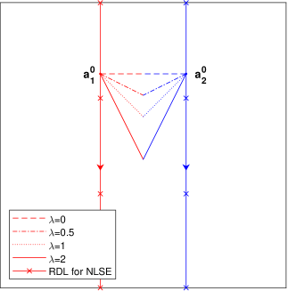
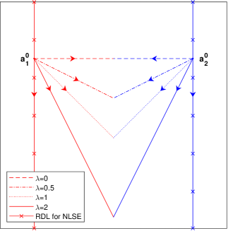
$(\alpha^{0},\beta^{0})=(-0.15,0.25)$	$(\alpha^{0},\beta^{0})=(-0.35,0.25)$

Figure 1: Some trajectories of some solution of (1.24) with different $\lambda$, the reduced dynamical laws of (1.7) (marked by “RDL for NLSE”) and the reduced dynamical laws of (1.8) (marked by “$\lambda=0$”) with initial data of the type (5.4).

Figure 1 shows some numerical results for the solution of (1.24) with initial data satisfying (5.5). It can be seen from Figure 1 that the trajectory of the solution of (1.24) converges to the trajectory of the solution of the reduced dynamical law of (1.8) as $\lambda\to 0$, and converges to the trajectory of the solution of the reduced dynamical law of (1.7) [13, 37] as $\lambda\to\infty$.

Lemma 5.3.

If $N=2$ and initial data (1.25) satisfies

$$\boldsymbol{a}^{0}_{1}=(0.5,0.5)^{T}+(\alpha^{0},\beta^{0})^{T},\quad\boldsymbol{a}_{2}^{0}=(0.5,0.5)^{T}+(-\alpha^{0},-\beta^{0}),$$ (5.12)

$$\boldsymbol{a}^{0}_{3}=(0.5,0.5)^{T}+(-\alpha^{0},\beta^{0})^{T},\quad\boldsymbol{a}_{4}^{0}=(0.5,0.5)^{T}+(\alpha^{0},-\beta^{0}),$$

then the solution $\boldsymbol{a}=\boldsymbol{a}(t)=(\boldsymbol{a}_{1}(t),\boldsymbol{a}_{2}(t),\boldsymbol{a}_{3}(t),\boldsymbol{a}_{4}(t))$ is of the following form

$$\boldsymbol{a}_{1}(t)=(0.5,0.5)^{T}+(\alpha(t),\beta(t))^{T},\quad\boldsymbol{a}_{2}(t)=(0.5,0.5)^{T}+(-\alpha(t),-\beta(t)),$$ (5.13)

$$\boldsymbol{a}_{3}(t)=(0.5,0.5)^{T}+(-\alpha(t),\beta(t))^{T},\quad\boldsymbol{a}_{4}(t)=(0.5,0.5)^{T}+(\alpha(t),-\beta(t)),$$

where $\alpha,\beta$ satisfy

$$\left(\begin{array}[]{c}\dot{\alpha}\\ \dot{\beta}\end{array}\right)=\frac{2}{1+\lambda^{2}}\left(\begin{array}[]{cc}1&\lambda\\ -\lambda&1\end{array}\right)\left(\begin{array}[]{c}\partial_{x}F(2\alpha,2\beta)-\partial_{x}F(2\alpha,0)\\ \partial_{y}F(2\alpha,2\beta)-\partial_{y}F(0,2\beta)\end{array}\right).$$ (5.14)

Proof.

The symmetry of initial data (5.12) and the symmetry of (1.24) imply that we can take the ansatz that the solution $\boldsymbol{a}$ satisfies (5.13). Substituting (5.13) into (1.24) and noting (5.10), (2.3), we have

$$\left(\begin{array}[]{cc}1&-\lambda\\ \lambda&1\end{array}\right)\dot{\boldsymbol{a}}_{1} =2(\nabla F(2\alpha,2\beta)-\nabla F(2\alpha,0)-\nabla F(0,2\beta))$$ (5.17)

$$=2\left(\begin{array}[]{c}\partial_{x}F(2\alpha,2\beta)-\partial_{x}F(2\alpha,0)\\ \partial_{y}F(2\alpha,2\beta)-\partial_{y}F(0,2\beta)\end{array}\right),$$ (5.20)

which together with (5.13) immediately implies (5.14). ∎

$(\alpha^{0},\beta^{0})=(-0.15,0.1)$	$(\alpha^{0},\beta^{0})=(-0.15,0.2)$
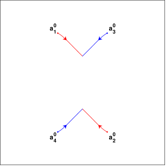
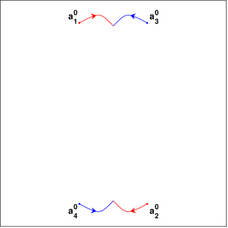
$(\alpha^{0},\beta^{0})=(-0.15,0.3)$	$(\alpha^{0},\beta^{0})=(-0.15,0.4)$
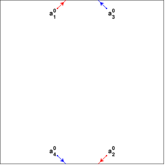
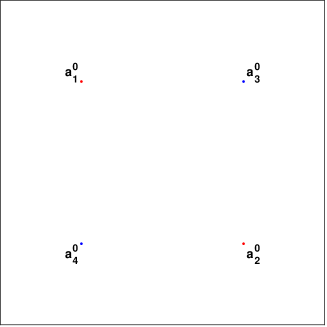
$(\alpha^{0},\beta^{0})=(-0.15,0.45)$	$(\alpha^{0},\beta^{0})=(-0.25,0.25)$

Figure 2: Some trajectories of solution of (1.24) with $\lambda=1$ and initial data satisfying (5.12).

Figure 2 shows some numerical results for the solution of (1.24) with $\lambda=1$ and initial data satisfying (5.5). The first five pictures in Figure 2 give five typical trajectories for fixed $\alpha^{0}$: (i) when $\beta^{0}$ is small, $\boldsymbol{a}_{1}$ will collide with $\boldsymbol{a}_{4}$ while $\boldsymbol{a}_{2}$ will collide with $\boldsymbol{a}_{3}$; (ii) as $\beta^{0}$ increases, $\boldsymbol{a}_{1}$ will get closer to $\boldsymbol{a}_{3}$, and if $\beta^{0}$ is large enough, $\boldsymbol{a}_{1}$ will collide with $\boldsymbol{a}_{3}$ while $\boldsymbol{a}_{2}$ will collide with $\boldsymbol{a}_{4}$; (iii) when $\beta^{0}$ is close to $0.5$ enough, $\boldsymbol{a}_{1}$ will collide with $\boldsymbol{a}_{4}$ again but in a direction different with the case (i). The last picture in Figure 2 gives an equilibrium state, which is caused by (5.9) and (5.10).

6 Conclusion

The reduced dynamical laws for quantized vortex dynamics of the complex Ginzburg-Landau equation on torus were established when the core size of vortex $\varepsilon\to 0$. The motion of vortices is governed by a mixed flow of gradient flow and Hamiltonian flow which are both driven by a renormalized energy on torus. Finally, a first integral of the reduced dynamical laws was presented and some analytical solutions with several initial setups with symmetry were obtained.

CRediT authorship contribution statement

Yongxing Zhu: Conceptualization, Methodology, Writing - original draft, Writing - review & editing.

Data availability

No data was used for the research described in the article.

Declaration of competing interest

The authors declare that they have no known competing financial interests or personal relationships that could have appeared to influence the work reported in this paper.

References

- [1] M. Aguareles, S. J. Chapman, T. Witelski, Interaction of Spiral Waves in the Complex Ginzburg-Landau Equation, Phys. Rev. Lett. 101(22) 224101.
- [2] M. Aguareles, S. J. Chapman, T. Witelski, Dynamics of spiral waves in the complex Ginzburg–Landau equation in bounded domains, Physica D 414 (2020) 132699.
- [3] I. S. Aranson, L. Kramer, The world of the complex Ginzburg-Landau equation, Rev. Mod. Phys. 74(1) (2002) 99–143.
- [4] W. Bao, Q. Du, Y. Zhang, Dynamics of rotating Bose-Einstein condensates and its efficient and accurate numerical computation, SIAM J. Appl. Math. 66 (2006) 758–786.
- [5] W. Bao, S. Shi and Z. Xu, Quantized vortex dynamics and interaction patterns in superconductivity based on the reduced dynamical law, Discret. Contin. Dyn. Syst. B 23 (2018) 2265–2297.
- [6] W. Bao, Q. Tang, Numerical study of quantized vortex interaction in the Ginzburg-Landau equation on bounded domains, Commun. Comput. Phys. 14(3) (2013) 819–850.
- [7] W. Bao, Q. Tang, Numerical study of quantized vortex interactions in the nonlinear Schrödinger equation on bounded domains, Multiscale Model. Simul. 12(2) (2014) 411–439.
- [8] F. Bethuel, H. Brezis, F. Helein, Ginzburg-Landau Vortices, Springer, Cham, 2017.
- [9] F. Bethuel, R. L. Jerrard, D. Smets, On the NLS dynamics for infinite energy vortex configurations on the plane, Rev. Mat. Iberoam. 24(2) (2008) 671–702.
- [10] F. Bethuel, G. Orlandi, D. Smets, Convergence of the parabolic Ginzburg–Landau equation to motion by mean curvature, Ann. Math. 163(1) (2006) 37–163.
- [11] G. P. Bewley, D. P. Lathrop, K. R. Sreenivasan, Visualization of quantized vortices, Nature 441(7093) (2006) 588–588.
- [12] K.-S. Chen, P. Sternberg, Dynamics of Ginzburg-Landau and Gross-Pitaevskii vortices on manifolds, Discret. Contin. Dyn. Syst. 34(5) (2014) 1905.
- [13] J. E. Colliander, R. L. Jerrard, Ginzburg-landau vortices: weak stability and schrödinger equation dynamics, J. Anal. Math. 77(1) (1999) 129–205.
- [14] Q. Du, L. Ju, Numerical simulations of the quantized vortices on a thin superconducting hollow sphere, J. Comput. Phys. 201(2) (2004) 511–530.
- [15] W. E, Dynamics of vortices in Ginzburg-Landau theories with applications to superconductivity, Physica D 77(4) (1994) 383–404.
- [16] P. C. Hohenberg, A. P. Krekhov, An introduction to the Ginzburg–Landau theory of phase transitions and nonequilibrium patterns, Phys. Rep. 572 (2015) 1-42.
- [17] R. Ignat, R. L. Jerrard, Renormalized energy between vortices in some Ginzburg–Landau models on 2-dimensional riemannian manifolds, Arch. Ration. Mech. Anal. 239(3) (2021) 1577–1666.
- [18] R. L. Jerrard, Vortex dynamics for the Ginzburg-Landau wave equation, Calc. Var. Partial Differ. Eqn. 9(1) (1999) 1–30.
- [19] R. L. Jerrard, H. M. Soner, Dynamics of Ginzburg‐Landau vortices, Arch. Ration. Mech. Anal. 142(2) (1998) 99–125.
- [20] R. L. Jerrard, D. Spirn, Refined Jacobian estimates and Gross–Pitaevsky vortex dynamics, Arch. Ration. Mech. Anal. 190(3) (2008) 425–475.
- [21] H. Y. Jian, Y. N. Liu, Ginzburg–Landau vortex and mean curvature flow with external force field, Acta Math. Sin. Engl. Ser. 22(6) (2006) 1831–1842.
- [22] M. Y. Kagan, Modern Trends in Superconductivity and Superfluidity, Springer, Dordrecht, 2013.
- [23] M. Kurzke, C. Melcher, R. Moser, D. Spirn, Dynamics for Ginzburg-Landau vortices under a mixed flow, Indiana Univ. Math. J. 58(6) (2009) 2597–2622.
- [24] F. H. Lin, Some dynamical properties of Ginzburg‐Landau vortices, Commun. Pure Appl. Math. 49(4) (1996) 323–359.
- [25] F. H. Lin, J. X. Xin, On the dynamical law of the Ginzburg-Landau vortices on the plane, Commun. Pure Appl. Math. 52(10) (1999) 1189–1212.
- [26] F. H. Lin, J. X. Xin, On the incompressible fluid limit and the vortex motion law of the nonlinear Schrödinger equation, Commun. Math. Phys. 200(2) (1999) 249–274.
- [27] E. Miot, Dynamics of vortices for the complex Ginzburg–Landau equation, Anal. PDE 2(2) (2009) 159–186.
- [28] P. Mironescu, On the stability of radial solutions of the Ginzburg-Landau equation, J. Funct. Anal. 130(2) (1995) 334–344.
- [29] S. Mowlaei, A. Roman, M. Pleimling, Spirals and coarsening patterns in the competition of many species: a complex Ginzburg–Landau approach, J. Phys. A: Math. Theor. 47(16) (2014) 165001.
- [30] J. C. Neu, Vortices in complex scalar fields, Physica D 43(2-3) (1990) 385–406.
- [31] L. P. Pitaevskii, Vortex lines in an imperfect Bose gas, Sov. Phys. JETP 13(2) (1961) 451–454.
- [32] J. Rubinstein, Self-induced motion of line defects, Q. Appl. Math. 49(1) (1991) 1–9.
- [33] E. Sandier, S. Serfaty, Gamma-convergence of gradient flows with applications to Ginzburg-Landau, Commun. Pure Appl. Math. 57(12) (2004) 1627–1672.
- [34] E. Sandier, S. Serfaty, A product-estimate for Ginzburg–Landau and corollaries, J. Funct. Anal. 211(1) (2004) 219–244.
- [35] S. Serfaty, Mean field limits of the Gross-Pitaevskii and parabolic Ginzburg-Landau equations, J. Am. Math. Soc. 30(3) (2017) 713–768.
- [36] Y. Zhang, W. Bao, Q. Du, Numerical simulation of vortex dynamics in Ginzburg-Landau-Schrödinger equation, Eur. J. Appl. Math. 18(5) (2007) 607–630.
- [37] Y. Zhu, W. Bao, H. Jian, Quantized vortex dynamics of the nonlinear Schrödinger equation on torus with non-vanishing momentum, (2023) arXiv:2304.02987.