Accurate and Definite Mutational Effect Prediction with Lightweight Equivariant Graph Neural Networks

Abstract

Directed evolution as a widely-used engineering strategy faces obstacles in finding desired mutants from the massive size of candidate modifications. While deep learning methods learn protein contexts to establish feasible searching space, many existing models are computationally demanding and fail to predict how specific mutational tests will affect a protein’s sequence or function. This research introduces a lightweight graph representation learning scheme that efficiently analyzes the microenvironment of wild-type proteins and recommends practical higher-order mutations exclusive to the user-specified protein and function of interest. Our method enables continuous improvement of the inference model by limited computational resources and a few hundred mutational training samples, resulting in accurate prediction of variant effects that exhibit near-perfect correlation with the ground truth across deep mutational scanning assays of 19 proteins. With its affordability and applicability to both computer scientists and biochemical laboratories, our solution offers a wide range of benefits that make it an ideal choice for the community.

1 Introduction

Mutation is a fundamental biological process that involves changes in the amino acid (AA) types of specific proteins. However, the functions of wild-type proteins may not always satisfy bio-engineering needs. Therefore, it is necessary to optimize their function, i.e., fitness, through favorable mutations. This operation is essential when designing antibodies (wu2019machine, ; pinheiro2021metabolic, ; shan2022deep, ) or enzymes (sato2019protein, ; wittmann2021advances, ). A protein typically consists of hundreds to thousands of AAs, where each belongs to one of the twenty AA types. To optimize a protein’s functional fitness, a greedy search is conventionally carried out in the local sequence. The process involves mutating AA sites to improve the functionality of the protein, rendering a mutant with a higher gain-of-function (rocklin2017global, ). Such a process is called directed evolution arnold1998design .

Obtaining mutants with high fitness requires mutating multiple AA sites of the protein, known as deep mutations (see Fig. 1). However, this process incurs significant experimental costs due to the astronomical number of potential mutation combinations. Thus, there is a need for in silico examination of protein variant fitness. A handful of deep learning methods have been developed to accelerate the discovery of advantageous mutants. For instance, Lu et al. lu2022machine applied 3DCNN to identify a new polymerase with a beneficial single-site mutation that enhanced the speed of degrading Polyethylene terephthalate (PET) by 7-8 times at 50${}^{\circ}\text{C}$. Luo et al. luo2021ecnet proposed ECNet to predict functional fitness for protein engineering with evolutionary context and guide the engineering of TEM-1 $\beta$-lactamase to identify variants with improved ampicillin resistance. Thean et al. thean2022machine enhanced SVD with deep learning in identifying Cas9 nuclease variants that possess higher editing activities than the derived base editors in human cells.

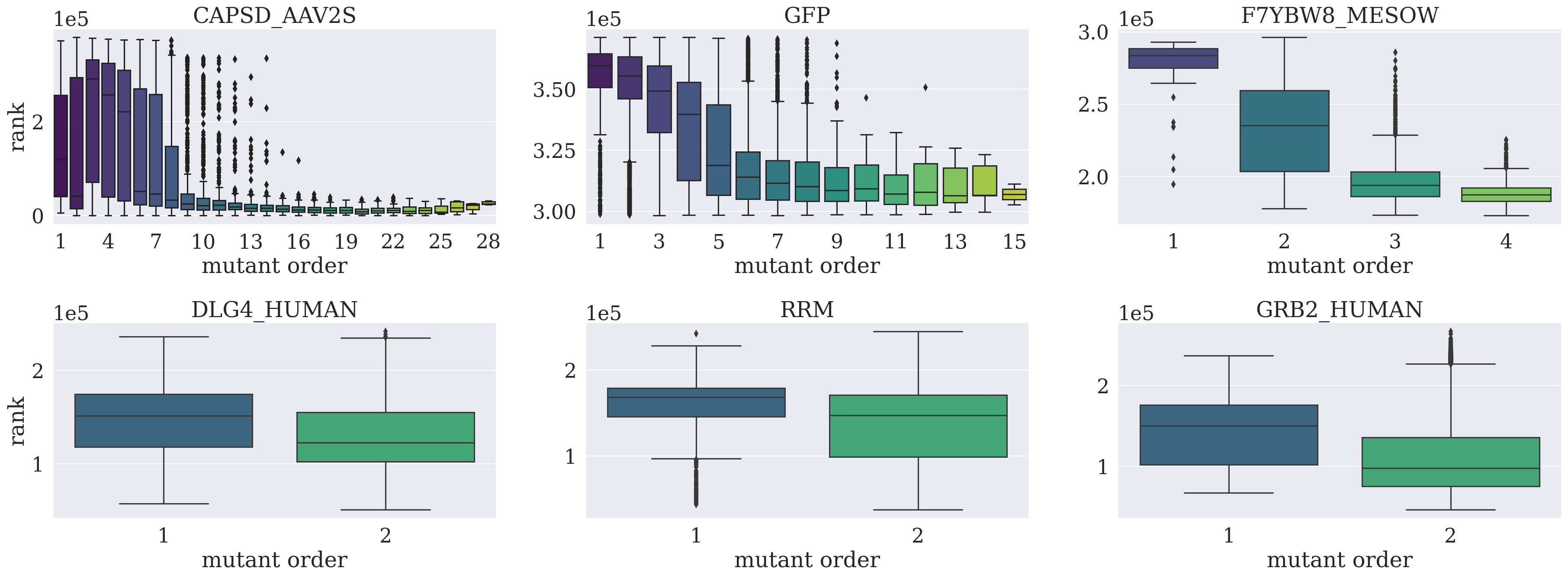
Figure 1: Mutating on more AA sites frequently results in better fitness, i.e., smaller average rank values.

The scarcity of labeled protein data and the uniqueness of distinct protein families make it challenging to train supervised learning models directly from observed mutants. As an alternative, researchers frequently pre-train models to encode protein sequences or structures and use the learned protein representations subsequently for specific tasks, such as de novo protein design from scratch (hsu2022esmif1, ), mutational effect prediction (ingraham2019generative, ; jing2020learning, ; meier2021esm1v, ; notin2022tranception, ), and higher-level structure prediction (ahmed2021protbert, ). This paper establishes a lightweight supervised learning strategy that trains on a few labeled protein data to suggest favorable mutational directions. Compared to existing methods that incrementally raise the prediction performance, our method is conceivably more suitable for guiding real scientific discovery. For instance, our method substantially surpasses one of the state-of-the-art models ESM-if1 hsu2022esmif1 on RRM for variant effects prediction. The ground-truth fitness score correlation of our method is higher than $0.9$, whereas the best obtained by ESM-if1 barely exceeds $0.4$.

Similar to training a novice in a new discipline, we maximize the learning efficiency of our proposed model by initially feeding it with a scalable dataset of wild-type proteins for context learning ahead of specifying proteins and functionalities. The pre-training process does not involve any supervision with real learning tasks or the target labels, and it is usually referred to as a self-supervised learning procedure. In literature, the problem is commonly reformatted to mini-de novo design that infers a specific AA type from its microenvironments, such as its neighboring AA types and local structure. Inferring optimal mutational directions from wild-type proteins can be viewed as a simulation of natural selection, given that mutation in natural conditions involves random changes of the AA type toward any of the other $19$ AA types. It is suggested by natural selection that only the mutants that exhibit optimal fitness and fit the environment survive. In computational algorithms, altering AA types of a wild-type protein can be viewed as adding corruptions to the node features of the protein graph, and recovering the perturbed graph becomes a remedy for identifying mutants with the best fitness. We thus model the protein mutation effect prediction as a denoising problem.

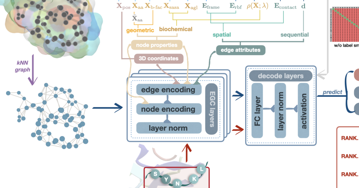
Figure 2: An illustration of the proposed method for variant effect predictions. (1) Data Preparation. An input graph is represented by a $k$NN graph with node and edge attributes of the corresponding AAs extracted from multiple scales, as well as nodes’ 3D positions. (2) Model Training. Wild-type protein graphs with noisy input attributes are fed to EGC layers for rotation and translation equivariant node embedding in the generic protein space. (3) Variant Effect Predictions. The fitness score of a mutant is derived from the joint distribution of the modified AA types on associated nodes. Updating the preliminary model with additional mutational samples can fit the specified protein and protein functionality better.

We provide a rich 3D spatial representation of the folded protein by a protein graph, where each AA corresponds to a node in the graph. The node features encode important information such as AA types, spatial coordinates of C$\alpha$, and C-N angles between neighboring AAs. The protein graph inputs are then processed by equivariant graph neural networks (EGNNs) (satorras2021n, ) in order to extract and utilize their geometric features in a rotationally-invariant manner. EGNNs provide a robust representation of AAs which are oriented differently depending on their location within the protein. It avoids costly data augmentation and leads to better performance in predicting mutations.

Our proposed model is lightweight since it begins with encoding proteins’ structural and biochemical properties using a few layers of graph convolutions. The training precludes multiple sequence alignment (MSA) (riesselman2018deep, ; frazer2021disease, ; rao2021msa, ) and protein language models (ahmed2021protbert, ; rives2021biological, ; nijkamp2022progen2, ; brandes2022proteinbert, ), both of which require substantial computational resources, such as hundreds of GPU cards, and massive data mining from millions of proteins. The high demand for computing resources hinders model revisions for the former approach, while the latter requires evolutionary properties of the protein family and considerable amounts of high-quality protein data for effective training.

Furthermore, our method circumvents the assumption of independent mutations in predicting the fitness of higher-order mutations by considering the joint distribution of AAs across the entire protein sequence. Traditional approaches that arrange autoregressive inference processes to find the conditional score for individual mutations at a single site are not only time-consuming for lengthy proteins but also based on an incorrect assumption that mutations on different sites occur sequentially or independently. The trivial assumption ignores epistatic effects among different sites, which are considered crucial factors in finding favorable high-order mutations, thus hindering directed evolution (sato2019protein, ; liu2022rotamer, ; hsu2022esmif1, ; notin2022tranception, ).

To summarize, the proposed lightweight equivariant graph neural network (LGN) has distinct advantages for predicting variant effects from three perspectives. First and foremost, it enables instant and highly reliable deep mutational effect inference that is specific to the protein and functionality. Secondly, the model is capable of generalizing to unseen proteins, making it a useful tool for recommending directional evolution strategies. Furthermore, LGN circumvents the independent-mutation assumptions and instead incorporates epistatic effects by utilizing the joint distribution of all variations. Empirically, we test LGN on $19$ proteins of up to 28-site mutations. On average, our model reaches $0.841$ Spearman’s correlation in deep mutational effect predictions. It has outperformed the other supervised model ECNet luo2021ecnet by $4.7\%$, and the rest SOTA self-supervised baseline models (e.g., DeepSequence (riesselman2018deep, ) and ESM-IF1 (hsu2022esmif1, )) by $83.3\%$.

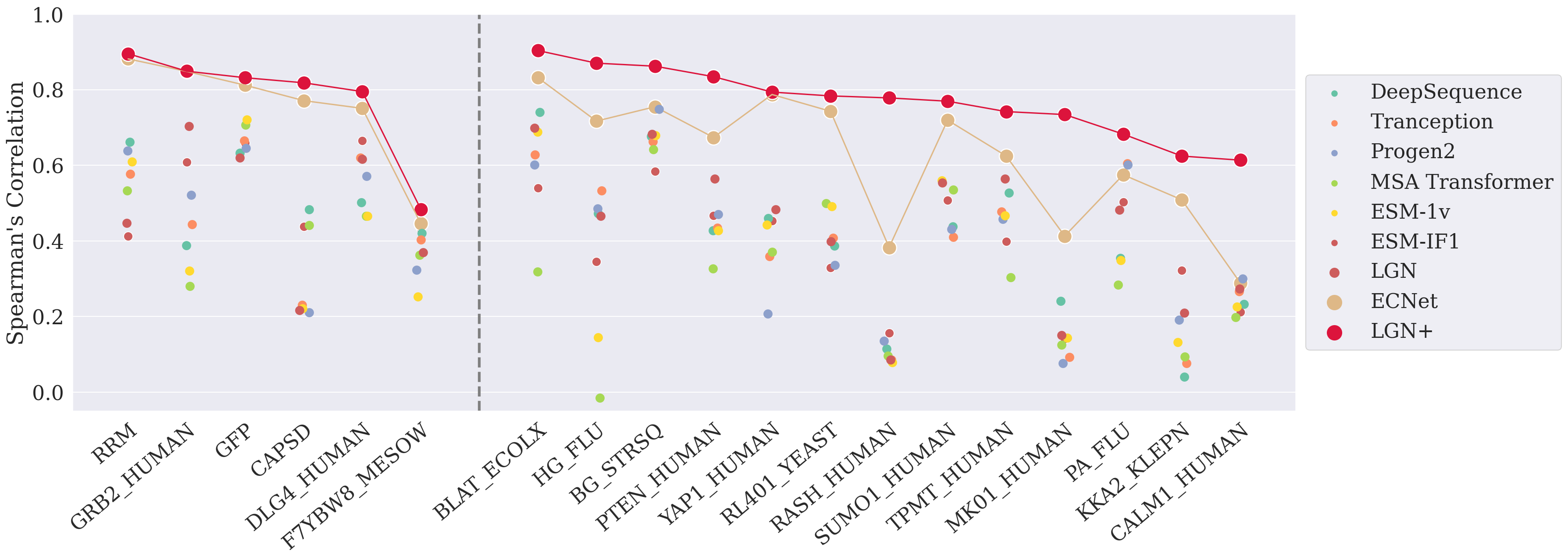
Figure 3: Per task performance on the variant effect prediction with models trained from zero-shot and supervised learning tasks. Colored scatters indicate Spearman’s correlation coefficients on the corresponding protein achieved by different models. The left $6$ proteins contain higher-order mutations, and the right $13$ proteins record shallow mutants.

2 Results

The ability of LGN to predict variant effects is evaluated with deep mutational scanning (DMS) assays fowler2014deep , which provides a systematic survey of the mutational landscape of proteins from wet-lab tests and is commonly used to benchmark computational predictors’ effectiveness for evaluating mutations. Fig. 2 displays the overall workflow of our model, where a protein graph with attributed nodes and edges (see construction rules in Section 3.1) is inputted into equivariant graph convolutional layers to obtain appropriate node embeddings, which will be decoded for label prediction.

2.1 Fitness of Deep Mutations Prediction

Our model predicts the fitness scores following two different routes, depending on whether protein-specific true scores are available. If there is no access to additional mutations, our model directly provides a preliminary assessment based on observations from nature and takes the log-odds-ratio from the predicted probabilistic distribution of the mutations. When a small set of mutations is available, the model will first be fine-tuned to predict accurate fitness scores of the underlying protein. The two models, without and with fine-tuning steps, are named LGN and LGN+, respectively. The fitness score provides an overall assessment of the measurable characteristics of a protein in relation to specified mutations, such as enzyme function, growth rate, peptide binding, viral replication, and protein stability. A higher fitness score indicates that the mutant benefits from certain adjustments of associated sidechain types.

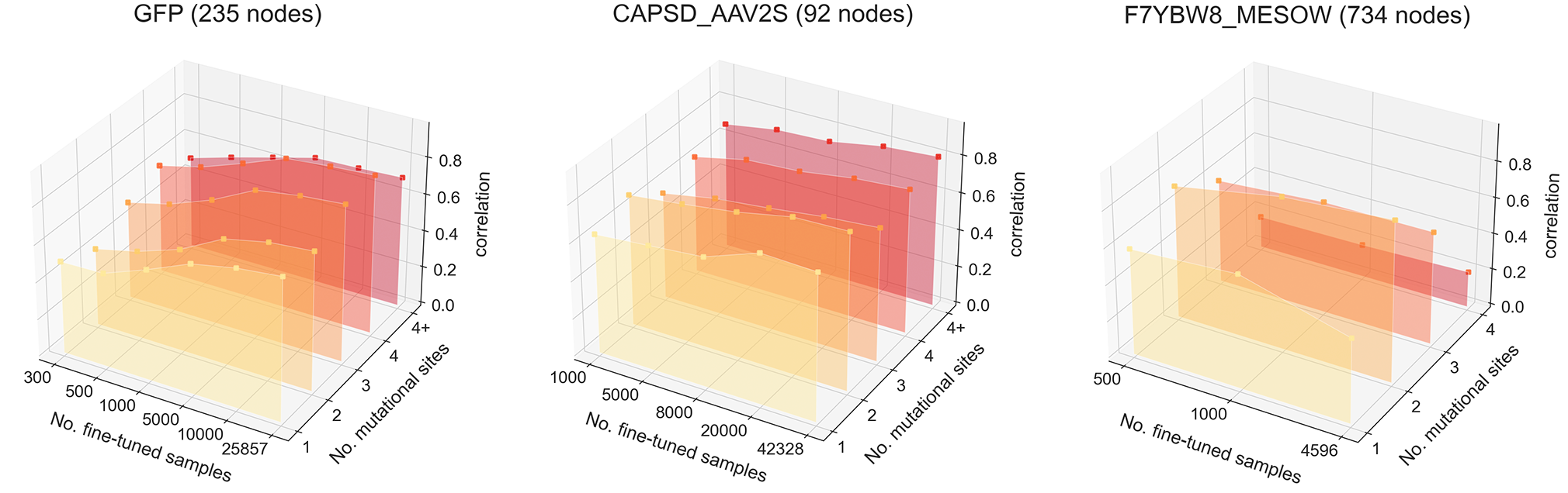
Figure 4: A small fraction of wet-lab test results are sufficient for greatly boosting LGN’s prediction performance.

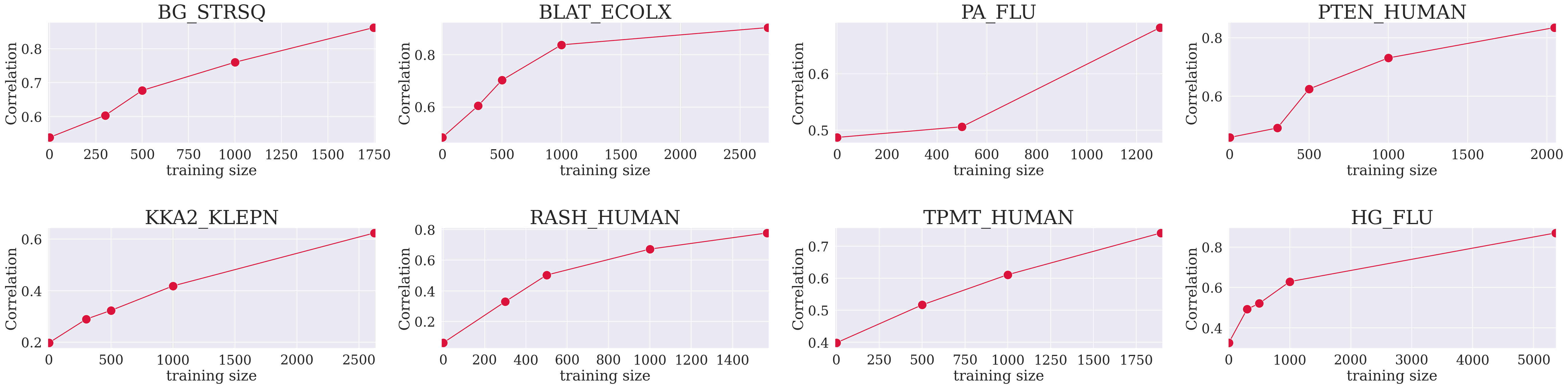
Figure 5: The Spearman’s Correlation of fitness prediction on single-site mutations with different numbers of training samples.

The comparison of LGN’s performance is made with seven state-of-the-art baseline models on $299,120$ mutants from $19$ DMS experiments that cover $1$-site to $28$-site mutation scores in literature, where $13$ of them only mutate on single sites, and the rest $6$ of them test DMS assays on both single site and higher-order sites. To evaluate the reliability of variant effect predictions, we calculate protein-wise Spearman’s correlation coefficient between the computational and experimental scores. The results are visualized in Fig. 3. The preliminary LGN achieves comparable performance among other competitors, and minimum efforts advance LGN+ (denoted by the threaded crimson bullets $\bullet$) to substantially lead other competitors on different proteins. The enhanced LGN+ not only requires little computational resources but also consumes limited scored mutational samples to significantly improve the prediction performance. The number of fine-tuned samples for promising performance is investigated in Fig. 4 and Fig. 5 for multiple-sites and single-site mutational predictions. It turns out that a few hundred can boost the correlation score, and up to thousands of mutational scores are sufficient for achieving a prominent correlation score even in the case of deep mutates.

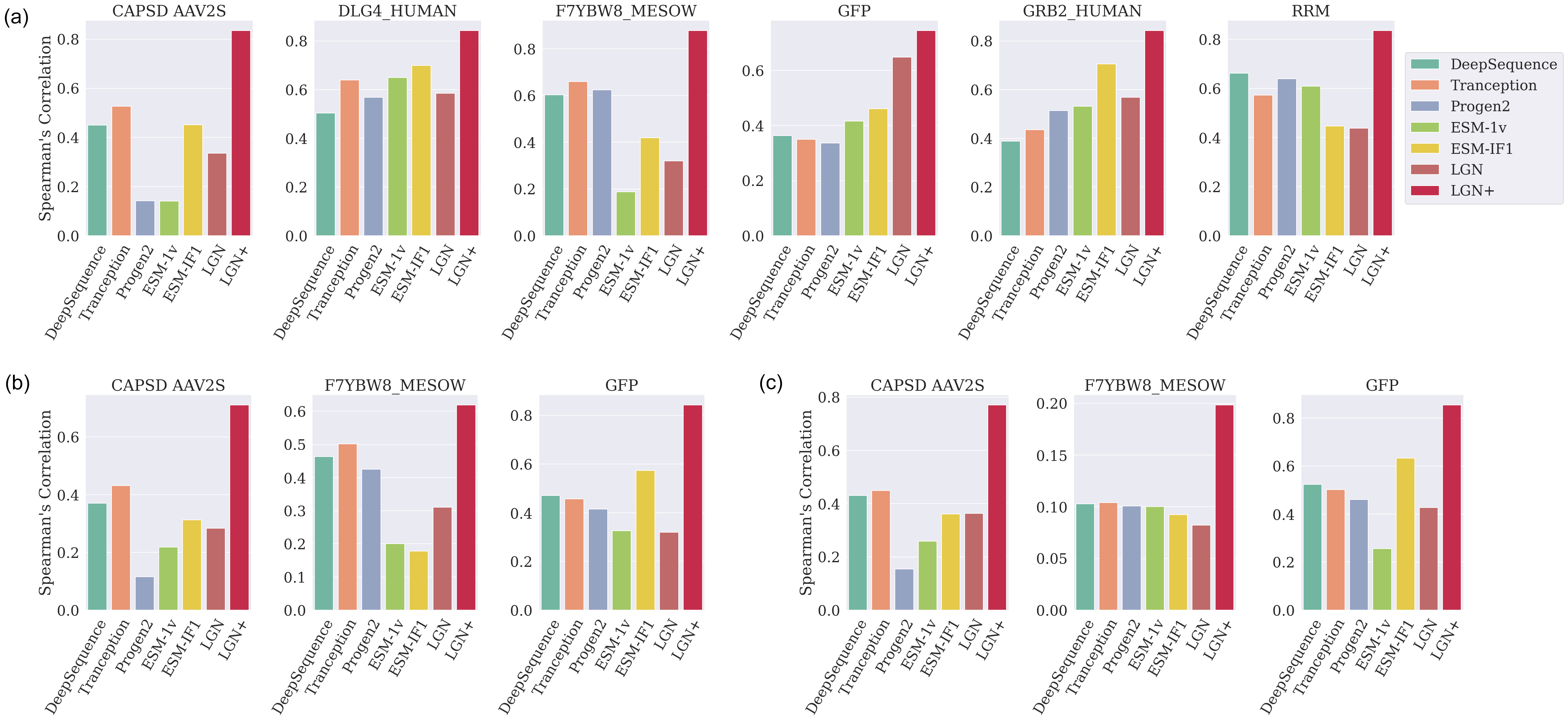
Figure 6: The Spearman’s Correlation of fitness prediction on deep mutations. The three subplots (a), (b), and (c) are with respect to 2, 3, and 4-order mutations.

Table 1: Spearman’s correlation and True positive rate (TPR) comparison of ECNet and LGN+ on the $13$ proteins of single-site mutations.

	Spearman’s Corr.		TPR (20%)
protein	ECNet	LGN	ECNet	LGN
BLAT_ECOLX	$0.832$	$0.903$	$0.586$	$0.728$
HG_FLU	$0.717$	$0.870$	$0.593$	$0.759$
BG_STRSQ	$0.755$	$0.862$	$0.758$	$0.805$
PTEN_HUMAN	$0.674$	$0.834$	$0.479$	$0.699$
YAP1_HUMAN	$0.787$	$0.794$	$0.676$	$0.743$
RL401_YEAST	$0.743$	$0.783$	$0.421$	$0.603$
RASH_HUMAN	$0.383$	$0.778$	$0.333$	$0.557$
SUMO1_HUMAN	$0.719$	$0.769$	$0.535$	$0.688$
TPMT_HUMAN	$0.625$	$0.742$	$0.435$	$0.611$
MK01_HUMAN	$0.413$	$0.734$	$0.337$	$0.293$
PA_FLU	$0.575$	$0.682$	$0.306$	$0.470$
KKA2_KLEPN	$0.509$	$0.624$	$0.588$	$0.648$
CALM1_HUMAN	$0.289$	$0.614$	$0.278$	$0.607$

Fig. 6 details the evaluations on protein-specific and order-specific fitness prediction. Based on the available experimental records, the number of mutational sites is designated to 2-4 on the six proteins that explored deep mutational effects. It can be seen that LGN+ champions higher-order mutations by up to over 100% improvement. The beneficial supervision of new experimental data is backed up by the lightweight model architecture of LGN, which is an advanced property that is exclusive to LGN. A comprehensive comparison of the training and inference cost is discussed in Section 2.4.

We also compare the two supervised learning models, ECNet and LGN+, by Spearman’s correlation and true positive rate (for the top 20%-ranked mutations) for single-site shallow mutations. Both methods take $10\%$ of the total records for training. According to the results reported in Table 1 and Fig. 3, LGN+ outperforms ECNet steadily and significantly on both metrics in predicting single-order mutational effects. This could be explained by the fact that ECNet, as a completely supervised model, requires more training data to achieve satisfactory prediction performance. Since generating mutational effect data through wet labs is usually expensive and time-consuming (due to the technical difficulties and the slow turnaround time of conducting experiments), it is desirable to tune a high-performance model with minimal supervision or with a small training set.

2.2 Enhance Protein Embedding with Prior Knowledge

To encourage the network to capture essential protein features, we integrate various types of prior knowledge into our pre-training procedure. Specifically, we incorporate perturbations on amino acid (AA) types to simulate potentially harmful mutations in wild-type proteins liu2022rotamer . We also implement substitution matrices for noise generation and label smoothing to assist the generated mutations in accurately reflecting the natural variation.

AA Type Denoising

We refine the AA type of a node ${\bm{x}}_{\text{aa}}$ to $\tilde{{\bm{x}}}_{\text{aa}}$ with a Bernoulli noise, i.e.,

$$\bm{\pi}(\tilde{{\bm{x}}}_{\text{aa}}\mid{\bm{x}}_{\text{aa}})=p\delta(\tilde{{\bm{x}}}_{\text{aa}}-{\bm{x}}_{\text{aa}})+(1-p)\bm{\Theta}(\pi_{1},\pi_{2},\dots,\pi_{20}),$$ (1)

where the confidence level $p$ is a tunable parameter that controls the proportion of residues that are considered to be ‘noise-free’. It can also be determined by prior knowledge regarding the quality of wild-type proteins, i.e., how frequently are mutations expected to happen in nature. For example, a value of $p=1$ indicates the maximum confidence in wild-type protein quality, which results in no perturbations to the input AA.

The probability for the residue to become a particular type depends on the defined distribution $\bm{\Theta}$. A naive choice for $\bm{\Theta}$, the expected frequency distribution of AA types, is setting them to equal values: $\pi_{1}=\pi_{2}=...=\pi_{20}=0.05$, although it could be informed by prior knowledge based on molecular biology with the observed probability density of AA types in wild-type proteins. Substitution matrices can be another choice for defining pair-wise exchange probabilities while helping with robust representation learning through the use of label smoothing techniques.

Figure 7: Average Performance with different $p$s on various AA noises (row) and mutational numbers. We use ‘mutate type=single’ to indicate shallow 1-site mutations, and ‘mutate type=multiple’ for deep mutations.

We evaluate the performance of the model with the above three types of exchange distributions $\bm{\Theta}$, as shown in Figure 7. It examines the sensitivity of $p$’s choices by the average Spearman’s correlation under different AA noise distributions, including random uniform distribution, wild-type AA distribution, and the substitution matrix. We are examining the general scenario where none of the mutants have undergone labeling or testing in wet labs. We have excluded extremely small values of $p$ to prevent drastic perturbation rates and to facilitate the search for an optimal $p\in\{0.3,0.4,\dots,0.9,1\}$. Different choices on $p$s are validated with three different learning tasks, which will be introduced shortly in Section 2.3. A sharp decrease at $p=1$ certifies the effectiveness of introducing perturbations on AA types to the performance improvement of fitness prediction on both single-site and multiple-site mutations. Also, incorporating affinity learning tasks alongside AA sequence prediction facilitates the generation of more expressive node embeddings, as evidenced by the superior zero-shot fitness prediction performance. Notably, the prediction of SASA for each node using hidden protein graph embeddings yields significant enhancements compared to AA-only learning tasks. While including the additional B-factor predictor does not see significant advances on top of SASA prediction, it perfects the optimal model with better performance. In general, assigning a moderate value to $p$ between $0.4$ and $0.7$ is suitable for different combinations of learning modules and noise distributions. Based on the overall performance, we have set the default value of p to 0.6 as the confidence level for our model.

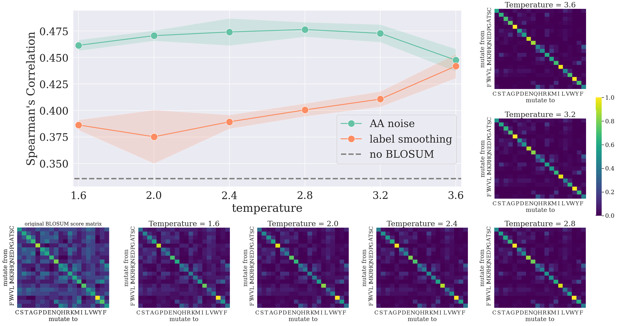
Figure 8: Average Spearman’s correlation over $5$ repetitive runs on deep mutations with different temperatures on the BLOSUM62 matrix, where the matrix is used for generating AA noise (in orange) or label smoothing (blue). The normalized BLOSUM62 matrices as well as the original matrix are visualized at different temperature levels.

Label Smoothing with Amino Acid Substitution Matrices

Protein sequence alignments provide important insights for understanding gene and protein functions. The similarity measurement of a protein sequence alignment reflects the favors of all possible exchanges of one AA over another. We employ BLOSUM62 substitution matrix (henikoff1992amino, ) to account for the relative substitution frequencies and chemical similarity of AAs. The matrix is derived from the statistics for every conserved region of protein families in BLOCKS database. Given that AA sites are more likely to mutate to AA types with high similarity scores in the BLOSUM62 table, we used this matrix to modify our loss function with the label smoothing technique. Specifically, mutations to AA types with higher similarity scores accumulate smaller penalties compared to those with lower similarity scores.

Fig. 8 demonstrates the modified BLOSUM62 matrix with different temperatures for defining the label smoothing and perturbation probability. The temperature $t$ is introduced to control the degree of dispersion towards off-diagonal regions, which transforms the substitution matrix ${\bm{B}}$ to ${\bm{B}}^{\prime}$ by ${\bm{B}}^{\prime}=\sigma({\bm{B}})^{t}$, where $\sigma(\cdot)$ is a non-linear operator, such as normalization. Intuitively, increasing $t$ pushes ${\bm{B}}$ towards a diagonal matrix, and it is agnostic to a higher confidence level $p$ in wild-type noise, in the sense that both of them return more diagonal-gathered substitution matrices. The line plot reports the average correlation (over $5$ repetitive runs) of variant effect predictions for the $6$ deep mutational proteins with $p=0.6$. Compared to the baseline results of random AA noise and no label smoothing, applying the BLOSUM62 matrix to either AA noise or label smoothing improves the predictions. Overall, a higher temperature for the label smoothing matrix yields better overall performance, while a moderate temperature that produces more nuanced noise to AA types is preferred.

2.3 Multitask Learning Strategy

We utilize the multitask learning approach for the self-supervised learning module to enhance the microenvironment embedding of AAs and advance the expressivity of the hidden node representation.

Initially, the model corrects the perturbed AA types and predicts the joint distribution of the types of all AAs, i.e., ${\bm{y}}_{aa}\in\mathbb{R}^{20}$. Concurrently, additional auxiliary tasks that predict ${\bm{y}}_{\text{sasa}}$ and ${\bm{y}}_{\text{B-fac}}$ introduce inductive biases to enhance the model’s predictive capabilities. The former property, SASA, strongly influences AA type preferences, and the latter, B-factor, is associated with the conformations and mobility of the neighboring AAs. Both properties are closely connected to AAs and are essential in describing an underlying AA. Predicting the two features is thus beneficial, allowing the implicit encoding of the features without the risk of data leakage.

The efficacy of incorporating both auxiliary tasks has been previously examined in Fig. 7. The results demonstrate that including these supplementary targets significantly enhances performance, regardless of the selected noise distribution. Moreover, Fig. 9 indicates that all three tasks are well-learned during pre-training by reporting the predicted ${\bm{y}}$s. Specifically, the confusion matrix of the predicted AA types with respect to the ground-truth AA types is visualized to assess the model’s ability to recover from noisy sequences to the original sequence. The vast majority of predictions accumulating on the diagonal line indicate a high recovery rate with respect to AA types. For the two regression tasks, i.e., SASA and B-factor predictions, we used linear regression to fit the true value against the predicted value, yielding estimated coefficients of $0.989$ and $1.008$, respectively, while both the corresponding $p$-values were found to be $<0.001$. Pearson’s correlation coefficients for the predicted and true values of the two features are fairly high at $0.884$ and $0.791$, respectively.

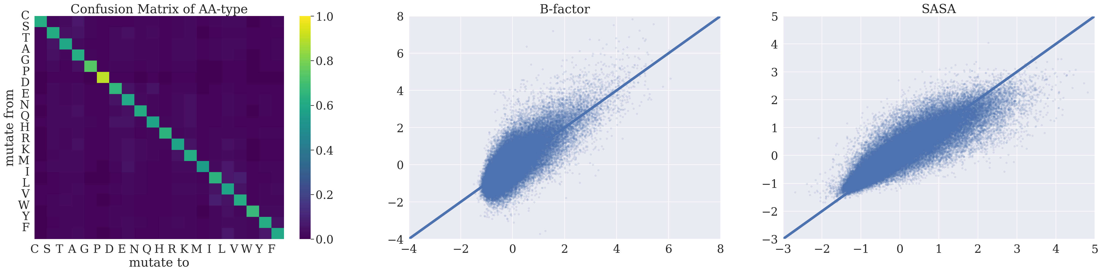
Figure 9: Confusion matrix of predicted AA types (left), and linear regression on the predicted SASA (middle) and B-factor (right).

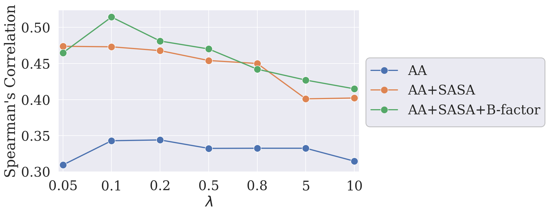
Figure 10: The influence of $\lambda$ on the loss of predicting ${\bm{y}}_{\text{sasa}}$ and ${\bm{y}}_{\text{B-fac}}$ to the overall correlation.

It is crucial to balance the attention assigned to the three learning tasks and control their contribution to the overall prediction error ${\mathcal{L}}_{\text{total}}={\mathcal{L}}_{\text{aa}}+\lambda_{1}{\mathcal{L}}_{\text{sasa}}+\lambda_{2}{\mathcal{L}}_{\text{B-fac}}$ with factors $\lambda_{1},\lambda_{2}$. Here we investigate a wide range of the choices of $\lambda$s to the impact of model training. As both ${\bm{y}}_{\text{sasa}}$ and ${\bm{y}}_{\text{B-fac}}$ share a consistent value scale, we let $\lambda_{1}=\lambda_{2}\in\{0.05,0.1,0.2,0.5,0.8,5,10\}$. We conducted all experiments with wild-type noise and set $p=0.6$. The average Spearman’s correlations, reported in Fig. 10, exhibit an overall decreasing trend, highlighting the importance of accurately predicting ${\bm{y}}_{\text{aa}}$ as the primary objective for the model. The scores corresponding to $\lambda$ values from $0.05$ to $0.1$ indicate that including the two auxiliary tasks is necessary, particularly when making all three predictions simultaneously. Furthermore, the overall trend suggests that accurately predicting ${\bm{y}}_{\text{aa}}$ remains the model’s primary objective. Notably, there is a small peak in the scores between $\lambda=0.1$ and $\lambda=0.2$, implying that smaller values of $\lambda$ are generally preferable.

2.4 Training Cost of Self-Supervised Models

Introducing abundant prior domain knowledge not only let LGN achieve excellent performance in variant effects prediction tasks with interpretable designs, but also significantly reduced the computational resources required during both model training and inference. The former advantage of eased and faster network training is particularly favored for instant model optimization and modification on specific proteins or directed evolution targets.

Fig. 11 and Table 2 deliver a direct comparison of our model against the baseline methods with respect to the model scale, inference time, and prediction performance. As the majority of models are pre-trained, we record the inference speed on a single NVIDIA GeForce RTX 3090. Note that the inference time varies with the length of the protein sequence and the size of the test set, we thus take an example protein GFP that consists of $236$ AA residues and has evaluation scores on over $50,000$ mutants for testing. Although all these in silico computational costs are significantly lower than wet lab tests, we use the inference time to indicate the cost of forward propagation in one iteration, which is proportional to the model scale. In terms of ECNet, the running time also depends on the number of available training samples and the highest number of mutational orders. In the case of GFP, it takes $8,280$ seconds to finish the training procedure on around $5,200$ mutants (i.e., $10\%$ of the total DMS samples).

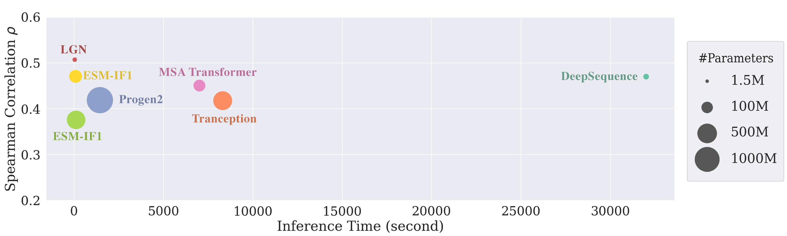
Figure 11: Comparison of Inference Efficiency on pre-trained models. The area of the ball indicates the number of network parameters of a model. Our model (in blue) can achieve SOTA performance ($y$-axis) with minimum inference time ($x$-axis) and $1\%$ number of parameters of the ESM.

Table 2: Comparison of baseline zero-shot pre-trained models. The train and inference speed is tested on GFP.

model	DeepSequence	MSA Trans.	ESM-1v	ESM-IF1	Tranception	ProGen2	LGN (ours)
input	sequence	sequence	sequence	sequence+structure	sequence	sequence	structure
MSA	$\checkmark$	$\checkmark$			$\checkmark$
train on new protein	$\checkmark$				$\checkmark$
training dataset	-	Uniref50	Uniref90	CATH+AF2	Uniref100	Uniref90+BFD30	CATH
	-	(2018-03)		(2020-03)			v4.3.0
training size (M)	-	$45$	$98$	$12$	$249$	$>1,000$	$0.03$
max. input token		$1,024$	$1,024$	$1,024$	$1,280$	$1,024$	$2,687^{\dagger}$
# parameters (M)	$4.3$	$100$	$650$	$142$	$700$	$2,700$	$1.5$
# layers	$1,600$	$12$	-	$20$	$36$	$32$	$6$
# head	-	$12$	-	$8$	$20$	$32$	-
# hid. dim.	$100-2,000$	-	-	$512-2,048$	-	-	$512$
speed (training day)	-	$13^{\dagger\dagger}$	$6$	$653$	$\sim$100	-	$0.17$
resource (train)	-	128$\times$V100††	64$\times$V100	32$\times$V100	64$\times$A100	?$\times$TPU-v3	1$\times$3090
preparing speed (sec)	$6,360+25,020$	$6,360$	-	-	$6,360$	-	-
inference speed (sec)	$608$	$927$	$75$	$102$	$1,920$	$1,440$	$25$
$\dagger$ The $2,687$ input token length only refers to the maximum protein length we used during training, rather than its maximum capacity.
$\dagger\dagger$ The training speed and required resources are retrieved from meier2021esm1v .

3 Methods

When designing an expressive geometric deep learning model for predicting DMS assays on proteins, two principles should be carefully considered. Firstly, based on the laws of physics, the atomic dynamics of proteins remain unchanged, regardless of their translation or rotation from one position to another.(han2022geometrically, ). Therefore, the inductive bias of symmetry should be incorporated into the design of protein structure-based models. This ensures that the spatial relationship of AAs (torng20173d, ; sato2019protein, ) or geometric equivariance (ganea2021independent, ; stark2022equibind, ) are respected. Second, a protein encoder that is both expressive and general is required to balance the conflicts between scarce mutational records and the substantial resources required to train representation learning models. As with many studies (ahmed2021protbert, ; zhang2022protein, ; hsu2022esmif1, ; castro2022transformer, ), this work starts from a self-supervised method for discovering expressive representation for the rational protein space. On the contrary to related works in literature, we did not employ multiple sequence alignment (MSA) riesselman2018deep ; jumper2021highly ; rao2021msa ; wang2022lm . This is because not all proteins are alignable (such as CDR regions of antibody variable domains (shin2021protein, )) and not all the alignments are deep enough to train models sufficiently large capable of learning the complex interactions between residues. Instead, we approach fast and robust modeling with proteomic knowledge and multitask learning strategies. When there are additional experimental records, the constructed model can be revised in the later stage.

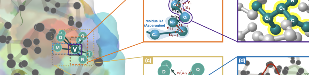
Figure 12: Illustrative node and edge features of a protein graph (PDB ID: 1KDF). For a particular node V45, i.e., Valine at position 45: (a) the dihedral angle and local frames are constructed by the positions of the heavy atoms of V45 and N46 (the next residue on the sequence), where the local frames are also used for generating neighboring projections for edge features; (b) the AA type, B-factor, and SASA are generated from the raw .pdb input; (c) the surface-aware features describe the weighted sum force of 1-hop neighbors, and the scale of this force implies whether it’s an interior or surface-closed AA; (d) sequential relative positions and contact indicators are encoded in the edge attributes of connected nodes.

3.1 Graph Representation of Folded Proteins

The geometry of proteins suggests higher-level structures and topological relationships, which are vital to protein functionality. For a given protein, we create a $k$-nearest neighbor ($k$NN) graph ${\mathcal{G}}=({\bm{X}},{\bm{A}},{\bm{E}})$ to describe its 3D structure and molecular properties. Here each node represents an AA with ${\bm{X}}\in\mathbb{R}^{36}$ node attributes describing $21$ biochemical and $15$ geometric properties of AAs. The edge connections are formulated by a symmetric adjacency matrix ${\bm{A}}$ with the $k$NN-graph to capture the nodes’ microenvironment, i.e., each node is connected to up to $k$ other nodes in the graph that has the smallest Euclidean distance over other nodes, and the distance is smaller than a certain cutoff (e.g., $30\AA$). Consequently, if node $i$ and $j$ are connected to each other, we have ${\bm{A}}_{ij}={\bm{A}}_{ji}\neq 0$ with edge features ${\bm{E}}\in\mathbb{R}^{93}$ defined on them. We now introduce the node and edge features.

The biochemical node features include $20$ one-hot encoded AA types (${\bm{X}}_{\text{aa}}$) and a scalar value, i.e., the standardized crystallographic B-factor, that identifies the rigidity, flexibility, and internal motion of each residue. Note that the raw B-factor is sensitive to the experimental environment and proteins in our dataset are measured by different laboratories, therefore we decide to fix the measurement bias by taking standardized B-factors along each protein. Specifically, we standardize the raw B-factor values with AA-wise mean and standard deviation.

Regarding the geometric node attributes, we include solvent-accessible surface area (SASA), normalized surface-aware node features, dihedral angles of backbone atoms, and 3D positions. SASA measures the level of exposure of an AA to solvent in a protein, which provides an important indicator of active sites of proteins to locate whether a residue is on the surface. The $5$ mean force features implement a non-linear projection to the weighted average distance of a residue to their one-hop neighbors $i^{\prime}\in\mathcal{N}_{i}$, i.e.,

$$\rho\left(\mathbf{x}_{i}\mathchar 24635\relax\;\lambda\right)=\frac{\left\|\sum_{i^{\prime}\in\mathcal{N}_{i}}w_{i,i^{\prime},\lambda}\left({\bm{X}}_{\text{pos},i}-{\bm{X}}_{\text{pos},i^{\prime}}\right)\right\|}{\sum_{i^{\prime}\in\mathcal{N}_{i}}w_{i,i^{\prime},\lambda}\left\|{\bm{X}}_{\text{pos},i}-{\bm{X}}_{\text{pos},i^{\prime}}\right\|},$$

where the weights are defined by $w_{i,i^{\prime},\lambda}=\frac{\exp\left(-\left\|{\bm{X}}_{\text{pos},i}-{\bm{X}}_{\text{pos},i^{\prime}}\right\|^{2}/\lambda\right)}{\sum_{i^{\prime}\in\mathcal{N}_{i}}\exp\left(-\left\|{\bm{X}}_{\text{pos},i}-{\bm{X}}_{\text{pos},i^{\prime}}\right\|^{2}/\lambda\right)}$ with $\lambda\in\{1,2,5,10,30\}$. These features describe whether the node is on the surface of the protein. A surface-closed AA with neighbors from a narrower range leads to larger feature values and stronger mean forces ganea2021independent . The ${\bm{X}}_{\text{pos},i}\in\mathbb{R}^{3}$ denotes the 3D coordinates of the $i$th residue, which is represented by the position of $\alpha$-carbon. Moreover, the spatial conformation of the AA in the protein chain is measured by ${\bm{X}}_{\text{agl},i}\in\mathbb{R}^{6}$, which contains the trigonometric values of dihedral angles $\{\sin,\cos\}\circ\{\phi_{i},\psi_{i},\omega_{i}\}$ of the backbone atom positions. The three dihedral angles $\phi_{i},\psi_{i}$, and $\omega_{i}$ describe the torsion angle between the heavy atoms $N_{i}-C\alpha_{i},C\alpha_{i}-C_{i}$, and $C_{i}-N_{i+1}$. The last nodes of AA sequences are removed to avoid inaccessible angles.

The edge attributes ${\bm{E}}\in\mathbb{R}^{93}$ feature the connected edges in the graph, including $15$ high-dimensional distances, $12$ relative spatial positions, and $66$ relative sequential distances. For two connected residues $i$ and $j$, the distance between them is projected by Gaussian radial basis functions (RBF), i.e.,

$${\bm{E}}_{r}^{\rm rbf}({\bm{x}}_{i},{\bm{x}}_{j})=\exp\left\{\frac{\|{\bm{x}}_{j}-{\bm{x}}_{i}\|^{2}}{2\sigma^{2}_{r}}\right\},\quad r=1,2,\dots,R.$$

A total number of $15$ distinct distance-based features are created on the edge with the scale parameter $\sigma_{r}=\{1.5^{k}\mid k=0,1,2,\dots,14\}$. From the corresponding residues’ heavy atoms positions, the two local frames define $12$ relative positions ganea2021independent of node $j$ with respect to node $i$. They represent local fine-grained relations between AAs and the rigid property of how the two residues interact with each other. Finally, the residues’ sequential relationship is encoded with $66$ binary features by their relative position $d_{i,j}=|s_{i}-s_{j}|$, where $s_{i}$ and $s_{j}$ are the absolute positions of the two nodes in the AA chain. For instance, if $v_{i}$ is the first AA in the sequence and $v_{j}$ is the fifth AA, we have $s_{i}=1$ and $s_{j}=5$. We set a cutoff at $64$, i.e., $d_{i,j}=\min(|s_{i}-s_{j}|,65)$ based on the fact that the locally connected nodes (by the $k$NN defined edges) merely have their positional distance over $64$ and transform this distance feature with one-hot encoding liu2022rotamer . In addition, we define a binary contact signal ${\bm{E}}_{\text{contact}}$ ingraham2019generative to indicate whether two residues contact in the space, i.e., the Euclidean distance $\|C\alpha_{i}-C\alpha_{j}\|<8$.

3.2 Equivariant Protein Graph Convolution

Bio-molecules such as proteins and chemical compounds are structured in the 3-dimensional space, and it is vital for the model to predict the same binding complex no matter how the input proteins are positioned and oriented. Instead of practicing expensive data augmentation strategies, we construct SE(3)-equivariant neural layers satorras2021n for graph embedding. At the $l$th layer, an Equivariant Graph Convolution (EGC) inputs a set of $n$ hidden node properties embedding ${\bm{H}}^{l}=\left\{{\bm{h}}_{1}^{l},\dots,{\bm{h}}_{n}^{l}\right\}$ as well as the node coordinate embeddings ${\bm{X}}_{\text{pos}}^{l}=\left\{{\bm{x}}_{1}^{l},\dots,{\bm{x}}_{n}^{l}\right\}$ for a graph of $n$ nodes. The attributed edges are denoted as ${\bm{E}}=\{\dots,{\bm{e}}_{ij},\dots\}$. The target of an EGC layer is to output a transformation on the node feature embedding ${\bm{H}}^{l+1}$ and coordinate embedding ${\bm{X}}_{\text{pos}}^{l+1}$. Concisely: ${\bm{H}}^{l+1},{\bm{X}}^{l+1}_{\text{pos}}=\operatorname{EGC}\left[{\bm{H}}^{l},{\bm{X}}^{l}_{\text{pos}},{\bm{E}}\right]$, i.e.,

$${\bm{m}}_{ij} =\phi_{e}\left(\mathbf{h}_{i}^{l},\mathbf{h}_{j}^{l},\left\|\mathbf{x}_{i}^{l}-\mathbf{x}_{j}^{l}\right\|^{2},{\bm{e}}_{ij}\right)$$ (2)

$${\bm{x}}_{i}^{l+1} =\mathbf{x}_{i}^{l}+\frac{1}{n}\sum_{j\neq i}\left(\mathbf{x}_{i}^{l}-\mathbf{x}_{j}^{l}\right)\phi_{x}\left(\mathbf{m}_{ij}\right)$$

$${\bm{h}}_{i}^{l+1} =\phi_{h}\big{(}\mathbf{h}_{i}^{l},\sum_{j\neq i}\mathbf{m}_{ij}\big{)},$$

where $\phi_{e},\phi_{h}$ are respectively the edge and node propagation operations, such as multi-layer perceptrons (MLPs). The $\phi_{x}$ is an additional operation that projects the vector embedding ${\bm{m}}_{ij}$ to a scalar value. An EGC layer first aggregates representations of node pairs with their edge attributes and the Euclidean distance between the nodes. Next, the nodes’ 3D positions for the next layer are updated with the projected propagated embedding ($\phi_{x}({\bm{m}}_{ij})$) as well as the differences in the coordinates of neighboring nodes within the 1-hop range. In the final third step, the hidden embedding for the node $i$ is updated by a conventional message passing of node $i$ and its 1-hop neighbors’ hidden embedding from the previous steps. The EGC layer preserves equivariance to rotations and translations on the set of 3D node coordinates ${\bm{X}}_{\text{pos}}$, while simultaneously performing invariance to permutations on the nodes set identical to any other GNNs.

3.3 Multitask Learning for Model Pre-training

The excessive cost in the laboratory results in scarce mutational scanning data, especially deep mutational results. It is thus favorable to first pre-train a zero-shot protein prediction model that can discover the generic protein space. The general-purpose protein model (where the model can be applied to various proteins and goals) is expected to learn essential information from self-supervision so that it can be applied directly to a variety of unseen new tasks without further specialization. Moreover, the pre-trained model benefits follow-up learning procedures by consuming fewer training samples and time to analyze a specific dataset, as it learns the generic patterns from large protein datasets. The consequent fine-tuned models frequently lead to better performance with improved generalization.

After the EGC layers extract rotation and translation equivariant node representations ${\bm{H}}^{\text{out}}$ on individual graphs, the hidden representation is sent to fully-connected layers to establish node properties prediction. To approach meaningful and robust representations for the AAs’ local environment, we require the output embedding ${\bm{H}}^{\text{out}}$ of the nodes to accurately predict several key properties, including AA type classification, and SASA and B-factor value prediction. To be clear, the ground-truth SASA and B-factor will be excluded from the input feature when they become predictors. This is different from predicting AA types, where noisy AA labels are always provided in the input. The strategy is implemented by multitask learning, the total loss of which is given by

$${\mathcal{L}}_{\text{total}}={\mathcal{L}}_{\text{aa}}+\lambda_{1}{\mathcal{L}}_{\text{sasa}}+\lambda_{2}{\mathcal{L}}_{\text{B-fac}},$$ (3)

where $\lambda_{1},\lambda_{2}$ are tunable hyper-parameters to balance different losses on auxiliary regression tasks. Both ${\mathcal{L}}_{\text{sasa}}$ and ${\mathcal{L}}_{\text{B-fac}}$ are measured by the mean squared error (MSE). For AA type classification, ${\mathcal{L}}_{\text{aa}}$ is measured by cross-entropy with label smoothing technique (szegedy2016rethinking, ) to tolerant AA substitution among similar classes. The smoothed loss on an arbitrary node $i$ reads

$$\begin{split}{\mathcal{L}}_{\text{aa}}=&(1-\varepsilon)\Big{[}-\sum_{{\bm{y}}=1}^{20}p({\bm{y}}_{\text{aa}}\mid{\bm{X}}_{i},{\bm{E}}_{i})\log q_{\theta}(\hat{{\bm{y}}}_{\text{aa}}\mid{\bm{X}}_{i},{\bm{E}}_{i})\Big{]}\\ &+\varepsilon\Big{[}-\sum_{{\bm{y}}=1}^{20}u({\bm{y}}_{\text{aa}}\mid{\bm{X}}_{i},{\bm{E}}_{i})\log q_{\theta}(\hat{{\bm{y}}}_{\text{aa}}\mid{\bm{X}}_{i},{\bm{E}}_{i})\Big{]},\end{split}$$

where $p({\bm{y}}_{\text{aa}}\mid{\bm{X}}_{i},{\bm{E}}_{i})$ denotes the ground-truth distribution of node $i$ to have a specific AA type, and $q_{\theta}(\hat{{\bm{y}}}_{\text{aa}}\mid{\bm{X}}_{i},{\bm{E}}_{i})$ is the distribution of predicted labels following a softmax function. The tolerance factor $\varepsilon$ is a tunable hyper-parameter. In order to improve the generalization and respect the prior biological knowledge, we modify the ground truth label distribution $p({\bm{y}}_{\text{aa}}\mid{\bm{X}}_{i},{\bm{E}}_{i})$ from the hard one-hot encoding to $(1-\varepsilon)p({\bm{y}}_{\text{aa}}\mid{\bm{X}}_{i},{\bm{E}}_{i})+\varepsilon u({\bm{y}}_{\text{aa}}\mid{\bm{X}}_{i},{\bm{E}}_{i})$ when the predicted $\hat{{\bm{y}}}_{\text{aa}}={\bm{y}}_{\text{aa}}$ and to $\varepsilon u({\bm{y}}_{\text{aa}}\mid{\bm{X}}_{i},{\bm{E}}_{i})$ otherwise. The distribution $u({\bm{y}}_{\text{aa}}\mid{\bm{X}}_{i})$ is approximated by the BLOSUM62 substitution matrix.

3.4 Variant Effect Scoring

The recovered protein sequence (and the corresponding predicted AA type distribution ${\bm{y}}_{\text{aa}}\in\mathbb{R}^{20}$) by a pre-trained model to some extent reflects the rational appearance of a protein that is selected by nature. When an arbitrary protein with a cold-start (i.e., no experimentally tested data at the beginning) is investigated, we follow (meier2021esm1v, ; lu2022machine, ) and define log-odds-ratio as a substitution of the fitness score that is obtained directly from probabilities. For $T$-site mutants ($T\geq 1$), the fitness score reads

$$\sum_{t\in T}\log p({\bm{y}}_{\text{aa}}=\hat{{\bm{y}}}_{\text{aa}}^{\text{mutate}})-\log p({\bm{y}}_{\text{aa}}={\bm{y}}_{\text{aa}}^{\text{wild}}),$$ (4)

where $\hat{{\bm{y}}}_{\text{aa}}^{\text{mutate}}$ and ${\bm{y}}_{\text{aa}}^{\text{wild}}$ are the predicted and wild-type AA types, respectively.

While the recovered AA distribution does not always guarantee to discover the optimal evolutionary direction for any desired property in protein engineering, it is advisable to fine-tune the designed general model to better fit the protein-specific or task-specific contexts when possible. If the mutational plans of the protein are partially discovered, i.e., a certain amount of labeled experimental results for mutational assays are available, the predicted probabilities can be transformed to the mutational score of interest by additional fully-connected layers ${\bm{y}}_{\text{score}}=\operatorname{MLP}(\hat{{\bm{y}}}_{\text{aa}}^{\text{mutate}})$ to tailor a protein- and property-specific scoring functions. To access optimal node representation, the learnable parameters in the embedding EGC layers will be updated from pre-trained results. The training target at this stage is to minimize the gap between the predicted and true distributions of the scores. We thus adopt KL-divergence to measure the discrepancy.

3.5 Experimental Setup

We pre-train LGN on CATH v4.3.0 (ORENGO19971093, ) with artificial noise to predict AA type and biochemical properties (SASA and B-factor). Hidden node embeddings are learned by SE(3)-equivariant graph convolutions. The performance is validated by variant effects prediction task with DMS assays fowler2014deep .

Baseline Models

We compare our model with a diverse of zero-shot or supervised state-of-the-art models on the fitness of mutation effects prediction that are learned with protein sequences and/or structures. DeepSequence (riesselman2018deep, ) trains VAE on protein-specific MSAs to capture higher-order interactions from the distribution of an AA sequence; MSA Transformer rao2021msa is a language model with aligned protein sequences of interest; ESM-1v (meier2021esm1v, ) makes zero-shot mutation predictions with masked language modeling; ESM-IF1 (hsu2022esmif1, ) predicts protein sequence with GVP (jing2020learning, ), a graph representation learning method for vector and scalar features of protein graphs; Both Tranception (notin2022tranception, ) and ProGen2 (nijkamp2022progen2, ) leverage autoregressive language models to retrieve AA sequence without family-specific MSAs; and ECNet luo2021ecnet trains and predicts mutational effects on a specific protein by a regression model that combines deep neural networks and evolutionary coupling analysis.

Lightweight Equivariant Graph Neural Networks (LGN)

LGN is pre-trained with protein graphs generated from CATH (ORENGO19971093, ), which prepares a diverse set of proteins with experimentally determined 3D structures from the Protein Data Bank (PDB) and, where applicable, splits them into their consecutive polypeptide chains. We employ a non-redundant subset of CATH v4.3.0 domains for model pre-training, where none of the domain pairs in the selected protein entities have more than $40$% sequence identity over $60$% of the overlap (i.e., over the longer sequence in the protein pair of comparison). The revised CATH dataset contains $31,848$ protein domains, each of which is transformed into a protein graph defined in Section 3.1. The transformed protein graphs on average have $150$ nodes and $1,504$ edges. We randomly choose $500$ graphs for validation and leave the remaining for the model pre-training. Random perturbations are assigned to AA types, dihedral angles, and 3D positions during the learning phase. At the validation step, the noises are fixed to guarantee stable and comparable measurements. The main architecture constitutes a stack of $6$ EGC layers following $1$ fully-connected layer to make predictions on the different learning tasks. On each node, the output is a vector representation consisting of $20$ probabilities of the masked AA, and optionally $1$ predicted SASA and $1$ predicted B-factors. The loss function by Equation 3 guides the backward propagation with Adam (kingma2014adam, ) optimizer. The model is trained with up to $300$ epochs with the initial rate set to $0.001$ and weight decay to $0.01$. The learning rate is dampened to $0.0001$ after $150$ epochs. In order to stabilize the training procedure, the gradient clipping is set to $4$.

Evaluation

We evaluate model performance on $19$ in vivo and in vitro DMS experiments that cover $1$-site to $28$-sites mutant scores, including $13$ single-site DMS datasets (BG_STRSQ romero2015dissecting , BLAT_ECOLX jacquier2013capturing , HG_FLU doud2016accurate , KKA2_KLEPN melnikov2014comprehensive , MTH3_HAEAESTABILIZED rockah2015systematic , PA_FLU wu2015functional , PTEN_HUMAN mighell2018saturation , YAP1_HUMAN araya2012fundamental , MK01_HUMAN brenan2016phenotypic ,RL401_YEAST roscoe2013analyses , SUMO1_HUMAN and CALM1_HUMAN weile2017framework , and RASH_HUMAN adkar2012protein ) and $6$ proteins with deep mutations (F7YBW8_MESOW aakre2015evolving , GFP sarkisyan2016local , CAPSD_AAV2S sinai2021generative , DLG4_HUMAN and GRB2_HUMAN faure2022mapping , and RRM melamed2013deep ).

Essentially, each dataset provides the raw protein sequence, as well as the mutational actions and fitness scores of individual mutants. The experimentally tested structures are accessed by AlphaFold 2 (jumper2021highly, ). We focus on mutations of changing AA types and exclude $0.265\%$ ($470$ out of $200,349$) mutational actions that change the length of proteins (which would remove or add AAs). The graph construction method and feature attraction process are exactly the same as we did on the training dataset, except that we do not append artificial noises onto the test proteins, i.e., we assume they are noisy by nature. When there is no mutational score available for fine-tuning, we send the raw unmutated test proteins directly to the pre-trained LGN model and use the log-odds-ratio from Equation 4 by the predicted probabilities of AA types for suggesting the rank of deep mutations. Otherwise, when accessing a fraction of mutational scores, the model will be fine-tuned to better fit the context of the specific protein and protein property.

Since the mutational scores on individual proteins are tested by different labs for different properties, the models’ prediction performance is then evaluated on Spearman’s correlation between the computational and experimental scores on all the mutation combinations, where a close-to-1 correlation indicates a better prediction performance. In addition, we supplement the true positive rate (TRP) on the top $20\%$ mutational samples for the $13$ proteins to endorse the effectiveness of single-site mutations. As the supervised learning methods significantly outperform pre-trained models in a majority of cases, we compare the TRP on the two fine-tuned models, i.e., ECNet and LGN+.

4 Conclusion

Designing directed evolution on proteins, especially with deep mutations for functional fitness, is of enormous engineering and pharmaceutical importance. However, existing experimental methods are economically expensive, and in silico methods demand considerable computational resources. This paper presents a lightweight supervised learning method for mutational effect prediction on arbitrary numbers of amino acids by altering the problem to denoise a protein graph. Due to rare mutational records, we pre-train our model to recover amino acid types and other important molecular properties (i.e., B-factor and SASA) from randomly corrupted protein observations. It enables the model to comprehend the generic protein language and hence requires fewer efforts in learning mutations’ effects for particular proteins towards desired properties at a later stage. We employ translation and rotation equivariant neural message passing layers to extract geometric-aware representation for the microenvironment of central AAs and thus grasp rich information for efficiently learning protein functions. Instead of making autoregressive interpretations along the chain, our model predicts the joint distribution of all the amino acid types all at once, enabling epistatic effects that can potentially discover better mutants than natural selection. Our method outperforms existing SOTA self-supervised and fine-tuned models on $19$ public proteins in predicting the deep mutational scanning assays, while consuming significantly fewer computational resources.

Appendix A Summary on Test Proteins

Table 3 summarizes the characterization of the mutational scanning dataset with higher-order mutations, including the protein length and the number of scores they recorded in different orders of mutations. Note that there are around $0.265\%$ ($470$ out of $200,349$) mutational actions changing the length of proteins in the original dataset, which are removed in this work to focus on mutational actions that alter AA types.

Table 3: Summary of the Higher-Order Mutation Test Dataset.

	CAPSD_AAV2S	GFP	F7YBW8_MESOW	DLG4_HUMAN	GRB2_HUMAN	RRM
# node	$734$	$235$	$92$	$723$	$216$	$77$
1	$1,064$	$1,084$	$37$	$1,280$	$1,034$	$1,064$
2	$21,666$	$12,777$	$499$	$5,696$	$62,332$	$36,522$
3	$13,812$	$12,336$	$2,798$
4	$13,292$	$9,387$	$5,858$
5	$12,596$	$6,825$
6	$10,792$	$4,298$
7	$1,716$	$2,526$
8	$1,478$	$1,364$
9	$1,302$	$627$
10	$1,166$	$299$
11	$890$	$118$
12	$814$	$43$
13	$736$	$23$
14	$656$	$5$
15	$572$	$2$
16	$472$
17	$406$
18	$318$
19	$238$
20	$186$
21	$148$
22	$112$
23	$86$
24	$58$
25	$34$
26	$24$
27	$16$
28	$6$
sum	$84,656$	$51,714$	$9,192$	$6,976$	$63,366$	$37,586$

References

- \bibcommenthead
- (1) Wu, Z., Kan, S.J., Lewis, R.D., Wittmann, B.J., Arnold, F.H.: Machine learning-assisted directed protein evolution with combinatorial libraries. Proceedings of the National Academy of Sciences 116(18), 8852–8858 (2019)
- (2) Pinheiro, F., Warsi, O., Andersson, D.I., Lässig, M.: Metabolic fitness landscapes predict the evolution of antibiotic resistance. Nature Ecology & Evolution 5(5), 677–687 (2021)
- (3) Shan, S., Luo, S., Yang, Z., Hong, J., Su, Y., Ding, F., Fu, L., Li, C., Chen, P., Ma, J., et al.: Deep learning guided optimization of human antibody against SARS-CoV-2 variants with broad neutralization. Proceedings of the National Academy of Sciences 119(11), 2122954119 (2022)
- (4) Sato, R., Ishida, T.: Protein model accuracy estimation based on local structure quality assessment using 3D convolutional neural network. PloS One 14(9), 0221347 (2019)
- (5) Wittmann, B.J., Johnston, K.E., Wu, Z., Arnold, F.H.: Advances in machine learning for directed evolution. Current Opinion in Structural Biology 69, 11–18 (2021)
- (6) Rocklin, G.J., Chidyausiku, T.M., Goreshnik, I., Ford, A., Houliston, S., Lemak, A., Carter, L., Ravichandran, R., Mulligan, V.K., Chevalier, A., et al.: Global analysis of protein folding using massively parallel design, synthesis, and testing. Science 357(6347), 168–175 (2017)
- (7) Arnold, F.H.: Design by directed evolution. Accounts of Chemical Research 31(3), 125–131 (1998)
- (8) Lu, H., Diaz, D.J., Czarnecki, N.J., Zhu, C., Kim, W., Shroff, R., Acosta, D.J., Alexander, B.R., Cole, H.O., Zhang, Y., et al.: Machine learning-aided engineering of hydrolases for PET depolymerization. Nature 604(7907), 662–667 (2022)
- (9) Luo, Y., Jiang, G., Yu, T., Liu, Y., Vo, L., Ding, H., Su, Y., Qian, W.W., Zhao, H., Peng, J.: ECNet is an evolutionary context-integrated deep learning framework for protein engineering. Nature Communications 12(1), 1–14 (2021)
- (10) Thean, D.G., Chu, H.Y., Fong, J.H., Chan, B.K., Zhou, P., Kwok, C., Chan, Y.M., Mak, S.Y., Choi, G.C., Ho, J.W., et al.: Machine learning-coupled combinatorial mutagenesis enables resource-efficient engineering of CRISPR-Cas9 genome editor activities. Nature Communications 13(1), 1–14 (2022)
- (11) Hsu, C., Verkuil, R., Liu, J., Lin, Z., Hie, B., Sercu, T., Lerer, A., Rives, A.: Learning inverse folding from millions of predicted structures. In: International Conference on Machine Learning, vol. 162, pp. 8946–8970 (2022)
- (12) Ingraham, J., Garg, V., Barzilay, R., Jaakkola, T.: Generative models for graph-based protein design. In: Advances in Neural Information Processing Systems, vol. 32 (2019)
- (13) Jing, B., Eismann, S., Suriana, P., Townshend, R.J.L., Dror, R.: Learning from protein structure with geometric vector perceptrons. In: International Conference on Learning Representations (2020)
- (14) Meier, J., Rao, R., Verkuil, R., Liu, J., Sercu, T., Rives, A.: Language models enable zero-shot prediction of the effects of mutations on protein function. In: Advances in Neural Information Processing Systems, vol. 34, pp. 29287–29303 (2021)
- (15) Notin, P., Dias, M., Frazer, J., Hurtado, J.M., Gomez, A.N., Marks, D., Gal, Y.: Tranception: Protein fitness prediction with autoregressive transformers and inference-time retrieval. In: International Conference on Machine Learning, vol. 162, pp. 16990–17017 (2022)
- (16) Elnaggar, A., Heinzinger, M., Dallago, C., Rehawi, G., Yu, W., Jones, L., Gibbs, T., Feher, T., Angerer, C., Steinegger, M., Bhowmik, D., Rost, B.: ProtTrans: Towards cracking the language of lifes code through self-supervised deep learning and high performance computing. IEEE Transactions on Pattern Analysis and Machine Intelligence (2021)
- (17) Satorras, V.G., Hoogeboom, E., Welling, M.: E(n) equivariant graph neural networks. In: International Conference on Machine Learning, pp. 9323–9332 (2021)
- (18) Riesselman, A.J., Ingraham, J.B., Marks, D.S.: Deep generative models of genetic variation capture the effects of mutations. Nature Methods 15(10), 816–822 (2018)
- (19) Frazer, J., Notin, P., Dias, M., Gomez, A., Min, J.K., Brock, K., Gal, Y., Marks, D.S.: Disease variant prediction with deep generative models of evolutionary data. Nature 599(7883), 91–95 (2021)
- (20) Rao, R.M., Liu, J., Verkuil, R., Meier, J., Canny, J., Abbeel, P., Sercu, T., Rives, A.: MSA transformer. In: International Conference on Machine Learning, pp. 8844–8856 (2021)
- (21) Rives, A., Meier, J., Sercu, T., Goyal, S., Lin, Z., Liu, J., Guo, D., Ott, M., Zitnick, C.L., Ma, J., et al.: Biological structure and function emerge from scaling unsupervised learning to 250 million protein sequences. Proceedings of the National Academy of Sciences 118(15), 2016239118 (2021)
- (22) Nijkamp, E., Ruffolo, J., Weinstein, E.N., Naik, N., Madani, A.: ProGen2: exploring the boundaries of protein language models. arXiv:2206.13517 (2022)
- (23) Brandes, N., Ofer, D., Peleg, Y., Rappoport, N., Linial, M.: ProteinBERT: A universal deep-learning model of protein sequence and function. Bioinformatics 38(8), 2102–2110 (2022)
- (24) Liu, Y., Zhang, L., Wang, W., Zhu, M., Wang, C., Li, F., Zhang, J., Li, H., Chen, Q., Liu, H.: Rotamer-free protein sequence design based on deep learning and self-consistency. Nature Computational Science (2022)
- (25) Fowler, D.M., Fields, S.: Deep mutational scanning: a new style of protein science. Nature Methods 11(8), 801–807 (2014)
- (26) Varadi, M., Anyango, S., Deshpande, M., Nair, S., Natassia, C., Yordanova, G., Yuan, D., Stroe, O., Wood, G., Laydon, A., et al.: AlphaFold protein structure database: massively expanding the structural coverage of protein-sequence space with high-accuracy models. Nucleic Acids Research 50(D1), 439–444 (2022)
- (27) Henikoff, S., Henikoff, J.G.: Amino acid substitution matrices from protein blocks. Proceedings of the National Academy of Sciences 89(22), 10915–10919 (1992)
- (28) Han, J., Rong, Y., Xu, T., Huang, W.: Geometrically equivariant graph neural networks: A survey. arXiv:2202.07230 (2022)
- (29) Torng, W., Altman, R.B.: 3D deep convolutional neural networks for amino acid environment similarity analysis. BMC Bioinformatics 18(1), 1–23 (2017)
- (30) Ganea, O.-E., Huang, X., Bunne, C., Bian, Y., Barzilay, R., Jaakkola, T.S., Krause, A.: Independent SE(3)-equivariant models for end-to-end rigid protein docking. In: International Conference on Learning Representations (2021)
- (31) Stärk, H., Ganea, O., Pattanaik, L., Barzilay, R., Jaakkola, T.: EquiBind: Geometric deep learning for drug binding structure prediction. In: International Conference on Machine Learning, pp. 20503–20521 (2022)
- (32) Zhang, Z., Xu, M., Jamasb, A., Chenthamarakshan, V., Lozano, A., Das, P., Tang, J.: Protein representation learning by geometric structure pretraining. arXiv:2203.06125 (2022)
- (33) Castro, E., Godavarthi, A., Rubinfien, J., Givechian, K., Bhaskar, D., Krishnaswamy, S.: Transformer-based protein generation with regularized latent space optimization. Nature Machine Intelligence 4(10), 840–851 (2022)
- (34) Jumper, J., Evans, R., Pritzel, A., Green, T., Figurnov, M., Ronneberger, O., Tunyasuvunakool, K., Bates, R., Žídek, A., Potapenko, A., et al.: Highly accurate protein structure prediction with AlphaFold. Nature 596(7873), 583–589 (2021)
- (35) Wang, Z., Combs, S.A., Brand, R., Calvo, M.R., Xu, P., Price, G., Golovach, N., Salawu, E.O., Wise, C.J., Ponnapalli, S.P., et al.: Lm-gvp: an extensible sequence and structure informed deep learning framework for protein property prediction. Scientific Reports 12(1), 1–12 (2022)
- (36) Shin, J.-E., Riesselman, A.J., Kollasch, A.W., McMahon, C., Simon, E., Sander, C., Manglik, A., Kruse, A.C., Marks, D.S.: Protein design and variant prediction using autoregressive generative models. Nature Communications 12(1), 1–11 (2021)
- (37) Szegedy, C., Vanhoucke, V., Ioffe, S., Shlens, J., Wojna, Z.: Rethinking the inception architecture for computer vision. In: IEEE Conference on Computer Vision and Pattern Recognition, pp. 2818–2826 (2016)
- (38) Orengo, C., Michie, A., Jones, S., Jones, D., Swindells, M., Thornton, J.: CATH – a hierarchic classification of protein domain structures. Structure 5(8), 1093–1109 (1997). https://doi.org/10.1016/S0969-2126(97)00260-8
- (39) Kingma, D.P., Ba, J.: ADAM: A method for stochastic optimization. In: Proceedings of International Conference on Learning Representation (ICLR) (2015)
- (40) Romero, P.A., Tran, T.M., Abate, A.R.: Dissecting enzyme function with microfluidic-based deep mutational scanning. Proceedings of the National Academy of Sciences 112(23), 7159–7164 (2015)
- (41) Jacquier, H., Birgy, A., Le Nagard, H., Mechulam, Y., Schmitt, E., Glodt, J., Bercot, B., Petit, E., Poulain, J., Barnaud, G., et al.: Capturing the mutational landscape of the beta-lactamase TEM-1. Proceedings of the National Academy of Sciences 110(32), 13067–13072 (2013)
- (42) Doud, M.B., Bloom, J.D.: Accurate measurement of the effects of all amino-acid mutations on influenza hemagglutinin. Viruses 8(6), 155 (2016)
- (43) Melnikov, A., Rogov, P., Wang, L., Gnirke, A., Mikkelsen, T.S.: Comprehensive mutational scanning of a kinase in vivo reveals substrate-dependent fitness landscapes. Nucleic Acids Research 42(14), 112–112 (2014)
- (44) Rockah-Shmuel, L., Tóth-Petróczy, Á., Tawfik, D.S.: Systematic mapping of protein mutational space by prolonged drift reveals the deleterious effects of seemingly neutral mutations. PLoS Computational Biology 11(8), 1004421 (2015)
- (45) Wu, N.C., Olson, C.A., Du, Y., Le, S., Tran, K., Remenyi, R., Gong, D., Al-Mawsawi, L.Q., Qi, H., Wu, T.-T., et al.: Functional constraint profiling of a viral protein reveals discordance of evolutionary conservation and functionality. PLoS Genetics 11(7), 1005310 (2015)
- (46) Mighell, T.L., Evans-Dutson, S., O’Roak, B.J.: A saturation mutagenesis approach to understanding PTEN lipid phosphatase activity and genotype-phenotype relationships. The American Journal of Human Genetics 102(5), 943–955 (2018)
- (47) Araya, C.L., Fowler, D.M., Chen, W., Muniez, I., Kelly, J.W., Fields, S.: A fundamental protein property, thermodynamic stability, revealed solely from large-scale measurements of protein function. Proceedings of the National Academy of Sciences 109(42), 16858–16863 (2012)
- (48) Brenan, L., Andreev, A., Cohen, O., Pantel, S., Kamburov, A., Cacchiarelli, D., Persky, N.S., Zhu, C., Bagul, M., Goetz, E.M., et al.: Phenotypic characterization of a comprehensive set of MAPK1/ERK2 missense mutants. Cell Reports 17(4), 1171–1183 (2016)
- (49) Roscoe, B.P., Thayer, K.M., Zeldovich, K.B., Fushman, D., Bolon, D.N.: Analyses of the effects of all ubiquitin point mutants on yeast growth rate. Journal of Molecular Biology 425(8), 1363–1377 (2013)
- (50) Weile, J., Sun, S., Cote, A.G., Knapp, J., Verby, M., Mellor, J.C., Wu, Y., Pons, C., Wong, C., van Lieshout, N., et al.: A framework for exhaustively mapping functional missense variants. Molecular Systems Biology 13(12), 957 (2017)
- (51) Adkar, B.V., Tripathi, A., Sahoo, A., Bajaj, K., Goswami, D., Chakrabarti, P., Swarnkar, M.K., Gokhale, R.S., Varadarajan, R.: Protein model discrimination using mutational sensitivity derived from deep sequencing. Structure 20(2), 371–381 (2012)
- (52) Aakre, C.D., Herrou, J., Phung, T.N., Perchuk, B.S., Crosson, S., Laub, M.T.: Evolving new protein-protein interaction specificity through promiscuous intermediates. Cell 163(3), 594–606 (2015)
- (53) Sarkisyan, K.S., Bolotin, D.A., Meer, M.V., Usmanova, D.R., Mishin, A.S., Sharonov, G.V., Ivankov, D.N., Bozhanova, N.G., Baranov, M.S., Soylemez, O., et al.: Local fitness landscape of the green fluorescent protein. Nature 533(7603), 397–401 (2016)
- (54) Sinai, S., Jain, N., Church, G.M., Kelsic, E.D.: Generative AAV capsid diversification by latent interpolation. bioRxiv, 2021–04 (2021)
- (55) Faure, A.J., Domingo, J., Schmiedel, J.M., Hidalgo-Carcedo, C., Diss, G., Lehner, B.: Mapping the energetic and allosteric landscapes of protein binding domains. Nature 604(7904), 175–183 (2022)
- (56) Melamed, D., Young, D.L., Gamble, C.E., Miller, C.R., Fields, S.: Deep mutational scanning of an RRM domain of the Saccharomyces cerevisiae poly (A)-binding protein. RNA 19(11), 1537–1551 (2013)