Quantum thermodynamics with strong system-bath coupling: A mapping approach

Abstract

Quantum thermodynamic quantities, normally formulated with the assumption of weak system-bath coupling (SBC), can often be contested in physical circumstances with strong SBC. This work presents an alternative treatment that enables us to use standard concepts based on weak SBC to tackle with quantum thermodynamics with strong SBC. Specifically, via a physics-motivated mapping between strong and weak SBC, we show that it is possible to identify thermodynamic quantities with arbitrary SBC, including work and heat that shed light on the first law of thermodynamics with strong SBC. Quantum fluctuation theorems, such as the Tasaki-Crooks relation and the Jarzynski equality are also shown to be extendable to strong SBC cases. Our theoretical results are further illustrated with a working example.

Introduction.—There has been growing fundamental interest in understanding thermodynamics with strong system-bath coupling (SBC). In classical thermodynamics, the concept of potential of mean force [1] was used to facilitate coarse graining to account for strong SBC [2]. Corrections to basic classical thermodynamic quantities due to strong SBC were also known [3]. The classical Jarzynski fluctuation theorem can be generalized to strong SBC cases [4]. Parallel problems in the quantum domain are more intriguing and can even lead to divided views. Nevertheless, it is worthwhile highlighting the following three progresses in quantum thermodynamics treating strong SBC: (i) the system plus the bath can be thermalized to a Gibbs equilibrium state of the composite system [5], (ii) a quantum version of the potential of mean force may be introduced [6, 7]; and (iii) the quantum Tasaki-Crooks fluctuation theorem [8] is extendable to cases with arbitrary SBC strength. There are also other discussions on possible corrections to quantum thermodynamic quantities due to strong SBC [9]. However, great caution is always needed when extending quantum thermodynamics concepts from weak to strong SBC, insofar as a strong SBC blurs the distinction between system and bath [12, 13, 10, 11].

Notwithstanding possible arbitrariness in defining thermodynamic quantities in the quantum domain, cases with strong SBC emerge in a variety of platforms, ranging from condensate systems [14], quantum optics [15], to quantum biology [16] etc. We are hence motivated to seek an innovative quantum thermodynamics approach that can draw a physical mapping between strong and weak SBC. Indeed, if there is such a connection between strong and weak SBC, then quantum thermodynamics with strong SBC can be formulated and digested with standard concepts based solely on weak SBC. There are two key elements in our approach. First, the time propagator of the system-bath composite system giving rise to intricate system-bath dynamics may be transformed to a product of propagators associated with three stages, including a middle stage without system-bath interaction. This stage in the absence of SBC can be exploited to extract work done to the system without any ambiguity. Secondly, in other two stages, the effect of strong SBC is identified to be physically equivalent to that of weak SBC, but over an extremely long period of thermal relaxation. A physics based mapping between weak and strong SBC is thus achieved. As a result the heat exchange during these two stages can be clearly identified. Consequently, with least assumptions we are able to derive basic thermodynamic quantities under strong SBC. As compelling evidence of the usefulness of our mapping approach, at least conceptually, we further show that under strong SBC, the first law of thermodynamics as a basic thermodynamic relation can assume a form parallel to that for weak SBC; and that quantum fluctuation theorems can be extended to cases with strong SBC. Finally, we also apply our theoretical results to a simple situation to illustrate the relevance of our approach.

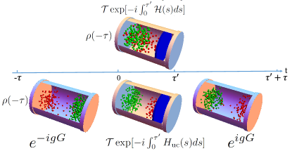
Figure 1: Schematic of a three-stage time evolution picture. The time evolution for an open system with strong SBC during the time interval $[0,\tau^{\prime}]$ is interpreted as the time evolution over $[-\tau,\tau^{\prime}+\tau]$ with the same initial state $\rho(-\tau)$. In this picture, the first and third stages over the time intervals $[-\tau,0]$ and $[\tau^{\prime},\tau+\tau^{\prime}]$ involve heat exchange with a bath under weak SBC without work and the middle stage over the time interval $[0,\tau^{\prime}]$ involves work without heat. Upon our mapping detailed in the main text, both Hamiltonians of the system (red particles) and the bath (green particles) will be corrected by SBC; and the blue piston represents a work protocol.

Mapping between strong and weak SBC—Consider the following composite system-bath Hamiltonian:

$$\mathcal{H}(t)=\mathcal{H}_{\mathrm{s}}(t)+\mathcal{H}_{\mathrm{I}}(t)+\mathcal{H}_{\mathrm{b}}(t),$$ (1)

where $\mathcal{H}_{\mathrm{s}}(t)$ and $\mathcal{H}_{\mathrm{b}}(t)$ are the respective Hamiltonians of the system and the bath, and $\mathcal{H}_{\mathrm{I}}(t)=g\sum\limits_{\mathrm{j}}A_{\mathrm{s}}^{\mathrm{j}}(t)A_{\mathrm{b}}^{\mathrm{j}}(t)$ depicts the SBC, with system operators $A_{\mathrm{s}}^{\mathrm{j}}$ and bath operators $A_{\mathrm{b}}^{\mathrm{j}}$. Here $g$ is the dimensionless SBC strength, with $g\ll 1$ indicating weak coupling and $g\gtrsim 1$ indicating strong coupling.

In treating light-matter interaction [18, 17] or polaronic systems [19], a strong system-bath coupling can be connected with cases of a weak coupling via some unitary transformation. Mimicking but different from this idea, let us now introduce an unitary transformation $e^{igG}$, through which we can connect the original composite system Hamiltonian $\mathcal{H}(t)$ with a system-bath uncoupled Hamiltonian $H_{\mathrm{uc}}$, namely,

$$\mathcal{H}(t)=e^{igG}H_{\mathrm{uc}}(t)e^{-igG},$$ (2)

where the transformation generator $G=\sum\limits_{\mathrm{j}}B_{\mathrm{s}}^{\mathrm{j}}B_{\mathrm{b}}^{\mathrm{j}}$ with $B_{\mathrm{s}}^{\mathrm{j}}$ being system operators and $B_{\mathrm{b}}^{\mathrm{j}}$ being bath operators. The uncoupled Hamiltonian assumes the form of $H_{\mathrm{uc}}(t)=H_{\mathrm{s}}(t)+H_{\mathrm{b}}$, with the transformed system Hamiltonian $H_{\mathrm{s}}(t)$ being time dependent in general, and the transformed bath Hamiltonian $H_{\mathrm{b}}$ being time independent.

For a given $\mathcal{H}(t)$, it appears to be a challenge to transform, via the generator $G$ introduced above, to a system-bath uncoupled Hamiltonian $H_{\mathrm{uc}}(t)$. Since we are more concerned with fundamentals of thermodynamic quantities with strong SBC, we allow ourselves to start with $H_{\mathrm{uc}}$ instead. Nevertheless, because $G$ is arbitrary, in principle the transformation $e^{igG}$ suffices to yield a rather generic $\mathcal{H}_{\mathrm{I}}$ from $H_{\mathrm{uc}}$. Consider then the following explicit example where $H_{\mathrm{uc}}=H_{\mathrm{s}}(t)+H_{\mathrm{b}}$ with $H_{\mathrm{s}}(t)=\lambda_{\mathrm{x}}(t)\sigma_{\mathrm{s}}^{\mathrm{x}}+\lambda_{\mathrm{z}}(t)\sigma_{\mathrm{s}}^{\mathrm{z}}$, $\{\sigma^{i}\}$ the Pauli operators, $\lambda_{\mathrm{x}}(t)$ and $\lambda_{\mathrm{z}}(t)$ two time-dependent paramaters, and $H_{\mathrm{b}}=-\omega_{\mathrm{b}}\sum_{\mathrm{k}}\sigma_{\mathrm{k}}^{\mathrm{z}}-h\sum_{\left\langle\mathrm{k,j}\right\rangle}\sigma_{\mathrm{k}}^{\mathrm{x}}\sigma_{\mathrm{j}}^{\mathrm{x}}$, depicting a spin bath modeled by an Ising model with $N$ spins interacting with the nearest-neighbor sites $\left\langle\mathrm{k,j}\right\rangle$. Planck’s constant is taken as unity throughout. This uncoupled system can be connected with a model where a central spin interacts with an Ising bath [21, 20] by considering $G=\sigma_{\mathrm{s}}^{\mathrm{x}}\sum_{\mathrm{k}}\sigma_{\mathrm{k}}^{\mathrm{x}}$. Using the transformation depicted by Eq. (2) above, one finds $\mathcal{H}_{\mathrm{s}}=H_{\mathrm{s}}(t)=\lambda_{\mathrm{x}}(t)\sigma_{\mathrm{s}}^{\mathrm{x}}+\lambda_{\mathrm{z}}(t)\sigma_{\mathrm{s}}^{\mathrm{z}}$. $\mathcal{H}_{\mathrm{b}}$ differs from the mapped $H_{\mathrm{b}}$, namely, $\mathcal{H}_{\mathrm{b}}=-\omega_{\mathrm{b}}\cos(g)\sum_{\mathrm{k}}\sigma_{\mathrm{k}}^{\mathrm{z}}-h\sum_{\left\langle\mathrm{kj}\right\rangle}\sigma_{\mathrm{k}}^{\mathrm{x}}\sigma_{\mathrm{j}}^{\mathrm{x}}$ [22]. Finally, the original system-bath coupling term $\mathcal{H}_{\mathrm{I}}=-\omega_{\mathrm{b}}\sin(g)\sigma_{\mathrm{s}}^{\mathrm{x}}\sum_{\mathrm{k}}\sigma_{\mathrm{k}}^{\mathrm{y}}+\lambda_{\mathrm{z}}(t)\sigma_{\mathrm{s}}^{\mathrm{z}}[\cos(g\sum_{\mathrm{k}}\sigma_{\mathrm{k}}^{\mathrm{x}})-1]+\lambda_{\mathrm{z}}(t)\sigma_{\mathrm{s}}^{\mathrm{y}}\sin(g\sum_{\mathrm{k}}\sigma_{\mathrm{k}}^{\mathrm{x}})$ [22]. This working example here has thus illustrated that it is feasible to connect an original open quantum system Hamiltonian $\mathcal{H}(t)$ with a system-bath decoupled Hamiltinian $H_{\mathrm{uc}}(t)$. A second example involving a Caldeira-Leggett like model is discussed in Supplementary Materials [22].

The unitary propagator of the original composite system over the time duration $[0,\tau^{\prime}]$ can be formally written as $U_{0\rightarrow\tau^{\prime}}=\mathcal{T}\exp[-i\int_{0}^{\tau^{\prime}}\mathcal{H}(s)ds]$. Thanks to the transformation introduced in Eq. (2), $U_{0\rightarrow\tau^{\prime}}$ can be written as a product of three unitaries: $U_{0\rightarrow\tau^{\prime}}=e^{igG}U_{\mathrm{uc}}e^{-igG}$. In other words, whatever is captured by $U_{0\rightarrow\tau^{\prime}}$ can be digested in terms of three stages, a unitary process $e^{-igG}$ due to our transformation, a unitary propagator $U_{\mathrm{uc}}=\mathcal{T}\exp[-i\int_{0}^{\tau^{\prime}}H_{\mathrm{uc}}(s)ds]$ with system and bath uncoupled, and a third unitary $e^{igG}$ [22] also due to our transformation. This is schematically shown in Fig. 1. A few important remarks are in order. First, by construction, $U_{\mathrm{uc}}$ represents the propagator under $H_{\mathrm{uc}}(t)$. Energy change caused by $U_{\mathrm{uc}}$ is entirely due to work done to the system because there is no system-bath interaction during this step. Secondly, the two unitaries $e^{\pm igG}$ are apparently responsible for energy exchange between system and bath, and hence heat can be extracted from these two processes without arbitrariness while no work protocol is executed (since there are no changes to all the system parameters). Specifically, as shown in Supplementary Materials [22], the two unitary operators $e^{-igG}$ and $e^{igG}$ can be interpreted as the respective outcomes of the time evolution of the composite systems $H_{\mathrm{uc}}(0)$ and $H_{\mathrm{uc}}(\tau^{\prime})$ over a duration defined as $\tau$, evolving under the time-dependent SBC $H_{-}=\frac{g}{\tau}G_{-}$ and $H_{+}=-\frac{g}{\tau}G_{+}$ with $G_{-}=\exp[-iH_{\mathrm{uc}}(0)t]G\exp[iH_{\mathrm{uc}}(0)t]$ and $G_{+}=\exp[-iH_{\mathrm{uc}}(\tau^{\prime})t]G\exp[iH_{\mathrm{uc}}(\tau^{\prime})t]$ [22]. If we now choose $\tau$ to be sufficiently large, then $e^{-igG}$ and $e^{igG}$ represents a slow relaxation process experienced by some quantum open system with weak SBC. This way, time is exploited to uncover a physics-based mapping between strong and weak SBC. Of particular interest is to consider extremely long processes ($\tau\rightarrow+\infty$), such that on the one hand, we can safetly apply our knowledge in the weak SBC regime and on the other hand, one can assume self-relaxation of the composite system $H_{\mathrm{uc}}$ towards its Gibbs state under the actions of $e^{-igG}$ and $e^{igG}$. One may be concerned that turning on the $H{\pm}$ introduced in our picture above can involve work as well. This concern can be lifted because the associated work due to $H_{\pm}$ is inversely proportional to $\tau$ [22]. In the limit of very large $\tau$, such kind of work due to the switching on of SBC vanishes.

Quantum thermodynamics at arbitrary SBC strength—With the above three-stage picture (see Fig. 1), it is now possible to identify basic thermodynamic quantities at arbitrary SBC strength, by use of well-established quantities for weak SBC [5, 24, 25, 26, 6, 7]. As stated above, heat exchange can be calculated based on the propagator associated with the two time intervals $[-\tau,0]$ and $[\tau^{\prime},\tau^{\prime}+\tau]$. There is no conceptual difficulty in doing so because the composite system Hamiltonian is understood to be a static one, namely $H_{\mathrm{uc}}(0)$ or $H_{\mathrm{uc}}(\tau^{\prime})$ during these two stages and hence no work is involved by construction. To arrive at a differential form of heat, we can also take duation $\tau^{\prime}$ to be infinitesimal. We then find that, for an arbitrary coupling strength $g$, heat exchange is given by the following expression [22]:

$$dQ=\mathrm{Tr}_{\mathrm{s}}(H_{\mathrm{s}}~{}d\rho_{\mathrm{s}})+\mathrm{Tr}[\rho~{}d(H_{\mathrm{s}}-\mathcal{H})],$$ (3)

where $\mathrm{Tr}_{\mathrm{s}}(A)$ and $\mathrm{Tr(}A)$ are trace operations over the system and the sytem-bath composite system, respectively. $\rho$ here represents the true initial state of the composite system and $\rho_{\mathrm{s}}$ is the reduced density of the system. The second term in the equation above represents a correction due to SBC, which, as expected, vanishes in cases of vanishingly weak SBC.

Likewise, to identify work done to the system we now turn our attention to the time interval $[0,\tau^{\prime}]$. According to the above three-stage picture again, during the time interval $[0,\tau^{\prime}]$ the system is uncoupled with the bath. Thus, the associated heat transfer is necessarily zero. The work at arbitrary SBC strength is then found to be [22, 29]:

$$dW=\mathrm{Tr}(\rho~{}d\mathcal{H}).$$ (4)

This expression is obtained from a standard calculation of the expectation value of quantum work for an isolated system uncoupled from a bath, fully consistent with the two-time measurement definition of quantum work if the initial state of the work protocol during the time interval $[0,\tau^{\prime}]$ possesses no energy coherence [30].

It is now curious to investigate how the first law of thermodynamics is manifested in cases with strong SBC. Using Eqs. (3) and (4), one finds

$$dE=dW+dQ=d[\mathrm{Tr}_{\mathrm{s}}(H_{\mathrm{s}}\rho_{\mathrm{s}})]$$ (5)

for arbitrary SBC strength. This result is by no means trivial because $H_{\mathrm{s}}$ in Eq. (5) represents the system component of $H_{\mathrm{uc}}$, which is yet to be worked out in order to do explicit calculations. Because one can still imagine a ficticious $H_{\mathrm{s}}$ before it can be found, the first law of thermodynamics under strong SBC is physically intriguing.

Having discussed the first law, next we examine the entropy function $S$ in the presence of strong SBC. To facilitate our investigations let us now specifically consider a quasi-static process such as the composite system stays in its Gibbs state, $\Omega(t)=\exp[-\beta\mathcal{H}(t)]/Z(t)$, where $Z(t)$ is the corresponding partition function and $\beta$ the fixed inverse temperature of a super bath. Likewise, refering to $H_{\mathrm{uc}}=H_{\mathrm{s}}(t)+H_{\mathrm{b}}$, we use $Z_{\mathrm{s}}(t)$ to represent the partition function associated with $H_{\mathrm{s}}(t)$ and $Z_{\mathrm{b}}$ the bath partition function associated with the time-independent bath Hamiltonian $H_{\mathrm{b}}$. The initial state of the composite system is then $\Omega(0)=\exp[-\beta\mathcal{H}(0)]/Z(0).$ We also define $\varpi(t)\equiv\exp[-\beta H_{\mathrm{uc}}(t)]/Z_{\mathrm{uc}}(t)$, with the associated partition function $Z_{\mathrm{uc}}(t)$ for the uncoupled Hamiltonian $H_{\mathrm{uc}}$. Using the expression Eq. (3) for $dQ$, we obtain

$$dS=\beta dQ=-d[\mathrm{Tr}(\Omega_{\mathrm{s}}\ln\varpi_{\mathrm{s}})]-d\ln\frac{Z_{\mathrm{s}}}{Z},$$ (6)

where $\Omega_{\mathrm{s}}=\mathrm{Tr}_{\mathrm{b}}(\Omega)$ and $\varpi_{\mathrm{s}}=\mathrm{Tr}_{\mathrm{b}}(\varpi)$ are the reduced state of the system after tracing $\Omega$ and $\varpi$ over the bath, respectively. Further using $Z(t)=\mathrm{Tr}[e^{-\beta\mathcal{H}(t)}]=\mathrm{Tr}[e^{igG}e^{-\beta H_{\mathrm{uc}}(t)}e^{-igG}]=\mathrm{Tr}[e^{-\beta H_{\mathrm{uc}}(t)}]=Z_{\mathrm{uc}}(t)=Z_{\mathrm{s}}(t)Z_{\mathrm{b}}$, the relation $\frac{Z(t)}{Z_{\mathrm{s}}(t)}=Z_{\mathrm{b}}$ becomes evident and so the term $d\ln\frac{Z_{\mathrm{s}}}{Z}$ in Eq. (6) vanishes, yielding

$$dS=-d\mathrm{Tr}(\Omega_{\mathrm{s}}\ln\varpi_{\mathrm{s}}).$$ (7)

This expression for $dS$ can be further rewritten as

$$dS=dS_{v}(\Omega_{\mathrm{s}})+dD(\left.\Omega_{\mathrm{s}}\right|\varpi_{\mathrm{s}}),$$ (8)

where the von Neumann entropy $S_{v}(\Omega_{\mathrm{s}})=-\mathrm{Tr}_{\mathrm{s}}(\Omega_{\mathrm{s}}\ln\Omega_{\mathrm{s}})$, and the relative entropy is $D(\left.\Omega_{\mathrm{s}}\right|\varpi_{\mathrm{s}})=\mathrm{Tr}_{\mathrm{s}}(\Omega_{\mathrm{s}}\ln\Omega_{\mathrm{s}})-\mathrm{Tr}_{\mathrm{s}}(\Omega_{\mathrm{s}}\ln\varpi_{\mathrm{s}})$. We shall return to this useful definition later. For general nonequilbrium situations, the change in the thermal entropy cannot be calculated from the time-evolving non-equilibrium state. Nevertherless, one still wishes to define a change in some information entropy measure. One possible quantity to measure information entropy change for nonequilibrium cases with arbitrary SBC strength can be $\Delta S=\Delta S_{v}(\rho_{\mathrm{s}})+\Delta D(\left.\Omega_{\mathrm{s}}\right|\varpi_{\mathrm{s}})$, which differs from the quasi-static situations by replacing the Gibbs state in a quasi-static process with the actual reduced state of the system $\rho_{\mathrm{s}}$ in a general process.

Fluctuation theorems with arbitrary SBC strength– Our treatment outlined above makes it straightforward to investigate the work fluctuation theorems since the work done can be calculated entirely by the middle step of the above outlined three-stage time evolution. That is, work can be calculated during the $[0,\tau^{\prime}]$ interval only, with the mapped system $H_{\mathrm{s}}(t)$ entirely decoupled from any bath. As such, work fluctuations of the orginal problem become that of the transformed system Hamiltonian $H_{\mathrm{s}}(t)$, of which the time dependence does indicate a possible work protocol. To proceed with explicit calculations, we assume that the initial state of the original problem is still the Gibbs state $\Omega(0)$. During the period of $[-\tau,0]$ that could be arbitrarily long, $\Omega(0)$ evolves to $\varpi(0)$ at the end of the first stage or at the beginning of the middle stage. The so-called characteristic function of work can then be calculated from $\Theta_{0\rightarrow\tau^{\prime}}(u)=\int dw~{}e^{iuw}p_{0\rightarrow\tau^{\prime}}(w)$, where $p_{0\rightarrow t}(w)$ is the probability density of work value $w$ in the middle stage. Adopting the standard treatment in the literature [24], we can express $\Theta_{0\rightarrow\tau^{\prime}}(u)$ in terms of the propagator $U_{\mathrm{uc}}$ associated with $[0,\tau^{\prime}]$. That is, $\Theta_{0\rightarrow\tau^{\prime}}(u)=\mathrm{Tr}\left[U_{\mathrm{uc}}^{\dagger}e^{iuH_{\mathrm{uc}}(\tau^{\prime})}U_{\mathrm{uc}}e^{-(\beta+iu)H_{\mathrm{uc}}(0)}\right]/{Z_{\mathrm{uc}}(0)}$. Further using $U_{0\rightarrow\tau^{\prime}}=e^{igG}U_{\mathrm{uc}}e^{-igG}$, $\mathcal{H}(t)=e^{igG}H_{\mathrm{uc}}(t)e^{-igG}$, and $Z(t)=Z_{\mathrm{uc}}(t)$, one directly obtains

$$\Theta_{0\rightarrow\tau^{\prime}}(u)=\mathrm{Tr}\left[U_{0\rightarrow\tau^{\prime}}^{\dagger}e^{iu\mathcal{{H}(\tau^{\prime})}}U_{0\rightarrow\tau^{\prime}}e^{-(\beta+iu)\mathcal{H}(0)}\right]/{Z(0)}.$$ (9)

Equation (9) suggests that work fluctuation theorems are extendable to cases with arbitrary SBC strength. In particular, given that $U_{0\rightarrow\tau^{\prime}}=U_{\tau^{\prime}\rightarrow 0}^{\dagger}$, one immediately derives from Eq. (9) via an inverse Fourier transformation the following Tasaki-Crooks quantum fluctuation relation:

$$\frac{p_{0\rightarrow\tau^{\prime}}(w)}{p_{\tau^{\prime}\rightarrow 0}(-w)}=\frac{Z(\tau^{\prime})}{Z(0)}e^{\beta w}.$$ (10)

This quantum fluctuation theorem much resembles to that for weak SBC. It should be highlighted that the partition function in the above expression is that of the composite total system, an intriguing result echoing with a previous elegant result [8]. Furthermore, as already suggested in our use of $Z_{\mathrm{uc}}(t)=Z(t)$ in obtaining Eq. (10) above, the above Tasaki-Crooks quantum fluctuation can be also expressed as

$$\frac{p_{0\rightarrow\tau^{\prime}}(w)}{p_{\tau^{\prime}\rightarrow 0}(-w)}=\frac{Z_{\mathrm{s}}(\tau^{\prime})}{Z_{\mathrm{s}}(0)}e^{\beta w},$$ (11)

where $Z_{\mathrm{s}}(t)$ is the system partition function of $H_{\mathrm{s}}(t)$, the system part of the mapped uncoupled Hamiltonian $H_{\mathrm{uc}}(t)$.

One can further extend the celebrated Jarzynski equality to cases with arbitrary SBC strength. Indeed, one can make use of Eq. (11) by integrating $e^{-\beta w}p_{0\rightarrow\tau^{\prime}}(w)$ over all possible work values $w$, arriving at

$$\langle e^{-\beta w}\rangle=\frac{Z_{\mathrm{s}}(\tau^{\prime})}{Z_{\mathrm{s}}(0)}\equiv e^{-\Delta F}.$$ (12)

In the expression above, we have also defined the free energy $F$ associated with $H_{\mathrm{s}}$ when it is in thermal equibrium at temperature $T$, namely, $F\equiv-T\ln Z_{\mathrm{s}}$ and $\Delta F=-T[\ln Z_{\mathrm{s}}(\tau^{\prime})-\ln Z_{\mathrm{s}}(0)]$. Interestingly, with this definition and our early defined entropy $\Delta S$, one finds $\Delta F=\Delta E-T\Delta S$ [22], which is again analgous to the corresponding thermodynamic relation for a constant-temperature process under weak SBC.

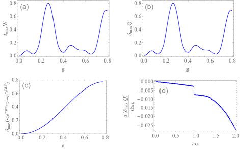
Figure 2: Difference between the strongly and weakly coupled quantum thermodynamics. (a), (b) and (c), respectively, show $\delta_{\max}W$, $\delta_{\max}Q$ and $\delta_{\max}(\left\langle e^{-\beta w_{\mathrm{w}}}\right\rangle-e^{-\beta\Delta F})$ as a function of coupling strength $g$ with $\omega_{\mathrm{b}}=1$; (d) show $\frac{d(\delta_{\max}Q)}{d\omega_{\mathrm{b}}}$ as a function of $\omega_{\mathrm{b}}$ with coupling strength $g=0.1$. The initial state is the Gibbs state $\Omega$ with the invere temperature $\beta=1$. The other parameters are chosen as, $h=1$, $\lambda_{\mathrm{x}}(0)=1$, $\lambda_{\mathrm{z}}(0)=2.5$, ramping rate $\alpha_{\mathrm{x}}=1$, $\alpha_{\mathrm{z}}=-0.6$, number of bath spins $N=6$ and duration time $\tau^{\prime}=2$.

Numerical Results—We further use the central spin model presented above as an example. This model is much similar to that in [31] to study quantum criticality vs the Loschmidt echo if the parameter $\lambda_{\mathrm{z}}$ is zero. The system-bath coupling term $\mathcal{H}_{\mathrm{I}}$ is equivalent to the Heisenberg XY interaction if the parameter $g$ is small [32]. In our simulation, the system is driven through following protocol, i.e., $\lambda_{\mathrm{z}}(t)=\lambda_{\mathrm{z}}(0)(1+\alpha_{z}t)$ and $\lambda_{\mathrm{x}}(t)=\lambda_{\mathrm{x}}(0)(1+\alpha_{x}t)$ with the ramping rate $\alpha_{z}$ and $\alpha_{x}$. The uncoupled bath upon the mapping is a simple one-dimensional Ising model.

We calculate numerically the absolute differences in work and heat between what we defined with our approach and a direct but incorrect application of the weak SBC expression, during the time interval $[0,t]\subset[0,\tau^{\prime}]$. We denote such differences by $\delta W$ and $\delta Q$ [33]. We then record the maximal differences during $[0,\tau^{\prime}]$ to measure the effect of SBC, denoted as $\delta_{\max}W$ and $\delta_{\max}Q$, respectively. Figure 2(a) and 2(b) depicts $\delta_{\max}W$ and $\delta_{\max}Q$ as a function of the SBC strength $g$. It is seen that as the SBC strength $g$ increases, the basic quantities such as work and heat are more affected accordingly.

The impact of an increasing SBC strength on work values has a profound implication for our understanding of the the Jarzynski equality. As a known result, the second law $\left\langle W\right\rangle\geq\Delta F$ can be recovered from the Jarzynski equality by the inequality $\left\langle e^{y}\right\rangle\geq e^{\left\langle y\right\rangle}$, provided that the involved work values and free energy quantities are physically valid. It is thus interesting to ask what happens if one naively calculate the weak-SBC work from $w_{\mathrm{w}}=\int\limits_{0}^{\tau^{\prime}}\mathrm{Tr}_{\mathrm{s}}~{}(\rho_{\mathrm{s}}\ dH_{\mathrm{s}})$ (which is valid only for weak SBC) and then compare $\left\langle e^{-\beta w_{\mathrm{w}}}\right\rangle$ and $e^{-\beta\Delta F}$ through $\delta_{\max}(\left\langle e^{-\beta w_{\mathrm{w}}}\right\rangle-e^{-\beta\Delta F})$, as shown in Fig. 2(c). Clearly, we see that ensemble average of $e^{-\beta w_{\mathrm{w}}}$ does not yield a fixed quantity determined by a free energy difference. If this were true, one might even deduce the possibility of a violation of the second law. This serious situation is rectified if we replace the wrongly calculated $w_{\mathrm{w}}$ by the work $w$ we derived above, resulting in a Jayzynski equality again, independent of the SBC strength.

It is also intriguing to note that the uncoupled bath $H_{\mathrm{b}}$ accommodate a quantum phase transition at the critical point $h=\omega_{\mathrm{b}}$. This phase transition is also detected by the sudden jump in the rate of change of the quantity $\delta_{\max}Q$ with respect to $\omega_{\mathrm{b}}$ (i.e., $d(\delta_{\max}Q)/d\omega_{\mathrm{b}}$), as shown in Fig. 2(d).

Conclusion.—We have theoretically presented an innovative approach to the treatment of open quantum systems with strong SBC, by mapping such systems to cases without system-bath coupling at all. Our approach makes it possible, at least for one wide class of problems where the said mapping can be assumed, to define and calculate thermodynamic quantities with arbitrary SBC, including work and heat. The required mapping might not be easy to find, but even without finding it explicitly, our approach is of theoretical interest because it indicates the existence of well-defined thermodynamic quantities and allows for extensions of quantum fluctuation theorems to arbitrary SBC strength. Our theoretical results are further illustrated with a working example, where the impact of strong SBC can be quantitatively studied.

Acknowledgments.–Valuable discussions with Mang Feng, Jian-Hui Wang and Bei-Lok Hu are gratefully acknowledged. Research by J.G. is supported by the National Research Foundation, Singapore and A*STAR under its CQT Bridging Grant. This work was also funded by National Key R&D Program of China under grants No. 2021YFA1400900, 2021YFA0718300, 2021YFA1400243, NSFC under grants Nos. 11965012, 61835013, 12234012, Space Application System of China Manned Space Program and Yunan Province’s Hi-tech Talents Recruitment Plan No. YNWR-QNBJ-2019-245.

Supplementary Material

I Details of the three-stage picture of the time evolution of quantum open systems with strong system-bath coupling

Based on Eq. (2) in the maintext, the time evolution operator of the original system $\mathcal{H}$ can be written as

$$U_{0\rightarrow\tau^{\prime}}=e^{igG}U_{\mathrm{uc}}e^{-igG}.$$ (S1)

Next we can view the unitary operators $e^{-igG}$ and $e^{+igG}$ as two respective unitary operators associated with Hamiltonians $\pm G$ in some interaction representation respectively associated with $H_{\mathrm{uc}}(0)$ and $H_{\mathrm{uc}}(\tau^{\prime})$. With this understanding, we can proceed to rewrite the above expression into the following product:

$$U_{0\rightarrow\tau^{\prime}}=U_{\mathrm{w\tau}^{\prime}}U_{\mathrm{uc}}U_{\mathrm{w0}},$$ (S2)

where

$$U_{\mathrm{w0}} = \exp[iH_{\mathrm{uc}}(0)\tau]\mathcal{T}\left[\exp\{-i\int_{0}^{\tau}[H_{\mathrm{uc}}(0)+\frac{g}{\tau}G_{-}(s)]ds\}\right]$$ (S3)

$$U_{\mathrm{w\tau}^{\prime}} = \exp[iH_{\mathrm{uc}}(\tau^{\prime})\tau]\mathcal{T}\left[\exp\{-i\int_{0}^{\tau}[H_{\mathrm{uc}}(\tau^{\prime})-\frac{g}{\tau}G_{+}(s)]ds\}\right].$$ (S4)

with

$$G_{-}(t) = \exp[-iH_{\mathrm{uc}}(0)t]G\exp[iH_{\mathrm{uc}}(0)t]$$ (S5)

$$G_{+}(t) = \exp[-iH_{\mathrm{uc}}(\tau^{\prime})t]G\exp[iH_{\mathrm{uc}}(\tau^{\prime})t].$$ (S6)

The above relations become more obvious if one considers the following equalities

$$\tilde{U}_{\mathrm{w0}}(t) = \mathcal{T}\left[\exp\{-i\int_{0}^{t}[H_{\mathrm{uc}}(0)+\frac{g}{\tau}G_{-}(s)]ds\}\right];$$ (S7)

$$= \exp[-iH_{\mathrm{uc}}(0)t]\exp[-i\frac{g}{\tau}Gt]$$

$$\tilde{U}_{\mathrm{w\tau}^{\prime}}(t) = \mathcal{T}\left[\exp\{-i\int_{0}^{t}[H_{\mathrm{uc}}(\tau^{\prime})+\frac{g}{\tau}G_{+}(s)]ds\}\right]$$ (S8)

$$= \exp[-i[H_{\mathrm{uc}}(\tau^{\prime})t]\exp[i\frac{g}{\tau}Gt],$$

both of which can be directly proven by differentiating $\tilde{U}_{\mathrm{w0}}(t)$ and $\tilde{U}_{\mathrm{w\tau}^{\prime}}(t)$ defined above with respect to variable $t$.

It is now interesting to comment on the three exponentials in Eq. (S2). First of all, the evolution operators $\exp[iH_{\mathrm{uc}}(0)\tau]$ and $\exp[iH_{\mathrm{uc}}(\tau^{\prime})\tau]$ as prefactors of $U_{\mathrm{w0}}$ and $U_{\mathrm{w\tau^{\prime}}}$ shown in Eq. (S3) and Eq. (S4) are referring to evolution operators of certain fixed system-bath decoupled Hamiltonians: hence neither work or heat will be involved. Seondly, as the chosen $\tau$ becomes very long, the time-dependent Hamiltonians $H_{\mathrm{uc}}(0)+\frac{g}{\tau}G_{-}(t)$ or $H_{\mathrm{uc}}(\tau^{\prime})-\frac{g}{\tau}G_{+}(t)$ used in the expressions for Eq. (S3) and Eq. (S4) have vanishingly small (though time-dependent) system-bath coupling: hence only heat will be involved in such processes. That is, the work needed to turn on the time-dependent Hamiltonians are $W_{\pm}=\mp\int\mathrm{Tr}(\frac{g}{\tau}\rho\ dG_{\pm})=\mp\frac{g}{\tau}\Delta\mathrm{Tr}(\rho G_{\pm})$, which will be vanishing in the limit $\tau\rightarrow\infty$. This completes our three-stage time evolution picture: $U_{\mathrm{w\tau}^{\prime}}$ and $U_{\mathrm{w0}}$ will incur heat exchange whereas $U_{\mathrm{uc}}$ will be responsible for work. This way, we have identified one clear-cut route towards explicit calculations of heat and work without any ambiguity.

II Models

To elaborate on the mapping between strong and weak SBC in more detail, we first consider a central spin-$\frac{1}{2}$ interacting with a spin bath, an example mainly used by the main text. According to the main text, the system-bath uncoupled Hamiltonian upon a desired mapping is

$$H_{\mathrm{uc}}=H_{\mathrm{s}}(t)+H_{\mathrm{b}},$$ (S9)

where the central spin Hamiltonian is $H_{\mathrm{s}}(t)=\lambda_{\mathrm{x}}(t)\sigma_{\mathrm{s}}^{\mathrm{x}}+\lambda_{\mathrm{z}}(t)\sigma_{\mathrm{s}}^{\mathrm{z}}$, $\{\sigma^{\mathrm{i}}\}$ are the Pauli operators, $\lambda_{\mathrm{x}}(t)$ and $\lambda_{\mathrm{z}}(t)$ are two time-dependent paramaters, and the spin bath Hamiltonian $H_{\mathrm{b}}=-\omega_{\mathrm{b}}\sum_{\mathrm{k}}\sigma_{\mathrm{k}}^{\mathrm{z}}-h\sum_{\left\langle\mathrm{k,j}\right\rangle}\sigma_{\mathrm{k}}^{\mathrm{x}}\sigma_{\mathrm{j}}^{\mathrm{x}}$ is that of an Ising chain.

So what kind of original composite system Hamiltonian $\mathcal{H}(t)$ can be mapped to the $H_{\mathrm{uc}}$ specified in Eq. (S9) above? To that end we first show how to derive the following relation:

$$\exp(ig\Sigma^{\mathrm{x}}J^{\mathrm{x}})J^{\mathrm{z}}\exp(-ig\Sigma^{\mathrm{x}}J^{\mathrm{x}})=J^{\mathrm{z}}\cos(g\Sigma^{\mathrm{x}})+J^{\mathrm{y}}\sin(g\Sigma^{\mathrm{x}}),$$ (S10)

where $\{\Sigma^{\mathrm{x}}\}$ and $\{J^{\mathrm{z}}\}$, respectively, are the angular momentum operators for two different spin systems along directions $x$, $z$ etc. To otain this relation, we first use the Baker-Hausdorff lemma such that the left-hand side of the above equation can be written as

$$\exp(ig\Sigma^{\mathrm{x}}J^{\mathrm{x}})J^{\mathrm{z}}\exp(-ig\Sigma^{\mathrm{x}}J^{\mathrm{x}}) = J^{\mathrm{z}}+[ig\Sigma^{\mathrm{x}}J^{\mathrm{x}},J^{\mathrm{z}}]+\frac{1}{2!}[ig\Sigma^{\mathrm{x}}J^{\mathrm{x}},[ig\Sigma^{\mathrm{x}}J^{\mathrm{x}},J^{\mathrm{z}}]]$$ (S11)

$$+\frac{1}{3!}[ig\Sigma^{\mathrm{x}}J^{\mathrm{x}},[ig\Sigma^{\mathrm{x}}J^{\mathrm{x}},[ig\Sigma^{\mathrm{x}}J^{\mathrm{x}},J^{\mathrm{z}}]]]+\cdots.$$

With the commutators of angular momentum, it can be simplified to

$$\exp(ig\Sigma^{\mathrm{x}}J^{\mathrm{x}})J^{\mathrm{z}}\exp(-ig\Sigma^{\mathrm{x}}J^{\mathrm{x}})=J^{\mathrm{z}}+g\Sigma^{\mathrm{x}}J^{\mathrm{y}}-\frac{1}{2!}(g\Sigma^{\mathrm{x}})^{2}J^{\mathrm{z}}-\frac{1}{3!}(g\Sigma^{\mathrm{x}})^{3}J^{\mathrm{y}}+\cdots$$

$$=J^{\mathrm{z}}\cos(g\Sigma^{\mathrm{x}})+J^{\mathrm{y}}\sin(g\Sigma^{\mathrm{x}}),$$ (S12)

which is just the relation we hope to derive.

Applying the relation of Eq. (S10) to the expressions $\exp(igG)\sigma_{\mathrm{s}}^{\mathrm{z}}\exp(-igG)$ and $\exp(igG)\sigma_{\mathrm{k}}^{\mathrm{z}}\exp(-igG)$ with $G=\sigma_{\mathrm{s}}^{\mathrm{x}}\sum_{\mathrm{k}}\sigma_{\mathrm{k}}^{\mathrm{x}}$, we obtain

$$\mathcal{H}(t) = \lambda_{\mathrm{x}}(t)\sigma_{\mathrm{s}}^{\mathrm{x}}-\cos(g)\omega_{\mathrm{b}}\sum_{\mathrm{k}}\sigma_{\mathrm{k}}^{\mathrm{z}}-h\sum_{\left\langle\mathrm{k,j}\right\rangle}\sigma_{\mathrm{k}}^{\mathrm{x}}\sigma_{\mathrm{j}}^{\mathrm{x}}$$

$$+\lambda_{\mathrm{z}}(t)[\sigma_{\mathrm{s}}^{\mathrm{z}}\cos(g\sum_{\mathrm{k}}\sigma_{\mathrm{k}}^{\mathrm{x}})+\sigma_{\mathrm{s}}^{\mathrm{y}}\sin(g\sum_{\mathrm{k}}\sigma_{\mathrm{k}}^{\mathrm{x}})]-\omega_{\mathrm{b}}\sin(g)\sigma_{\mathrm{s}}^{\mathrm{x}}\sum_{\mathrm{k}}\sigma_{\mathrm{k}}^{\mathrm{y}},$$

which can be rewritten as $\mathcal{H}(t)=\mathcal{H}_{\mathrm{s}}+\mathcal{H}_{\mathrm{I}}+\mathcal{H}_{\mathrm{b}}$, with

$$\mathcal{H}_{\mathrm{s}} = \lambda_{\mathrm{x}}(t)\sigma_{\mathrm{s}}^{\mathrm{x}}+\lambda_{\mathrm{z}}(t)\sigma_{\mathrm{s}}^{\mathrm{z}},$$

$$\mathcal{H}_{\mathrm{b}} = -\cos(g)\omega_{\mathrm{b}}\sum_{\mathrm{k}}\sigma_{\mathrm{k}}^{\mathrm{z}}-h\sum_{\left\langle\mathrm{k,j}\right\rangle}\sigma_{\mathrm{k}}^{\mathrm{x}}\sigma_{\mathrm{j}}^{\mathrm{x}},$$

$$\mathcal{H}_{\mathrm{I}} = -\omega_{\mathrm{b}}\sin(g)\sigma_{\mathrm{s}}^{\mathrm{x}}\sum_{\mathrm{k}}\sigma_{\mathrm{k}}^{\mathrm{y}}+\lambda_{\mathrm{z}}(t)\sigma_{\mathrm{s}}^{\mathrm{z}}[\cos(g\sum_{\mathrm{k}}\sigma_{\mathrm{k}}^{\mathrm{x}})-1]+\lambda_{\mathrm{z}}(t)\sigma_{\mathrm{s}}^{\mathrm{y}}\sin(g\sum_{\mathrm{k}}\sigma_{\mathrm{k}}^{\mathrm{x}}).$$ (S13)

If the coupling strength $g$ is sufficiently small, one may Taylor expand the sine and cosine functions in the expression for $\mathcal{H}_{\mathrm{I}}$ above, reducing it to $\mathcal{H}_{\mathrm{I}}=-g\omega_{\mathrm{b}}\sigma_{\mathrm{s}}^{\mathrm{x}}\sum_{\mathrm{k}}\sigma_{\mathrm{k}}^{\mathrm{y}}+g\lambda_{\mathrm{z}}(t)\sigma_{\mathrm{s}}^{\mathrm{y}}\sum_{\mathrm{k}}\sigma_{\mathrm{k}}^{\mathrm{x}}$. Summarizing our explicit calculations above as an example, the key message is that an open quantum system with $\mathcal{H}_{\mathrm{s}}$, $\mathcal{H}_{\mathrm{b}}$, and $\mathcal{H}_{\mathrm{I}}$ as above can indeed be mapped onto a system-bath decoupled system $H_{\mathrm{uc}}$ through the generator $G=\sigma_{\mathrm{s}}^{\mathrm{x}}\sum_{\mathrm{k}}\sigma_{\mathrm{k}}^{\mathrm{x}}$. Indeed, with this “reversed engineering” approach, it is clear that a wide variety of mapping between an original quantum open system and $H_{\mathrm{uc}}$ can be generated by choosing different $G$ as the mapping generators. The existence of this kind of mapping within such a class of problems indicates that we can push thermodynamics concepts to the strong SBC regime without any conceptual difficulty.

As a second example we now discuss a Caldeira-Leggett like model that can be mapped onto a system-bath decoupled model $H_{\mathrm{uc}}=H_{b}+H_{\mathrm{s}}(t)$, with $H_{b}=\sum_{k}\omega_{k}a_{k}^{\dagger}a_{k}$, and $H_{\mathrm{s}}(t)=\frac{p_{\mathrm{s}}^{2}}{2m}+\frac{1}{2}\lambda_{t}{x_{\mathrm{s}}}^{2}$, where $\lambda_{t}$ a time-depenndent parameter due to the change of the trapping frequency in a work protocol. For future reference we also define $q_{k}=(a_{k}^{\dagger}+a_{k})$ and $\pi_{k}=i(a_{k}^{\dagger}-a_{k})$. Consider then again the transformation $\mathcal{H}(t)=e^{igG}H_{\mathrm{uc}}(t)e^{-igG}$, now with $G=p_{\mathrm{s}}\sum g_{k}(a_{k}^{\dagger}+a_{k})$. Through the property of displacement operator $D(-\alpha)aD(\alpha)=a+\alpha$ with $D(\alpha)=\exp(\alpha a^{\dagger}-\alpha^{\ast}a)$, we obtain

$$e^{igG}(\sum\omega_{k}a_{k}^{\dagger}a_{k})e^{-igG}=\sum\omega_{k}(a_{k}^{\dagger}-igg_{k}p_{\mathrm{s}})(a_{k}+igg_{k}p_{\mathrm{s}}),$$ (S14)

and

$$e^{igG}[\frac{1}{2m}p_{\mathrm{s}}^{2}+V(\lambda_{t},x_{\mathrm{s}})]e^{-igG}=\frac{1}{2m}p_{\mathrm{s}}^{2}+V(\lambda_{t},x_{\mathrm{s}}-\sqrt{2}g\sum g_{k}q_{k}),$$ (S15)

where $V(\lambda_{t},x)=\frac{1}{2}\lambda_{t}x^{2}$ is the potential function. Combining these two equations, the original system Hamiltonian $\mathcal{H}_{s}$ of a Caldeira-Leggett like model is found to be

$$\mathcal{H}_{\mathrm{s}}=\frac{1}{2M_{\mathrm{s}}}p_{\mathrm{s}}^{2}+V(\lambda_{t},x_{\mathrm{s}}),$$ (S16)

where $M_{\mathrm{s}}=m/(1+$ $2mg^{2}\sum_{\mathrm{k}}\omega_{\mathrm{k}}g_{\mathrm{k}}^{2})$ is the renormalized mass. The orginal $\mathcal{H}_{\mathrm{b}}$ before the mapping also differs from the $H_{\mathrm{b}}$ after the mapping, namely,

$$\mathcal{H}_{\mathrm{b}}=\sum_{\mathrm{k}}\omega_{\mathrm{k}}a_{\mathrm{k}}^{\dagger}a_{\mathrm{k}}+\frac{1}{2}\lambda_{\mathrm{t}}(g\sum_{\mathrm{k}}g_{\mathrm{k}}q_{\mathrm{k}})^{2}.$$ (S17)

Finally, the original system-bath coupling term before the mapping:

$$\mathcal{H}_{\mathrm{I}}=g\lambda_{\mathrm{t}}x_{\mathrm{s}}\sum_{\mathrm{k}}g_{\mathrm{k}}q_{\mathrm{k}}+gp_{\mathrm{s}}\sum_{\mathrm{k}}g_{\mathrm{k}}\pi_{\mathrm{k}},$$ (S18)

where the first term is the standard interaction Hamiltonian adopted in the Caldeira-Leggett model, with $gg_{\mathrm{k}}$ depicting the coupling strength between the system and the $\mathrm{k}$th harmonic oscillator. This second working example further illustrates that it is feasible to connect an original open quantum system Hamiltonian $\mathcal{H}(t)$ with a system-bath decoupled Hamiltonian $H_{\mathrm{uc}}(t)$ through a mapping. The existence of a mapping in such class of problems makes it possible to work on quantum thermodynamic quantities rigorously and identify the underlying fluctuation theorems, as shown in the main text and later sections here.

To complement the simulation results presented in the main text using the spin model, in this supplementary material, we shall also use the above Caldeira-Leggett like model to further illustrate our results. Specifically, we consider a simple physical situation motivated by the specific physical context of sympathetic cooling of atomic gases [1]. Consider then Cs-Li atoms [2] [likewise, K-Rb atoms studied in Ref. [3]] trapped in an optical dipole trap [2] approximated by harmonic potentials [4]. In our example, we take a lithium atom as system and a cesium atom as the bath. To further simplify the problem, we only consider one of the radial oscillations. The composite system is then reduced to one harmonic oscillator interacting with a single free oscillator as the bath, with $H_{\mathrm{b}}=\omega_{\mathrm{Cs}}^{\mathrm{r}}a^{\dagger}a$. The system Hamiltonian is taken as $H_{\mathrm{s}}(t)=\frac{p_{\mathrm{s}}^{2}}{2m}+\frac{1}{2}m\omega_{\mathrm{s}}^{2}(t)x^{2}$ with $\omega_{\mathrm{s}}(t)=\omega_{\mathrm{Li}}^{\mathrm{r}}(1+\alpha t)$ and the trapping-frequency ramping rate $\alpha$. According to our discussions above, the expression of $\mathcal{H}(t)$ mapped to such $H_{\mathrm{uc}}=H_{\mathrm{s}}(t)+H_{\mathrm{b}}$ can be easily found if we use $G=p_{\mathrm{s}}g(a^{\dagger}+a)$.

III Quantum thermodynamics with weak system-bath coupling

To appreciate the treatment we put forward in the main text to handle open quantum systems with strong SBC, it is necessary to recap some known results of quantum thermodynamics under the assumption of weak SBC. To consider cases with vanishingly small SBC, it is convinient to simply use $H_{\mathrm{s}}$ and $H_{\mathrm{b}}$ to denote the system and bath Hamiltonians respectively, the notation deliberately chosen to be the same as what is used in the main text when considering the uncoupled Hamiltonian in the three-stage time evolution picture. We also use $H_{\mathrm{uc}}=H_{\mathrm{s}}+H_{\mathrm{b}}$ to represent the whole system-bath Hamiltonian, upon neglecting their coupling. The system and bath as a whole isolated system will be thermalized to the following equilibrium state $\Omega_{\mathrm{uc}}=\frac{1}{Z_{\mathrm{uc}}}\exp(-\beta H_{\mathrm{uc}})$, where $Z_{\mathrm{u}c}=\mathrm{Tr}[\exp(-\beta{H}_{\mathrm{uc}})]$ is the partition function, $\beta=1/T$ is the inverse temperature of a super bath, and the Boltzmann constant is set to $k_{B}=1$. Since we have assumed vanishingly small weak SBC, this equilibrium state results in the system’s equilibrium reduced state, $\varpi_{\mathrm{s}}=\exp(-\beta H_{{s}})/Z_{\mathrm{s}}$, where $Z_{\mathrm{s}}$ is the associated partition function of $H_{\mathrm{s}}$.

Under weak SBC, the basic quantum thermodynamic quantities can be defined as follows. First, one may define work as [5]

$$dW_{\mathrm{w}}=\mathrm{Tr}_{\mathrm{s}}(\rho_{\mathrm{s}}\ dH_{\mathrm{s}}),$$ (S19)

where $\rho_{\mathrm{s}}=\mathrm{Tr}_{\mathrm{b}}(\rho)$ and $\rho$ are the density matrices of the system and the overall system-bath as a whole system, respectively. Here and later we use the subscript or supercript “w” to highlight that we are working with the conventional work and heat quantities under weak SBC. This definition of work has been applied to both the equilibrium thermodynamics and non-equilibrium processes because it is fully consistent with the well-known two-time energy measurement operation definition if the initial state does not have coherence between energy eigenstates.

On the other hand, the change of the total internal energy of the system can be captured by

$$dE=d\mathrm{Tr}_{\mathrm{s}}(\rho_{\mathrm{s}}H_{\mathrm{s}}).$$ (S20)

Consider now a process where $dW_{\mathrm{w}}=0$, then all the internal energy change should be due to heat exchange. That is, $dQ_{\mathrm{w}}=dE$ with $\mathrm{Tr}_{\mathrm{s}}(\rho_{\mathrm{s}}\ dH_{\mathrm{s}})=0$. This indicates that

$$dQ_{\mathrm{w}}=\mathrm{Tr}_{\mathrm{s}}(H_{\mathrm{s}}\ d\rho_{\mathrm{s}}).$$ (S21)

One can further proceed to define the free energy and the thermodynamic entropy, respectively:

$$F_{\mathrm{w}} = -T\ln Z_{\mathrm{s}},$$

$$S_{\mathrm{w}} = S_{\mathrm{v}}(\varpi_{\mathrm{s}}),$$ (S22)

where $S_{\mathrm{v}}(\rho_{\mathrm{s}})=-\mathrm{Tr}_{\mathrm{s}}(\rho_{\mathrm{s}}\ln\rho_{\mathrm{s}})$ is the von Neumann entropy of the equilibrium state $\rho_{\mathrm{s}}$. That is, for equilbirum situations with weak SBC, the thermodynamics entropy equals to the von Neumann entropy of the equilibrium state $\varpi_{\mathrm{s}}$. One can confirm this result by further using the relation $dS_{\mathrm{w}}=\beta dQ_{\mathrm{w}}$. Using these treatments, other thermodynamics relations such as $F_{\mathrm{w}}=E-TS_{\mathrm{w}}$ and $S_{\mathrm{w}}=-[\partial F_{\mathrm{w}}/\partial T]_{V}$ can be all recovered.

For later discussions, it is also necessary to first discuss known quantum fluctuation theorems with weak SBC. To that end let us focus on the seminal quantum Tasaki-Crooks fluctuation theorem [6]. We assume that the system is isolated from the bath when work is done during the time interval of $[t_{0},t]$ and that work done can be measured through the well-known two-time energy measurement protocol. The fluctuation of work can be fully characterized by the work probability density $p_{t_{0}\rightarrow t}^{\mathrm{w}}(w)$. The so-called characteristic function of work can be defined as the Fourier transform of the work probability density $p_{t_{0}\rightarrow t}^{\mathrm{w}}(w)$, namely,

$$\Theta_{t_{0}\rightarrow t}^{\mathrm{w}}(u)=\int dwe^{iuw}p_{t_{0}\rightarrow t}^{\mathrm{w}}(w).$$ (S23)

As explicitly shown in [7], this characteristic function is connected with the system’s time evolution operators through

$$\Theta_{t_{0}\rightarrow t}^{\mathrm{w}}(u)=Z_{\mathrm{s}}(t_{0})^{-1}\mathrm{Tr}_{\mathrm{s}}[U_{t_{0}\rightarrow t}^{\mathrm{s}\dagger}e^{iuH_{\mathrm{s}}(t)}U_{t_{0}\rightarrow t}^{\mathrm{s}}e^{-iuH_{\mathrm{s}}(t_{0})}e^{-\beta H_{\mathrm{s}}(t_{0})}],$$ (S24)

where the partition function of the system is $Z_{\mathrm{s}}(t_{0})=\mathrm{Tr}_{\mathrm{s}}[e^{-\beta H_{\mathrm{s}}(t_{0})}]$, and the time evolution operator of system is $U_{t_{0}\rightarrow t}^{\mathrm{s}}=\mathcal{T}\exp[-i\int_{t_{0}}^{t}H_{\mathrm{s}}(s)ds]$. If a complex parameter $v=-u+i\beta$ is used, the above work characteristic function can be further transformed to

$$\Theta_{t_{0}\rightarrow t}^{\mathrm{w}}(u)=Z_{\mathrm{s}}(t_{0})^{-1}\mathrm{Tr}_{\mathrm{s}}[e^{-ivH_{\mathrm{s}}(t)}e^{-\beta H_{\mathrm{s}}(t)}U_{t_{0}\rightarrow t}^{\mathrm{s}}e^{ivH_{\mathrm{s}}(t_{0})}U_{t_{0}\rightarrow t}^{\mathrm{s}\dagger}].$$ (S25)

Since the system is isolated from its bath, its time evolution is reversible (i.e., $U_{t_{0}\rightarrow t}^{\mathrm{s}}=U_{t\rightarrow t_{0}}^{\mathrm{s}\dagger}$). Using this reversibility, we obtain

$$\Theta_{t_{0}\rightarrow t}^{\mathrm{w}}(u) = Z_{\mathrm{s}}(t_{0})^{-1}Z_{\mathrm{s}}(t)Z_{\mathrm{s}}(t)^{-1}\mathrm{Tr}_{\mathrm{s}}[U_{t\rightarrow t_{0}}^{\mathrm{s}\dagger}e^{ivH_{\mathrm{s}}(t_{0})}U_{t\rightarrow t_{0}}^{\mathrm{s}}e^{-ivH_{\mathrm{s}}(t)}e^{-\beta H_{\mathrm{s}}(t)}]$$ (S26)

$$= Z_{\mathrm{s}}(t_{0})^{-1}Z_{\mathrm{s}}(t)\Theta_{t\rightarrow t_{0}}^{\mathrm{w}}(v)$$

$$= Z_{\mathrm{s}}(t_{0})^{-1}Z_{\mathrm{s}}(t)\Theta_{t\rightarrow t_{0}}^{\mathrm{w}}(-u+i\beta),$$

where $\Theta_{t\rightarrow t_{0}}^{\mathrm{w}}(v)$ represents the characteristic function of work in the time-reversed process with the Hamiltonian of the system driven from $H_{\mathrm{s}}(t)\rightarrow H_{\mathrm{s}}(t_{0})$. The quantum Tasaki-Crooks fluctuation theorem is then obtained below by use of the inverse Fourier transform, namely,

$$\frac{p_{t_{0}\rightarrow t}^{\mathrm{w}}(w)}{p_{t\rightarrow t_{0}}^{\mathrm{w}}(-w)}=\frac{Z_{\mathrm{s}}(t)}{Z_{\mathrm{s}}(t_{0})}e^{\beta w}.$$ (S27)

By multiplying $p_{t\rightarrow t_{0}}^{\mathrm{w}}(-w)$ to both sides of Eq. (S27) and then integrating both sides, one directly obtain the celebrated Jarzynski equality

$$\left\langle e^{-\beta w_{\mathrm{w}}}\right\rangle=e^{-\beta\Delta F_{\mathrm{w}}},$$ (S28)

with $\left\langle e^{-\beta w_{\mathrm{w}}}\right\rangle=\int p_{t_{0}\rightarrow t}^{\mathrm{w}}(w)e^{-\beta w}dw$.

To conclude this section, it must be stressed that in cases of strong SBC, one can no longer just compute the reduced state of the system and plug it into the above expressions of $dW_{\mathrm{w}}$ and $dQ_{\mathrm{w}}$ to do quantum thermodynamics. Indeed, as shown in Fig. S1, simply doing so will lead to serious problems/inconsistencies, including a violation of the celebrated work fluctuation theorems. Indeed, the work defined in Eq. (S19) is invalid at non-zero SBC strength, especially when the duration of the protocol is not short. In Fig. S1, it is seen that as the duration of the work protocol increases, the deviation of $\left\langle e^{-\beta w_{\mathrm{w}}}\right\rangle$ from $e^{-\beta\Delta F_{\mathrm{w}}}$ becomes more obvious, indicating that the second law of thermodynamics may not be respected if people nailvely applies the concept of work for weak SBC to situations with strong SBC. These results also imply the necessity of an alternative approach to the calculation of work done in the presence of strong SBC.

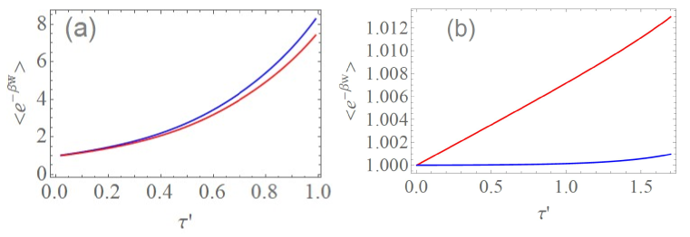
Figure S1: Comparison between the quantities $\left\langle e^{-\beta w_{\mathrm{w}}}\right\rangle$ with non-zero coupling (red line) and $e^{-\beta\Delta F_{\mathrm{w}}}$ (blue line), as a function of the work protocol duration $\tau^{\prime}$, with the initial state chosen as the Gibbs state $\Omega$. (a) shows the results in the central spin model, and the parameters are inverse temperature $\beta=1$, $\lambda_{\mathrm{x}}(0)=1$, $\lambda_{\mathrm{z}}(0)=1$, $\omega_{\mathrm{b}}=1$, $h=1$, $\alpha_{\mathrm{x}}=1$, $\alpha_{\mathrm{z}}=-0.6$, coupling strength $g=0.3$ and number of bath spins $N=6$. (b) shows the results in the Caldeira-Leggett like model, and the parameters are chosen as inverse temperature $\beta=4.08$, trapping-frequency of bath $\omega_{\mathrm{Cs}}^{\mathrm{r}}=1$, trapping-frequency of system $\omega_{\mathrm{Li}}^{\mathrm{r}}=2.83$, trapping-frequency ramping rate $\alpha=-0.1$ and coupling strength $g=0.1$.

IV Work fluctuation theorems with strong system-bath coupling

The three-stage time evolution picture makes it possible to know the exientence of work as a definite thermodynamic quantity, even when there is strong SBC. In particular, with the decomposition of the original time evolution operator into the products of three terms as shown in Eq. (S1) or Eq. (S2), work done can be entirely associated with the propagator $U_{\mathrm{uc}}$, which depicts a system without its coupling to the bath. Hence, the work with strong SBC can be investigated by checking the work done associated with $U_{\mathrm{uc}}$ for the time interval interval $[0,\tau^{\prime}]$. As also mentioned in the main text, we assume that the initial state of the work process is the Gibbs state $\Omega_{\mathrm{uc}}$ (as the result of a long self-relaxation process) and so the initial state of the system is$\ \varpi_{\mathrm{s}}(0)$, defined in the previous section, with no initial coherence between the energy eigenstates. The characteristic function of work will be exactly the same as that computed from $U_{\mathrm{uc}}$, namely, $\Theta_{0\rightarrow\tau^{\prime}}^{\mathrm{w}}(u)$. Using the expessions of work characteristic functions in the previous section and also adding the time-independent bath Hamiltinian $H_{\mathrm{b}}$, we obtain

$$\Theta_{0\rightarrow\tau^{\prime}}^{\mathrm{w}}(u)=Z(0)^{-1}\mathrm{Tr}\{U_{\mathrm{uc}}^{\dagger}e^{iu[H_{\mathrm{s}}(\tau^{\prime})+H_{\mathrm{b}}]}U_{\mathrm{uc}}e^{-iu[H_{\mathrm{s}}(0)+H_{\mathrm{b}}]}e^{-\beta[H_{\mathrm{s}}(0)+H_{\mathrm{b}}]}\},$$ (S29)

where the commutator $[U_{\mathrm{uc}},H_{\mathrm{b}}]=0$, $U_{\mathrm{uc}}=U_{t_{0}\rightarrow\tau^{\prime}}^{\mathrm{s}}e^{-iH_{\mathrm{b}}\tau^{\prime}}$ and $Z(0)=Z_{\mathrm{s}}(0)Z_{\mathrm{b}}$ with $Z_{\mathrm{b}}=\mathrm{Tr}_{\mathrm{b}}e^{-\beta H_{\mathrm{b}}}$ are used. Further using the relation $U_{\mathrm{uc}}=e^{-igG}U_{0\rightarrow\tau^{\prime}}e^{igG}$, the the above equation can be transformed to

$$\Theta_{t_{0}\rightarrow\tau^{\prime}}^{\mathrm{w}}(u) = Z(0)^{-1}\mathrm{Tr}\{e^{-igG}U_{0\rightarrow\tau^{\prime}}^{\dagger}e^{igG}e^{iu[H_{\mathrm{s}}(\tau^{\prime})+H_{\mathrm{b}}]}e^{-igG}U_{0\rightarrow\tau^{\prime}}e^{igG}e^{-iu[H_{\mathrm{s}}(0)+H_{\mathrm{b}}]}e^{-\beta[H_{\mathrm{s}}(0)+H_{\mathrm{b}}]}\}$$

$$= Z(0)^{-1}\mathrm{Tr}\{U_{0\rightarrow\tau^{\prime}}^{\dagger}e^{igG}e^{iu[H_{\mathrm{s}}(\tau^{\prime})+H_{\mathrm{b}}]}e^{-igG}U_{0\rightarrow\tau^{\prime}}e^{igG}e^{-iu[H_{\mathrm{s}}(0)+H_{\mathrm{b}}]}e^{-igG}e^{igG}e^{-\beta[H_{\mathrm{s}}(0)+H_{\mathrm{b}}]}e^{-igG}\}.$$

Through the relation $\mathcal{H}(t)=e^{igG}[H_{\mathrm{s}}(t)+H_{\mathrm{b}}]e^{-igG}$, the above characteristic function is then reduced to

$$\Theta_{0\rightarrow\tau^{\prime}}(u)=Z(0)^{-1}\mathrm{Tr}[U_{0\rightarrow\tau^{\prime}}^{\dagger}e^{iu\mathcal{H}(\tau^{\prime})}U_{0\rightarrow\tau^{\prime}}e^{-iu\mathcal{H}(0)}e^{-\beta\mathcal{H}(0)}].$$ (S31)

Note that this expression above for work characteristic function is now entirely about the original system-bath Hamiltonian $\mathcal{H}$, and hence we have arrived at a key expression for work fluctuation theorems with strong SBC. For this reason, in the equation above we have also dropped the “w” superscript.

V Work, heat and internal energy at arbitrary SBC strength

As outlined in the main text and also in previous sections, the heat exchanged in the original system with arbitrary SBC strength during the time interval $[0,\tau^{\prime}]$ can be calculated from $U_{\mathrm{w\tau^{\prime}}}$ and $U_{\mathrm{w0}}$, the two auxiliary evolution operators associated with time intervals $[-\tau,0]$ and $[\tau^{\prime},\tau+\tau^{\prime}]$, where the system-bath coupling can be understood to be vanishingly small. To focus on the differential behaviors of heat exchange, let us also assume $\tau^{\prime}$ to be infinitely small.

The total heat exchange hence occurs during the two self-relaxation time intervals $[-\tau,0]$ and $[\tau^{\prime},\tau+\tau^{\prime}]$. There is no ambuity in calculating heat during these two processes because in above we have already introduced how heat should be calculated under weak SBC. The total heat exchange is then found to be the following:

$$dQ = \int_{-\tau}^{0}\mathrm{Tr}_{\mathrm{s}}(H_{\mathrm{s}}\ d\rho_{\mathrm{s}})+\int_{\tau^{\prime}}^{\tau^{\prime}+\tau}\mathrm{Tr}_{\mathrm{s}}(H_{\mathrm{s}}\ d\rho_{\mathrm{s}})$$ (S32)

$$= \mathrm{Tr}_{\mathrm{s}}[H_{\mathrm{s}}(-\tau)\rho_{\mathrm{s}}(0)]-\mathrm{Tr}_{\mathrm{s}}[H_{\mathrm{s}}(-\tau)\rho_{\mathrm{s}}(-\tau)]+\mathrm{Tr}_{\mathrm{s}}[H_{\mathrm{s}}(\tau^{\prime})\rho_{\mathrm{s}}(\tau^{\prime}+\tau)]-\mathrm{Tr}_{\mathrm{s}}[H_{\mathrm{s}}(\tau^{\prime})\rho_{\mathrm{s}}(\tau^{\prime})],$$

where we have used, consistent with our construction, that the system $H_{\mathrm{s}}$ does not change during the time intervals $[-\tau,0]$ and $[\tau^{\prime},\tau+\tau^{\prime}]$, always fixed at either $H_{s}(0)$ or $H_{s}(\tau^{\prime})$. Further using the obvious relation $\mathrm{Tr}_{\mathrm{s}}[A_{\mathrm{s}}(t)\rho_{\mathrm{s}}(t)]=\mathrm{Tr}[A_{\mathrm{s}}(t)\rho(t)]$ with $A_{\mathrm{s}}$ being any system operator, we can reexpress this expression for heat in terms of the following:

$$dQ=\mathrm{Tr}[H_{\mathrm{s}}(-\tau)\rho(0)]-\mathrm{Tr}[H_{\mathrm{s}}(-\tau)\rho(-\tau)]+\mathrm{Tr}[H_{\mathrm{s}}(\tau^{\prime})\rho(\tau^{\prime}+\tau)]-\mathrm{Tr}[H_{\mathrm{s}}(\tau^{\prime})\rho(\tau^{\prime})].$$ (S33)

Next we wish to connect the above expression for heat with system-bath’s orginal Hamiltonian $\mathcal{H}$. This can be partially done. We first use the following relations:

$$\rho(0) = e^{-igG}\rho(-\tau)e^{igG},$$ (S34)

$$\rho(\tau^{\prime}) = U_{\mathrm{uc}}e^{-igG}\rho(-\tau)e^{igG}U_{\mathrm{uc}}^{\dagger},$$ (S35)

$$\rho(\tau^{\prime}+\tau) = e^{igG}U_{\mathrm{uc}}e^{-igG}\rho(-\tau)e^{igG}U_{\mathrm{uc}}^{\dagger}e^{-igG}.$$ (S36)

In addition, for an infinitesimal $\tau^{\prime}$, the time evolution operator$\ U_{\mathrm{uc}}\$ can be rewritten to the first order of $\tau^{\prime}$ as $U_{\mathrm{uc}}=\mathcal{T}\exp[-i\int_{0}^{\tau^{\prime}}H_{\mathrm{uc}}(s)ds]\approx 1-iH_{\mathrm{uc}}(0)\tau^{\prime}=1-iH_{\mathrm{uc}}(-\tau)\tau^{\prime}$. Putting all these considerations together, we obtain

$$dQ = \mathrm{Tr}[H_{\mathrm{s}}(-\tau)e^{-igG}\rho(-\tau)e^{igG}]-\mathrm{Tr}[H_{\mathrm{s}}(-\tau)\rho(-\tau)]$$ (S37)

$$+\mathrm{Tr}\{H_{\mathrm{s}}(\tau^{\prime})e^{igG}[1-iH_{\mathrm{uc}}(-\tau)\tau^{\prime}]e^{-igG}\rho(-\tau)e^{igG}[1+iH_{\mathrm{uc}}(-\tau)\tau^{\prime}]e^{-igG}\}$$

$$-\mathrm{Tr}\{H_{\mathrm{s}}(\tau^{\prime})[1-iH_{\mathrm{uc}}(-\tau)\tau^{\prime}]e^{-igG}\rho(-\tau)e^{igG}[1+iH_{\mathrm{uc}}(-\tau)\tau^{\prime}]\}.$$

To the first order of the time $\tau^{\prime}$, this expression of heat can be rearranged to become

$$dQ = \mathrm{Tr}\{H_{\mathrm{s}}(-i)[e^{igG}H_{\mathrm{uc}}(-\tau)e^{-igG},\rho]\tau^{\prime}\}$$ (S38)

$$+\mathrm{Tr}(\rho dH_{\mathrm{s}})-\mathrm{Tr}[e^{igG}(dH_{\mathrm{s}})e^{-igG}\rho],$$

where $H_{\mathrm{s}}=H_{\mathrm{s}}(-\tau)=H_{\mathrm{s}}(0)$, $dH_{\mathrm{s}}=H_{\mathrm{s}}(\tau^{\prime})-H_{\mathrm{s}}(-\tau)=H_{\mathrm{s}}(\tau^{\prime})-H_{\mathrm{s}}(0)$ and we have denoted the very initial density of the whole system-bath system $\rho(-\tau)$ as $\rho$. Noting that the infinitesimal state evolution under the whole system-bath Hamiltonian $\mathcal{H=}e^{iG}H_{\mathrm{uc}}(-\tau)e^{-iG}$ is actually $d\rho=-i[\mathcal{H},\rho(-\tau)]\tau^{\prime}$, we finally have

$$dQ = \mathrm{Tr}(H_{\mathrm{s}}\ d\rho)+\mathrm{Tr}[\rho\ d(H_{\mathrm{s}}-e^{igG}H_{\mathrm{s}}e^{-igG})]$$ (S39)

$$= \mathrm{Tr}(H_{\mathrm{s}}\ d\rho)+\mathrm{Tr}\{\rho\ d[H_{\mathrm{s}}-e^{igG}(H_{\mathrm{s}}+H_{\mathrm{b}})e^{-igG}]\}$$

$$= \mathrm{Tr}_{\mathrm{s}}(H_{\mathrm{s}}\ d\rho_{\mathrm{s}})+\mathrm{Tr}[\rho\ d(H_{\mathrm{s}}-\mathcal{H})],$$

where the time-independent Hamiltonian of the bath $d(e^{igG}H_{\mathrm{b}}e^{-igG})=0$ is used, and $d\rho_{\mathrm{s}}=\mathrm{Tr}_{\mathrm{b}}(d\rho)$. This is the expression presented in the main text. Note that this expression of heat is markedly different from the previous expression $dQ_{\mathrm{w}}$ under weak SBC. To obtain $dQ$, one not only needs to know the change in the reduced density of the system, as what we normally need in cases of weak SBC, but also need to examine the second term in Eq. (S39) that involves $H_{\mathrm{s}}$.

Having derived the heat expression, we now turn to work, which can be investigated by focusing on the time interval $[0,\tau^{\prime}]$ in our three-stage picture. During this stage, the system and bath is uncoupled. Thus, the work done, denoted $dW$, can be calculated by examining the internal energy change to the system $H_{s}$. That is,

$$dW = \mathrm{Tr}_{\mathrm{s}}[\rho_{\mathrm{s}}(\tau^{\prime})H_{\mathrm{s}}(\tau^{\prime})]-\mathrm{Tr}_{\mathrm{s}}[\rho_{\mathrm{s}}(0)H_{\mathrm{s}}(0)]$$ (S40)

$$= \mathrm{Tr}[\rho(\tau^{\prime})H_{\mathrm{uc}}(\tau^{\prime})]-\mathrm{Tr}[\rho(0)H_{\mathrm{uc}}(0)],$$

where, consistent with our treatment, we have assumed that $H_{\mathrm{b}}$ as part of $H_{\mathrm{uc}}$ is time independent. As in treating heat exchange above, let us now rewrite both the states $\rho(0)$ and $\rho(\tau^{\prime})$ in terms of the initial state $\rho(-\tau)$ through $\rho(0)=e^{-igG}\rho(-\tau)e^{igG}$ and $\rho(\tau^{\prime})=U_{\mathrm{uc}}e^{-igG}\rho(-\tau)e^{igG}U_{\mathrm{uc}}^{\dagger}$. Furthe considering an infinitemal $\tau^{\prime}$ to capture the differential work $dW$, we safely use the expansion $U_{\mathrm{uc}}\approx 1-iH_{\mathrm{uc}}(0)\tau^{\prime}$ to the first order of time $\tau^{\prime}$. This leads us to

$$dW = \mathrm{Tr}\{\rho(-\tau)e^{igG}[1+iH_{\mathrm{uc}}(0)\tau^{\prime}][H_{\mathrm{uc}}(0)+(\partial_{t}H_{\mathrm{uc}})\tau^{\prime}][1-iH_{\mathrm{uc}}(0)\tau^{\prime}]e^{-igG}\}$$ (S41)

$$-\mathrm{Tr}[\rho(-\tau)e^{igG}H_{\mathrm{uc}}(0)e^{-igG}]$$

$$= \mathrm{Tr}[\rho(-\tau)e^{igG}(\partial_{t}H_{\mathrm{uc}})\tau^{\prime}e^{-igG}],$$

where $(\partial_{t}H_{\mathrm{uc}})\tau^{\prime}=dH_{\mathrm{uc}}$ represents the infinitesimal change in the Hamiltonian $H_{\mathrm{uc}}$: $H_{\mathrm{uc}}(\tau^{\prime})-H_{\mathrm{uc}}(0)$. Finally, using the relation $\mathcal{H=}e^{igG}H_{\mathrm{uc}}e^{-igG}$, the $dW$ expression reduces to

$$dW=\mathrm{Tr}(\rho\ d\mathcal{H}).$$ (S42)

This is the expression presented in the main text.

It now becomes interesting to check what happens to the energy throughout the whole process that is digested in terms of three stages. For convenience we still assume $\tau^{\prime}$ to be infinitesimal. The total internal energy change, caused by heat exchange and work done, must be given by

$$dE=\mathrm{Tr}_{\mathrm{s}}[\rho_{\mathrm{s}}(\tau+\tau^{\prime})H_{\mathrm{s}}(\tau+\tau^{\prime})-\rho_{\mathrm{s}}(-\tau)H_{\mathrm{s}}(-\tau)].$$ (S43)

With the obvious relation $\mathrm{Tr}_{\mathrm{s}}[H_{\mathrm{s}}(t)\rho_{\mathrm{s}}(t)]=\mathrm{Tr}[H_{\mathrm{s}}(t)\rho(t)]$, we can rewrite $dE$ as the following:

$$dE=\mathrm{Tr}[\rho(\tau+\tau^{\prime})H_{\mathrm{s}}(\tau+\tau^{\prime})-\rho(-\tau)H_{\mathrm{s}}(-\tau)].$$ (S44)

Again, if we now rewrite $\rho(\tau+\tau^{\prime})$ in terms of $\rho(-\tau)$, with

$$\rho(\tau+\tau^{\prime})=e^{igG}U_{\mathrm{uc}}e^{-igG}\rho(-\tau)e^{igG}U_{\mathrm{uc}}^{\dagger}e^{-igG}\approx e^{igG}[1-iH_{\mathrm{uc}}(-\tau)\tau^{\prime}]e^{-igG}\rho(-\tau)e^{igG}[1+iH_{\mathrm{uc}}(-\tau)\tau^{\prime}]e^{-igG}$$ (S45)

to the first order of $\tau^{\prime}$, we arrive at

$$dE = \mathrm{Tr}\{H_{\mathrm{s}}(\tau^{\prime})e^{igG}[1-iH_{\mathrm{uc}}(-\tau)\tau^{\prime}]e^{-igG}\rho(-\tau)e^{igG}[1+iH_{\mathrm{uc}}(-\tau)\tau^{\prime}]e^{-igG}\}-\mathrm{Tr}[\rho(-\tau)H_{\mathrm{s}}(-\tau)].$$

$$= \mathrm{Tr}\{[H_{\mathrm{s}}(\tau^{\prime})-H_{\mathrm{s}}(0)]\rho(-\tau)]\}-i\mathrm{Tr}\{H_{\mathrm{s}}(\tau^{\prime})[e^{igG}H_{\mathrm{uc}}(-\tau)e^{-igG},\rho(-\tau)]\}\tau^{\prime}$$

$$= \mathrm{Tr}(\rho\ dH_{\mathrm{s}})+\mathrm{Tr}(H_{\mathrm{s}}\ d\rho)$$

Comparing with expressions of $dW$ and $dQ$ in Eq. (S42) and  (S39), one immediately observes

$$dE=dW+dQ.$$

This can be understood as the manifestion of the first law of quantum thermodynamics in our treatment.

In Fig. S2 (a), (b), (d) and (e) we compare the basic quantities between weak and strong SBC for both the central spin model and Caldeira-Leggett like model. Similar to a trend observed in Fig. S1, it is seen that the difference is more apparent when the duration of the work protocol increases, namely, a larger $\tau^{\prime}$.

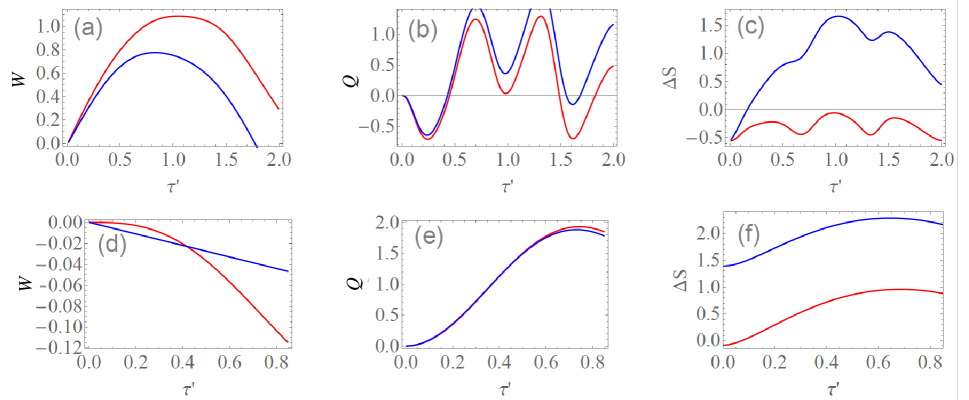
Figure S2: Comparison in thermodynamics quantities between strong SBC (blue lines) and weak SBC (red lines) as a function of the duration of the work protocol $\tau^{\prime}$. (a), (b) and (c), respectively, show $W$, $Q$ and $\Delta S$ as a function of time for central spin model, and (d), (e) and (f) are to compare the same but for the Caldeira-Leggett like model. The corresponding parameters are the same as those in Fig. S1.

VI The entropy at strong coupling

To obtain the entropy, first, we define thermodynamic entropy as $dS=\beta dQ$, if and only if the process is quasi-static. Here as the presence of bath, the quasi-static means that the composite system can always be maintained in the global Gibbs state $\Omega$ [8]. With the definition of heat $dQ=\mathrm{Tr}(H_{\mathrm{s}}\ d\rho)+\mathrm{Tr}[\rho\ d(H_{\mathrm{s}}-\mathcal{H})]$, we obtain

$$dS=-d\mathrm{Tr}(\Omega_{\mathrm{s}}\ln\varpi_{\mathrm{s}})-\mathrm{Tr}(\Omega d\ln\Omega)-d\ln\frac{Z_{\mathrm{s}}}{Z},$$ (S47)

where the state of the composite system $\rho$ is replaced by the Gibbs state $\Omega$, and the reduced state of the system is $\Omega_{\mathrm{s}}=\mathrm{Tr}_{\mathrm{b}}\Omega$. From the definition of partition function the following relation $Z(t)=\mathrm{Tr}[e^{-\beta\mathcal{H}(t)}]=\mathrm{Tr}[e^{igG}e^{-\beta H_{\mathrm{uc}}(t)}e^{-igG}]=\mathrm{Tr}[e^{-\beta H_{\mathrm{uc}}(t)}]=Z_{\mathrm{s}}(t)Z_{\mathrm{b}}$ can be obtained, and then the quantity $\frac{Z(t)}{Z_{\mathrm{s}}(t)}=Z_{\mathrm{b}}$ is time-independent. Then the last term is zero, i.e., $d\ln\frac{Z_{\mathrm{s}}}{Z}=0$. Also as $\mathrm{Tr}(\Omega d\ln\Omega)=d\mathrm{Tr}(\Omega)=0$, the entropy is reduced to

$$dS=-d\mathrm{Tr}(\Omega_{\mathrm{s}}\ln\varpi_{\mathrm{s}}).$$ (S48)

With the definition of relative entropy, the change of thermodynamic entropy is transformed to

$$dS=dS_{v}(\Omega_{\mathrm{s}})+dD(\left.\Omega_{\mathrm{s}}\right|\varpi_{\mathrm{s}}),$$ (S49)

where the von Neumann entropy is $S_{v}(\Omega_{\mathrm{s}})=-\mathrm{Tr}_{\mathrm{s}}(\Omega_{\mathrm{s}}\ln\Omega_{\mathrm{s}})$, and the relative entropy is $D(\left.\Omega_{\mathrm{s}}\right|\varpi_{\mathrm{s}})=\mathrm{Tr}_{\mathrm{s}}[\Omega_{\mathrm{s}}\ln\Omega_{\mathrm{s}}]-\mathrm{Tr}_{\mathrm{s}}[\Omega_{\mathrm{s}}\ln\varpi_{\mathrm{s}}]$. Fig. S2 (c) and (f) show the difference with that at weak coupling. Being different from work and heat, the difference may arise at the very start of the work protocol, because the entropy is a state variable.

VII Details of the relation $\Delta F=\Delta E-T\Delta S$

With the definition of free energy $F=T\ln Z_{\mathrm{s}}$ and the partition function of system $Z_{\mathrm{s}}(t)=\mathrm{Tr}_{\mathrm{s}}\{\exp[-\beta H_{\mathrm{s}}(t)]\}$, the change of free energy is

$$dF=-T\ln Z_{\mathrm{s}}(\tau^{\prime}+\tau)+T\ln Z_{\mathrm{s}}(-\tau).$$ (S50)

As mentioned in maintext, in both time intervals $[-\tau,0$] and $[\tau^{\prime},\tau+\tau^{\prime}]$, heat is transferred while no work protocol is executed via any change in the system parameters (given that the Hamiltonians of the system is viewed as unchanged in these two time intervals). Hence, the free energies are also unchanged in these time intervals, and the free energy change can then be rewritten as

$$dF=-T\ln Z_{\mathrm{s}}(\tau^{\prime})+T\ln Z_{\mathrm{s}}(0).$$ (S51)

Since the Hamiltonian of the bath is time independent, its free energy is a constant. As a result, the free energy change can be transformed to

$$dF = -T\ln\mathrm{Tr}_{\mathrm{s}}\{e^{-\beta[H_{\mathrm{s}}(0)+dH_{\mathrm{s}}]}\}-T\ln\mathrm{Tr}_{\mathrm{b}}(e^{-\beta H_{\mathrm{b}}})+T\ln\mathrm{Tr}_{\mathrm{s}}[e^{-\beta H_{\mathrm{s}}(0)}]+T\ln\mathrm{Tr}_{\mathrm{b}}(e^{-\beta H_{\mathrm{b}}})$$ (S52)

$$= -T\ln\mathrm{Tr}\{e^{-\beta[H_{\mathrm{s}}(0)+dH_{\mathrm{s}}+H_{\mathrm{b}}]}\}+T\ln\mathrm{Tr}\{e^{-\beta[H_{\mathrm{s}}(0)+H_{\mathrm{b}}]}\},$$

where time $\tau^{\prime}$ is infinitely small, and the Hamiltonian is rewritten as $H_{\mathrm{s}}(\tau^{\prime})=H_{\mathrm{s}}(0)+dH_{\mathrm{s}}$. The free energy change is then reduced to

$$dF = -T\ln\mathrm{Tr}\{e^{-\beta[H_{\mathrm{s}}(0)+H_{\mathrm{b}}]}(1-\beta dH_{\mathrm{s}})\}+T\ln\mathrm{Tr}\{e^{-\beta[H_{\mathrm{s}}(0)+H_{\mathrm{b}}]}\}$$ (S53)

$$= \mathrm{Tr}[\varpi(0)d(H_{\mathrm{s}}+H_{\mathrm{b}})],$$

where the time-independent Hamiltonian of the bath is used. Finally, we note that $\varpi(0)=e^{-igG}\rho(-\tau)e^{igG}$ after assuming that the initial state is the Gibbs state $\rho(-\tau)=\Omega(-\tau)$. As such, we can further rewrite $dF$ as the following:

$$dF = \mathrm{Tr}[e^{-igG}\rho(-\tau)e^{igG}d(H_{\mathrm{s}}+H_{\mathrm{b}})]$$ (S54)

$$= \mathrm{Tr}(\rho\ d\mathcal{H}),$$

where $\mathcal{H}=e^{igG}(H_{\mathrm{s}}+H_{\mathrm{b}})e^{-igG}$ is used. This is consistent with our work expression since during a quasi-static process at constant temperature, $dF$ is expected to be the same as $dW$. Finally, combining with Eqs (S42) and (S47) the relation $\Delta F=\Delta E-T\Delta S$ mentioned in the main text can be obtained.

References

[1] J. G. Kirkwood, Statistical mechanics of fluid mixtures,
J. Chem. Phys. 3, 300 (1935).
[2] P. Strasberg and M. Esposito, Stochastic thermodynamics
in the strong coupling regime: An unambiguous approach based on coarse
graining, Phys. Rev. E 95, 062101 (2017).
[3] U. Seifert, First and second law of thermodynamics at
strong coupling, Phys. Rev. Lett. 116, 020601 (2016).
[4] C. Jarzynski, Nonequilibrium work theorem for a system
strongly coupled to a thermal environment. J. Stat. Mech. P09005 (2004).
[5] M. Rigol, V. Dunjko, M. Olshanii, Thermalization and its
mechanism for generic isolated quantum systems. Nature 452, 854 (2008).
[6] M. Campisi, P. Talkner, and P. Hänggi, Fluctuation
Theorem for Arbitrary Open Quantum Systems, Phys. Rev. Lett. 102, 210401
(2009).
[7] P. Strasberg, Repeated interactions and quantum stochastic
thermodynamics at strong coupling, Phys. Rev. Lett. 123, 180604 (2019).
[8] M. Campisi, P. Talkner, and P. Hänggi, Fluctuation
Theorem for Arbitrary Open Quantum Systems. Phys. Rev. Lett. 102, 210401
(2009).
[9] M. Perarnau-Llobet, H. Wilming, A. Riera, R. Gallego, and
J. Eisert, Strong coupling corrections in quantum thermodynamics, Phys. Rev.
Lett. 120, 120602 (2018).
[10] A. Colla and H. P. Breuer, Open-system approach to
nonequilibrium quantum thermodynamics at arbitrary coupling, Phys. Rev. A
105, 052216 (2022).
[11] F. Ivander, N. A. Sztrikacs and D. Segal, Strong
system-bath coupling effects in quantum absorption refrigerators, Phys. Rev.
E 105, 034112 (2022).
[12] P. Strasberg and M. Esposito, Non-Markovianity and
negative entropy production rates, Phys. Rev. E 99, 012120 (2019).
[13] Á Rivas, Strong Coupling Thermodynamics of Open Quantum
Systems, Phys. Rev. Lett. 124, 160601 (2020).
[14] U. Weiss, Quantum Dissipative Systems, Series in Modern
Condensed Matter Systems (Scientific, Singapore) (2008).
[15] P. Lambropoulos, G. M. Nikolopoulos, T. R. Nielsen,
and S. Bay, Fundamental quantum optics in structured reservoirs, Rep. Prog.
Phys. 63, 455 (2000).
[16] N. Lambert, Y.-N. Chen, Y.-C. Cheng, C.-M. Li, G.-Y. Chen,
and F.Nori, Quantum biology, Nat. Phys. 9, 10 (2013).
[17] C. K. Lee, J. S. Cao and J. B. Gong, Non-Canonical
Statistics of a Spin-Boson Model: Theory and Exact Monte-Carlo Simulations.
Phys. Rev. E. 86, 021109 (2012).
[18] Y. Ashida, A. İmamoğlu, and E. Demler, Cavity
quantum electrodynamics at arbitrary light-matter coupling strengths, Phys.
Rev. Lett. 126, 153603 (2021).
[19] T. D. Lee, F. E. Low, and D. Pines, The motion of slow
electrons in a polar crystal, Phys. Rev. 90, 297 (1953).
[20] I. de Vega and D. Alonso, Dynamics of non-Markovian open
quantum systems, Rev. Mod. Phys. 89, 015001 (2017).
[21] A. O. Caldeira and A. J. Leggett, Path integral approach
to quantum Brownian motion, Physica A 121, 587 (1983).
[22] Supplemental Material
[23] R. Alicki, The quantum open system as a model of the heat
engine. J. Phys. A: Math. General 12(5), L103 (1979).
[24] P. Talkner, E. Lutz, P. Hänggi, Fluctuation theorems:
Work is not an observable, Phys. Rev. E 75, 050102(R) (2007).
[25] M. Campisi, P. Hänggi, and P. Talkner, Quantum
fluctuation relations: Foundations and applications, Rev. Mod. Phys. 83, 771
(2011).
[26] M. Esposito, U. Harbola, and S. Mukamel, Nonequilibrium
fluctuations, fluctuation theorems, and counting statistics in quantum
systems, Rev. Mod. Phys. 81, 1665 (2009).
[27] J. Kurchan, A quantum fluctuation theorem,
arXiv:cond-mat/0007360 (2000); H. Tasaki, Jarzynski Relations for Quantum
Systems and Some Applications, arXiv:cond-mat/0009244 (2000).
[28] P. Talkner and P. Hänggi, The Tasaki-Crooks quantum
fluctuation theorem, J. Phys. A 40, F569 (2007).
[29] The interaction Hamiltonian is quenched at the time
and , and then there are some work added for finite time
interval . These two work will approach to zero in the limit , as the work induced by quenching is .
[30] G. Y. Xiao and J. B. Gong, Principle of Minimal Work
Fluctuations, Physical Review E 92, 022130 (2015).
[31] H. T. Quan, Z. Song, X. F. Liu, P. Zanardi, and C. P. Sun,
Decay of Loschmidt Echo Enhanced by Quantum Criticality, Phys. Rev. Lett.
96, 140604 (2006).
[32] Takahashi, M., Thermodynamics of One-Dimensional
Solvable Models Cambridge University Press, Cambridge, England (1999).
[33] The absolute difference and are
defined, respectively, as
and , where the quantities
under weak SBC are and with the state chosen as the reduced state of the system coupled to its
bath.

References

[1] R. Onofrio and B. Sundaram, Effective
microscopic models for sympathetic cooling of atomic gase, Phys. Rev. A 92,
033422 (2015).
[2] M. Mudrich, S. Kraft, K. Singer, R. Grimm, A. Mosk, and M.
Weidemüller, Sympathetic Cooling with Two Atomic Species in an Optical
Trap, Phys. Rev. Lett. 88, 253001 (2002).
[3] G. Modugno, G. Ferrari, G. Roati, R. J. Brecha, A. Simoni,
M. Inguscio, Bose-Einstein Condensation of Potassium Atoms by Sympathetic
Cooling, Science 294, 1320 (2001).
[4] H. Engler, T. Weber, M. Mudrich, R. Grimm, and M. Weidemüller, Very long storage times and evaporative cooling of cesium atoms
in a quasielectrostatic dipole trap, Phys. Rev. A 62, 031402(R) (2000).
[5] R. Alicki, The quantum open system as a model of the heat
engine. J. Phys. A: Math. General 12(5), L103 (1979).
[6] J. Kurchan, A quantum fluctuation theorem,
arXiv:cond-mat/0007360 (2000); H. Tasaki, Jarzynski Relations for Quantum
Systems and Some Applications, arXiv:cond-mat/0009244 (2000).
[7] P. Talkner and P. Hänggi, The Tasaki-Crooks quantum
fluctuation theorem, J. Phys. A 40, F569 (2007).
[8] J. D. Cresser and J. Anders, Weak and Ultrastrong
Coupling Limits of the Quantum Mean Force Gibbs State, Phys. Rev. Lett. 127,
250601 (2021).