Analysis of Interpolating Regression Models and the Double Descent Phenomenon

Abstract

A regression model with more parameters than data points in the training data is overparametrized and has the capability to interpolate the training data. Based on the classical bias-variance tradeoff expressions, it is commonly assumed that models which interpolate noisy training data are poor to generalize. In some cases, this is not true. The best models obtained are overparametrized and the testing error exhibits the double descent behavior as the model order increases. In this contribution, we provide some analysis to explain the double descent phenomenon, first reported in the machine learning literature. We focus on interpolating models derived from the minimum norm solution to the classical least-squares problem and also briefly discuss model fitting using ridge regression. We derive a result based on the behavior of the smallest singular value of the regression matrix that explains the peak location and the double descent shape of the testing error as a function of model order.

1 Introduction

Linearly parametrized regression models that interpolate the training data have recently attracted significant attention [3], mainly due to the close connections to many state-of-the-art machine learning models [10, 1]. Interpolation of the training data is obtained when the number of estimated/trained parameters in the model is equal to or larger than the number of training data used to estimate the model. Such models are hence overparametrized and there exists an infinite number of solutions that interpolate the data. It has been noticed in recent publications [3, 8] that the quality of an estimated model with a linear parametrization often follows a so-called double descent curve. This means that the test data error first decreases with an increasing model order and then increases again to a maximum when the number of samples of the data is equal to the number of parameters and then gradually decreases again with an increasing model order. The double descent phenomenon has previously been noticed in the deep-learning area [1, 7].

In this paper, we will show that this behavior can be explained with a minimum of theory and complement the available literature on the subject. Furthermore, we point out that the extent of the behavior is closely tied to how the model class is constructed, i.e., the ordering of the basis functions employed in the regression model.

The paper is structured as follows. In Section 2, the regression problem is formulated and necessary notation and assumptions are explained. In Section 3, we derive explicit expressions for the bias and variance contributions for predictions obtained using the estimated model and show that the smallest singular value of the regression matrix plays a key role. We further provide a theorem that predicts the behavior of the smallest singular value as the model order increases. A few numerical examples are given in Section 4 that illustrate the connection between the model quality and the smallest singular value. In Section 5, the paper is concluded with a summary of the findings.

2 Problem formulation

We consider a general regression problem where we seek a function that maps a value in the domain $\mathcal{X}$ to the co-domain $\mathcal{Y}$, i.e. $f:\mathcal{X}\rightarrow\mathcal{Y}$ based on a given set of samples of training data

$$\mathcal{D}=\{(y(t),x(t))\}_{t=1}^{M}$$ (1)

where $x(t)\in\mathcal{X}$ and $y(t)\in\mathcal{Y}$ and we consider a linearly parametrized function class

$$f(x;\bm{\theta})=\sum_{i=1}^{n}\theta_{i}\phi_{i}(x)=\bm{\phi}(x)\bm{\theta}$$ (2)

where $\phi_{i}:\mathcal{X}\rightarrow\mathcal{Y}$ are given distinct basis functions and

$$\bm{\phi}(x) =\begin{bmatrix}\phi_{1}(x)&\phi_{2}(x)&\cdots&\phi_{n}(x)\end{bmatrix}$$ (3)

$$\bm{\theta} =\begin{bmatrix}\theta_{1}&\theta_{2}&\cdots&\theta_{n}\end{bmatrix}^{T}\in\mathcal{T}.$$

The model order is equal to the size of the parameter vector $\bm{\theta}$ and is denoted by the integer $n$. In the analysis that follows we assume the sets $\mathcal{X}$ and $\mathcal{Y}$ can be real or complex spaces with finite dimensions $m$ and $p$ respectively and the parameter set $\mathcal{T}$ can be real or complex valued with finite dimension $n$.

Based on the training data set the model parameters are determined by minimizing the sum of squared errors

$$\hat{\bm{\theta}}=\arg\min_{\bm{\theta}}\sum_{t=1}^{M}\|y(t)-\sum_{i=1}^{n}\theta_{i}\phi_{i}(x(t))\|^{2}$$ (4)

The minimization problem above can be written as the least-squares (LS) problem

$$\hat{\bm{\theta}}=\arg\min_{\bm{\theta}}\|\bm{y}-\bm{\Phi}\bm{\theta}\|^{2}$$ (5)

with the regression matrix

$$\bm{\Phi}=\begin{bmatrix}\bm{\phi}(x(1))\\ \bm{\phi}(x(2))\\ \vdots\\ \bm{\phi}(x(M))\\ \end{bmatrix}=\begin{bmatrix}\phi_{1}(x(1))&\phi_{2}(x(1))&\cdots&\phi_{n}(x(1))\\ \phi_{1}(x(2))&\phi_{2}(x(2))&\cdots&\phi_{n}(x(2))\\ \vdots&\vdots&\vdots&\vdots\\ \phi_{1}(x(M))&\phi_{2}(x(M))&\cdots&\phi_{n}(x(M))\\ \end{bmatrix}$$ (6)

which is a matrix with $N\triangleq pM$ rows and $n$ columns and the vector

$$\bm{y}=\begin{bmatrix}y(1)\\ y(2)\\ \vdots\\ y(M)\end{bmatrix}.$$ (7)

has $N$ elements. We note that if $n\leq N$ we have an under-parametrized problem and the solution to (5) is unique if $\mathbf{\Phi}$ has full rank. If $n>N$ the problem is overparametrized and there exist infinite many solutions to (5). The singular value decomposition (SVD) [2] of the regression matrix $\mathbf{\Phi}$ in (3) plays a key role in the analysis in this paper and we denote it as

$$\mathbf{\Phi}=\sum_{k=1}^{r}\sigma_{k}\bm{u}_{k}\bm{v}_{k}^{H}$$ (8)

where $r=\min(n,N)$, the ordered singular values are $\sigma_{1}\geq\sigma_{2}\geq\ldots\geq\sigma_{r}\geq 0$, and $\bm{u}_{k}$ and $\bm{v}_{k}$ are the left and right singular vectors respectively and $(\cdot)^{H}$ denote the Hermitian transpose. We assume $\bm{\Phi}$ has full rank and hence $\sigma_{r}>0$.

For analysis purposes we assume there exists a function $f_{0}:\mathcal{X}\rightarrow\mathcal{Y}$ such that the data generated can be described as

$$y(t)=f_{0}(x(t))+z(t)$$ (9)

where $z(t)$ is an i.i.d. zero mean white noise process with variance

$$\mathbf{E}\,z(t)z(t)^{H}\triangleq\bm{R}_{z}.$$

3 Analysis

In this section, we discuss and provide some analytical results on the bias and variance of the estimated model that is given by the minimum norm solution and the ridge regression solution. We show that the largest variance contribution is proportional to $1/\sigma_{r}^{2}$, the inverse of the square of the smallest singular value of the regression matrix $\bm{\Phi}$. Finally, we show that when $n<N$ and the model order is increased to $n+1$ the smallest singular value will decrease or stay unchanged. This implies that the variance increases or stays constant with the increase of the model order. Furthermore, when $n\geq N$ and the model order is increased to $n+1$ we show that the smallest singular value is increased or stays the same. This implies that the variance decreases or stays constant with an increase in the model order.

3.1 The minimum norm solution

The unique minimum norm solution to (5) is obtained with the Moore-Penrose pseudo-inverse and can be expressed using the SVD as (see, e.g.  [2, 6])

$$\bm{\hat{\theta}}=\bm{\Phi}^{+}\bm{y}=\sum_{k=1}^{r}\frac{1}{\sigma_{k}}\bm{v}_{k}\bm{u}_{k}^{H}\bm{y}.$$ (10)

By introducing the notation

$$\bm{x}=\begin{bmatrix}x(1)\\ x(2)\\ \vdots\\ x(M)\end{bmatrix},\;\bm{f}_{0}(\bm{x})=\begin{pmatrix}f_{0}(x(1))\\ f_{0}(x(2))\\ \vdots\\ f_{0}(x(M))\end{pmatrix},\;\bm{z}=\begin{pmatrix}z(1)\\ z(2)\\ \vdots\\ z(M)\end{pmatrix}$$ (11)

the estimate in (10) can be decomposed into

$$\bm{\hat{\theta}}=\sum_{k=1}^{r}\frac{1}{\sigma_{k}}\bm{v}_{k}\bm{u}_{k}^{H}(\bm{f}_{0}(\bm{x})+\bm{z})=\bm{\theta}_{*}+\tilde{\bm{\theta}}$$ (12)

where $\bm{\theta}_{*}=\bm{\Phi}^{+}\bm{f}_{0}(\bm{x})=\sum_{k=1}^{r}\frac{1}{\sigma_{k}}\bm{v}_{k}\bm{u}_{k}^{H}\bm{f}_{0}(\bm{x})$ is the noise free minimum norm solution and $\tilde{\bm{\theta}}=\sum_{k=1}^{r}\frac{1}{\sigma_{k}}\bm{v}_{k}\bm{u}_{k}^{H}\bm{z}$ is the contribution due to the noise. The zero mean assumption on $z(t)$ yields

$$\mathbf{E}\,\bm{\hat{\theta}}=\bm{\theta}_{*}$$ (13)

The error of the output $f(x^{\prime};\hat{\bm{\theta}})$ of the estimated model given a new test data sample $x^{\prime}$ is

$$e(x^{\prime}) =\bm{\phi}(x^{\prime})\hat{\bm{\theta}}-f_{0}(x^{\prime})$$ (14)

$$=\bm{\phi}(x^{\prime})\bm{\theta}_{*}-f_{0}(x^{\prime})+\bm{\phi}(x^{\prime})\sum_{k=1}^{r}\frac{1}{\sigma_{k}}\bm{v}_{k}\bm{u}_{k}^{H}\bm{z}$$

From above it is clear that the error $e(x^{\prime})$ is composed of a bias part $\bm{\phi}(x^{\prime})\bm{\theta}_{*}-f_{0}(x^{\prime})$ and a zero mean stochastic part $\bm{\phi}(x^{\prime})\sum_{k=1}^{r}\frac{1}{\sigma_{k}}\bm{v}_{k}\bm{u}_{k}^{H}\bm{z}$ that contributes with variance

$$R_{e}(x^{\prime})\triangleq\operatorname{cov}(e(x^{\prime}))=$$ (15)

$$\bm{\phi}(x^{\prime})\left[\sum_{k=1}^{r}\frac{1}{\sigma_{k}}\bm{v}_{k}\bm{u}_{k}^{H}\right](I_{N}\otimes R_{z})\left[\sum_{k=1}^{r}\frac{1}{\sigma_{k}}\bm{v}_{k}\bm{u}_{k}^{H}\right]^{H}\bm{\phi}^{H}(x^{\prime})$$

If the measurement noise is uncorrelated between the channels and have equal variance $r_{z}$, then $R_{z}=r_{z}\bm{I}$. In this case, the covariance expression (15) is simplified to

$$R_{e}(x^{\prime}) =r_{z}\sum_{k=1}^{r}\frac{1}{\sigma^{2}_{k}}(\bm{\phi}(x^{\prime})\bm{v}_{k})(\bm{\phi}(x^{\prime})\bm{v}_{k})^{H}$$ (16)

$$=r_{z}\bm{\phi}(x^{\prime})\left(\sum_{k=1}^{r}\frac{1}{\sigma^{2}_{k}}\bm{v}_{k}\bm{v}_{k}^{H}\right)\bm{\phi}(x^{\prime})^{H}$$

since $\bm{u}_{k}^{H}\bm{u}_{l}=0$ for $k\not=l$. From (14) (and (16)) it is clear that if the smallest singular value of $\bm{\Phi}$ is close to zero the error (and variance) can become arbitrarily large unless $\bm{\phi}(x^{\prime})$ is perpendicular to the right singular vector corresponding to the smallest singular value. Further we note that for any singular value distribution we have the inequality $\sum_{k=1}^{r}\frac{1}{\sigma_{k}^{2}}\geq\frac{r^{2}}{\sum_{k=1}^{r}\sigma_{k}^{2}}$ with equality if all singular values are equal, see e.g. [9]. A selection of basis functions that results in equal singular values can hence be regarded as variance optimal.

3.2 Bias

The size of the bias contribution $\bm{\phi}(x^{\prime})\bm{\theta}_{*}-f_{0}(x^{\prime})$ in (14) depends on several factors. If we start by assuming that the model is correctly specified, i.e.  there exists a vector $\bm{\theta}_{0}$ such that for all $x$ we have $f_{0}(x)=\bm{\phi}(x)\bm{\theta}_{0}$ then the bias part of the error is

$$\mathbf{E}\,e(x^{\prime}) =\bm{\phi}(x^{\prime})\bm{\theta}_{*}-f_{0}(x^{\prime})=\bm{\phi}(x^{\prime})\bm{\Phi}^{+}\bm{\Phi}\bm{\theta}_{0}-f_{0}(x^{\prime})$$ (17)

$$=\bm{\phi}(x^{\prime})(\bm{\Phi}^{+}\bm{\Phi}-\bm{I})\bm{\theta}_{0}$$

• In the underparametrized case $(n\leq N)$, we see that $\bm{\Phi}^{+}\bm{\Phi}-\bm{I}=0$, since $\bm{\Phi}$ has full rank, thus the bias is zero.

• If $n>N$ then $\bm{\Phi}^{+}\bm{\Phi}-\bm{I}$ is a rank $n-N$ projection matrix which projects onto the nullspace of $\bm{\Phi}$. The bias of $e(x^{\prime})$ hence depends on the co-linearity of the projected true parameter vector and the row vector(s) $\bm{\phi}(x^{\prime})$. It also follows that the bias is zero if $\bm{\theta}_{0}=\bm{\Phi}^{T}\bm{p}$ for some vector $\bm{p}$. In effect, this tells us that of all possible correctly specified models $f_{0}(x)=\bm{\phi}(x)\bm{\theta}_{0}$ only the $N$ dimensional subset of models given by a parameter that can be expressed as $\bm{\Phi}^{T}\bm{p}$ will have zero bias since $(\bm{\Phi}^{+}\bm{\Phi}-\bm{I})\bm{\Phi}^{T}\bm{p}=0$. The set of zero bias models hence depends explicitly on the training data through the properties of the matrix $\bm{\Phi}$. As $n$ increases the size of the set of true functions with a non-zero bias also increases as the size of the nullspace of $\bm{\Phi}$ increases with $n$.

For the misspecified case, when true function $f_{0}(x)$ is not part of the parametrized model class $f(x;\hat{\bm{\theta})}=\bm{\phi}(x)\bm{\theta}$ the bias is

$$\mathbf{E}\,e(x^{\prime})=\bm{\phi}(x^{\prime})\bm{\theta}_{*}-f_{0}(x^{\prime})=\bm{\phi}(x^{\prime})\bm{\Phi}^{+}\bm{f}_{0}(\bm{x})-f_{0}(x^{\prime})$$ (18)

For the overparametrized case when $n\geq N$ the estimated model interpolates the training data. Hence, if $x^{\prime}$ is very close to one of the training data inputs $x(t)$ in $\mathcal{D}$, (see (1)), we can expect the bias $\mathbf{E}\,e(x^{\prime})$ to be very small if the basis functions $\phi_{i}(x)$ are continuous. In general when $x^{\prime}$ is further away from the training samples the size of the bias error is difficult to characterize beyond the expression given in (18).

3.3 Ridge-Regression

If we add a squared penalty of the parameters to the LS norm in (5) we obtain the ridge regression solution. For a positive scalar $\lambda$, the parameter estimate is given by

$$\hat{\bm{\theta}} =\arg\min_{\bm{\theta}}\left\|\bm{y}-\bm{\Phi}\bm{\theta}\right\|^{2}+\lambda\|\bm{\theta}\|^{2}$$ (19)

$$=\arg\min_{\bm{\theta}}\left\|\begin{bmatrix}\bm{y}\\ \bm{0}\end{bmatrix}-\begin{bmatrix}\mathbf{\Phi}\\ \sqrt{\lambda}\mathbf{I}\end{bmatrix}\bm{\theta}\right\|^{2}$$

When $\lambda>0$ the extended regression matrix always has full rank and hence the LS problem has a unique solution. Using the SVD of $\bm{\Phi}$ defined in (8) we can explicitly write the solution as

$$\hat{\bm{\theta}} =\left(\begin{bmatrix}\mathbf{\Phi}\\ \sqrt{\lambda}\mathbf{I}\end{bmatrix}^{H}\begin{bmatrix}\mathbf{\Phi}\\ \sqrt{\lambda}\mathbf{I}\end{bmatrix}\right)^{-1}\mathbf{\Phi}^{H}\bm{y}=\left(\mathbf{\Phi}^{H}\mathbf{\Phi}+\lambda\mathbf{I}\right)^{-1}\mathbf{\Phi}^{H}\bm{y}$$ (20)

$$=\left(\sum_{k=1}^{r}(\sigma_{k}^{2}+\lambda)\bm{v}_{k}\bm{v}_{k}^{H}+\sum_{k=r+1}^{n}\lambda\bm{v}_{k}\bm{v}_{k}^{H}\right)^{-1}\times$$

$$\left(\sum_{k=1}^{r}\sigma_{k}\bm{v}_{k}\bm{u}_{k}^{H}\right)\bm{y}=\sum_{k=1}^{r}\frac{\sigma_{k}}{\sigma_{k}^{2}+\lambda}\bm{v}_{k}\bm{u}_{k}^{H}\bm{y}$$

where the sum $\sum_{k=r+1}^{n}\lambda\bm{v}_{k}\bm{v}_{k}^{H}$ vanishes if $n\leq N$. It is clear from (20) that the ridge regression solution converges to the minimum norm solution (10) as $\lambda\rightarrow 0$.

Following the same analysis as above we have $\hat{\bm{\theta}}=\bm{\theta}_{*}+\tilde{\bm{\theta}}$ where the noise free solution is given by

$$\bm{\theta}_{*}=\sum_{k=1}^{r}\frac{\sigma_{k}}{\sigma^{2}_{k}+\lambda}\bm{v}_{k}\bm{u}_{k}^{H}\bm{f}_{0}(\bm{x})$$ (21)

and the noise-induced error is given by

$$\tilde{\bm{\theta}}=\sum_{k=1}^{r}\frac{\sigma_{k}}{\sigma^{2}_{k}+\lambda}\bm{v}_{k}\bm{u}_{k}^{H}\bm{z}$$ (22)

The expression on the variance of the model for a new value $x^{\prime}$ corresponding to (16) is given by

$$R_{e}(x^{\prime})=r_{z}\sum_{k=1}^{r}\frac{\sigma_{k}^{2}}{(\sigma^{2}_{k}+\lambda)^{2}}(\bm{\phi}(x^{\prime})\bm{v}_{k})(\bm{\phi}(x^{\prime})\bm{v}_{k})^{H}$$ (23)

It is clear that the variance can be reduced by increasing $\lambda$. However, if $\lambda>0$ and $n\geq N$ then

$$\bm{\Phi}\hat{\bm{\theta}} =\left[\sum_{k=1}^{r}\sigma_{k}\bm{u}_{k}\bm{v}^{H}_{k}\right]\sum_{k=1}^{r}\frac{\sigma_{k}}{\sigma_{k}^{2}+\lambda}\bm{v}_{k}\bm{u}_{k}^{H}\bm{y}$$ (24)

$$=\sum_{k=1}^{r}\frac{\sigma^{2}_{k}}{\sigma_{k}^{2}+\lambda}\bm{u}_{k}\bm{u}_{k}^{H}\bm{y}\not=\bm{y}$$

which means that the estimated model does not interpolate the training data. This effect is commonly known as shrinkage since the estimated model parameters are smaller in magnitude than the LS minimum norm solution. The shrinkage effect will hence add to the total bias of the estimated model.

3.4 Analysis of the smallest singular value

In this section we derive results on the behaviour of the smallest singular value as the model order increases. The results gives a direct explanation to the double descent phenomenon. We will show

• that when $n>N$ then the minimum singular value of $\bm{\Phi}$ for increasing model orders is non-decreasing.

• that for $n<N$ then the minimum singular value is non-increasing for increasing model orders.

The result is based on the following general matrix result.

Theorem 1

Let $\bm{\Phi}$ denote a matrix with $n$ columns and $N$ rows and define $\bar{\bm{\Phi}}=\begin{bmatrix}\bm{\Phi}&\bm{\phi}_{n+1}\end{bmatrix}$ where $\bm{\phi}_{n+1}$ is an arbitrary vector.

1. Assume $n<N$ and let $\sigma_{1}\geq\sigma_{2}\geq\ldots\sigma_{n}$ denote the singular value of $\bm{\Phi}$ and let $\bar{\sigma}_{1}\geq\bar{\sigma}_{2}\geq\ldots\bar{\sigma}_{n+1}$ denote the singular values of $\bar{\bm{\Phi}}$ . Then

   $$\bar{\sigma}_{1}\geq\sigma_{1}\geq\bar{\sigma}_{2}\geq\sigma_{2}\geq\ldots\geq\sigma_{n}\geq\bar{\sigma}_{n+1}$$ (25)

2. Assume and $n\geq N$ and let $\sigma_{1}\geq\sigma_{2}\geq\ldots\sigma_{N}$ denote the singular values of $\bm{\Phi}$ and let $\bar{\sigma}_{1}\geq\bar{\sigma}_{2}\geq\ldots\bar{\sigma}_{N}$ denote the singular values of $\bar{\bm{\Phi}}$. Then

   $$\bar{\sigma}_{1}\geq\sigma_{1}\geq\bar{\sigma}_{2}\geq\sigma_{2}\geq\ldots\geq\bar{\sigma}_{N}\geq\sigma_{N}$$ (26)

Proof:  The result follows from [4, Theorem 4.3.15] or [5, Corollary 3.1.3]   $\Box$

Corollary 1

1. If the model order satisfies $n<N$ then a model order increase will result in a non-increase (unchanged or decreased size) of the smallest singular value.

2. If the model order satisfies $n\geq N$ then a model order increase will result in a non-decrease (unchanged or increased size) of the smallest singular value.

The presented result shows that if the inverse of the smallest singular value has a maximum, then it will appear when $n=N$. As the level of the variance is highly dependent on the smallest singular value as shown in Section 3 the maximum variance will in general appear for model order equal to $N$ and the double descent curve will peak at $n=N$ if the error is dominated by the variance contribution.

3.5 Does overparametrization give any advantages?

The key finding in the section above is that for $n>N$ the smallest singular value $\sigma_{r}$ will not decrease with $n$. It will stay the same or increase. For the miss-specified case where the noise-free solution is given by

$$\bm{\theta}_{*}=\bm{\phi}^{+}\bm{f}_{0}(\bm{x})=\sum_{k=1}^{r}\frac{1}{\sigma_{k}}\bm{v}_{k}\bm{u}_{k}^{H}\bm{f}_{0}(\bm{x})$$ (27)

we can conclude that the magnitude of the elements in $\bm{\theta}_{*}$ is highly influenced by the value of $1/\sigma_{r}$. As the model order increases $1/\sigma_{r}$ will in general decrease and the magnitude of the elements in $\bm{\theta}_{*}$ will decrease. From the predictive point of view of the estimated models, i.e. values outside the training set, it seems more natural that models with a smaller norm of the parameter vector are better than models that have very large norm of the parameter vector. A second, more clear, benefit is that the noise sensitivity is decreased as the model order increases, at least for moderate values above $N$. This effect is of course most pronounced when the regression matrix is close to singular when $n=N$ and hence, the smallest singular value is closest to zero.

4 Numerical illustrations

In this section we examine some simulated numerical examples and interprete the results with help of the results derived in the analysis section. In all examples we will estimate regression models with varying orders using the scalar valued (i.e. $p=1$) complex exponential $\phi(x)=e^{j2\pi fx}$ as basis functions. A model structure is defined by the set of frequencies $\mathcal{F}=\{f_{i}\}_{i=1}^{n}$ and is given by

$$f(x;\bm{\theta})=\sum_{i=1}^{n}\theta_{i}e^{j2\pi f_{i}x}.$$ (28)

We generate the training data according to (9) were we select $x(t)=t$ and let $t=0,1,\ldots,N-1$ where $N=10$ and the noise $z(t)$ are i.i.d. samples drawn from a zero mean circular symmetric complex Gaussian distribution with variance 0.1. To evaluate the quality of an estimated regression model $f(x;\hat{\bm{\theta}})$ we derive the normalized mean square error of the predictions at the test data samples $x^{\prime}(t)$ for $t=0,1,\ldots,N-1$

$$\text{NMSE}=\frac{\sum_{t}|f_{0}(x^{\prime}(t))-f(x^{\prime}(t);\hat{\bm{\theta}})|^{2}}{\sum_{t}|f_{0}(x^{\prime}(t))|^{2}}.$$ (29)

We let $x^{\prime}(t)=t+\epsilon$, $t=0,\ldots,N-1$ and vary $\varepsilon$ in the different experiments. If $\varepsilon=0$ the estimated model is evaluated in the same data points as used for the learning. If $\varepsilon=0.5$ we evaluate the quality of the model’s ability to predict values in between training samples, i.e. ability to generalize.

In the experiments we use two different model structures. We set $n_{\text{max}}=3N$ as the maximum model order. For the model structure denoted as linear ordering we define the frequency set as

$$\mathcal{F}_{\text{lin},n}=\{k/n_{\text{max}}\}_{k=0}^{n-1}.$$ (30)

For the model structure denoted as optimal ordering we define the frequency set as

$$\mathcal{F}_{\text{opt},n}=\begin{cases}\{k/N\}_{k=0}^{n-1},&n\leq N\\ \{k/N\}_{k=0}^{N-1}\cup\mathcal{S}_{n-N},&n>N\end{cases}$$ (31)

where the set $\mathcal{S}_{k}$ is the first $k$ elements in the ordered set $\{k/n_{\text{max}}\}_{k=0}^{n_{\text{max}}-1}-\{k/N\}_{k=0}^{N-1}$. If $n\leq N$ then the columns in the regression matrix $\bm{\Phi}$ defined in (6) are orthogonal to each other and have equal norms. This in turn shows that all singular values are non-zero and equal and hence this model structure is variance optimal as discussed in Section 3. We note that that $\mathcal{F}_{\text{lin},n_{\text{max}}}=\mathcal{F}_{\text{opt},n_{\text{max}}}$, i.e. the two model structures are identical for $n=n_{\text{max}}$ but with a different ordering of the basis functions.

We will use the same type of basis functions to define two data generating functions where the first one is given by

$$f_{0,\text{lin}}(x)=\sum_{k=1}^{10}\alpha_{k}e^{j2\pi\frac{k-1}{n_{\text{max}}}x}$$ (32)

and the second one is

$$f_{0,\text{opt}}(x)=\sum_{k=1}^{10}\alpha_{k}e^{j2\pi\frac{k-1}{N}x}$$ (33)

In the Monte-Carlo Simulations below we will generate the coefficients $\alpha_{k}$ by sampling from a zero mean circular symmetric complex Gaussian distribution with unit variance. The construction of the data generating systems implies that for $f_{0,\text{lin}}(x)$ then all modell structures defined by $\mathcal{F}_{\text{lin},n}$ for $n\geq 10$ will include the data generating system in the model class. Along the same lines as above we notice that $f_{0,\text{opt}}(x)$ is included in all model structures defined by the set $\mathcal{F}_{\text{opt},n}$ when $n\geq N$.

Case	$\varepsilon$	$f_{0}$	$n_{\text{max}}$	N
A	0.5	$f_{0,\text{lin}}(x)$	30	10
B	0	$f_{0,\text{lin}}(x)$	30	10
C	0.5	$f_{0,\text{opt}}(x)$	30	10
D	0	$f_{0,\text{opt}}(x)$	30	10

Table 1: Definition of the different cases in the numerical examples

In Table 1 we define four experimental cases. For each case we generate a data generating system using the function according the $f_{0}$ column and create 500 training datasets with added noise and 500 data sets without noise. For each dataset a model is estimated and the NMSE is evaluated at the $x$ values defined by $t+\varepsilon$ for $t=0,\ldots,N-1$.

The average NMSE over the Monte-Carlo simulations for the two model structures as a function of the model orders are reported in the graphs in Figure 1 to Figure 4. In Figure 5 the inverse of the smallest singular value of the regression matrix $\bm{\Phi}$ is illustrated as a function of model order for the two model structures.

4.1 Discussion

The NMSE testing error is in the figures shown for models trained on noise free data as well as trained on the noisy data. The testing results on models trained on noise free data give direct information on the NMSE caused by the bias contribution given by (17) and (18). The testing results on models trained on noisy data give information about the total MSE caused by the bias contribution and the variance contribution given by (16).

In Case A the true system is in the linear ordering model class for model orders $n\geq 10$. Hence for noise free data and $n=10$ we recover the true model as seen in Figure 1. For the noise free case the test data error has an increase again for model orders larger than 20. This is the effect when the true model parameters are not in the row space of $\bm{\Phi}$ as discussed below (17). For models estimated from noisy data the double descent phenomenon is clearly visible. A comparison with the top graph in Figure 5 show the qualitative agreement between the NMSE and the inverse of the smallest singular value. The peaks are located for $n=N=10$ in both graphs and the behaviour for the singular values are in agreement with Corollary 2. The result for Case A for the optimal ordering model class is shown in the bottom graph in Figure 1. For this case the true model is in the model set for $n\geq 16$. Hence, even for noise free data this model structure has a non-zero error that for the highest model orders increases again for the same resons as discussed before. However, for the noisy case the performance is significantly improved for this model structure and is in par with the performance of the model estimated from the noise free data. The reason for this is found in the bottom graph in Figure 5. The inverse of the smallest singular value is much smaller than the linear ordering model structure for all model orders. This implies that the variance as given by (16) is much smaller as compared with the other model structure. In Case B the same setup is used except that the test data points are the same as the training data points. For the noise free case we obtain zero error for both model structures for $n\geq 10$. For the noisy data case an error which is equal to the noise level is obtained since all models interpolate the training data when $n\geq 10$. For case C an D the true system is now given by the optimal order data structure. Hence, for $n=10$ the optimal ordering model structure recovers the true model for noise free data and give the best NMSE for the noisy data. For higher model orders the performance is slightly reduced which again is attributed to an increase in the bias as discussed before. For the linear ordering model structure it is only at $n=28$ the true system is in the model class and it is at this model order the best NMSE on test data are achieved. The ill-conditioning of this model structure is for the lower model orders clearly visible and the NMSE again has a peak at $n=N=10$. For this model structure we can conclude that overparametrization produces a model with resonable performance as compared to the solutions for model orders around 10.

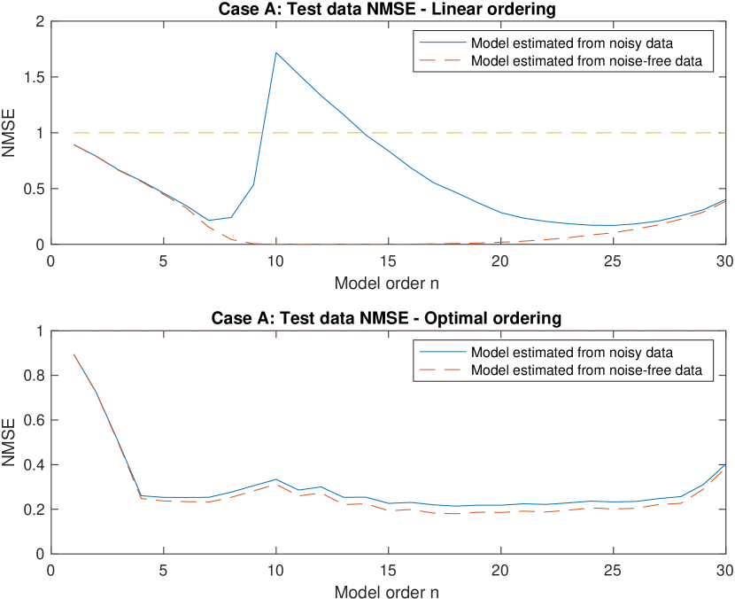
Figure 1: Case A: Graphs show normalized mean squared error as a function of model order for the linear ordering model structure (top) and the optimal ordering (bottom).

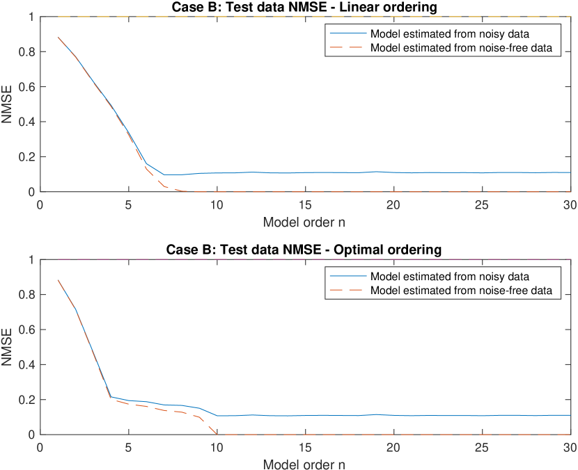
Figure 2: Case B: Graphs show normalized mean squared error as a function of model order for the linear ordering model structure (top) and the optimal ordering (bottom).

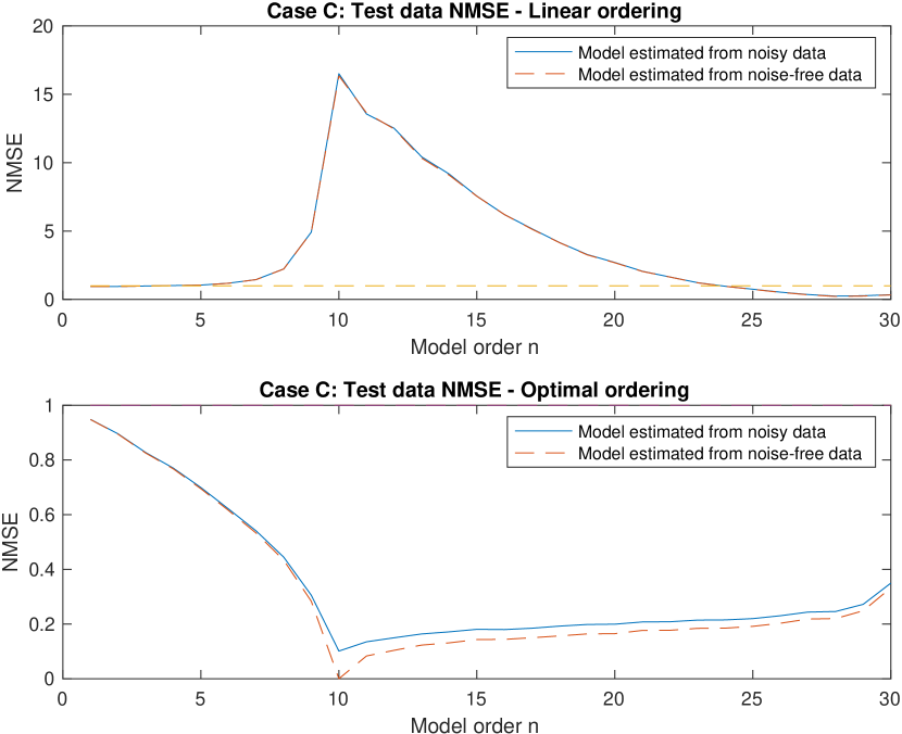
Figure 3: Case C: Graphs show normalized mean squared error as a function of model order for the linear ordering model structure (top) and the optimal ordering (bottom).

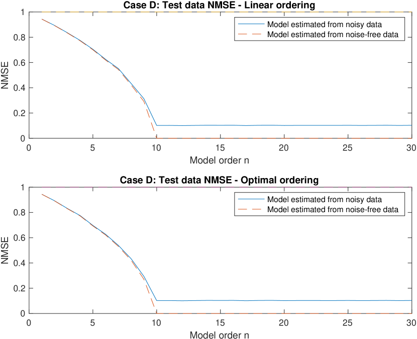
Figure 4: Case D: Graphs show normalized mean squared error as a function of model order for the linear ordering model structure (top) and the optimal ordering (bottom).

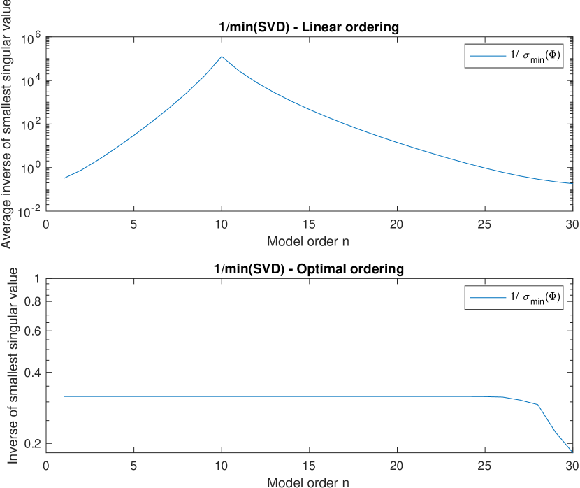
Figure 5: The graphs show the inverse of the smallest singular value for the regressor matrix $\bm{\Phi}$ as a function of model order for the linear ordering model structure (top) and the optimal ordering (bottom).

5 Conclusions

The existence of a double descent behaviour is closely related to the inverse of the smallest singular value of the associated regression matrix. A model structure with a near singular regression matrix when $n=N$ results in a double descent behavior for the NMSE on test data at other locations than the training data.

To estimate overparametrized models, i.e. more parameters than training data using the pseudo inverse solution can be resonable (NMSR$<1$) if the true parameter is close to the row space of the regression matrix. If this is not the case the solutions will have poor performance.

To obtain robust overparametrized solutions it is important to select a model class such that the minimum singular value of the associated regression matrix is as large as possible.

References

- [1] M. Belkin, D. Hsu, S. Ma, and S. Mandal, “Reconciling modern machine-learning practice and the classical bias–variance trade-off,” Proceedings of the National Academy of Sciences, vol. 116, no. 32, pp. 15 849–15 854, 2019.
- [2] G. H. Golub and C. F. Van Loan, Matrix Computations. Baltimore, Maryland: The Johns Hopkins University Press, 1989.
- [3] T. Hastie, A. Montanari, S. Rosset, and R. J. Tibshirani, “Surprises in high-dimensional ridgeless least squares interpolation,” The Annals of Statistics, vol. 50, no. 2, pp. 949–986, 2022.
- [4] R. A. Horn and C. R. Johnson, Matrix Analysis. Cambridge University Press, Cambridge, NY, 1985.
- [5] ——, Topics In Matrix Analysis. Cambridge University Press, Cambridge, NY, 1991.
- [6] A. J. Laub, Matrix Analysis for Scientists and Engineers. Siam, 2005, vol. 91.
- [7] M. Loog, T. Viering, A. Mey, J. H. Krijthe, and D. M. Tax, “A brief prehistory of double descent,” Proceedings of the National Academy of Sciences, vol. 117, no. 20, pp. 10 625–10 626, 2020.
- [8] A. H. Ribeiro, J. N. Hendriks, A. G. Wills, and T. B. Schön, “Beyond Occam’s razor in system identification: Double-descent when modeling dynamics,” IFAC-PapersOnLine, vol. 54, no. 7, pp. 97–102, 2021.
- [9] D.-F. Xia, S.-L. Xu, and F. Qi, “A proof of the arithmetic mean-geometric mean-harmonic mean inequalities,” RGMIA research report collection, vol. 2, no. 1, 1999.
- [10] C. Zhang, S. Bengio, M. Hardt, B. Recht, and O. Vinyals, “Understanding deep learning requires rethinking generalization,” 2016.