Universal platform of point-gap topological phases from topological materials

Abstract

Whereas point-gap topological phases are responsible for exceptional phenomena intrinsic to non-Hermitian systems, their realization in quantum materials is still elusive. Here we propose a simple and universal platform of point-gap topological phases constructed from Hermitian topological insulators and superconductors. We show that $(d-1)$-dimensional point-gap topological phases are realized by making a boundary in $d$-dimensional topological insulators and superconductors dissipative. A crucial observation of the proposal is that adding a decay constant to boundary modes in $d$-dimensional topological insulators and superconductors is topologically equivalent to attaching a $(d-1)$-dimensional point-gap topological phase to the boundary. We furthermore establish the proposal from the extended version of the Nielsen-Ninomiya theorem, relating dissipative gapless modes to point-gap topological numbers. From the bulk-boundary correspondence of the point-gap topological phases, the resultant point-gap topological phases exhibit exceptional boundary states or in-gap higher-order non-Hermitian skin effects.

Introduction.– There is increasing interest in the studies of non-Hermitian physics Bender (2007); Mostafazadeh and Batal (2004); Moiseyev (2011). Among them, a recent trend is the study of topology in non-Hermitian systems Ashida et al. (2020); Bergholtz et al. (2021); Okuma and Sato (2023). The prime motivation for such a research direction is that both non-Hermitian and topological systems exhibit characteristic boundary phenomena Rudner and Levitov (2009); Hu and Hughes (2011); Esaki et al. (2011); Schomerus (2013); Shen et al. (2018); Yao and Wang (2018); Kunst et al. (2018). Certain non-Hermitian systems show a boundary phenomenon called the non-Hermitian skin effect Yao and Wang (2018); Yokomizo and Murakami (2019), where a macroscopic number of bulk states are localized at the boundary. On the other hand, the bulk-boundary correspondence Hatsugai (1993), in which bulk topological invariants count the number of gapless boundary states, is one of the most notable concepts in topological systems Hasan and Kane (2010); Qi and Zhang (2011). In topological systems with the non-Hermiticity, both the non-Hermitian skin effect and the topological boundary states can coexist, and the bulk-boundary correspondence should hold in an unconventional manner Yao and Wang (2018); Kunst et al. (2018); Yao et al. (2018); Herviou et al. (2019); Song et al. (2019); Nakamura et al. (2022).

The generalization of the topological classification to non-Hermitian systems is also of interest. In the original classification of Hermitian topological insulators and superconductors Schnyder et al. (2008); Kitaev (2009); Ryu et al. (2010); Chiu et al. (2016), the gapped topology is mathematically characterized by the absence of the energy eigenstates of the Hamiltonian at the Fermi energy, $E\neq E_{\rm F}$. The natural extension to non-Hermitian systems is real line-gap topology defined by $\mathrm{Re}(E-E_{\rm F})\neq 0$ Esaki et al. (2011); Kawabata et al. (2019). Mathematically, the real line-gapped Hamiltonians are smoothly deformed into Hermitian-gapped Hamiltonians without closing the real-line gap Esaki et al. (2011); Kawabata et al. (2019); Ashida et al. (2020). Therefore, the physical consequence of the real line-gapped topology is the bulk-boundary correspondence, as in the case of the Hermitian topological phases. More generally, the line-gapped spectrum is defined as a spectrum that does not cross a specific line in the complex plane Kawabata et al. (2019). For instance, if one chooses the real axis in the complex energy plane as the reference line, such a spectrum defines the imaginary line-gap topology, which is adiabatically connected to anti-Hermitian topological phases Kawabata et al. (2019).

Remarkably, the non-Hermiticity enables another extension of topology, the point-gap topology defined by $E\neq E_{\rm P}$ Gong et al. (2018); Kawabata et al. (2019). Typically, a spectrum with nontrivial point-gap topology surrounds the reference point $E_{\rm P}$ in the complex energy plane, and thus the point-gap topology is distinct from any Hermitian-like topology. The topological classification of point-gapped Hamiltonians has been established Zhou and Lee (2019); Kawabata et al. (2019), and the physical consequences of the point-gap topological phases have been explored Gong et al. (2018); D. S. Borgnia, and A. J. Kruchkov, and R.-J. Slager (2020); N. Okuma, and M. Sato (2019); Okuma et al. (2020); Zhang et al. (2020); Okuma and Sato (2021); Kawabata et al. (2021); Yang et al. (2021); Vecsei et al. (2021); Denner et al. (2021); Hu et al. (2022); Nakamura et al. (2022); Denner et al. (2021); Lee et al. (2019a); Terrier and Kunst (2020); Bessho and Sato (2021); Lee et al. (2019b); Luo and Zhang (2019); Li et al. (2020); Okugawa et al. (2020); Kawabata et al. (2020); Fu et al. (2021); Shiozaki and Ono (2021); Palacios et al. (2021); Kim and Park (2021); Zhang et al. (2021); Ghorashi et al. (2021a, b); Zou et al. (2021); Li et al. (2022); Zhu and Gong (2022); Denner and Schindler (2023); Liu and Fulga (2023); Shang et al. (2022); Zhu and Gong (2023); Roccati et al. (2023); Nakai et al. (2023). In particular, it has been shown that the non-Hermitian skin effects originate from one-dimensional point-gap topological numbers, i.e. the spectral winding number Okuma et al. (2020); Zhang et al. (2020) or the $\mathbb{Z}_{2}$ number Okuma et al. (2020). Also, higher-dimensional point-gap topological phases may support non-Hermitian skin modes localized at topological defects, mimicking the anomaly-induced catastrophes Okuma et al. (2020); Okuma and Sato (2021); Kawabata et al. (2021); Denner and Schindler (2023); Okuma and Sato (2023). Depending on the dimension and symmetry of the system, higher-dimensional point-gap topological phases may also host boundary modes Yang et al. (2021); Vecsei et al. (2021); Denner et al. (2021); Hu et al. (2022); Nakamura et al. (2022); Denner and Schindler (2023), and one of such point-gap topological phases is called an exceptional topological insulator Denner et al. (2021). Furthermore, for the fundamental symmetry classes called AZ^† classes (see below), the correspondence between $d$-dimensional point-gap topological phases and $(d-1)$-dimensional anomalous gapless modes was suggested Lee et al. (2019a), and later proved as the extended Nielsen-Ninomiya theorem Bessho and Sato (2021).

Whereas point-gap topological phases are responsible for these exceptional phenomena intrinsic to non-Hermitian systems, their realization in quantum materials is still elusive. This paper proposes a simple and universal platform of point-gap topological phases in quantum materials. As illustrated in Fig.1, the platform consists of a $d$-dimensional topological insulator or superconductor where one of the boundaries is coupled to the environment and thus dissipative. We show that the dissipation-induced decay constant of the topological boundary modes results in a $(d-1)$-dimensional non-trivial point-gap topological number, i.e. a $(d-1)$-dimensional point-gap topological phase. We also predict exceptional boundary states or in-gap higher-order non-Hermitian skin effects based on the bulk-boundary correspondence for point-gap topological phases Denner et al. (2021); Nakamura et al. (2022).

Non-trivial topology from decay constant.– Let us start with a Chern insulator with the periodic boundary condition in the $x$-direction and the open boundary conditions at $y=1,L_{y}$ in the $y$-direction. See Fig.2 (a). The system supports a chiral edge mode at $y=1$ and an anti-chiral edge mode at $y=L_{y}$. If we couple one of the open boundaries, say $y=1$, to the environment, the chiral edge mode at $y=1$ gets the decay constant in addition to the linear spectrum,

$$h_{\rm edge}(k_{x})=vk_{x}-i\Gamma,$$ (1)

where $k_{x}$ is the momentum in the $x$-direction, $v(>0)$ is the group velocity, and $\Gamma(>0)$ is the decay constant. At first sight, the decay constant seems not to change the topology of the system, but it does change, as we see below.

To see the hidden topology due to the decay constant, we show that the complex spectrum in Eq.(1) is equivalently obtained by attaching a one-dimensional point-gap topological phase to the original Hermitian chiral edge state: The effective Hamiltonian of the attached system is

$$h_{\rm attach}(k_{x})=\left(\begin{array}[]{cc}vk_{x}&\Delta\\ \Delta^{*}&-v\sin k_{x}+i(\Gamma/2)\cos k_{x}-i(\Gamma/2)\end{array}\right),$$ (4)

where the diagonal components describe the chiral edge state and the one-dimensional point-gap topological phase, respectively, and $\Delta$ $(|\Delta|\ll 1)$ is the coupling between them. The one-dimensional point-gap topological phase is the tight-binding lattice model with asymmetric hoppings (Hatano-Nelson model Hatano and Nelson (1996, 1997, 1998)) and supports a non-zero spectral winding number. Remarkably, around $k_{x}=0$, the attached system shows the spectrum $E_{0}(k_{x})=\pm\sqrt{(vk_{x})^{2}+|\Delta|^{2}},$ and thus the original edge state has a gap in the real part of the spectrum, but there appears another chiral mode around $k_{x}=\pi$, $E_{\pi}(k_{x})=v(k_{x}-\pi)-i\Gamma.$ Therefore, by shifting the origin of the momentum space, the attached system reproduces the complex spectrum in Eq.(1). Since the attached system in Eq. (4) has a non-zero spectral winding number, the dissipative chiral edge state in Eq.(1) also should have the same non-zero winding number.

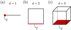
Figure 1: Universal plat forms of point-gap topological phases. $d$-dimensional topological insulators and superconductors are coupled to the environment at $x_{d}=1$.

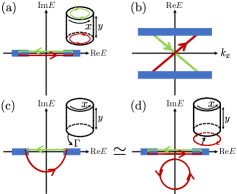
Figure 2: (a, b) Chern insulator under the periodic boundary condition in the $x$-direction and the open boundary condition in the $y$-direction. A chiral edge mode (red) at the bottom boundary and an anti-chiral edge mode (green) at the top boundary form a loop on the real axis in the complex energy plane. (c) Chern insulator (a) with the decay constant term $\Gamma$ at the bottom boundary. (d) Chern insulator (a) attached the Hatano-Nelson model at the bottom boundary.

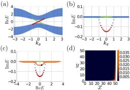
Figure 3: The QWZ model ($m=-1.5$, $L_{x}=L_{y}=50$) in Eq.(5) with $-i\Gamma\sigma_{0}$ term ($\Gamma=0.2$) at the $y=1$ boundary. (a, b) The real and imaginary parts of the spectrum under the periodic boundary condition in the $x$-direction. (c) Comparison of the complex energy spectra under the open boundary condition (orange) and the periodic boundary condition (other colors) in the $x$-direction. (d) The skin mode with the energy $E=0.30-0.04i$ (the star symbol in (c)).

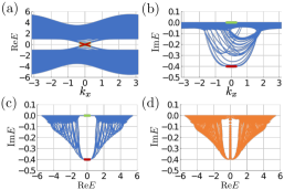
Figure 4: 3D chiral symmetric topological insulator ($L_{x}=300$, $L_{y}=L_{z}=20$) in Eq.(7) with $-i\Gamma\sigma_{0}\tau_{0}$ ($\Gamma=0.2$) term at the $z=1$ boundary. (a,b,c) The real and imaginary parts of the spectrum under the periodic boundary conditions in the $x$ and $y$-directions. (d) The complex spectrum under the periodic boundary condition in the $x$-direction and the open boundary condition in the $y$-direction. There appear in-gap boundary modes.

Whereas the above argument is rather heuristic, we also have a convincing discussion on the non-trivial topology: For a rigorous discussion, we assume that the decay constant induced on the boundary is uniform and thus retains the lattice translation symmetry along the edge (namely the $x$-direction) . Then, from the Bloch theorem, any energy eigenstate in the present model should be labeled by $k_{x}$, and we have the $2\pi$-periodicity in $k_{x}$ for the energy eigenstates. This means that the chiral edge state at $y=1$ and the anti-chiral edge one at $y=L_{y}$ should be exchanged when changing $k_{x}$ by $2\pi$ since they cannot go back to themself after the one-period. As a result, they make a loop in the complex energy plane, as illustrated in Fig.2. In the absence of dissipation, the loop sticks to the real axis of the complex energy plane, as in Fig.2 (a), which implies that the spectral winding number is zero. However, once the chiral edge mode at $y=1$ has the imaginary part of the energy due to dissipation, the loop is extended to the imaginary energy direction so it immediately gets a non-zero spectral winding number as shown in Fig.2 (c). Therefore, the decay constant of the chiral edge mode results in the non-trivial point-gap topology. We can also confirm that the decay of the chiral edge mode is topologically the same as the attachment of the one-dimensional Hatano-Nelson model to the boundary: The Hatano-Nelson model gives a loop spectrum in the complex energy plane in Fig.2 (d). Then through the reconnection of the spectra between the Hatano-Nelson model and the chiral edge mode, we smoothly obtain the complex spectrum in Fig.2 (c) .

We can make a concrete prediction due to the non-trivial spectral winding number from the decay constant. Namely, the system exhibits the non-Hermitian skin effect under the open boundary condition in the $x$-direction. To check the prediction, we consider the Chern insulator modeled by Qi, Wu, and Zhang (QWZ) Qi et al. (2006)

$$H_{\rm QWZ}({\bm{k}}) =\sin k_{x}\sigma_{x}+\sin k_{y}\sigma_{y}$$

$$+(m+\cos k_{x}+\cos k_{y})\sigma_{z},$$ (5)

which has the Chern number 1 for $-2<m<0$. Here $\sigma_{\mu=0,x,y,z}$ are the Pauli matrices. When we impose the open boundary condition on the $y$-direction and put the imaginary onsite potential $-i\Gamma\sigma_{0}$ along the boundary at $y=1$, the chiral edge state gets a finite lifetime, as shown in Figs. 3(a) and 3(b). Then, if we further impose the open boundary condition on the $x$-direction, the system shows the non-Hermitian skin effect. See Fig.3(c). We have $O(L)$ corner skin modes shown in Fig.3(d). This behavior entirely agrees with the prediction .

Universal platform of point-gap topological phases.– So far, we have considered a two-dimensional Chern insulator and have shown how to realize a one-dimensional point-gap topological phase from the Chern insulator. Now we generalize the idea to other topological insulators and superconductors. Let us consider a $d$-dimensional topological insulator or superconductor. Under the open boundary conditions at $x_{d}=1,L_{d}$ in the $x_{d}$-direction, we have topological gapless boundary modes with an opposite topological charge at opposite boundaries. Then, if we couple one of the boundaries, say $x_{d}=1$, to the environment, the topological gapless modes at $x_{d}=1$ get a finite lifetime, namely the imaginary part of the spectrum, due to dissipation. As we will see shortly, this configuration realizes a $(d-1)$-dimensional point-gap topological phase.

To prove the above statement, we first clarify the symmetry of the system. The fundamental onsite symmetries for topological insulators and superconductors are time-reversal (TRS), particle-hole (PHS), and their combination, chiral symmetry (CS). These Altland-Zirnbauer (AZ) symmetries Altland and Zirnbauer (1997) protect topological gapless boundary modes of topological insulators and superconductors Schnyder et al. (2008); Kitaev (2009); Ryu et al. (2010); Chiu et al. (2016). In the presence of the coupling to the environment, however, we cannot retain these symmetries in their original form. Causal fermionic theories require other onsite symmetries intrinsic to non-Hermitian systems Lieu et al. (2020); Yoshida et al. (2020), which we call AZ^† symmetries Kawabata et al. (2019). The AZ^† symmetries consist of TRS^†: $H=U_{T}H^{T}U_{T}^{\dagger}$, $U_{T}U_{T}^{*}=\pm 1$, PHS^†: $H=-U_{C}H^{*}U_{C}^{\dagger}$, $U_{C}U_{C}^{*}=\pm 1$, CS^†: $H=-U_{\Gamma}H^{\dagger}U_{\Gamma}^{\dagger}$, $U_{\Gamma}U_{\Gamma}=1$, where $H$ is the Hamiltonian, and $U_{T}$, $U_{C}$ and $U_{\Gamma}$ are unitary matrices Kawabata et al. (2019). For a Hermitian $H$, the AZ^† symmetries coincide with the original AZ symmetries. The presence and absence of the AZ^† symmetries define the ten-fold AZ^† classes Kawabata et al. (2019). See Table 1. One can easily check that the onsite decay constant term $-i\Gamma{\bm{1}}$ due to dissipation respects the AZ^† symmetries .

A critical mathematical result for our theory is the extended Nielsen-Ninomiya theorem Bessho and Sato (2021), which holds for systems in the AZ^† classes. The theorem relates the bulk gapless points at the energies $E_{\alpha}$ with the topological charges $\nu_{\alpha}$ to the point-gap topological number $n$ at the reference energy $E_{\rm P}$,

$$n(E_{\rm P})=\sum_{{\rm Im}(E_{\alpha}-E_{\rm P})>0}\nu_{\alpha}=-\sum_{{\rm Im}(E_{\alpha}-E_{\rm P})<0}\nu_{\alpha},$$ (6)

where the index $\alpha$ labels the gapless bulk states. This theorem implies that if topological gapless states have different lifetimes, there exists a region of $E_{\rm P}$ where $n$ is non-zero, namely we have a point-gap topological phase characterized by $n$.

Now we come back to our system, i.e. a $d$-dimensional topological insulator or superconductor with the open boundary condition in the $x_{d}$-direction. Our system belongs to an AZ^† symmetry class when the system is coupled to the environment at $x_{d}=1$. Regarding the site index in the $x_{d}$-direction as an internal degree of freedom, we can identify the system as a $(d-1)$ dimensional system with ”bulk” gapless states with the internal index $x_{d}=1,L_{d}$. Then, by the coupling to the environment at $x_{d}=1$, the $(d-1)$-dimensional bulk gapless states at $x_{d}=1$ have a different decay constant than those at $x_{d}=L_{d}$. Therefore, from the extended Nielsen-Ninomiya theorem in Eq.(6), there exists a region of $E_{\rm P}$ where the $(d-1)$-dimensional point-gap topological number $n$ becomes non-zero. The non-zero value of $n$ is given by the $d$-dimensional bulk topological number of the original topological insulator/superconductor since the total topological charge of the gapless states at $x_{d}=1$ coincides with it up to sign.

Table 1: Point-gap topological table for insulators and superconductors with dissipation at $x_{d}=1$. Here $\delta=(d-1)-D$, where $d$ is the spatial dimension of the topological insulators and superconductors and $D$ is the dimension of a sphere surrounding a topological defect. The topological defect goes through the $x_{d}$-direction. The superscripts SE and BS indicate the topological numbers predicting non-Hermitian skin effects and boundary states, respectively. See also Ref.Nakamura et al. (2022). For $D=0$, this table reproduces that for $(d-1)$-dimensional point-gap phases in AZ^† classes in Kawabata et al. (2019).

AZ† class	TRS†	PHS†	CS	$\delta=0$	$\delta=1$	$\delta=2$
A	$0$	$0$	$0$	$0$	$\mathbb{Z}^{\rm SE}$	$0$
AIII	$0$	$0$	$1$	$\mathbb{Z}$	$0$	$\mathbb{Z}^{\rm BS}$
$\text{AI}^{{\dagger}}$	$+1$	$0$	$0$	$0$	$0$	$0$
$\text{BDI}^{{\dagger}}$	$+1$	$+1$	$1$	$\mathbb{Z}$	$0$	$0$
$\text{D}^{{\dagger}}$	$0$	$+1$	$0$	$\mathbb{Z}_{2}$	$\mathbb{Z}^{\rm SE}$	$0$
$\text{DIII}^{{\dagger}}$	$-1$	$+1$	$1$	$\mathbb{Z}_{2}$	$\mathbb{Z}_{2}^{\rm SE}$	$(2\mathbb{Z}+1)^{\rm SE}$
						$2\mathbb{Z}^{\rm BS}$
$\text{AII}^{{\dagger}}$	$-1$	$0$	$0$	$0$	$\mathbb{Z}_{2}^{\rm SE}$	$\mathbb{Z}_{2}^{\rm SE}$
$\text{CII}^{{\dagger}}$	$-1$	$-1$	$1$	2$\mathbb{Z}$	$0$	$\mathbb{Z}_{2}^{\rm BS}$
$\text{C}^{{\dagger}}$	$0$	$-1$	$0$	$0$	$2\mathbb{Z}^{\rm SE}$	$0$
$\text{CI}^{{\dagger}}$	$+1$	$-1$	$1$	$0$	$0$	$2\mathbb{Z}^{\rm BS}$

Predictions.– The non-zero $(d-1)$-dimensional point-gap topological number $n$ gives rise to several consequences in the physical properties of the system. First, it predicts the appearance of $(d-2)$-dimensional boundary modes or skin modes when imposing the additional open boundary condition on a different direction than $x_{d}$, say the $x_{d-1}$-direction Nakamura et al. (2022). For $d=2$, the non-zero $n$ predicts a second-order non-Hermitian skin effect like the Chern insulator case in Fig.3. The second-order skin modes form a generalized Kramers pair Sato et al. (2012); Kawabata et al. (2019) when the original system has fermionic time-reversal symmetry. For $d=3$, an odd $n$ in class DIII^† (time-reversal invariant topological superconductor) and a non-trivial $n$ in class AII^† (topological insulator) imply the in-gap non-Hermitian skin effects. Still, other non-zero $n$s’ predict boundary modes. (See Table 1 with $D=0$ introduced below.)

Second, the proposed system also may have similar localized modes in the presence of topological defects. The topological defects should go through the $x_{d}$-direction since our theory treats the site index in the $x_{d}$-direction as an internal degree of freedom. Then, we can obtain the point-gap topological table in the presence of such topological defects by generalizing the argument by Teo and Kane Teo and Kane (2010) to point-gap topological phases. See Table 1. In the new table, the space dimension $d-1$ of the point-gap topological phases is replaced by $\delta=(d-1)-D$ $(\geq 0)$, where $D$ $(\leq d-1)$ is the dimension of a sphere surrounding the topological defect. In particular, if we insert the $\pi$-flux ($D=1$) in the $x_{3}$-direction through a three-dimensional time-reversal invariant superconductor with an odd number of the three-dimensional winding number or a three-dimensional time-reversal invariant topological insulator, we have a non-trivial $\mathbb{Z}_{2}^{\rm SE}$ number for class DIII^† or class AII^† with $\delta=1$, in the presence of dissipation at $z=1$. Thus, we obtain the non-Hermitian skin modes localized on the $\pi$-flux.

Finally, the point-gap topology also stabilizes the original topological boundary modes of the topological insulator/superconductor. In general, the topological boundary modes of the topological insulator/superconductor have tiny gaps because of the mixing with those at an opposite boundary. Therefore, for finite $L_{d}$, they are not always gapless and do not have well-defined topological charges in a mathematically rigorous sense. In contrast, when the point-gap topological number $n$ becomes non-trivial, the extended Nielsen-Ninomiya theorem in Eq.(6) ensures the well-defined topological charges $\nu_{\alpha}$, which implies that the mixing disappear and the tiny gaps close. Indeed, the gapless modes at $x_{d}=1$ and those at $x_{d}=L_{d}$ have different imaginary parts of the energy, and thus they do not mix. The gap closing of the boundary modes should be observed in high-resolution spectrum-sensitive experiments and sharpens the topological phenomena of the boundary modes.

Examples.– We check the validity of our scheme in various topological materials. For $d=1$, the dissipation effect for a superconducting nanowire has been discussed in literature Pikulin and Nazarov (2013); San-Jose et al. (2016); Avila et al. (2019); Okuma and Sato (2021); Liu et al. (2022). The coupling of a Majorana end state to the environment is shown to give a non-trivial zero-dimensional point-gap $\mathbb{Z}_{2}$ number Okuma and Sato (2021). It has been also demonstrated that the dissipation stabilizes the Majorana end state Liu et al. (2022). For $d=2$, we have already shown above that our theory for a Chern insulator gives the second-order non-Hermitian skin effect. For $d=3$, exactly the same scheme was discussed for a three-dimensional time-reversal invariant topological insulator Okuma and Sato (2023), which showed that non-Hermitian skin modes appear in the $\pi$-flux. (See Fig. 5b in Ref.Okuma and Sato (2023).) In Fig.4, we also show the result for the three-dimensional chiral symmetric topological insulator,

$$H_{\rm CSTI}({\bm{k}}) =[\sin k_{x}+(1-\cos k_{y})]\sigma_{x}\tau_{x}+\sin k_{y}\sigma_{y}\tau_{x}$$

$$+\sin k_{z}\sigma_{z}\tau_{x}+(-2+\sum_{i=x,y,z}\cos k_{i})\sigma_{0}\tau_{y},$$ (7)

where $\sigma_{\mu}$ and $\tau_{\mu}$ are the Pauli matrices, CS is $U_{\Gamma}=\sigma_{0}\tau_{z}$ and the onsite dissipation term $-i\Gamma\sigma_{0}\tau_{0}$ is placed at $z=1$. The system realizes the $\delta=2$ ($d=3$, $D=0$) AIII class with $\mathbb{Z}^{\rm BS}=1$. Under the open boundary conditions in both $z$ and $y$-directions, the system hosts a boundary state inside the point gap, as expected .

Summary.– We propose a universal platform for point-gap topological phases constructed from topological insulators and superconductors. Using various independent arguments, we establish that dissipation on a boundary of $d$-dimensional topological materials results in $(d-1)$-dimensional point-gap topological phases. We also confirm the validity of our proposal for various topological materials.

Our scheme applies to any topological materials in the original topological periodic table Schnyder et al. (2008); Kitaev (2009); Ryu et al. (2010); Chiu et al. (2016). For instance, by connecting a metal to an edge of a quantum Hall state in graphene, we can realize a point-gap topological phase similar to Fig.3. The resulting non-Hermitian skin effect can be observed as the chiral tunneling effect Yi and Yang (2020). Another candidate is a topological superconducting nanowire with a Zeeman field Sato and Ando (2017). By coupling a lead to one of the ends of the nanowire, the system displays a point-gap topological phase in 0D class D^†. We can also use the topological insulator Bi₂Se₃ and the variants Ando (2013) to similarly realize a point-gap topological phase in 2D class AII^†.

Note added: A part of the present work was reported in Inaka et al. . We are aware of related works Ma et al. (2023); Schindler et al. (2023) after the completion of this work.

Acknowledgments.– This work was supported by JST CREST Grant No. JPMJCR19T2 and KAKENHI Grant No. JP20H00131. D.N. was supported by JST, the establishment of university fellowships towards the creation of science technology innovation, Grant Number JPMJFS2123. N.O. was supported by JSPS KAKENHI Grant No. JP20K14373.

Supplemental Material

S1 S1. Skin modes versus in-gap boundary modes

Here we clarify the difference between skin modes and in-gap boundary modes. As discussed in Okuma and Sato (2023); Nakai et al. (2023), the right and left eigenstates for a skin mode should be localized in opposite boundaries, while those for an in-gap boundary mode are localized in the same boundary.

Figure S1 depicts the density profile of a corner skin mode in Fig.3 (d). As mentioned above, the right and left eigenstates of the corner skin mode are localized at different corners. In Fig.S1 (b), we impose the biorthogonal normalization on the corner skin mode where the inner product between the right and left eigenstate is 1. Because the right and left eigenstates rarely overlap, the amplitude of the left eigenstate becomes large. (Here the inner product of the right eigenstate is normalized as 1.)

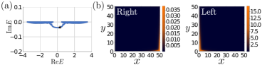
Figure S1: The QWZ model ($m=-1.5$, $L_{x}=L_{y}=50$) in Eq.(3) with $-i\Gamma\sigma_{0}$ term ($\Gamma=0.2$) at the $y=1$ boundary. (a) The complex spectrum under the open boundary condition in the $x$-direction. (b) The density profile of the right and left eigenstates for a corner skin mode with the energy $E=0.30-0.04i$ (the star symbol in (a)).

In contrast, the in-gap boundary modes in Fig.4 exhibit different behaviors. As illustrated in Figs.S2 (d) and (e), the right and left eigenstates of the in-gap boundary modes in Fig.4 are localized at the same corner. Note that the three-dimensional chiral symmetric topological insulator $H_{\rm CSTI}({\bm{k}})$ in Eq.(5) has an additional mirror reflection symmetry,

$$M_{y}H_{\rm CSTI}({\bm{k}})M_{y}^{\dagger}=H(k_{x},-k_{y},k_{z}),\quad M_{y}=\sigma_{y}\tau_{y}.$$ (S1)

This symmetry preserves even when we impose the open boundary condition in the $z$-direction and place the on-site dissipation term $-i\Gamma\sigma_{0}\tau_{0}$ on the boundary at $z=1$. Because of this additional symmetry, the in-gap boundary modes have two-fold degeneracy.

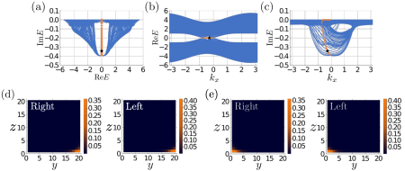
Figure S2: 3D chiral symmetric topological insulator ($L_{x}=300$, $L_{y}=L_{z}=20$) in Eq.(5) with $-i\Gamma\sigma_{0}\tau_{0}$ ($\Gamma=0.2$) term at the $z=1$ boundary. (a,b,c) Complex spectrum of the system under the periodic boundary conditions in the $x$-direction and the open boundary condition in the $y$-directions. The orange curves indicate the in-gap boundary states. The in-gap boundary states are doubly degenerate because of mirror reflection symmetry in Eq.(S1). (d) The density profile of the right and left eigenstates for an in-gap boundary state with the energy $E=-0.34i$. (the star symbols in (a,b,c)). (e) The density profile of the right and left eigenstates for the mirror symmetry partner of the in-gap boundary state in (d).

S2 S2. Derivation of Dissipation term

In this section, we microscopically derive the dissipation term used in the main text. As we shall show below, if we couple a good metal, whose bandwidth is much larger than that of the topological material, to the topological material, then we naturally obtain the constant dissipation term. (See Eq.(S27).)

Let us consider a $d$ dimensional topological insulator described by the lattice Hamiltonian

$$\hat{H}_{\rm top}=\sum_{ij}a^{\dagger}_{i}(H_{\rm top})_{ij}a_{j},$$ (S2)

where $i$ is the index labeling the lattice site and other internal degrees of freedom such as spin and orbital, and $a_{i}$ and $a_{i}^{\dagger}$ are fermionic annihilation and creation operators. As in the main text, we assume the open boundary condition in the $x_{d}$ direction and the periodic boundary conditions in the other directions. Then, as an environment, we couple a metal described by the lattice Hamiltonian

$$\hat{H}_{\rm env}=\sum_{ij}b^{\dagger}_{i}(H_{\rm env})_{ij}b_{j}$$ (S3)

to the topological insulator at the bottom ($x_{d}=L$) with the coupling term

$$\hat{H}_{\rm coupling}=\sum_{ij}a^{\dagger}_{i}(\tau)_{ij}b_{j}+{\rm h.c.},$$ (S4)

where $b_{i}$ and $b_{i}^{\dagger}$ are fermionic annihilation and creation operators. The total Hamiltonian is $\hat{H}=\hat{H}_{\rm top}+\hat{H}_{\rm env}+\hat{H}_{\rm coipling}$, which is rewritten in the following simple form:

$$\hat{H}=\sum_{\alpha i,\beta j}c^{\dagger}_{\alpha i}(H)_{\alpha i,\beta j}c_{\beta j}$$ (S5)

where $\alpha=1,2$ is the index distinguishing the topological insulator and the environment metal with $c_{1i}=a_{i}$, $c_{2i}=b_{i}$, $c^{\dagger}_{1i}=a^{\dagger}_{i}$, $c^{\dagger}_{2i}=b^{\dagger}_{i}$, and $H_{\alpha i,\beta j}$ is the matrix Hamiltonian given by

$$H_{\alpha i,\beta j}=\left(\begin{array}[]{cc}(H_{\rm top})_{ij}&(\tau)_{ij}\\ (\tau*)_{ji}&(H_{\rm env})_{ij}\end{array}\right).$$ (S8)

The Hamiltonians $\hat{H}_{\rm top}$ and $\hat{H}_{\rm env}$ are Hermitian and so is the total Hamiltonian $\hat{H}$.

To derive the effective Hamiltonian, we employ the retarded Green function defined by

$$G^{\rm R}_{\alpha i,\beta j}(t)=-i\theta(t)\langle c_{\alpha i}(t)c_{\beta j}^{\dagger}+c^{\dagger}_{\beta j}c_{\alpha i}(t)\rangle,$$ (S9)

where $c_{\alpha i}(t)=e^{i\hat{H}t}c_{\alpha i}e^{-i\hat{H}t}$ and $\langle\cdots\rangle={\rm tr}(e^{-\beta\hat{H}}\cdots)/{\rm tr}(e^{-\beta\hat{H}})$. Using the Heisenberg equation $i\partial_{t}c_{\alpha i}(t)=\sum_{\beta j}H_{\alpha i,\beta,j}c_{\beta j}$, we have

$$\left(\begin{array}[]{cc}E+i\eta-H_{\rm top}&-\tau\\ -\tau^{\dagger}&E+i\eta-H_{\rm env}\end{array}\right)\left(\begin{array}[]{cc}G^{\rm R}_{\rm top}&G^{\rm R}_{\rm te}\\ G^{\rm R}_{\rm et}&G^{\rm R}_{\rm env}\end{array}\right)=1,$$ (S14)

where $G^{\rm R}_{1i,1j}=(G^{\rm R}_{\rm top})_{ij}$, $G^{\rm R}_{1i,2j}=(G^{\rm R}_{\rm te})_{ij}$, $G^{\rm R}_{2i,1j}=(G^{\rm R}_{\rm et})_{ij}$ and $G^{\rm R}_{2i,2j}=(G^{\rm R}_{\rm env})_{ij}$. Here and below, the index $i$ is often implicit. This equation leads to

$$(E+i\eta-H_{\rm top})G^{\rm R}_{\rm top}-\tau G^{\rm R}_{\rm et}=1,$$

$$(E+i\eta-H_{\rm env})G^{\rm R}_{\rm et}-\tau^{\dagger}G^{\rm R}_{\rm top}=0,$$ (S15)

then, introducing the retarded Green function $g_{\rm env}$ of the environment as

$$g_{\rm env}^{-1}=(E+i\eta-H_{\rm env}),$$ (S16)

we obtain

$$G^{\rm R}_{\rm et}=g_{\rm env}\tau^{\dagger}G^{\rm R}_{\rm top}.$$ (S17)

from the second equation in Eq. (S15). Then, the first equation in Eq.(S15) yields

$$(E+i\eta-H_{\rm top}-\tau g_{\rm env}\tau^{\dagger})G^{\rm R}_{\rm top}=1,$$ (S18)

which implies that the topological insulator coupled to the environment has the effective Hamiltonian Datta (1995)

$$H_{\rm eff}=H_{\rm top}+\tau g_{\rm env}\tau^{\dagger}.$$ (S19)

As we show immediately, the second term of the effective Hamiltonian is non-Hermitian and provides the dissipation term in the main text.

To evaluate the second term of Eq.(S19), we assume a simple form of the coupling $\tau$,

$$\tau_{ij}=\tau_{\rm c}\delta_{i_{\perp},L_{d}}\delta_{j_{\perp},L_{d}+1}\delta_{{\bm{i}}_{\parallel},{\bm{j}}_{\parallel}}\delta_{\sigma\sigma^{\prime}},$$ (S20)

with a complex number $\tau_{c}$. Here we explicitly write down the lattice site $(\vec{i}_{\parallel},i_{\perp})$ and the internal degrees of freedom $\sigma$ in the indices $i=({\bm{i}}_{\parallel},i_{\perp},\sigma)$ and $j=({\bm{j}}_{\parallel},j_{\perp},\sigma^{\prime})$, and $i_{\perp}=L_{d}$ indicates the bottom boundary of the topological material. (The topological material extends between $i_{\perp}=1$ and $i_{\perp}=L_{d}$, and the metal does at $i_{\perp}\geq L_{d}+1$.) This coupling leads to

$$(\tau g_{\rm env}\tau^{\dagger})_{ij}=\left\{\begin{array}[]{cl}|\tau_{\rm c}|^{2}(g_{\rm env})_{({\bm{i}}_{\parallel},L_{d}+1,\sigma)({\bm{j}}_{\parallel},L_{d}+1,\sigma^{\prime})},&\mbox{for $i_{\perp}=j_{\perp}=L_{d}$}\\ 0,&\mbox{others}\end{array}\right.,$$ (S23)

and thus, the second term is non-zero only at the bottom boundary of the topological material. For further evaluation, we use the lattice translation symmetry along the boundary, which enables the following momentum representation of $g_{\rm env}$,

$$(g_{\rm env})_{({\bm{i}}_{\parallel},L_{d}+1,\sigma)({\bm{j}}_{\parallel},L_{d}+1,\sigma^{\prime})}=\frac{1}{V_{d-1}}\sum_{{\bm{k}}_{\parallel}}g_{\rm env}({\bm{k}}_{\parallel},L_{d}+1)\delta_{\sigma,\sigma^{\prime}}e^{i{\bm{k}}_{\parallel}({\bm{i}}_{\parallel}-{\bm{j}}_{\parallel})},$$ (S24)

where we assume that the metal Hamiltonian $H_{\rm emv}$ is independent of $\sigma$ for simplicity, and $V_{d-1}$ is the volume of the $(d-1)$-dimensional boundary. If we further assume that the metal is symmetric concerning the $\pi$-rotation normal to the boundary, we find that the imaginary part of $(\tau g_{\rm env}\tau^{\dagger})_{ij}$ with $i_{\perp}=j_{\perp}=L_{d}$ is given by

$${\rm Im}(\tau g_{\rm env}\tau^{\dagger})_{ij} =\frac{|\tau_{c}|^{2}}{V_{d-1}}\sum_{{\bm{k}}_{\parallel}}{\rm Im}\left[g_{\rm env}({\bm{k}}_{\parallel},L_{d}+1)\right]\delta_{\sigma,\sigma^{\prime}}e^{i{\bm{k}}_{\parallel}({\bm{i}}_{\parallel}-{\bm{j}}_{\parallel})}.$$

$$=-\frac{|\tau_{c}|^{2}}{\pi V_{d-1}}\sum_{{\bm{k}}_{\parallel}}\rho_{\rm env}({\bm{k}}_{\parallel},E)e^{i{\bm{k}}_{\parallel}({\bm{i}}_{\parallel}-{\bm{j}}_{\parallel})},$$ (S25)

where $\rho_{\rm env}({\bm{k}}_{\parallel},E)$ is the density of states of the metal with parallel momentum ${\bm{k}}_{\parallel}$ and energy $E$ at the boundary $i_{\parallel}=L_{d}+1$. Here we have used the Green function representation of the density of states:

$$\rho_{\rm env}({\bm{k}}_{\parallel},E)=-\pi{\rm Im}\left[g_{\rm env}({\bm{k}}_{\parallel},L_{d}+1)\right].$$ (S26)

For a good metal of which the bandwidth is much larger than that of the topological insulator, we can approximate the density of state by the constant averaged value $\bar{\rho}_{\rm env}$ Aoki et al. (2014), then we obtain

$${\rm Im}(\tau g_{\rm env}\tau^{\dagger})_{ij}=-\frac{|\tau_{c}|^{2}}{\pi}\bar{\rho}_{\rm env}\delta_{{\bm{i}}_{\parallel},{\bm{j}}_{\parallel}}\delta_{i_{\perp},L_{d}}\delta_{j_{\perp},L_{d}}\delta_{\sigma,\sigma^{\prime}},$$ (S27)

which provide the dissipation term $-i\Gamma$ with $\Gamma=|\tau_{c}|^{2}\bar{\rho}_{\rm env}/\pi$ at the bottom boundary of the topological insulator. Note that ${\rm Re}[g_{\rm env}({\bm{k}}_{\parallel},L_{d}+1)]$ only renormalize $H_{\rm top}$ at the boundary, and can be ignored if the bulk gap of the topological insulator is large enough.

If we consider a topological superconductor instead of a topological insulator, the Hamiltonian in Eq.(S2) is modified as

$$\hat{H}_{\rm top}=\sum_{ij}a^{\dagger}_{i}(H_{\rm normal})_{ij}a_{j}+\frac{1}{2}\sum_{ij}\left[a_{i}^{\dagger}(\Delta)_{ij}a^{\dagger}_{j}+{\rm h.c}\right].$$ (S28)

Still, we can derive the dissipation term in a similar manner by using the Green function in Nambu space. From a parallel argument, we have the dissipation term at the boundary

$$\begin{pmatrix}-i\Gamma\delta_{{\bm{i}}_{\parallel},{\bm{j}}_{\parallel}}\delta_{i_{\perp},L_{d}}\delta_{j_{\perp},L_{d}}\delta_{\sigma,\sigma^{\prime}}&0\\ 0&-i\Gamma\delta_{{\bm{i}}_{\parallel},{\bm{j}}_{\parallel}}\delta_{i_{\perp},L_{d}}\delta_{j_{\perp},L_{d}}\delta_{\sigma,\sigma^{\prime}}\end{pmatrix},$$ (S29)

with $\Gamma=|\tau_{c}|^{2}\bar{\rho}_{\rm env}/\pi$ in the Nambu space representaion.

S3 S3. AZ^† symmetry

In this section, we show that AZ symmetry in the total Hamiltonian results in AZ^† symmetry in the effective Hamiltonian in Sec. S2.

First, we introduce AZ symmetry in terms of fermionic operators. The AZ symmetry is local symmetry consisting of TRS, PHS, and CS defined by

$$\mbox{TRS}:\quad \hat{T}c^{\dagger}_{\alpha i}\hat{T}^{-1}=\sum_{j}c^{\dagger}_{\alpha j}(U^{\alpha}_{T})_{ji},\quad\hat{T}c_{\alpha i}\hat{T}^{-1}=\sum_{j}c_{\alpha j}(U^{\alpha}_{T})^{*}_{ji},$$ (S30)

$$\mbox{PHS}:\quad \hat{C}c^{\dagger}_{\alpha i}\hat{C}^{-1}=\sum_{j}c_{\alpha j}(U^{\alpha}_{C})^{*}_{ji},\quad\hat{C}c_{\alpha i}\hat{C}^{-1}=\sum_{j}c^{\dagger}_{\alpha j}(U^{\alpha}_{C})_{ji},$$ (S31)

$$\mbox{CS}:\quad \hat{\Sigma}c^{\dagger}_{\alpha i}\hat{\Sigma}^{-1}=\sum_{j}c_{\alpha j}(\Gamma^{\alpha})^{*}_{ji},\quad\hat{\Sigma}c_{\alpha i}\hat{\Sigma}^{-1}=\sum_{j}c^{\dagger}_{\alpha j}(\Gamma^{\alpha})_{ji},$$ (S32)

where $\alpha$ is the label distinguishing the topological material ($\alpha=1$) and the environment metal ($\alpha=2$), $\hat{T}$ and $\hat{\Sigma}$ are anti-unitary operators, $\hat{C}$ is a unitary operator, and $U^{\alpha}_{T}$, $U^{\alpha}_{C}$, and $\Gamma^{\alpha}$ are unitary matrices. In the absence of PHS, $c_{\alpha i}$ is the electron operator ($c_{1i}=a_{i}$ and $c_{2i}=b_{i}$), but in the presence of PHS, it represents the corresponding Nambu spinor. Since AZ symmetry is local symmetry, it does not mix different $\alpha$.

For the quadratic Hamiltonian

$$\hat{H}=\sum_{\alpha i,\beta j}c^{\dagger}_{\alpha i}(H)_{\alpha i,\beta j}c_{\beta j},$$ (S33)

the above operations reproduce the standard AZ symmetry:

$$\mbox{TRS}:\quad [\hat{H},\hat{T}]=0\quad\Leftrightarrow\quad(U_{T}^{\alpha})_{ip}(H)^{*}_{\alpha p,\beta q}(U_{T}^{\beta\dagger})_{qj}=(H)_{\alpha i,\beta j},$$ (S34)

$$\mbox{PHS}:\quad [\hat{H},\hat{C}]=0\quad\Leftrightarrow\quad(U_{C}^{\alpha})_{ip}(H^{T})_{\alpha p,\beta q}(U_{C}^{\beta\dagger})_{qj}=-(H)_{\alpha i,\beta j},$$ (S35)

$$\mbox{CS}:\quad [\hat{H},\hat{\Sigma}]=0\quad\Leftrightarrow\quad(\Gamma^{\alpha})_{ip}(H^{\dagger})_{\alpha p,\beta q}(\Gamma^{\beta\dagger})_{qj}=-(H)_{\alpha i,\beta j},\quad{\rm tr}H^{*}=0.$$ (S36)

Note that one can omit ${\rm tr}H^{*}=0$ in Eq.(S36) if $\hat{H}$ is Hermitian as one can derive it from the first equation in the right-hand side of Eq.(S36).

To examine AZ symmetry in the effective Hamiltonian, let us consider the retarded Green function for the topological material Yoshida et al. (2020):

$$(G^{\rm R}_{\rm top})_{ij}=-i\theta(t)\langle a_{i}(t)a^{\dagger}_{j}+a^{\dagger}_{j}a_{i}(t)\rangle.$$ (S37)

First, we examine TRS in the effective Hamiltonian. When $\hat{H}$ has TRS, i.e. $\hat{T}^{-1}\hat{H}\hat{T}=\hat{H}$, we have

$$\langle a_{i}(t)a^{\dagger}_{j}\rangle ={\rm tr}(e^{-\beta\hat{T}^{-1}\hat{H}\hat{T}}e^{i\hat{T}^{-1}\hat{H}\hat{T}t}a_{i}e^{-i\hat{T}^{-1}\hat{H}\hat{T}t}a^{\dagger}_{j})/{\rm tr}(e^{\beta\hat{H}})$$

$$={\rm tr}(\hat{T}^{-1}e^{-\beta\hat{H}}e^{-i\hat{H}t}\hat{T}a_{i}\hat{T}^{-1}e^{i\hat{H}t}\hat{T}a^{\dagger}_{j}\hat{T}^{-1}\hat{T}).$$ (S38)

Since $\hat{T}$ is anti-unitary, we have

$$\langle n|\hat{T}^{-1}\hat{O}|m\rangle =(\langle\hat{T}n|\hat{T}\hat{T}^{-1}\hat{O}|m\rangle)^{*}$$

$$=(\langle\hat{T}n|\hat{T}\hat{T}^{-1}\hat{O}\hat{T}^{-1}\hat{T}|m\rangle)^{*}$$

$$=(\langle\hat{T}n|\hat{O}\hat{T}^{-1}|\hat{T}m\rangle)^{*},$$ (S39)

which leads to ${\rm tr}(\hat{T}^{-1}\hat{O})={\rm tr}(\hat{O}\hat{T}^{-1})^{*}$. From this, Eq.(S38) is recast into

$$\langle a_{i}(t)a^{\dagger}_{j}\rangle =[{\rm tr}(e^{-\beta\hat{H}}e^{-i\hat{H}t}\hat{T}a_{i}\hat{T}^{-1}e^{i\hat{H}t}\hat{T}a^{\dagger}_{j}\hat{T}^{-1})]^{*}/{\rm tr}(e^{-\beta\hat{H}})$$

$$=\left[\sum_{kl}{\rm tr}(e^{-\beta\hat{H}}e^{-i\hat{H}t}a_{k}e^{i\hat{H}t}a^{\dagger}_{l})(U_{T}^{1})^{*}_{ki}(U_{T}^{1})_{lj}\right]^{*}/{\rm tr}(e^{-\beta\hat{H}})$$

$$=\sum_{kl}(U_{T}^{1})_{ki}{\rm tr}(a_{l}e^{-i\hat{H}t}a_{k}^{\dagger}e^{i\hat{H}t}e^{-\beta\hat{H}})(U_{T}^{1})^{*}_{lj}/{\rm tr}(e^{-\beta\hat{H}})$$

$$=\sum_{kl}(U_{T}^{1})_{ki}{\rm tr}(e^{-\beta\hat{H}}a_{l}(t)a_{k}^{\dagger})(U_{T}^{1})^{*}_{lj}/{\rm tr}(e^{-\beta\hat{H}})$$

$$=\sum_{kl}(U_{T}^{1})^{\dagger}_{jl}\langle a_{l}(t)a_{k}^{\dagger}\rangle(U_{T}^{1})_{ki},$$ (S40)

where we have used the Hermiticity of $\hat{H}$. Thus, we have

$$(G^{\rm R}_{\rm top})_{ij} =(U_{T}^{1})^{\dagger}_{jl}\left[-i\theta(t)\langle a_{l}(t)a_{k}^{\dagger}+a_{k}^{\dagger}a_{l}(t)\rangle\right](U_{T}^{1})_{ki}$$

$$=(U_{T}^{1})^{\dagger}_{jl}(G^{\rm R}_{\rm top})_{lk}(U_{T}^{1})_{ki},$$ (S41)

which leads to the transpose version of TRS, which we call TRS^†, in the effective Hamiltonian for the topological material.

$$U_{T}^{1}H_{\rm eff}^{T}(U_{T}^{1})^{\dagger}=H_{\rm eff}.$$ (S42)

In a similar manner, we can show that PHS and CS of the total Hamiltonian $\hat{H}$ leads to the complex conjugation version of PHS,

$$U_{C}^{1}H_{\rm eff}^{*}(U_{C}^{1})^{\dagger}=-H_{\rm eff},$$ (S43)

which we call PHS^†, and CS

$$\Gamma^{1}H_{\rm eff}^{\dagger}(\Gamma^{1})^{\dagger}=-H_{\rm eff},$$ (S44)

respectively, in the effective Hamiltonian. Therefore, AZ symmetry of the total Hamiltonian results in AZ^† symmetry (TRS^†, PHS^† and CS ) in the effective Hamiltonian Yoshida et al. (2020).

S4 S4. Relation between the Hatano-Nelson model and the chiral edge state with dissipation.

In this section, we explain the relation between the Hatano-Nelson model and the chiral edge state with dissipation.

First, we derive Eq.(1) from Eq.(2) for $|\Delta|\ll 1$. In Eq.(1), we consider a gapless mode at ${\rm Re}E=0$ in the complex energy $E$ plane, and thus we focus on the spectrum of Eq.(2) around ${\rm Re}E=0$. Since the Hatano-Nelson model $h_{\rm HN}(k_{x})=-v\sin k_{x}+i(\Gamma/2)\cos k_{x}-i(\Gamma/2)$ satisfies ${\rm Re}h_{\rm HN}(k_{x})=0$ at $k_{x}=0,\pi$, we consider the spectrum of Eq.(2) around $k_{x}=0,\pi$.

The eigenvalues of Eq.(2) are

$$E_{\pm}(k_{x})=\frac{1}{2}\left[vk_{x}-v\sin k_{x}+i(\Gamma/2)\cos k_{x}-i(\Gamma/2)\pm\sqrt{\left(vk_{x}+v\sin k_{x}-i(\Gamma/2)\cos k_{x}+i(\Gamma/2)\right)^{2}+4|\Delta|^{2}}\right].$$ (S45)

Around $k_{x}=0$, these eigenvalues are $E_{\pm}(k_{x})=\pm\sqrt{(vk_{x})^{2}+|\Delta|^{2}}+\cdots$, and thus they are gapful at ${\rm Re}E=0$. On the other hand, around $k_{x}=\pi$, they give

$$E_{+}(k_{x})=v\pi+O(|\Delta|^{2}),\quad E_{-}(k_{x})=v(k_{x}-\pi)-i\Gamma+O(|\Delta|^{2}),$$ (S46)

and thus, $E_{-}(k_{y})$ becomes gapless at ${\rm Re}E=0$. Then, by shifting $k_{x}$ by $\pi$, $E_{-}(k_{y})$ gives Eq.(1). For small $|\Delta|$, Eq.(2) has a non-zero winding number because the Hatano-Nelson model has the non-zero winding number, implying the non-trivial topology in Eq.(1).

Figure S3: The Hatano-Nelson model attached to a Chern insulator at the bottom boundary (leftmost). The chiral edge mode at the bottom boundary merges with the Hatano-Nelson model (middles), and it eventually reproduces the spectrum of the chiral edge mode with the imaginary part of the energy (rightmost).

We also illustrate how the Hatano-Nelson model gives the dissipation term in the chiral edge mode in Fig.S3. The leftmost panel in Fig.S3 shows the spectrum (blue, green, and red lines) of a Chern insulator under the open boundary condition in the $y$-direction together with the complex spectrum of the Hatano-Nelson model (red circle). By adiabatically increasing the coupling between the Hatano-Nelson model and the bottom boundary of the Chern insulator, the whole spectrum changes from the left to the right in Fig.S3. Finally, we have the complex spectrum of the chiral edge mode with the dissipation in the rightmost of Fig.S3.

Figure S4 shows the same adiabatical process obtained by numerical calculation. Here we consider the model $H=H_{\text{QWZ}}+H_{\text{HN}}+H_{\Delta}$ with

$$H_{\rm QWZ}=\left(\dfrac{1}{2}\right)\Biggl{\{}\sum_{i_{y}=1}^{L_{y}}\sin k_{x}[c^{\dagger}_{i_{y}\uparrow}(k_{x})c_{i_{y}\downarrow}(k_{x})+c^{\dagger}_{i_{y}\downarrow}(k_{x})c_{i_{y}\uparrow}(k_{x})]+[-c^{\dagger}_{i_{y}+1\uparrow}(k_{x})c_{i_{y}\downarrow}(k_{x})+c^{\dagger}_{i_{y}+1\downarrow}(k_{x})c_{i_{y}\uparrow}(k_{x})]$$

$$\qquad\quad+(m+\cos k_{x})[c^{\dagger}_{i_{y}\uparrow}(k_{x})c_{i_{y}\uparrow}(k_{x})-c^{\dagger}_{i_{y}\downarrow}(k_{x})c_{i_{y}\downarrow}(k_{x})]+[c^{\dagger}_{i_{y}+1\uparrow}(k_{x})c_{i_{y}\uparrow}(k_{x})-c^{\dagger}_{i_{y}+1\downarrow}(k_{x})c_{i_{y}\downarrow}(k_{x})]\Biggr{\}}+\text{h.c.},$$

$$H_{\text{HN}}=[-v\sin k_{x}+i(\Gamma/2)\cos k_{x}-i(\Gamma/2)]c^{\dagger}_{0\uparrow}(k_{x})c_{0\uparrow}(k_{x})-(0.05i)c^{\dagger}_{0\uparrow}(k_{x})c_{0\uparrow}(k_{x})+(10i)c^{\dagger}_{0\downarrow}(k_{x})c_{0\downarrow}(k_{x}),$$

$$H_{\Delta}=\Delta c^{\dagger}_{1\uparrow}(k_{x})c_{0\uparrow}(k_{x})+\Delta c^{\dagger}_{1\downarrow}(k_{x})c_{0\downarrow}(k_{x})+\text{h.c.},$$ (S47)

where $H_{\rm QWZ}$ is the (second quantized) Qi-Wu-Zhang model, $H_{\rm HN}$ is the Hatano-Nelson model, $H_{\Delta}$ is the coupling between them, and $c_{i_{y}\sigma}(k_{x})$ and $c^{\dagger}_{i_{y}\sigma}(k_{x})$ are the creation and annihilation operators of electron with spin $\sigma$ and the momentum $k_{x}$ in the $x$ direction at site $i_{y}$ in the $y$-direction. The numerical result reproduces the adiabatic deformation in Fig.S3.

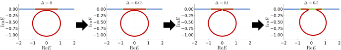
Figure S4: A merging process between the Hatano-Nelson model and the chiral edge mode of the QWZ model ($L_{y}=50,m=-1.5,v=\Gamma=1$).

References

- Bender (2007) C. M. Bender, Reports on Progress in Physics 70, 947 (2007).
- Mostafazadeh and Batal (2004) A. Mostafazadeh and A. Batal, Journal of Physics A: Mathematical and General 37, 11645 (2004).
- Moiseyev (2011) N. Moiseyev, Non-Hermitian quantum mechanics (Cambridge University Press, 2011).
- Ashida et al. (2020) Y. Ashida, Z. Gong, and M. Ueda, Advances in Physics 69, 249 (2020).
- Bergholtz et al. (2021) E. J. Bergholtz, J. C. Budich, and F. K. Kunst, Rev. Mod. Phys. 93, 015005 (2021).
- Okuma and Sato (2023) N. Okuma and M. Sato, Annual Review of Condensed Matter Physics 14, 83 (2023).
- Rudner and Levitov (2009) M. S. Rudner and L. S. Levitov, Phys. Rev. Lett. 102, 065703 (2009).
- Hu and Hughes (2011) Y. C. Hu and T. L. Hughes, Phys. Rev. B 84, 153101 (2011).
- Esaki et al. (2011) K. Esaki, M. Sato, K. Hasebe, and M. Kohmoto, Phys. Rev. B 84, 205128 (2011).
- Schomerus (2013) H. Schomerus, Opt. Lett. 38, 1912 (2013).
- Shen et al. (2018) H. Shen, B. Zhen, and L. Fu, Phys. Rev. Lett. 120, 146402 (2018).
- Yao and Wang (2018) S. Yao and Z. Wang, Phys. Rev. Lett. 121, 086803 (2018).
- Kunst et al. (2018) F. K. Kunst, E. Edvardsson, J. C. Budich, and E. J. Bergholtz, Phys. Rev. Lett. 121, 026808 (2018).
- Yokomizo and Murakami (2019) K. Yokomizo and S. Murakami, Phys. Rev. Lett. 123, 066404 (2019).
- Hatsugai (1993) Y. Hatsugai, Phys. Rev. Lett. 71, 3697 (1993).
- Hasan and Kane (2010) M. Z. Hasan and C. L. Kane, Rev. Mod. Phys. 82, 3045 (2010).
- Qi and Zhang (2011) X.-L. Qi and S.-C. Zhang, Rev. Mod. Phys. 83, 1057 (2011).
- Yao et al. (2018) S. Yao, F. Song, and Z. Wang, Phys. Rev. Lett. 121, 136802 (2018).
- Herviou et al. (2019) L. Herviou, J. H. Bardarson, and N. Regnault, Phys. Rev. A 99, 052118 (2019).
- Song et al. (2019) F. Song, S. Yao, and Z. Wang, Phys. Rev. Lett. 123, 246801 (2019).
- Nakamura et al. (2022) D. Nakamura, T. Bessho, and M. Sato, “Bulk-boundary correspondence in point-gap topological phases,” (2022), arXiv:2205.15635 .
- Schnyder et al. (2008) A. P. Schnyder, S. Ryu, A. Furusaki, and A. W. W. Ludwig, Phys. Rev. B 78, 195125 (2008).
- Kitaev (2009) A. Kitaev, AIP Conference Proceedings 1134, 22 (2009).
- Ryu et al. (2010) S. Ryu, A. P. Schnyder, A. Furusaki, and A. W. Ludwig, New Journal of Physics 12, 065010 (2010).
- Chiu et al. (2016) C.-K. Chiu, J. C. Y. Teo, A. P. Schnyder, and S. Ryu, Rev. Mod. Phys. 88, 035005 (2016).
- Kawabata et al. (2019) K. Kawabata, K. Shiozaki, M. Ueda, and M. Sato, Phys. Rev. X 9, 041015 (2019).
- Gong et al. (2018) Z. Gong, Y. Ashida, K. Kawabata, K. Takasan, S. Higashikawa, and M. Ueda, Phys. Rev. X 8, 031079 (2018).
- Zhou and Lee (2019) H. Zhou and J. Y. Lee, Phys. Rev. B 99, 235112 (2019).
- D. S. Borgnia, and A. J. Kruchkov, and R.-J. Slager (2020) D. S. Borgnia, and A. J. Kruchkov, and R.-J. Slager, Phys. Rev. Lett. 124, 056802 (2020).
- N. Okuma, and M. Sato (2019) N. Okuma, and M. Sato, Phys. Rev. Lett. 123, 097701 (2019).
- Okuma et al. (2020) N. Okuma, K. Kawabata, K. Shiozaki, and M. Sato, Phys. Rev. Lett. 124, 086801 (2020).
- Zhang et al. (2020) K. Zhang, Z. Yang, and C. Fang, Phys. Rev. Lett. 125, 126402 (2020).
- Okuma and Sato (2021) N. Okuma and M. Sato, Phys. Rev. B 103, 085428 (2021).
- Kawabata et al. (2021) K. Kawabata, K. Shiozaki, and S. Ryu, Phys. Rev. Lett. 126, 216405 (2021).
- Yang et al. (2021) Z. Yang, A. P. Schnyder, J. Hu, and C.-K. Chiu, Phys. Rev. Lett. 126, 086401 (2021).
- Vecsei et al. (2021) P. M. Vecsei, M. M. Denner, T. Neupert, and F. Schindler, Phys. Rev. B 103, L201114 (2021).
- Denner et al. (2021) M. M. Denner, A. Skurativska, F. Schindler, M. H. Fischer, R. Thomale, T. Bzdušek, and T. Neupert, Nature communications 12, 5681 (2021).
- Hu et al. (2022) H. Hu, E. Zhao, and W. V. Liu, Phys. Rev. B 106, 094305 (2022).
- Lee et al. (2019a) J. Y. Lee, J. Ahn, H. Zhou, and A. Vishwanath, Phys. Rev. Lett. 123, 206404 (2019a).
- Terrier and Kunst (2020) F. Terrier and F. K. Kunst, Phys. Rev. Res. 2, 023364 (2020).
- Bessho and Sato (2021) T. Bessho and M. Sato, Phys. Rev. Lett. 127, 196404 (2021).
- Lee et al. (2019b) C. H. Lee, L. Li, and J. Gong, Phys. Rev. Lett. 123, 016805 (2019b).
- Luo and Zhang (2019) X.-W. Luo and C. Zhang, Phys. Rev. Lett. 123, 073601 (2019).
- Li et al. (2020) L. Li, C. H. Lee, and J. Gong, Phys. Rev. Lett. 124, 250402 (2020).
- Okugawa et al. (2020) R. Okugawa, R. Takahashi, and K. Yokomizo, Phys. Rev. B 102, 241202 (2020).
- Kawabata et al. (2020) K. Kawabata, M. Sato, and K. Shiozaki, Phys. Rev. B 102, 205118 (2020).
- Fu et al. (2021) Y. Fu, J. Hu, and S. Wan, Phys. Rev. B 103, 045420 (2021).
- Shiozaki and Ono (2021) K. Shiozaki and S. Ono, Phys. Rev. B 104, 035424 (2021).
- Palacios et al. (2021) L. S. Palacios, S. Tchoumakov, M. Guix, I. Pagonabarraga, S. Sánchez, and A. G. Grushin, Nature Communications 12, 4691 (2021).
- Kim and Park (2021) K.-M. Kim and M. J. Park, Phys. Rev. B 104, L121101 (2021).
- Zhang et al. (2021) X. Zhang, Y. Tian, J.-H. Jiang, M.-H. Lu, and Y.-F. Chen, Nature communications 12, 5377 (2021).
- Ghorashi et al. (2021a) S. A. A. Ghorashi, T. Li, M. Sato, and T. L. Hughes, Phys. Rev. B 104, L161116 (2021a).
- Ghorashi et al. (2021b) S. A. A. Ghorashi, T. Li, and M. Sato, Phys. Rev. B 104, L161117 (2021b).
- Zou et al. (2021) D. Zou, T. Chen, W. He, J. Bao, C. H. Lee, H. Sun, and X. Zhang, Nature Communications 12, 7201 (2021).
- Li et al. (2022) Y. Li, C. Liang, C. Wang, C. Lu, and Y.-C. Liu, Phys. Rev. Lett. 128, 223903 (2022).
- Zhu and Gong (2022) W. Zhu and J. Gong, Phys. Rev. B 106, 035425 (2022).
- Denner and Schindler (2023) M. M. Denner and F. Schindler, SciPost Phys. 14, 107 (2023).
- Liu and Fulga (2023) H. Liu and I. C. Fulga, Phys. Rev. B 108, 035107 (2023).
- Shang et al. (2022) C. Shang, S. Liu, R. Shao, P. Han, X. Zang, X. Zhang, K. N. Salama, W. Gao, C. H. Lee, R. Thomale, et al., Advanced Science 9, 2202922 (2022).
- Zhu and Gong (2023) W. Zhu and J. Gong, Phys. Rev. B 108, 035406 (2023).
- Roccati et al. (2023) F. Roccati, M. Bello, Z. Gong, M. Ueda, F. Ciccarello, A. Chenu, and A. Carollo, “Hermitian and Non-Hermitian Topology from Photon-Mediated Interactions,” (2023), arXiv:2303.00762 .
- Nakai et al. (2023) Y. O. Nakai, N. Okuma, D. Nakamura, K. Shimomura, and M. Sato, “Topological enhancement of non-normality in non-Hermitian skin effects,” (2023), arXiv:2304.06689 .
- Hatano and Nelson (1996) N. Hatano and D. R. Nelson, Phys. Rev. Lett. 77, 570 (1996).
- Hatano and Nelson (1997) N. Hatano and D. R. Nelson, Phys. Rev. B 56, 8651 (1997).
- Hatano and Nelson (1998) N. Hatano and D. R. Nelson, Phys. Rev. B 58, 8384 (1998).
- Note (1) For a microscopic derivation of such a dissipation, see Sec.S2 in Supplement Material, which includes Refs. Datta (1995); Aoki et al. (2014).
- Note (2) See Sec.S4 in Supplement Material for a more detailed relation between the Hatano-Nelson model and the chiral edge state with dissipation.
- Qi et al. (2006) X.-L. Qi, Y.-S. Wu, and S.-C. Zhang, Phys. Rev. B 74, 085308 (2006).
- Note (3) See Sec.S1 in Supplement Material for spatial profiles of open boundary modes, which includes Refs. Okuma and Sato (2023); Nakai et al. (2023).
- Altland and Zirnbauer (1997) A. Altland and M. R. Zirnbauer, Phys. Rev. B 55, 1142 (1997).
- Lieu et al. (2020) S. Lieu, M. McGinley, and N. R. Cooper, Phys. Rev. Lett. 124, 040401 (2020).
- Yoshida et al. (2020) T. Yoshida, R. Peters, N. Kawakami, and Y. Hatsugai, Progress of Theoretical and Experimental Physics 2020, 12A109 (2020).
- Note (4) For details, see Sec.S3 in Supplement Material, which includes Ref. Yoshida et al. (2020).
- Sato et al. (2012) M. Sato, K. Hasebe, K. Esaki, and M. Kohmoto, Progress of Theoretical Physics 127, 937 (2012).
- Teo and Kane (2010) J. C. Y. Teo and C. L. Kane, Phys. Rev. B 82, 115120 (2010).
- Pikulin and Nazarov (2013) D. I. Pikulin and Y. V. Nazarov, Phys. Rev. B 87, 235421 (2013).
- San-Jose et al. (2016) P. San-Jose, J. Cayao, E. Prada, and R. Aguado, Scientific reports 6, 21427 (2016).
- Avila et al. (2019) J. Avila, F. Peñaranda, E. Prada, P. San-Jose, and R. Aguado, Communications Physics 2, 133 (2019).
- Liu et al. (2022) H. Liu, M. Lu, Y. Wu, J. Liu, and X. C. Xie, Phys. Rev. B 106, 064505 (2022).
- Note (5) See Sec.S1 in Supplement Material for spatial profiles of open boundary modes, which includes Refs. Okuma and Sato (2023); Nakai et al. (2023).
- Yi and Yang (2020) Y. Yi and Z. Yang, Phys. Rev. Lett. 125, 186802 (2020).
- Sato and Ando (2017) M. Sato and Y. Ando, Reports on Progress in Physics 80, 076501 (2017).
- Ando (2013) Y. Ando, Journal of the Physical Society of Japan 82, 102001 (2013).
- (84) K. Inaka, D. Nakamura, and M. Sato, Japan Physics Society 2023 Spring Meeting, 23pD1-8:unpublished .
- Ma et al. (2023) X. Ma, K. Cao, X. Wang, Z. Wei, and S. Kou, “Chiral Skin Effect,” (2023), arXiv:2304.01422 .
- Schindler et al. (2023) F. Schindler, K. Gu, B. Lian, and K. Kawabata, PRX Quantum 4, 030315 (2023).
- Datta (1995) S. Datta, Electronic Transport in Mesoscopic Systems, Cambridge Studies in Semiconductor Physics and Microelectronic Engineering (Cambridge University Press, 1995).
- Aoki et al. (2014) H. Aoki, N. Tsuji, M. Eckstein, M. Kollar, T. Oka, and P. Werner, Rev. Mod. Phys. 86, 779 (2014).