Visualizing hypothesis tests in survival analysis under anticipated delayed effects

Abstract

What can be considered an appropriate statistical method for the primary analysis of a randomized clinical trial (RCT) with a time-to-event endpoint when we anticipate non-proportional hazards owing to a delayed effect? This question has been the subject of much recent debate. The standard approach is a log-rank test and/or a Cox proportional hazards model. Alternative methods have been explored in the statistical literature, such as weighted log-rank tests and tests based on the Restricted Mean Survival Time (RMST). While weighted log-rank tests can achieve high power compared to the standard log-rank test, some choices of weights may lead to type-I error inflation under particular conditions. In addition, they are not linked to an unambiguous estimand. Arguably, therefore, they are difficult to intepret. Test statistics based on the RMST, on the other hand, allow one to investigate the average difference between two survival curves up to a pre-specified time point $\tau$ – an unambiguous estimand. However, by emphasizing differences prior to $\tau$, such test statistics may not fully capture the benefit of a new treatment in terms of long-term survival. In this article, we introduce a graphical approach for direct comparison of weighted log-rank tests and tests based on the RMST. This new perspective allows a more informed choice of the analysis method, going beyond power and type I error comparison.

Keywords Delayed effects, Pseudo-value, Score, Survival test, Visualization

1 Introduction

Delayed effects are a well-known form of non-proportional hazards typically linked to checkpoint inhibitors in immuno-oncology (IO). In a randomized clinical trial (RCT) comparing chemotherapy with an IO compound, we may well expect the Kaplan-Meier curves to remain close to equal for some time before they diverge. One potential explanation for this behavior is that an IO agent does not target the tumor directly; it instead boosts the patient’s immune system, and this positive effect may not be observed immediately. The lag between the activation of immune cells, their proliferation and impact on the tumor is described in the literature as a delayed treatment effect.

There is an ongoing debate about what should be considered an appropriate primary analysis for such trials, in particular whether to keep the log-rank test (or the Cox model) as a de-facto standard, or to employ alternative methods (Freidlin and Korn, 2019; Uno and Tian, 2020; Huang et al., 2020; Freidlin and Korn, 2020). Recent publications (e.g., Lin et al. (2020); Royston and B Parmar (2020); Chen et al. (2020); Jiménez et al. (2019); Jiménez (2022); Roychoudhury et al. (2021); Mukhopadhyay et al. (2022)) suggest that alternative testing methods, for example weighted log-rank tests, are better tailored for settings with non-proportional hazards, based largely on the fact that they can achieve higher power. This view has been challenged, however, on at least two grounds. Firstly, some of the proposed methods have been shown to produce counter-intuitive results. For example, Freidlin and Korn (2019) construct a scenario in which the experimental treatment is uniformly worse than control, and yet a particular choice of weighted log-rank test would have a high chance of rejecting the null hypothesis in favour of the experimental treatment. Secondly, weighted log-rank tests are not constructed around an unambiguous estimand. Huang et al. (2020) argue that, as a matter of principle, the primary analysis of an RCT should be an estimation procedure with a corresponding confidence interval. Application of this principle would rule out a weighted log-rank test. In the case of non-proportional hazards, Huang et al. (2020) recommend to estimate the difference in restricted mean survival time (RMST) between the two arms. Another potential estimand would be the difference in survival probabilities at a specific time, a so-called milestone analysis.

We do not hope to settle this debate in this article. Instead, our aim is to develop graphical comparisons of the various testing methods, deepening our understanding of how they work. To do so, we follow Magirr and Burman (2019) and represent a weighted log-rank test statistic as a difference in mean score between the two treatment arms. We then show that we can express tests that are based on the Kaplan-Meier estimates of the restricted mean survival time (RMST) and milestone survival probabilities in the same way via the concept of “pseudo-values” or “pseudo-observations” proposed by Andersen et al. (2003). This allows us to put both the weighted log-rank tests and the methods derived from the Kaplan-Meier curves in a common framework which makes them directly comparable. Furthermore, we provide an R package, publicly available on CRAN, to make the proposed methods effectively reproducible.

The rest of the article is organized as follows. In Section 2 we introduce the POPLAR trial that we use to illustrate the common visualization framework proposed in this article. In Section 3, we introduce the basic theory behind weighted log-rank tests and the tests based on the RMST and milestone survival probabilities, as well as how to represent them as between-arm differences in mean scores and pseudo-values, respectively. In Section 4, we present the graphical comparison of the various survival tests. We conclude the article in Section 5 with a discussion and some final remarks.

2 The POPLAR trial (NCT01903993)

We shall use the POPLAR trial (Fehrenbacher et al. (2016)) as a starting point for our discussion. This was an open-label phase 2 randomized controlled trial of atezolizumab versus docetaxel for patients with previously-treated non-small-cell lung cancer. Key design assumptions and de-identified data are publicly available (Gandara et al. (2018)). The sample size was calculated assuming a median overall survival (OS) of 8 months for the control arm and a HR of 0.65, which translated into an assumed median OS of approximately 12.3 months for the atezolizumab arm, under an exponential model. Recruitment lasted 8 months. Three interim analyses were planned, with (two-sided) alpha levels of 0.0001, 0.0001, and 0.001. The final analysis of OS was performed when 173 deaths had occurred in the intention-to-treat (ITT) population, using a two-sided $\alpha$ level of 4.88%. The trial enrolled a total of 287 patients. A Kaplan-Meier estimate derived from the published data set Gandara et al. (2018) is shown in Figure 1, where a delayed effect is identifiable.

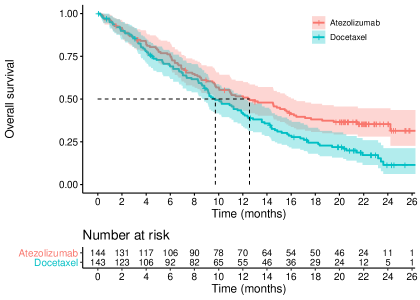
Figure 1: Kaplan-Meier curves from the POPLAR trial.

3 Methods

3.1 Weighted log-rank tests

To implement a weighted log-rank test, we scan over the ordered unique event times $t_{1},t_{2},\ldots,t_{J}$, and take a weighted sum of the observed minus expected events on one of the treatment arms, where the expectation is taken assuming that the survival distributions on the two arms are identical. Let $n_{i,j}$ denote the number of patients at risk on treatment $i=0,1$ just prior to time $t_{j}$, and let $O_{i,j}$ denote the observed number of events on treatment $i=0,1$ at time $t_{j}$, with the expected number of events given by $E_{i,j}=O_{j}\times n_{i,j}/n_{j}$, where $n_{j}=n_{0,j}+n_{1,j}$ and $O_{j}=O_{0,j}+O_{1,j}$. The weighted log-rank test statistic is defined as

$$U_{W}:=\sum_{j=1}^{J}w_{j}\left(O_{1,j}-E_{1,j}\right)\sim N(0,V_{W}),$$

where

$$V_{W}=\sum_{j=1}^{J}w_{j}^{2}\frac{n_{0,j}n_{1,j}O_{j}(n_{j}-O_{j})}{n_{j}^{2}(n_{j}-1)},$$

and $w_{j}$ represents the weight at time $t_{j}$.

If the experimental treatment is beneficial compared to the control treatment, we should see fewer events on the experimental arm than would be expected assuming identical survival curves on the two treatments, leading to $U_{W}<<0$. The one-sided p-value is calculated as $p_{W}=\Phi(U_{W}/\sqrt{V_{W}})$, where $\Phi(.)$ represents the cumulative distribution function of the standard Normal distribution.

A weighted log-rank test allows one to pre-specify the weights to boost the chances that $p<\alpha$, given the expected treatment effect. In other words, because of the anticipated delayed Kaplan-Meier curves separation, we will choose the weights in a way that early events, that occur when the Kaplan-Meier curves are expected to be similar to each other, are underweighted compared to late events. Fleming and Harrington (2011) proposed a class of weight functions with $w_{j}=(\hat{S}(t_{j}-))^{\rho}\times(1-\hat{S}(t_{j}-))^{\gamma}$, where $\hat{S}(t_{j}-)$ is the Kaplan-Meier estimate of the pooled sample just prior to time $t_{j}$. Under anticipated delayed treatment effects, a popular choice is the Fleming-Harrington-(0,1) test, which uses $\rho=0$, $\gamma=1$ and therefore the weight $w_{j}=1-\hat{S}(t_{j}-)$. A recently proposed alternative to the Fleming-Harrington class of weights is the modestly-weighted log-rank test (see Magirr and Burman (2019)), which uses $w_{j}=1/\max{\left\{\widehat{S}(t_{j}-),s^{*}\right\}}$, for fixed $s^{*}$. In common with the Fleming-Harrington-(0,1) test, it gives relatively larger weight to later events than to earlier events, but it has the advantage that it controls the type-I error rate not only for the sharp null hypothesis $H_{0}:S_{1}(t)=S_{0}(t)~{}\forall~{}t$ but also for the strong null $\tilde{H}_{0}:S_{1}(t)\leq S_{0}(t)~{}\forall~{}t$. The first event receives a weight of 1, and weights are increasing up to a maximum $1/s^{*}$. So choosing $s^{*}=0.5$, for example, allows the weights to range from 1 to 2 (assuming that event rates are such that $\widehat{S}(t)=0.5$ for some $t$) which may be a reasonable choice in many immuno-oncology trials. Choosing $s^{*}\approx 1$ makes the test more similar to a standard log-rank test. A tutorial on how to design a randomized clinical trial using the modestly weighted log-rank test was recently published by Magirr and Jiménez (2022).

Although weighted log-rank tests are usually thought of as a weighted sum of observed minus expected events, they can also be expressed as a difference in mean score on the two treatment arms Leton and Zuluaga (2001); Magirr (2021). Letting $l_{1,j}$ and $l_{0,j}$ denote the number of patients censored on the test treatment and control treatment, respectively, during $\left[\left.t_{j},t_{j+1}\right)\right.$, we can express the weighted log-rank statistic as

$$\begin{split}U_{W}&:=\sum_{j=1}^{J}w_{j}\left(O_{1,j}-O_{j}\frac{n_{1,j}}{n_{j}}\right)\\ &=\sum_{j=1}^{J}w_{j}O_{1,j}-\sum_{j=1}^{J}w_{j}\frac{O_{j}}{n_{j}}\times n_{1,j}\\ &=\sum_{j=1}^{J}w_{j}O_{1,j}-\sum_{j=1}^{J}w_{j}\frac{O_{j}}{n_{j}}\times\sum_{i=j}^{J}(O_{1,i}+l_{1,i})\\ &=\sum_{j=1}^{J}w_{j}O_{1,j}-\sum_{j=1}^{J}(O_{1,j}+l_{1,j})\times\sum_{i=1}^{J}w_{i}\frac{O_{i}}{n_{i}}\\ &=\sum_{j=1}^{J}O_{1,j}\left(w_{j}-\sum_{i=1}^{j}w_{i}\frac{O_{i}}{n_{i}}\right)+\sum_{j=1}^{J}l_{1,j}\left(-\sum_{i=1}^{j}w_{i}\frac{O_{i}}{n_{i}}\right).\\ \end{split}$$ (1)

The final expression in (1) can also be written as a sum of "scores", $a_{k}$, over all patients $k=1,\ldots,N$

$$U_{W}=\sum_{k=1}^{N}\mathbb{I}\left\{z_{k}=1\right\}a_{k}$$

where $z_{k}$ denotes the treatment assignment of patient $k$. If patient $k$ has an event at time $t_{j}$, then they are given a score of $a_{k}:=w_{j}-\sum_{i=1}^{j}w_{i}\frac{O_{i}}{n_{i}}$, where the summation is over the observed event times up to time $t_{j}$. If, instead, patient $k$ had a censored observation during $\left[\left.t_{j},t_{j+1}\right)\right.$ they would receive a score of $a_{k}:=-\sum_{i=1}^{j}w_{i}\frac{O_{i}}{n_{i}}$.

The estimator $V_{W}$ for the variance of $U_{W}$ is usually derived from a sampling viewpoint. It can be arrived at via a Cox model with treatment term only. When we fit a Cox model, we consider the variance of $U_{W}$ under repeated iterations of the experiment from the same (super)population. When we express $U_{W}$ as a sum of scores, however, it shifts us towards a randomization inference perspective. That is, we consider the sample fixed, and the only source of randomness is the treatment assignment. Under this framework, and indexing the patients such that the first $k=1,\ldots,N_{1}$ patients are those on treatment $1$, another way to express $U_{W}$ is

$$U_{W}=\sum_{k=1}^{N_{1}}A_{l}$$

where the $A_{1},\ldots,A_{N_{1}}$ are a random sample of size $N_{1}$ from $a_{1},\ldots,a_{N}$. In particular,

$$p(A_{k}=a)=\frac{1}{N},\text{ for }a=a_{1},\ldots,a_{N}$$

and

$$p(A_{k}=a,A_{l}=a^{\prime})=\left\{\begin{array}[]{c c}\frac{1}{N(N-1)}&\text{ for }a\neq a^{\prime}\\ 0&\text{otherwise.}\end{array}\right.$$

Also note that $\sum_{k=1}^{N}a_{k}=0$, as can be seen by switching the treatment labels in (1),

$$\begin{split}\sum_{k=1}^{N}\mathbb{I}\left\{z_{k}=1\right\}a_{k}+\sum_{k=1}^{N}\mathbb{I}\left\{z_{k}=0\right\}a_{k}&=\sum_{j=1}^{J}w_{j}\left(O_{1,j}-O_{j}\frac{n_{1,j}}{n_{j}}\right)+\sum_{j=1}^{J}w_{j}\left(O_{0,j}-O_{j}\frac{n_{0,j}}{n_{j}}\right)\\ &=0.\end{split}$$ (2)

Thus,

$$E(A_{k})=\frac{1}{N}\sum_{i=1}^{N}a_{k}=0,$$

$$Var(A_{k})=\frac{1}{N}\sum_{i=1}^{N}a_{k}^{2},$$

and

$$\begin{split}Cov(A_{k},A_{l})&=E(A_{k}A_{l})\\ &=\frac{1}{N(N-1)}\sum_{k\neq l}a_{k}a_{l}\\ &=\frac{1}{N(N-1)}\left\{\left(\sum_{k=1}^{N}a_{k}\right)^{2}-\sum_{k=1}^{N}a_{k}^{2}\right\}\\ &=\frac{-1}{N(N-1)}\sum_{i=1}^{N}a_{k}^{2}.\end{split}$$

It follows that $E_{P}(U_{W})=0$ and

$$\begin{split}Var_{P}(U_{W})&=\sum_{k=1}^{N_{1}}Var(A_{k})+\sum_{k\neq l}Cov(A_{k},A_{l})\\ &=\frac{N_{1}}{N}\sum_{k=1}^{N}a_{k}^{2}-\frac{N_{1}^{2}-N_{1}}{N(N-1)}\sum_{k=1}^{N}a_{k}^{2}\\ &=\frac{N_{1}(N-1)-(N_{1}^{2}-N_{1})}{N(N-1)}\sum_{k=1}^{N}a_{k}^{2}\\ &=\frac{N_{1}(N-N_{1})}{N(N-1)}\sum_{k=1}^{N}a_{k}^{2},\end{split}$$

where we use the subscript $P$ to emphasize this refers to the permutation distribution of $U_{W}$. Note that instead of using $U_{W}$, we could just as well use the difference in mean score on the two arms,

$$\begin{split}\tilde{U}_{W}&=\frac{\sum_{k=1}^{N}\mathbb{I}\left\{z_{k}=1\right\}a_{k}}{N_{1}}-\frac{\sum_{i=1}^{N}\mathbb{I}\left\{z_{k}=0\right\}a_{k}}{N-N_{1}}\\ &=\frac{U_{W}}{N_{1}}-\frac{\sum_{k=1}^{N}a_{k}-U_{W}}{N-N_{1}}\\ &=U_{W}\left(\frac{1}{N_{1}}+\frac{1}{N-N_{1}}\right)\end{split}$$ (3)

as the test statistic, with $E_{P}(\tilde{U}_{W})=0$ and $Var_{P}(\tilde{U}_{W})=(N_{1}^{-1}+(N-N_{1})^{-1})^{2}Var_{P}(U_{W})$.

It can be shown that, asymptotically, $\tilde{U}_{W}\sim N(0,Var_{P}(\tilde{U}_{W}))$, and this could be used for inference. Alternatively, one could compute an exact p-value by considering all permutations of the treatment labels. Also, although $V_{W}$ and $Var_{P}(U_{W})$ are derived via different frameworks, it can be shown that they are approximately the same when the censoring distribution is the same on the two arms (Leton and Zuluaga, 2001), as should usually be the case for administrative censoring in an RCT. One may perform the weighted log-rank test with variance estimator $V_{W}$ but keeping in mind the permutation interpretation to gain insight into how the test statistic behaves.

To make it easier to visually compare scores from different weighted tests we can also perform a re-scaling

$$b_{k}=\frac{2a_{k}-\max{a}-\min{a}}{\max{a}-\min{a}}$$

so that the standardized scores $b_{k}\in(-1,1)$. This leaves the p-value of the permutation test unchanged.

3.2 Tests based on the Restricted Mean Survival Time (RMST) and Milestone survival rates

The $\tau$-restricted mean survival time (RMST) is defined as $\mbox{RMST}(\tau)=E(\min\left\{T,\tau\right\})=\int_{0}^{\tau}S(t)dt$, where $S(t)=P(T>t)=\exp\left(-\int_{0}^{t}\lambda(u)du\right)$ is the survival function and $\lambda(t)$ the hazard function (Royston and Parmar (2011); Tian et al. (2014)). The RMST represents the expected lifetime over a time horizon equal to $\tau$, that in the context of the primary analysis of a clinical trial would have to be pre-specified. The test statistic linked to the difference between the RMST of the experimental and control arms is usually based on the Kaplan-Meier estimator and calculated as follows. With notation introduced in Section 3.1, let $U_{\mbox{RMST}}=\int_{0}^{\tau}\left(\widehat{S}_{\mbox{1}}(t)-\widehat{S}_{\mbox{0}}(t)\right)dt$ be the difference in estimated RMST on treatment and control arms, respectively, and $V_{\mbox{RMST}}=\sum_{i=0,1}\sum_{j=1}^{J}(\int_{t_{j}}^{\tau}\widehat{S}_{i}(t)dt)^{2}\frac{O_{i,j}}{n_{i,j}(n_{i,j}-O_{i,j})}$ its variance. The one-sided p-value is calculated as $p_{\mbox{RMST}}=\Phi(-U_{\mbox{RMST}}/\sqrt{V_{\mbox{RMST}}})$.

Milestone survival analysis (Klein et al. (2007)) compares survival probabilities at a fixed point in time $\kappa$. Let $U_{\mbox{MLST}}=\widehat{S}_{1}(\kappa)-\widehat{S}_{0}(\kappa)$ be the difference between the estimated survival probabilities at time $\kappa$ on treatment and control arms, respectively, and $V_{\mbox{MLST}}=\sum_{i=0,1}\sum_{t_{j}\leq\kappa}\widehat{S}_{i}(\kappa)^{2}\frac{O_{i,j}}{n_{i,j}(n_{i,j}-O_{i,j})}$ its variance. The one-sided p-value is calculated as $p_{\mbox{MLST}}=\Phi(-U_{\mbox{MLST}}/\sqrt{V_{\mbox{MLST}}})$.

In these forms, the RMST and the milestone analysis are difficult to compare with a weighted log-rank test. However, these two analyses, that traditionally employ Kaplan-Meier estimators, can also be addressed with the use of pseudo-values (Andersen et al. (2003)) in such a way that the pseudo-values are directly analogous with the scores derived for the weighted log-rank test.

For the RMST($\tau$), the $k$-th pseudo-value, $k=1,\ldots,N$, is defined as

$$\theta_{k}^{\mbox{RMST},\tau}=N\int_{0}^{\tau}\widehat{S}(t)dt-(N-1)\int_{0}^{\tau}\widehat{S}^{(-k)}(t)dt,$$ (4)

where $\widehat{S}^{(-k)}(t)$ is the Kaplan-Meier estimator excluding patient $k$. It can be shown (Graw et al., 2009; Jacobsen and Martinussen, 2016; Overgaard et al., 2017) that, asymptotically,

$$E(\theta_{k}^{\mbox{RMST},\tau}\mid Z_{k})\approx E(\min\left\{T_{k},\tau\right\}\mid Z_{k}),$$ (5)

where $Z_{k}$ denotes treatment assignment. Thus, one may estimate the difference in RMST($\tau$) between the two arms as

$$\tilde{U}_{\mbox{RMST},\tau}=\frac{\sum_{k=1}^{N}\mathbb{I}\left\{z_{k}=1\right\}\theta_{k}^{\mbox{RMST},\tau}}{N_{1}}-\frac{\sum_{k=1}^{N}\mathbb{I}\left\{z_{k}=0\right\}\theta_{k}^{\mbox{RMST},\tau}}{N-N_{1}}$$

For the purpose of testing the null hypothesis $H_{0}:S_{1}(t)=S_{0}(t)~{}\forall~{}t$, the statistic $\tilde{U}_{\mbox{RMST}}$ is directly analagous to $\tilde{U}_{W}$ in (3), with the pseudovalues $\theta_{k}^{\mbox{RMST},\tau}$ playing the role of the $a_{k}$. It is usually recommended to estimate the variance of $\tilde{U}_{\mbox{RMST}}$ via non-parametric bootstrap or using a robust variance estimator for a linear model. In principle, for the purpose of testing the null hypothesis $H_{0}$, one could switch to a randomization inference perspective and consider the permutation distribution of $\tilde{U}_{\mbox{RMST}}$, as has been previously suggested by Horiguchi and Uno (2020). In this case, one is free to re-scale the pseudo-values without it changing the p-value. As mentioned in Section 3.1, one does not have to actually implement the permutation test in order to benefit from the additional insight it provides. By comparing (re-scaled versions) of $\theta_{k}^{\mbox{RMST},\tau}$ and $a_{k}$, we can better understand the behaviour of the respective tests. It is important to note, of course, that the usefulness of $\tilde{U}_{\mbox{RMST},\tau}$ goes beyond testing the null hypothesis, since it provides us with a point estimate and confidence interval for a meaningful estimand (although one would typically use the Kaplan-Meier based estimators instead). We shall pick up on this aspect in the Section 5.

For the milestone analysis, the procedure is exactly the same as for RMST, but with pseudo values defined as

$$\theta_{k}^{\mbox{MLST},\kappa}=n\widehat{S}(\kappa)-(n-1)\widehat{S}^{(-k)}(\kappa).$$ (6)

We shall furthermore consider two novel estimands that can be estimated in the same way via the Kaplan-Meier estimator. Firstly, the between-arm difference in window mean survival time (Paukner and Chappell (2021)), otherwise known as long-term restricted mean survival time (Horiguchi et al. (2023)). The window mean survival time (WMST) is defined as WMST($\tau_{1}$, $\tau_{2}$) = RMST($\tau_{2}$) - RMST($\tau_{1}$) for $\tau_{2}>\tau_{1}$. It has the interpretation of the mean amount of time spent alive between $\tau_{1}$ and $\tau_{2}$. The second novel estimand proposed by Uno and Horiguchi (2023) and Snapinn et al. (2023) is the between-arm difference in the (log) average hazard with survival weight (AHSW). The AHSW is defined as AHSW($\tau$) = (1 - S($\tau$)) / RMST($\tau$). It can be interpreted as "the average person-time incidence rate of $T$ on $t\in(0,\tau)$ when all $T$ before $\tau$ would have been observed without being censored by study-specific censoring time" (Uno and Horiguchi (2023)). For both of these novel estimands, the procedure for calculating pseudo-values and estimating between-arm differences is analogous to the procedure for RMST.

The concept of pseudo-values can also be extended to parametric estimators of the survival curve Nygård Johansen et al. (2020), simply by replacing the Kaplan-Meier estimator $\widehat{S}(t)$ with its parametric equivalent. This is something we shall also explore in Section 4.

4 Graphical comparison

In this section, we use the POPLAR trial data described in Section 2 to run a series of survival tests and observe how they behave under the lens of the (re-scaled) scores for the weighted log-rank tests, and the (re-scaled) pseudo-values for the tests based on the RMST and Milestone survival rates. By comparing tests in a number of ways we derive several insights.

4.1 Modestly weighted log-rank tests

In Figure 2, we plot the scores from the modestly-weighted log-rank test (with $s^{*}=0.5$) side-by-side with those from the standard log-rank test, and also with those from Kaplan-Meier and parametric-based milestone analysis at 18 months. The modestly-weighted test appears to be a compromise between the log-rank test and the Kaplan-Meier based milestone analysis, in the sense that the scores for observed events are approximately equal to 1 for an initial period (similar to the milestone analysis) before steadily decreasing for later follow-up times (similar to a log-rank test). With the Kaplan-Meier based milestone analysis there is a sharp dichotomy; events just before and just after the milestone are given extreme opposite scores. The dangers of outcome dichotomization in terms of loss of information are well documented (Senn, 2005; Fedorov et al., 2009). One way to avoid this loss of information is to apply parametric models instead of the non-parametric Kaplan-Meier estimator Nygård Johansen et al. (2020). Three model-based approaches are shown in the bottom row of Figure 2. The first uses an exponential model, producing scores that look almost identical to the log-rank scores. The second uses a piecewise exponential model with breakpoints at 2, 4, 6 and 8 months, while the third uses a flexible parametric model with a cubic spline on the baseline cumulative hazard (Jackson, 2016). Both of these more flexible models produce scores that look remarkably like those of the modestly-weighted test.

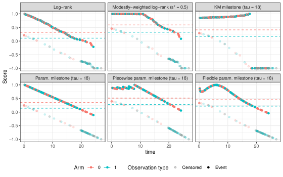
Figure 2: Graphical representation of a modestly-weighted log-rank test, as compared to the log-rank test and milestone analysis, when applied to the POPLAR data. A standardized score is plotted for each patient, where censored observations are semi-transparent. Horizontal dashed lines are plotted at the mean score on each arm. The distance between these two lines corresponds to the numerator in the permutation-based test statistic.

4.2 RMST vs log-rank

In Figure 3, we plot the scores from the Kaplan-Meier based RMST(24) analysis side-by-side with those from the standard log-rank test, and also with those from a Fleming-Harrington-(1,0) test. The RMST test looks more similar to the Fleming-Harrington-(1,0) test than to the standard log-rank test. When interpreting the graphs, the relative vertical distance between a point and the average score lines is indicative of how influential that point is. For the RMST and FH(1,0) tests these distances are greater at earlier timepoints than at later timepoints, whereas for the log-rank test these distances are greater at later timepoints. So the RMST and FH(1,0) tests are giving greater emphasis to early follow-up times, relative to the log-rank test.

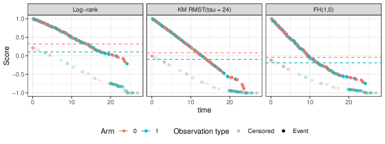
Figure 3: Graphical representation of a test based on the difference in restricted mean survival time (RMST) using Kaplan-Meier derived pseudovalues, as compared to the log-rank test and the Fleming-Harrington-(0,1) test, when applied to the POPLAR data. A standardized score is plotted for each patient, where censored observations are semi-transparent. Horizontal dashed lines are plotted at the mean score on each arm. The distance between these two lines corresponds to the numerator in the permutation-based test statistic.

4.3 Tests based on novel estimands

In Section 3.2, we described two novel estimands that could be estimated via pseudo-values derived from the Kaplan-Meier estimator of survival in the full data. These were the difference in window-mean survival time (WMST) and the difference in average hazard with survival weight (AHSW). Standardized pseudo-values that could be used to test the null hypothesis $H_{0}$ are plotted in Figure 4. The WMST-based test looks somewhat similar to the modestly-weighted test, except that late censored observations are given the same score as late events. We see the same thing when comparing the AHSW-based test with the log-rank test.

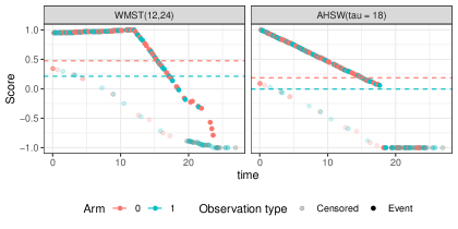
Figure 4: Graphical representation of tests based on the difference in window mean survival time (WMST) and (log) average hazard with survival weight (AHSW) using Kaplan-Meier derived pseudovalues, when applied to the POPLAR data. A standardized score is plotted for each patient, where censored observations are semi-transparent. Horizontal dashed lines are plotted at the mean score on each arm. The distance between these two lines corresponds to the numerator in the permutation-based test statistic.

4.4 Fleming-Harrington-($\rho$, $\gamma$) tests with $\gamma>0$

In Figure 5, we plot the scores from a series of Fleming-Harrington-($\rho$, $\gamma$) tests with $\gamma>0$. The pattern of the scores is strikingly different to the other tests in that they are highly non-monotonic in time. The scores for the group of patients with early events are lower, i.e., better, than the scores of many patients with later events. This leads to the strange behaviour and lack of strong type 1 error control that has previously been observed when using these test statistics Freidlin and Korn (2019); Magirr (2021).

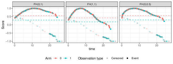
Figure 5: Graphical representation of Fleming-Harrington-($\rho$,$\gamma$) tests, when applied to the POPLAR data. A standardized score is plotted for each patient, where censored observations are semi-transparent. Horizontal dashed lines are plotted at the mean score on each arm. The distance between these two lines corresponds to the numerator in the permutation-based test statistic.

4.5 Effect of early censoring

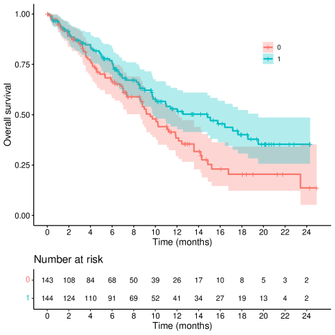
Figure 6: Kaplan-Meier plot from the POPLAR trial data with artificial independent censoring.

It is clear from Figure 1, and from the score plots, that the POPLAR trial had little early censoring. The vast majority of censoring events occur after 20 months, suggesting recruitment lasted approximately 6 months. It may be interesting, however, to understand the behaviour of the test statistics when there is more heavy early censoring. For example, had the recruitment rate been very slow. For this purpose, we artificially mimick a 26 month recruitment period by simulating a competing censoring event from a uniform distribution on (0, 26) months. The resulting data set is shown in Figure 6. Then, in Figure 7, we repeat the score plots for a selection of test statistics when applied to the modified data set. We observe that for the log-rank and weighted log-rank test, the shape of scores over time is qualitatively the same as for the original data set, only with lower density at later follow-up times. The same is true for the parametric milestone analysis based on an exponential distribution. For the Kaplan-Meier based tests, however, we can clearly see that early events have become relatively less influential compared to later events. Intuitively this makes sense. For tests that are anchored to a particular (late) timepoint, if there are relatively few events close to that timepoint then they must naturally have a larger influence on the test statistic. The same is true for the flexible parametric milestone analysis. The exponential-model-based milestone analysis avoids this only by making the strong assumption of constant hazard rates. Note that several of the tests have scores that are non-monotonic in time. This demonstrates that non-monotonicity per-se does not imply the test statistic fails to control the type 1 error rate under the strong null hypothesis. The difference here compared to the situation in Figure 5 is that the non-monoticity is a consequence of censoring. Early events may get lower scores than some later events, but there are now relatively more early events than later events due to censoring.

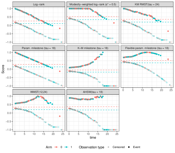
Figure 7: Graphical representation of selected test statistics, when applied to the POPLAR data with additional artificial censoring, as depicted in Figure 6. A standardized score is plotted for each patient, where censored observations are semi-transparent. Horizontal dashed lines are plotted at the mean score on each arm. The distance between these two lines corresponds to the numerator in the permutation-based test statistic.

5 Discussion

The choice of appropriate statistical methodology for the primary analysis of a confirmatory clinical trial is always complex. This is especially the case for time-to-event data, and even more so when we anticipate non-proportional hazards. There are many factors to consider. What is the power, and the type 1 error rate, under a range of plausible assumptions? How easy is it to interpret the output? How easy is it to describe the method in a pre-specified analysis plan? Etc. It is unlikely that there is a single method that is uniformly best across all these diverse criteria. Hence the chosen method(s) must be based on a pragmatic compromise.

When looking at the methods described in this paper, there is one clear differentiating factor. The RMST and milestone analyses involve an unambiguous estimand; the weighted log-rank tests do not. Some statisticians argue, as a matter of principle, that the primary analysis of an RCT should be an estimation procedure for an unambiguous single number summary measure (Huang et al., 2020; Snapinn et al., 2021; Paukner and Chappell, 2022). One could argue that the ICH E9 addendum on estimands (The International Council for Harmonisation of Technical Requirements for Pharmaceuticals for Human Use, 2019) takes this position for granted, although the main ICH E9 guidance on statistical principles in clinical trials (The International Council for Harmonisation of Technical Requirements for Pharmaceuticals for Human Use, 1998) is more open: "The statistical section of the protocol should specify the hypotheses that are to be tested and/or the treatment effects which are to be estimated in order to satisfy the primary objectives of the trial".

The argument to focus on estimation rather than testing is strong. Nevertheless, in the specific case of delayed effects in immuno-oncology, the Kaplan-Meier-based RMST and milestone analyses may involve a large loss of power relative to a well-chosen weighted log-rank test. As we have shown above, when early censoring is low, the RMST analysis emphasizes early differences in survival, where treatment differences are expected to be small. A milestone analysis, on the other hand, may lose power owing to an information-leaking dichotomization. A flexible parametric model might solve the latter issue but is difficult to fully pre-specify in a statistical analysis plan. The restriction time $\tau$ is also difficult to pre-specify, owing to uncertainties in the recruitment rate and survival distributions. It may in some circumstances be possible to make the restriction time data dependent (Tian et al., 2020), although this complicates the definition of the estimand. Similarly, one might argue that novel estimands such as WMST and AHSW no longer have a simple interpretation.

With the help of the graphical representations introduced in this paper, one can show that certain choices of weighted log-rank test are qualitatively similar to tests based on the estimation of familiar estimands. This helps us to understand what the weighted tests are doing and interpret the results correctly. The graphical comparisons can be implemented using the R package nphRCT (Magirr and Barrott (2022)).

While helpful, the tools we introduce here do not provide definitive answers on which methods are acceptable for primary analysis in a given context. There are further factors that we have not considered, for example, how compatible are the methods with stratification, covariate adjustment or missing data imputation? Can the methods be implemented in the context of a group-sequential design? Etc. The choice may well come down to which property one is most willing to sacrifice out of robust power, strict type 1 error control, or unambiguous single-number summary statistic.

Data availability

Software in the form of an R package, together with a vignette and complete documentation are available on CRAN at https://cran.r-project.org/web/packages/nphRCT/index.html. Code to reproduce all outputs can be found at https://github.com/dominicmagirr/visualizing_survival_tests.git.

References

- Andersen et al. [2003] Per Kragh Andersen, John P Klein, and Susanne Rosthøj. Generalised linear models for correlated pseudo-observations, with applications to multi-state models. Biometrika, 90(1):15–27, 2003.
- Chen et al. [2020] Xiaotian Chen, Xin Wang, Kun Chen, Yeya Zheng, Richard J Chappell, and Jyotirmoy Dey. Comparison of survival distributions in clinical trials: A practical guidance. Clinical Trials, 17(5):507–521, 2020.
- Fedorov et al. [2009] Valerii Fedorov, Frank Mannino, and Rongmei Zhang. Consequences of dichotomization. Pharmaceutical Statistics: The Journal of Applied Statistics in the Pharmaceutical Industry, 8(1):50–61, 2009.
- Fehrenbacher et al. [2016] Louis Fehrenbacher, Alexander Spira, Marcus Ballinger, Marcin Kowanetz, Johan Vansteenkiste, Julien Mazieres, Keunchil Park, David Smith, Angel Artal-Cortes, Conrad Lewanski, et al. Atezolizumab versus docetaxel for patients with previously treated non-small-cell lung cancer (poplar): a multicentre, open-label, phase 2 randomised controlled trial. The Lancet, 387(10030):1837–1846, 2016.
- Fleming and Harrington [2011] Thomas R Fleming and David P Harrington. Counting processes and survival analysis. John Wiley & Sons, 2011.
- Freidlin and Korn [2019] Boris Freidlin and Edward L Korn. Methods for accommodating nonproportional hazards in clinical trials: ready for the primary analysis? Journal of Clinical Oncology, 37(35):3455, 2019.
- Freidlin and Korn [2020] Boris Freidlin and Edward L Korn. Reply to h. uno et al and b. huang et al. Journal of Clinical Oncology, 38(17):2003–2004, 2020.
- Gandara et al. [2018] David R Gandara, Sarah M Paul, Marcin Kowanetz, Erica Schleifman, Wei Zou, Yan Li, Achim Rittmeyer, Louis Fehrenbacher, Geoff Otto, Christine Malboeuf, et al. Blood-based tumor mutational burden as a predictor of clinical benefit in non-small-cell lung cancer patients treated with atezolizumab. Nature medicine, 24(9):1441–1448, 2018.
- Graw et al. [2009] Frederik Graw, Thomas A Gerds, and Martin Schumacher. On pseudo-values for regression analysis in competing risks models. Lifetime Data Analysis, 15(2):241–255, 2009.
- Horiguchi and Uno [2020] Miki Horiguchi and Hajime Uno. On permutation tests for comparing restricted mean survival time with small sample from randomized trials. Statistics in Medicine, 39(20):2655–2670, 2020.
- Horiguchi et al. [2023] Miki Horiguchi, Lu Tian, and Hajime Uno. On assessing survival benefit of immunotherapy using long-term restricted mean survival time. Statistics in Medicine, 2023.
- Huang et al. [2020] Bo Huang, Lee-Jen Wei, and Ethan B Ludmir. Estimating treatment effect as the primary analysis in a comparative study: moving beyond p value. Journal of clinical oncology: official journal of the American Society of Clinical Oncology, 38(17):2001–2002, 2020.
- Jackson [2016] Christopher H Jackson. flexsurv: a platform for parametric survival modeling in r. Journal of statistical software, 70, 2016.
- Jacobsen and Martinussen [2016] Martin Jacobsen and Torben Martinussen. A note on the large sample properties of estimators based on generalized linear models for correlated pseudo-observations. Scandinavian Journal of Statistics, 43(3):845–862, 2016.
- Jiménez [2022] José L Jiménez. Quantifying treatment differences in confirmatory trials under non-proportional hazards. Journal of Applied Statistics, 49(2):466–484, 2022.
- Jiménez et al. [2019] José L Jiménez, Viktoriya Stalbovskaya, and Byron Jones. Properties of the weighted log-rank test in the design of confirmatory studies with delayed effects. Pharmaceutical statistics, 18(3):287–303, 2019.
- Klein et al. [2007] John P Klein, Brent Logan, Mette Harhoff, and Per Kragh Andersen. Analyzing survival curves at a fixed point in time. Statistics in medicine, 26(24):4505–4519, 2007.
- Leton and Zuluaga [2001] E Leton and P Zuluaga. Equivalence between score and weighted tests for survival curves. Communications in Statistics-Theory and Methods, 30(4):591–608, 2001.
- Lin et al. [2020] Ray S Lin, Ji Lin, Satrajit Roychoudhury, Keaven M Anderson, Tianle Hu, Bo Huang, Larry F Leon, Jason JZ Liao, Rong Liu, Xiaodong Luo, et al. Alternative analysis methods for time to event endpoints under nonproportional hazards: a comparative analysis. Statistics in Biopharmaceutical Research, 12(2):187–198, 2020.
- Magirr [2021] Dominic Magirr. Non-proportional hazards in immuno-oncology: Is an old perspective needed? Pharmaceutical Statistics, 20(3):512–527, 2021.
- Magirr and Barrott [2022] Dominic Magirr and Isobel Barrott. nphRCT: Non-Proportional Hazards in Randomized Controlled Trials, 2022. URL https://CRAN.R-project.org/package=nphRCT. R package version 0.1.0.
- Magirr and Burman [2019] Dominic Magirr and Carl-Fredrik Burman. Modestly weighted logrank tests. Statistics in medicine, 38(20):3782–3790, 2019.
- Magirr and Jiménez [2022] Dominic Magirr and José L Jiménez. Design and analysis of group-sequential clinical trials based on a modestly-weighted log-rank test in anticipation of a delayed separation of survival curves: A practical guidance. Clinical Trials, 19(2):201–210, 2022.
- Mukhopadhyay et al. [2022] Pralay Mukhopadhyay, Jiabu Ye, Keaven M Anderson, Satrajit Roychoudhury, Eric H Rubin, Susan Halabi, and Richard J Chappell. Log-rank test vs maxcombo and difference in restricted mean survival time tests for comparing survival under nonproportional hazards in immuno-oncology trials: A systematic review and meta-analysis. JAMA oncology, 2022.
- Nygård Johansen et al. [2020] Martin Nygård Johansen, Søren Lundbye-Christensen, and Erik Thorlund Parner. Regression models using parametric pseudo-observations. Statistics in Medicine, 39(22):2949–2961, 2020.
- Overgaard et al. [2017] Morten Overgaard, Erik Thorlund Parner, and Jan Pedersen. Asymptotic theory of generalized estimating equations based on jack-knife pseudo-observations. The Annals of Statistics, 45(5):1988–2015, 2017.
- Paukner and Chappell [2021] Mitchell Paukner and Richard Chappell. Window mean survival time. Statistics in Medicine, 40(25):5521–5533, 2021.
- Paukner and Chappell [2022] Mitchell Paukner and Richard Chappell. Versatile tests for window mean survival time. Statistics in Medicine, 41(19):3720–3736, 2022.
- Roychoudhury et al. [2021] Satrajit Roychoudhury, Keaven M Anderson, Jiabu Ye, and Pralay Mukhopadhyay. Robust design and analysis of clinical trials with nonproportional hazards: a straw man guidance from a cross-pharma working group. Statistics in Biopharmaceutical Research, pages 1–15, 2021.
- Royston and B Parmar [2020] Patrick Royston and Mahesh K B Parmar. A simulation study comparing the power of nine tests of the treatment effect in randomized controlled trials with a time-to-event outcome. Trials, 21(1):1–17, 2020.
- Royston and Parmar [2011] Patrick Royston and Mahesh KB Parmar. The use of restricted mean survival time to estimate the treatment effect in randomized clinical trials when the proportional hazards assumption is in doubt. Statistics in medicine, 30(19):2409–2421, 2011.
- Senn [2005] Stephen Senn. Dichotomania: an obsessive compulsive disorder that is badly affecting the quality of analysis of pharmaceutical trials. Proceedings of the International Statistical Institute, 55th Session, Sydney, 2005.
- Snapinn et al. [2021] Steven Snapinn, Qi Jiang, and Chunlei Ke. Comment on “robust design and analysis of clinical trials with nonproportional hazards: A straw man guidance from a cross-pharma working group”: The test statistic should estimate some reasonable measure of treatment benefit. Statistics in Biopharmaceutical Research, pages 1–3, 2021.
- Snapinn et al. [2023] Steven Snapinn, Qi Jiang, and Chunlei Ke. Treatment effect measures under nonproportional hazards. Pharmaceutical Statistics, 22(1):181–193, 2023.
- The International Council for Harmonisation of Technical Requirements for Pharmaceuticals for Human Use [1998] The International Council for Harmonisation of Technical Requirements for Pharmaceuticals for Human Use. Statistical principles for clinical trials (e9). ICH Harmonised Tripartite Guideline, 1998. https://database.ich.org/sites/default/files/E9_Guideline.pdf. Accessed August 03, 2021.
- The International Council for Harmonisation of Technical Requirements for Pharmaceuticals for Human Use [2019] The International Council for Harmonisation of Technical Requirements for Pharmaceuticals for Human Use. Addendum on estimands and sensitivity analysis in clinical trials to the guideline on statistical principles for clinical trials. ICH Harmonised Tripartite Guideline, 2019. https://database.ich.org/sites/default/files/E9-R1_Step4_Guideline_2019_1203.pdf. Accessed August 03, 2021.
- Tian et al. [2014] Lu Tian, Lihui Zhao, and LJ Wei. Predicting the restricted mean event time with the subject’s baseline covariates in survival analysis. Biostatistics, 15(2):222–233, 2014.
- Tian et al. [2020] Lu Tian, Hua Jin, Hajime Uno, Ying Lu, Bo Huang, Keaven M Anderson, and LJ Wei. On the empirical choice of the time window for restricted mean survival time. Biometrics, 76(4):1157–1166, 2020.
- Uno and Horiguchi [2023] Hajime Uno and Miki Horiguchi. Ratio and difference of average hazard with survival weight: New measures to quantify survival benefit of new therapy. Statistics in Medicine, 2023.
- Uno and Tian [2020] Hajime Uno and Lu Tian. Is the log-rank and hazard ratio test/estimation the best approach for primary analysis for all trials? Journal of clinical oncology: official journal of the American Society of Clinical Oncology, 38(17):2000–2001, 2020.