Provable local learning rule by expert aggregation for a Hawkes network

Abstract

We propose a simple network of Hawkes processes as a cognitive model capable of learning to classify objects. Our learning algorithm, named EWAK for Exponentially Weighted Average and Kalikow decomposition, is based on a local synaptic learning rule based on firing rates at each output node. We were able to use local regret bounds to prove mathematically that the network is able to learn on average and even asymptotically under more restrictive assumptions.

1 Introduction

Hawkes processes [10] are point processes that are frequently used as models in a variety of settings: network analysis, financial transactions, seismic or health data [9, 29]. In particular, a classic application consists in modeling interactions between neurons [23, 14]. Many works deal with estimation in these models [27, 26], sometimes using recurrent neural networks [24, 28]. Simulation of large networks of these processes is also widely studied in the literature [1, 22, 15, 16]. Generalizations of these interaction models have also been studied for estimation purposes using deep networks [17, 29].

Our purpose in the present work is totally different from estimation or simulation. We use Hawkes networks as a model for a cognitive network that can learn categories by updating synaptic weights with a local learning rule. In this network, the output nodes are post-synaptic neurons that produce spikes as a very simple discrete-time Hawkes process [21], whose spiking probability is a weighted sum of the activity of the pre-synaptic neurons at the previous time step. Kalikow decomposition [21] allows us to interpret these synaptic weights in the previous sum as a probability distribution. In particular, it is possible to randomly choose the presynaptic neuron of interest instead of doing the whole sum over all presynaptic neurons.

This interpretation of the synaptic weights leads to the following local vision: for an output neuron, its presynaptic neurons can be seen as so many experts and the distribution, given by the weights, can be related to an expert aggregation problem. This is why we use at this stage the classical exponential weighted average (EWA) algorithm [2, 3, 25] .

However, the key ingredient is that losses of presynaptic neurons in EWA are not given ex-nihilo, as usual in EWA, but are interpreted as an Activity-based Credit Assignment (ACA) [20]. Specifically, they are calculated based on pre- and post-synaptic firing patterns and multiplied by a sign encoding whether the firing is sensible at that time or not.

The resulting algorithm is called EWAK (Exponential Weighted Average and Kalikow decomposition).

Contributions. We propose a Hawkes network that learns to classify objects with a local learning rule. More precisely, our contributions are the following:
$\bullet$ Thanks to Kalikow decomposition, we interpret the optimization of synaptic weights as small expert aggregation problems that are solved locally by each of the output neurons, see Algorithm 1 (EWAK).
$\bullet$ We prove a neuronal discrepancy result on the firing rates (Proposition 1) thanks to a regret bound on EWA.
$\bullet$ We prove that the network learns to correctly classify objects on average when the number of time steps is large under very general assumptions (Theorem 3.2). More precisely, we have an oracle inequality (with constant 1): the obtained network has the same class discrepancy in firing rate as the best possible network up to an additive error in $O(M^{-1/2})$, where $M$ is the number of objects presented to the network during its learning phase.
$\bullet$ Under more restrictive assumptions, we can even explicitly compute the limit of the weights (Theorem 3.5).

Related Work. The proposed network is inspired by the Component-Cue model [8]. In this cognitive model, the objects classified by the network have several features, and the network learns to classify them in the right category by learning combinations of features which predict correctly the category. The features of the objects to classify are represented by input nodes and their categories by output nodes. [19] compared this model to the ALCOVE model [13], where objects are classified according to their similarities with previously learned objects, and showed that the Component-Cue model is most of the time a better fit to human learning than the ALCOVE model. At the difference with the present work, the original Component-Cue model does not incorporate firing patterns of neurons nor local learning rule.

Kalikow decomposition has been mainly used to prove existence of stationary processes [6, 5, 11]. Recently it has been used [22] to simulate neurons in interaction with a potentially infinite neural network.

Online learning in a context of a Hawkes network has been used by [9], where a dynamic mirror descent is performed to track how events influence future events, and by [27], to estimate the triggering functions of the processes. However, in these works, online learning has not been used to make the Hawkes network learn by itself, as we are doing in this work.

In neuroscience, two main local synaptic rules have been proposed to link a behavior to a corresponding synaptic mechanism. The three-factors rule [7] assumes that a synaptic weight update depends on (i) the presynaptic activation, (ii) the post-synaptic activation, and (iii) the eventual outcome of the overall behavior. The rate-based learning rule [12] assumes that the weight update depends on the firing rate of pre- and post-synaptic neurons. Our local rule is a combination of both approaches. To the best of our knowledge, the present work mathematically proves for the first time that such local learning rules make a very simple network learn.

2 Framework

2.1 First notations and set-up

The objects to be classified belong to a set of objects $\mathcal{O}$, and have several features; each feature is a version of a general characteristic. For instance, an object can have the feature “blue” and the associated characteristic is the color.

Time is discretized in time steps of length $\delta t$. A number $M$ of objects are successively presented to the network, each for a duration $T$, which corresponds to $N:=\frac{T}{\delta t}$ time steps. We denote by $o(m)\in\mathcal{O}$ the $m^{th}$ object presented to the network. We want the network to learn to classify the objects in classes. For class $j$, $j_{M}$ is the number of objects belonging to class $j$ in the first $M$ presented objects.

The network is made of two layers. We denote by $I$ the set of input neurons, and $J$ the set of output neurons. Each output neuron $j$ corresponds to a class, also noted $j$ in which one wants to classify the objects that are shown.

Then the network activity is a sequence of random variables

$$\mathbb{X}=(X_{i,m,t})_{\begin{subarray}{l}i\in I\cup J\\ 1\leq m\leq M\\ 1\leq t\leq N\end{subarray}}\mbox{ with}$$

$$X_{i,m,t}=\left\{\begin{array}[]{ll}1\text{ if neuron $i$ spiked at time step $t$ for object $m$}\\ 0\text{ otherwise.}\end{array}\right.$$

Figure 1: Specific network of section 4.1. Neuron $f_{k,l}^{+}$ is active when presented an object with the feature $f_{k,l}$ and neuron $f_{k,l}^{-}$ is active when presented an object without the feature $f_{k,l}$. If neuron $A$ spikes more than neuron $B$, the presented object is classified in class $A$; otherwise, it is classified in class $B$.

2.2 The input layer

In the general case, neurons of the input layer emit discrete Poisson processes, i.e., sequences of random variables following a Bernoulli distribution. The parameter of the Bernoulli distribution is denoted by $p_{i,m}:=\mathbb{P}(X_{i,m,1}=1)$, and $\frac{p_{i,m}}{\delta t}$ is the firing rate of neuron $i$ when presented the $m^{th}$ object, that is its instantaneous spiking frequency (see Steps 5-6 of Algorithm 1).

For instance, the network we study in the case described in section 4.1 is visible in Figure 1. We denote by $c$ the number of characteristics, each declined in $n$ features. For each feature $f_{k,l}$ where $k\in\{1,\dots,c\}$ and $l\in\{1,\dots,n\}$, there are two neurons $f_{k,l}^{+}$ and $f_{k,l}^{-}$ on the input layer. If the object presented to the network has the feature $f_{k,l}$, then $f_{k,l}^{+}$ spikes with a fixed probability and $f_{k,l}^{-}$ does not spike; and if the object does not have the feature $f_{k,l}$, then $f_{k,l}^{-}$ spikes with a fixed probability and $f_{k,l}^{+}$ does not spike.

2.3 The output layer

In the general case, the output layer is made of neurons coding for the classes in which the objects are classified, so $J$ is used for both the set of output neurons and classes.

The rule for classifying the objects is as follows: the object is classified in the class coded by the output neuron which spiked the most during the presentation of the object.

We denote by $I_{j}$ the set of input neurons linked to neuron $j\in J$. Then the spiking probability of neuron $j$ at time $t$ of object $m$ knowing the network past activity is given by:

$$p_{m,t}^{j}:=\sum_{i\in I_{j}}w_{i\xrightarrow{}j}^{m}X_{i,t-1,m},$$ (1)

where $w_{i\xrightarrow{}j}^{m}$ corresponds to the weight of the connection between neurons $i$ and $j$ during the presentation of the $m^{th}$ object. We denote $w^{j}_{m}=(w_{i\xrightarrow[]{}j}^{m})_{i\in I_{j}}$ the weights of neuron $j$ when the $m^{th}$ object is presented and $W^{j}:=(w_{m}^{j})_{1\leq m\leq M}$ the family of synaptic weights of neuron $j$.

Synaptic weights are updated after every time period during which an object is presented, so they depend on $m$. Moreover they represent a probability distribution, that is: for all $j\in J$, $i\in I_{j}$, $1\leq m\leq M$, $w_{i\xrightarrow{}j}^{m}>0$, and $\sum_{i\in I_{j}}w_{i\xrightarrow{}j}^{m}=1$. This implies that $p_{m,t}^{j}\in[0,1]$ a.s.

One can simulate $X_{j,m,t}$ by (i) picking at random a presynaptic neuron $\hat{\i}$ w.r.t. the distribution $w^{j}_{m}$ (ii) taking the value of $X_{\hat{\i},m,t-1}$ and copy pasting this value in $X_{j,m,t}$. The fact that this method indeed gives a process satisfying (1) comes from the Kalikow decomposition of the Hawkes process. For more details about the legitimity of this operation and the particular case of discrete Hawkes processes, we refer the reader to Section 4.2.3 of [21]. This corresponds to Steps 7-8-9 of Algorithm 1.

2.4 Learning rule

Our learning rule comes from a classic expert aggregation algorithm (EWA) (Step 14 of Algorithm 1). One interpretation of the expert aggregation problem [3] is as follows: a forecaster can choose between several experts, each with an unknown gain, during $M$ rounds. In each round, the forecaster defines a strategy, i.e., a probability distribution over the set of experts, and receives the corresponding aggregate sum of the gains.

Here, each output neuron $j$ is a forecaster, and the experts are the input neurons connected to it. A round corresponds to the presentation of an object, and the synaptic weights, that we reinterpret as a probability distribution using Kalikow decomposition, correspond to the probability distribution chosen by neuron $j$ in the expert aggregation. The gains are defined in our case by activity-based credit assignment (Step 12 and 13) that is defined precisely in the next section.

This overall result is Algorithm 1 (EWAK). The parameter $\eta>0$ is called the learning rate, and the sum $C_{i,m}^{j}$ is the cumulated credit of neuron $i$ until the $m^{th}$ object.

Algorithm 1 EWAK

1:  Initialization

2:  $C_{i,0}^{j}:=0$, $w_{i\xrightarrow[]{}j}^{1}:=\frac{1}{\lvert I_{j}\rvert}$

3:  for $m=1$ to $M$ do

4:     for $t=1$ to $N$ do

5:        for $i\in I$ do

6:           $X_{i,m,t-1}\sim\text{Ber}(p_{i,m})$.

7:        end for

8:        for $j\in J$ do

9:           $\hat{\i}\in I_{j}\sim(w_{i\xrightarrow{}j}^{m})_{i\in I_{j}}$.

10:           $X_{j,m,t}\xleftarrow[]{}X_{\hat{\i},m,t-1}$

11:        end for

12:     end for

13:     for $j\in J$ do

14:        for $i\in I_{j}$ do

15:           Compute the credit $c_{i,m}^{j}$ according to  (4).

16:           $C_{i,m}^{j}\leftarrow C_{i,m-1}^{j}+c_{i,m}^{j}$

17:           $w_{i\xrightarrow[]{}j}^{m+1}\leftarrow\dfrac{\exp(\eta C_{i,m}^{j})}{\sum\limits_{l\in I_{j}}\exp(\eta C_{l,m}^{j})}$ .

18:        end for

19:     end for

20:  end for

2.5 Credit formula

To define the credit $c_{i,m}^{j}$, we need some additional notation. Let $N_{i,m}^{j}$ the amount of times $j$ spiked after choosing $i$. We use the following activity-based credit, computed in Step $12$ of Algorithm 1:

$$c_{i,m}^{j}=\left\{\begin{array}[]{ll}\frac{N_{i,m}^{j}}{Nw_{i\xrightarrow[]{}j}^{m}}\times\frac{M}{j_{M}}&\text{if }o(m)\in j\\ -\frac{N_{i,m}^{j}}{Nw_{i\xrightarrow[]{}j}^{m}}\!\times\!\frac{M}{j_{M}^{{}^{\prime}}}\!\times\!\frac{1}{\lvert J\rvert-1}&\text{if }o(m)\in j^{\prime},\end{array}\right.$$ (4)

where $j^{\prime}\in J\setminus\{j\}$. Indeed, if the object belongs to class $j$, then the network classifies correctly the object if neuron $j$ spikes more than the others, so input neurons get positive activity-based credits (i.e., gains), to force $j$ to spike more. Otherwise, $j$ should spike less than the neuron coding for the correct class, so the input neurons get negative activity-based credits (i.e., penalties or losses) to get $j$ to spike less. In the present work, the credit does not depend on the network own classifications.

Using this credit suppose that we know before the last object $M$ the value of $j_{M}$, that is the number of presented objects in class $j$ among the first $M$ objects, and this, for every $j\in J$. If it is not the case, we can replace $\frac{M}{j_{M}}$ by $\frac{m}{j_{m}}$ at object $m$ and obtain similar results. If neuron $j$ spiked at a time step after choosing neuron $i$, it means that neuron $i$ spiked at the previous time step. Besides, the probability to choose $i$ is $w_{i\xrightarrow[]{}j}^{m}$. Therefore $\frac{N_{i,m}^{j}}{Nw_{i\xrightarrow[]{}j}^{m}}$ is an estimator of $p_{i,m}$ (the spiking probability of neuron $i$ when presented the $m^{th}$ object), and $|c_{i,m}^{j}|$ is an estimator of $p_{i,m}$ multiplied by a normalization term. In this sense, it is close to rate-based learning rule [12].

2.6 Regret and discrepancies

EWA is a well studied algorithm for which one can prove regret bounds. More precisely, when applied to our setting, the regret of the forecaster/neuron $j$ is given by

$$R_{M}^{j}:=\max_{q^{j}\in\mathcal{X}^{j}}\sum_{m=1}^{M}\sum_{i\in I_{j}}q_{i}^{j}c_{i,m}^{j}-\sum_{m=1}^{M}\sum_{i\in I_{j}}w_{i\xrightarrow{}j}^{m}c_{i,m}^{j}.$$

where $\mathcal{X}^{j}$ is the set of probability distributions over $I_{j}$.

This regret can be translated in firing rates inside the network thanks to our particular choice of credit. Indeed, for $Q^{j}:=(q_{m}^{j})_{1\leq m\leq M}$ a family of weights, we have that

$$f_{m}^{j}(q^{j}_{m}):=\sum\limits_{i\in I_{j}}q_{i,m}^{j}\dfrac{N_{i,m}^{j}}{Nw_{i\xrightarrow[]{}j}^{m}\delta t}$$

is an estimator of the firing rate of neuron $j$ if the synaptic weights were given by $q^{j}_{m}$ during the presentation of the $m^{th}$ object. Note that when applying this formula to $q^{j}_{m}=w^{j}_{m}$, the weights given by EWAK, this simplifies into

$$f_{m}^{j}(w_{m}^{j})=\frac{N_{m}^{j}}{N\delta t},$$

where $N_{m}^{j}$ is the number of spikes emitted by neuron $j$ when presented the $m^{th}$ object. Hence, $f_{m}^{j}(w_{m}^{j})$ is the empirical firing rate of neuron $j$ during the presentation of the $m^{th}$ object, when EWAK is used.

For any weights $Q^{j}:=(q_{m}^{j})_{1\leq m\leq M}$, we then interpret

$$F_{M}^{j,j^{\prime}}(Q^{j}):=\dfrac{1}{j_{M}^{{}^{\prime}}}\sum\limits_{m,\text{ }o(m)\in j^{\prime}}f_{m}^{j}(q_{m}^{j})$$

as an estimator of the average firing rate of neuron $j$ with weights $(q_{m}^{j})_{1\leq m\leq M}$ during the presentation of objects in class $j^{\prime}$. In the notation $F^{j,j^{\prime}}_{M}$, the first index $j$ refers to a neuron, whereas the second index $j^{\prime}$ refers to a class.

The neuronal discrepancy of neuron $j$ in a network governed by weights $Q^{j}$ is defined by

$$D_{M}^{j}(Q^{j}):=F_{M}^{j,j}(Q^{j})-\dfrac{1}{\lvert J\rvert-1}\sum\limits_{j^{\prime}\neq j}F_{M}^{j,j^{\prime}}(Q^{j}).$$

It is the difference between the average empirical firing rate of neuron $j$ over the objects belonging to class $j$ and the average empirical firing rate of neuron $j$ over objects belonging to other classes, normalised by the number of objects of each class. It gives information about how much neuron $j$ spikes more than usual when presented objects in category $j$ and when the weights $Q^{j}$ are used. It is a local information (local because at neuron $j$).

Since $\sum_{m=1}^{M}\sum_{i\in I_{j}}q_{i,m}^{j}c_{i,m}^{j}=M\delta tD_{M}^{j}(Q^{j})$, we have the following interpretation of regret in terms of discrepancy:

$$\frac{R_{M}^{j}}{M\delta t}=\max_{q^{j}\in\mathcal{X}^{j}}D_{M}^{j}(Q^{j})-D_{M}^{j}(W^{j})$$ (5)

where $Q^{j}=(q^{j})_{1\leq m\leq M}$ is the constant family of weights. Therefore, the regret gives information about the proximity of the neuronal discrepancy of neuron $j$ under EWAK with the maximum possible neuronal discrepancy of neuron $j$ when the weights are stationary.

Note that if we want to understand how the network learns, we need a more global notion: the class discrepancy of class $j$ that is defined by

$$\Gamma^{j}_{M}(Q)=F_{M}^{j,j}(Q^{j})-\dfrac{1}{\lvert J\rvert-1}\sum\limits_{j^{\prime}\neq j}F_{M}^{j^{\prime},j}(Q^{j^{\prime}}),$$

with $Q=(Q^{j})_{j\in J}$ is the global family of weights. This class discrepancy measures how much neuron $j$ fires more than the other neurons when an object of class $j$ is shown and it is therefore a global information at the network level.

3 Theoretical results

In this section, we give theoretical guarantees that our network learns the correct classes under certain conditions. These guarantees are expressed in terms of discrepancy of the firing rates, that are linked to the regret thanks to (5).

3.1 Regret bounds

The following proposition derives from the regret bound using EWA given in [3, 25].

Proposition 1 (Regret bound)

Let $j\in J$, $K^{j}>0$

$$G_{M}^{j}:=\max\limits_{\begin{subarray}{l}1\leq m\leq M\\ i\in I_{j}\end{subarray}}c_{i,m}^{j}\quad\text{and}\quad H_{M}^{j}:=\max\limits_{\begin{subarray}{l}1\leq m\leq M\\ i\in I_{j}\end{subarray}}-c_{i,m}^{j}.$$

Using the learning rate $\eta_{M}^{j}=\frac{1}{K^{j}}\sqrt{\frac{8ln(\lvert I_{j}\rvert)}{M}}$, we have almost surely

$$\frac{R_{M}^{j}}{M\delta t}\leq\frac{1}{\delta t}\sqrt{\frac{\ln(\lvert I_{j}\rvert)}{8M}}\Big{(}K^{j}+\frac{(G_{M}^{j}+H_{M}^{j})^{2}}{K^{j}}\Big{)}.$$

First, some remark on the choice of $K^{j}$. We show for instance in Appendix 0.D.2 that under Assumptions 3.1 and 3.4, $\lim_{N\to\infty}G_{M}^{j}+H_{M}^{j}$ exists and is bounded by an absolute constant $K$ depending only on the set of objects. Hence, if constant $K$ is known, choosing $K^{j}=K$ is a sensible choice and the resulting bound is in $O(M^{-1/2})$.

Let

$$E_{\text{reg}}^{j}(M):=\frac{1}{\delta t}\sqrt{\frac{\ln(\lvert I_{j}\rvert)}{8M}}\Big{(}K^{j}+\frac{(G_{M}^{j}+H_{M}^{j})^{2}}{K^{j}}\Big{)}.$$ (6)

Then the inequality of Proposition 1 can be rewritten as follows:

$$D_{M}^{j}(W^{j})\geq\max_{q^{j}\in\mathcal{X}^{j}}D_{M}^{j}(Q^{j})-E_{\text{reg}}^{j}(M)\quad\text{ a.s.}$$ (7)

This means that the neuronal discrepancy of neuron $j$ $D_{M}^{j}(W^{j})$ is maximal with an error term in $O(M^{-1/2})$. Hence, this regret bound gives a local information about the way the network classifies objects: in general, a neuron will spike more than usual during the presentation of objects belonging to its class, and so it is on the right track to spike more than other class neurons. To have result on the whole network, we need to move from neuronal discrepancy to class discrepancy and this is done under more stringent conditions in the sequel.

3.2 Feasible weight family

If the previous results holds even if the firing rates change over time even for the same object, we need to make a more rigid assumption to get stronger results.

Assumption 3.1

For every $i,m,t$, the variable $X_{i,m,t}$ follows the same distribution as a variable $Y_{i,o}$ where $o\in\mathcal{O}$ is the $m^{th}$ object presented to the network. Then $p_{i,m}$ depends only on the nature of the $m^{th}$ object, i.e., $p_{i,m}=p_{i,o}$ where $p_{i,o}=\mathbb{P}(Y_{i,o}=1)$.

Under Assumption 3.1, the exact firing rate of neuron $j$ with synaptic weights $q^{j}$ when object $o\in\mathcal{O}$ is presented to the network is

$$\overline{f}_{o}^{j}(q^{j}):=\sum_{i\in I_{j}}q_{i}^{j}\frac{p_{i,o}}{\delta t}.$$

Definition 1 (Feasible weight family)

Suppose Assumption 3.1 holds. A feasible weight family is a constant weight family $q=(q^{j})_{j\in J}$ independent of $m$ such that for all $j\in J$, $o\in j$, $j^{\prime}\in J\setminus\{j\}$,

$$\overline{f}_{o}^{j}(q^{j})>\overline{f}_{o}^{j^{\prime}}(q^{j^{\prime}}).$$

The constant

$$\Delta(q):=\min_{j\in J,o\in j,j^{\prime}\neq j}\Big{\{}\overline{f}_{o}^{j}(q^{j})-\overline{f}_{o}^{j^{\prime}}(q^{j^{\prime}})\Big{\}}$$

is called the security margin of the feasible weight family $q$.

Hence, a feasible weight family is a weights family which enables the network to correctly classify the objects in general; the larger $\Delta(q)$, the lesser it will be mistaken.

In section 4.1, we give an example of such a feasible weight family in a particular case.

3.3 Average learning

Theorem 3.2 (Oracle inequality)

Suppose Assumption 3.1 holds. Let $\alpha\in(0,1]$. Suppose there exists a feasible weight family $q=(q^{j})_{j\in J}$ with security margin $\Delta(q)$. Then using the learning rate $\eta_{M}^{j}=\frac{1}{K^{j}}\sqrt{\frac{8ln(\lvert I_{j}\rvert)}{M}}$, we have with probability greater than $1-\alpha$ that

$$\frac{1}{\lvert J\rvert}\sum_{j\in J}\Gamma^{j}_{M}(W)\geq\Delta(q)-E_{\text{tot}}(M,q,\alpha)$$

with

$$E_{\text{tot}}(M,q,\alpha):=\frac{1}{\lvert J\rvert}\sum_{j\in J}\Big{(}E_{\text{reg}}^{j}(M)+E_{\text{approx}}^{j}(M,q^{j},\alpha)\Big{)}$$

where $E_{\text{reg}}^{j}(M)$ is given by (6) and

$$E_{\text{approx}}^{j}(M,q^{j},\alpha)=e_{\text{approx}}^{j,j}+\frac{1}{\lvert J\rvert-1}\sum_{j^{\prime}\neq j}e_{\text{approx}}^{j,j^{\prime}},$$ (8)

with

$$e_{\text{approx}}^{j,j^{\prime}}=\dfrac{1}{j_{M}^{{}^{\prime}}}\sum\limits_{\tiny\begin{array}[]{c}m~{}\mbox{s.t.}~{}o(m)\in j^{\prime}\\ i\in I_{j}\end{array}}\frac{q_{i}^{j}}{\delta t}\left[\sqrt{\frac{2p_{i,m}x_{j}}{Nw_{i\xrightarrow[]{}j}^{m}}}+\frac{x_{j}}{3Nw_{i\xrightarrow{}j}^{m}}\right]$$

and $x_{j}=\ln\Big{(}\dfrac{2M\lvert I_{j}\rvert\lvert J\rvert}{\alpha}\Big{)}$.

In a nutshell, assuming that we are in the favorable regime, this result on average class discrepancy means that in average, a class neuron spikes more than the other neurons when presented with an object in its class with high probability. Thus, in average, the network correctly classifies the objects under the hypothesis that a feasible weight family exists. The error w.r.t. this ideal situation is two fold: one part, $E_{\text{reg}}^{j}(M)$, comes from the regret bound and is in $O(M^{-1/2})$, whatever $N$. The other part, $E_{\text{approx}}^{j}(M,q^{j},\alpha)$, comes from the inherent randomness of our system that can be cancelled out when $N$ tends to infinity. Note that this last term is in $O\Big{(}\sqrt{\frac{\ln(M)}{Nw_{i\xrightarrow{}j}^{m}}}+\frac{\ln(M)}{Nw_{i\xrightarrow{}j}^{m}}\Big{)}$. Two regimes are therefore possible: when $N$ is large compared to $\frac{1}{w_{i\xrightarrow{}j}^{m}}$ then only the regret bound matters and if $M$ is large enough, the total error $E_{\text{tot}}(M,q,\alpha)$ is negligible compared to the constant $\Delta(q)$. In this sense, EWAK performs as well as an oracle that would know the feasible weight family in advance: its average class discrepancy is larger than the safety margin given by the feasible weight family, with asymptotic multiplicative constant 1. However if $M$ is not large enough we pay a price in $O(M^{-1/2})$ for having seen only that many objects and being initialized with a weight family that is not feasible. Finally when the randomness in the system increases (i.e., $N$ is not that large), there are particular situations where nothing can be said because the EWAK random weights can be very close to zero and this increases the global variance of the system. To see numerical results in this case, see Appendix 0.A.

3.4 Limit behavior

Under stronger hypothesis, we prove that each of the EWAK network weights converge to a feasible weight family: the network asymptotically correctly classifies each of the objects, and this is not just an average result.

We define the limits of $c_{i,m}^{j}$, $C_{i,M}^{j}$ and $w_{i\xrightarrow{}j}^{m}$ as

• $\overline{c}_{i,m}^{j}:=\left\{\begin{array}[]{ll}p_{i,m}\times\frac{M}{j_{M}}&\text{if }o(m)\in j\\ -p_{i,m}\times\frac{1}{\lvert J\rvert-1}\times\frac{M}{j_{M}^{{}^{\prime}}}&\text{if }o(m)\in j^{\prime}\neq j\end{array}\right.$

• $\overline{C}_{i,M}^{j}:=\sum\limits_{m=1}^{M}\overline{c}_{i,m}^{j}$

• $\overline{w}_{i\xrightarrow{}j}^{m}:=\dfrac{\exp(\eta_{M}^{j}\overline{C}_{i,m-1}^{j})}{\sum\limits_{l\in I_{j}}\exp(\eta_{M}^{j}\overline{C}_{l,m-1}^{j})}$.

Theorem 3.3

For all $1\leq m\leq M$, $j\in J$, $i\in I_{j}$, all the network parameters $c_{i,m}^{j}$, $C_{i,M}^{j}$ and $w_{i\xrightarrow{}j}^{m}$ converge respectively in probability towards $\overline{c}_{i,m}^{j},\overline{C}_{i,m}^{j}$ and $\overline{w}_{i\xrightarrow{}j}^{m}$ when the number of time steps $N\to\infty$.

Now we are interested by the limit when $M\to+\infty$. Instead of assuming that a feasible weight family exists as in the previous section, we want to build directly the limit of the weights, hoping that this limit makes sense from a learning point of view. But if the input neurons encoding the features have nothing to do with the output class (e.g. two classes ”blue” and ”red” and all neurons having the same firing rates whatever the color) the problem cannot be solved. This is why we introduce the notion of feature discrepancy of input neuron $i$ with respect to class $j$, defined by:

$$d_{i}^{j}:=\frac{1}{n_{j}}\sum_{o\in j}\frac{p_{i,o}}{\delta t}-\frac{1}{\lvert J\rvert-1}\sum_{j^{\prime}\neq j}\frac{1}{n_{j^{\prime}}}\sum_{o\in j^{\prime}}\frac{p_{i,o}}{\delta t}$$

where $n_{j}$ is the number of objects belonging to class $j$. This feature discrepancy is the difference between the average firing rate of neuron $i$ when presented objects belonging to class $j$, and the average firing rate of neuron $i$ when presented objects belonging to other classes. It indicates the extent to which neuron $i$ has higher-than-usual firing rate when presented with objects in category $j$.

Thus one can define the set of input neurons that are the most sensible to class $j$ : $\tilde{I}_{j}=\arg\max_{i\in I_{j}}d_{i}^{j},$ as well as the gap in discrepancy if $\tilde{I}_{j}\not=I_{j}$:

$$\gamma_{j}=\max_{i\in I_{j}}d_{i}^{j}-\max_{i\in I_{j}\setminus\tilde{I}_{j}}d_{i}^{j},$$

which measures how good the most sensible neurons are with respect to the others. Note in particular that if all the $d_{i}^{j}$’s are null, $\tilde{I}_{j}=I_{j}$, there is no gap and nothing can be learned from the network because the input neurons are in fact not sensible to important features for the classification.

Assumption 3.4

Each object is presented the same amount of times: for all $o\in\mathcal{O}$, $\lvert\{m,o(m)=o\}\rvert=\frac{M}{\lvert\mathcal{O}\rvert}$.

Theorem 3.5

Suppose Assumptions 3.1 and 3.4 hold. For all $j\in J$, $i\in I_{j}$, let

$$\tilde{q}^{j}:=(\tilde{q}_{i}^{j})_{i\in I_{j}}\text{ where }\tilde{q}_{i}^{j}=\left\{\begin{array}[]{ll}\dfrac{1}{\lvert\tilde{I}_{j}\rvert}&\text{if }i\in\tilde{I}_{j}\\ 0&\text{otherwise}.\end{array}\right.$$

$\bullet$ If $\tilde{I}_{j}=I_{j}$, then for all $i\in I_{j}$, the limit weights $\overline{w}_{i\to j}^{M+1}$ at the end of the learning phase did not evolve, i.e. $\overline{w}_{i\to j}^{M+1}=\tilde{q}_{i}^{j}$.
$\bullet$ If $\tilde{I}_{j}\neq I_{j}$, then for all $i\in I_{j}$, the limit weights $\overline{w}_{i\to j}^{M+1}$ at the end of the learning phase satisfy

$$|\overline{w}_{i\to j}^{M+1}-\tilde{q}_{i}^{j}|\leq\overline{E}^{j}(M)$$

where

$$\overline{E}^{j}(M):=\max\Big{\{}1,\frac{\lvert I_{j}\rvert}{\lvert\tilde{I}_{j}\rvert}-1\Big{\}}\frac{1}{\lvert\tilde{I}_{j}\rvert}e^{-\frac{2\gamma_{j}\delta t}{K^{j}}\sqrt{2\ln(\lvert I_{j}\rvert)M}}.$$

The first case is the non interesting one, where there is nothing to learn (weights are constant) either because EWAK is good since initialisation or because the features are so badly encoded by the input neurons that nothing can be learned. In the second and intersting case, the synaptic weights converge to the stationary family $(\tilde{q}^{j})_{j\in J}$, which is uniform on input neurons with maximal feature discrepancy, with exponential rate in $\exp(-O(\gamma_{j}\sqrt{M}))$. This points out that the larger the gap in discrepancy the quicker the learning.

The value of the maximal feature discrepancy with respect to class $j$ is directly linked to the neuronal discrepancy of neuron $j$. Indeed, $D_{M}^{j}(\tilde{Q}^{j})$ asymptotically in $N$ does not depend on $M$ and

$$D_{M}^{j}(\tilde{Q}^{j})\xrightarrow[N\xrightarrow{}\infty]{\mathbb{P}}\max_{i\in I_{j}}d_{i}^{j}.$$ (9)

Moreover, the weights $\overline{w}_{m}^{j}$ should be close to $\tilde{q}^{j}$, so $D_{M}^{j}(W^{j})$ should also be close to $\max_{i\in I_{j}}d_{i}^{j}$. Therefore the previous result means (with some restrictions) that the network converge towards a weight family that achieves the largest possible neuronal discrepancy. This means that neuron $j$ is more active when presented with object in class $j$. Going from this local notion to the global notion of class discrepancy is not straightforward, even if it seems intuitive to hope that the weight family with the largest neuronal discrepancy also achieves the largest class discrepancy. This is why, to close the loop, we need to assume that $\tilde{q}$ is a feasible weight family in the next corollary.

Corollary 1

Suppose Assumptions 3.1 and 3.4 hold and $(\tilde{q}^{j})_{j\in J}$ is a feasible weight family. Then for all $j\in J$, $j^{\prime}\neq j$, $o\in j$:

$$\overline{f}_{o}^{j}(\overline{w}_{j}^{M+1})-\overline{f}_{o}^{j^{\prime}}(\overline{w}_{j^{\prime}}^{M+1})\geq\Delta(\tilde{q})-\overline{E}^{j,j^{\prime}}(M)$$

where

$$\overline{E}^{j,j^{\prime}}(M)=\Big{(}\overline{E}^{j}(M)\sum_{i\in I_{j}}\frac{p_{i,o}}{\delta t}+\overline{E}^{j^{\prime}}(M)\sum_{i\in I_{j^{\prime}}}\frac{p_{i,o}}{\delta t}\Big{)}.$$

This means that when $N$ tends to infinity, at the end of the learning phase the network classifies objects as well as it would with the feasible weight family $\tilde{q}$, with an exponentially decreasing error term of the same order as in Theorem 3.5.

4 A concrete example

In this section, we give a specific case for which the limit can be guessed beforehand. Then, we give the condition for which this family is a feasible weight family, and we give numerical results respecting these conditions showing that the network correctly classifies the objects.

4.1 Specific case

Here, we have a number $c$ of characteristics, each declined in $n$ features. Therefore, an object is identified with $c$ given features, one for each characteristic, and there are $n$ choices for each feature. We consider two classes, class $B$, containing one object, and class $A$, containing every possible other object. Class $B$ represents an exception. The features are denoted by $f_{k,l}$, where $k\in\{1,\dots,c\}$ and $l\in\{1,\dots,n\}$, and the object in $B$ is $o_{B}:=(f_{k,1})_{1\leq k\leq c}$.

For each feature $f_{k,l}$, there are two neurons on the input layer: one neuron $f_{k,l}^{+}$, which spikes with firing rate $\lambda$ when presented with an object having the feature $f_{k,l}$, and one neuron $f_{k,l}^{-}$, which spikes with firing rate $\nu$ when presented with an object not having the feature $f_{k,l}$, and does not spike otherwise. Hence, neuron $f_{k,l}^{+}$ is here to detect the presence of the feature $f_{k,l}$, and neuron $f_{k,l}^{-}$ is here to detect its absence. The network is visible on Figure 1. In particular, Assumption 3.1 is verified.

Proposition 2

Suppose Assumption 3.4 holds. We denote by $(\tilde{q}^{A},\tilde{q}^{B})$ the pair such that $\tilde{q}^{A}$ puts the weight $c^{-1}$ on every neuron $f_{k,1}^{-}$ and $\tilde{q}^{B}$ puts the weight $c^{-1}$ on every neuron $f_{k,1}^{+}$. Suppose $n\geq 2$ and

$$\lambda(n-1)^{-1}<\nu<\lambda(n-1).$$ (10)

Then for all $j\in\{A,B\}$, and $i\in I_{j}$,

$$\lim_{m\to+\infty}\overline{w}_{i\xrightarrow{}j}^{m}=\tilde{q}_{i}^{j}.$$

Note that $\tilde{q}^{A}$ uniformly distributes the weights on neurons detecting the absence of features belonging to $o_{B}$, while $\tilde{q}^{B}$ uniformly distributes the weight on neurons detecting the presence of features belonging to $o_{B}$. Thus, this is a perfect candidate for neuron $B$ to spike more than neuron $A$ when $o_{B}$ is presented to the network, and under some conditions on $\lambda$ and $\nu$, $A$ will also spike more than neuron $B$ when an object in $A$ is presented.

Note that with stationary weights $(\tilde{q}^{A},\tilde{q}^{B})$, neurons $A$ and $B$ have the following firing rates.

	$o\in A$ with a $l$ common features with $o_{B}$	$o_{B}$
$A$	$\nu(c-l)/c$	$0$
$B$	$\lambda l/c$	$\lambda$

This leads to the following proposition.

Proposition 3

The pair $(\tilde{q}^{A},\tilde{q}^{B})$ is a feasible weight family if, and only if,

$$\nu>(c-1)\lambda.$$ (11)

If so, the security margin is

$$\Delta(\tilde{q})=\min\Big{\{}\frac{\nu-\lambda(c-1)}{c},\lambda\Big{\}}.$$

Hence, under both (10) and (11), the conclusions of Theorem 3.2, Theorem 3.5 and Corollary 1 hold: the network correctly classifies the objects in average and asymptotically. Moreover the rate of convergence is exponentially fast.

4.2 Numerical results

To illustrate this specific case, we use $c=2$ characteristics with $n=3$ features for each: the shape, corresponding to the features circle, square and triangle, and the color, corresponding to the features blue, gray and red.

 

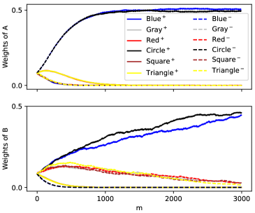
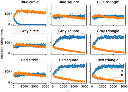
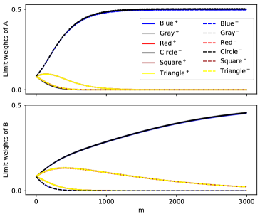
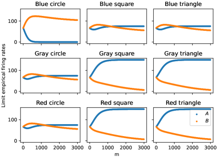
Figure 2: Numerical results with $M=2997$, $\delta t=2$ms, $\lambda=100$Hz and $\nu=150$Hz. Each kind of object is presented alternately. On the top, results for $T=2$s, which corresponds to $N=1000$ time steps. On the bottom, results for the limit parameters (i.e., when $N$ goes to the infinite). On the top (resp. bottom) left, evolution of synaptic weights (resp. limit synaptic weights) of neurons $A$ and $B$ with time. On the top (resp. bottom) right, evolution of the empirical firing rates (resp. limit empirical firing rates) of neurons $A$ and $B$ through time for each kind of object.

The classes are $A=\{{\color[rgb]{0,0,1}\Box},{\color[rgb]{0,0,1}\triangle},{\color[rgb]{.5,.5,.5}\bigcirc},{\color[rgb]{.5,.5,.5}\Box},{\color[rgb]{.5,.5,.5}\triangle},{\color[rgb]{1,0,0}\bigcirc},{\color[rgb]{1,0,0}\Box},{\color[rgb]{1,0,0}\triangle}\}$ and $B=\{{\color[rgb]{0,0,1}\bigcirc}\}$. We consider large $N$; indeed, the refractory period of a biological neuron, which is the time in which a neuron, after emitting a spike, is unable to spike again, lasts a few milliseconds [4]. We choose $\delta t$ of this order: the presentation of an object to the network lasts $T=2s$ and we take $\delta t=2ms$, which corresponds to $N=1000$ time steps by object. See appendix 0.A for numerical results with not very large $N$.

The numerical results of the network learning phase can be seen in Figure 2, as well as the numerical results of the limit parameters. We can see that for $N=1000$, the synaptic weights and empirical firing rates are very close to the limit ones. Here, the parameters $\lambda$ and $\nu$ are chosen so that conditions  (10) and  (11) are satisfied. The object of class $B$ is $\color[rgb]{0,0,1}\bigcirc$, and we can see that the synaptic weights of neurons $A$ and $B$ converge as expected to the pair $(\tilde{q}^{A},\tilde{q}^{B})$ such that $\tilde{q}^{A}$ distributes the weight uniformly over neurons blue^- and circle^- and $\tilde{q}^{B}$ distributes the weight uniformly over neurons blue⁺ and circle⁺.

Looking at the empirical firing rates per object, we see that very quickly, neuron $B$ spikes more than neuron $A$ when presented ${\color[rgb]{0,0,1}\bigcirc}$ and neuron $A$ spikes more than neuron $B$ when presented ${\color[rgb]{.5,.5,.5}\Box},{\color[rgb]{.5,.5,.5}\triangle},{\color[rgb]{1,0,0}\Box},{\color[rgb]{1,0,0}\triangle}$, which are the objects with no features in common with ${\color[rgb]{0,0,1}\bigcirc}$. Thus, the network correctly classifies these objects very quickly. However, when objects with a feature in common with ${\color[rgb]{0,0,1}\bigcirc}$ are presented, for a while neuron $B$ spikes more than neuron $A$, so the network classifies the objects into the wrong class. Then the empirical firing rate of neuron $B$ decreases and neuron $A$ emits more spikes, so the network eventually classifies these objects correctly as well.

4.3 Comparison with Component-Cue

We can compare our algorithm to the original Component-Cue algorithm, for which there is no theoretical guarantee nor a spiking neuronal network interpretation. The results can be seen in Figure 3. We see that Component-Cue is making fewer mistakes at the beginning of the learning but that EWAK is in the end making less mistakes than Component-Cue. Note that the choice of the parameters in Component-Cue is tricky, and that the behavior of the algorithm (learning or not) highly depends on this choice (see details in [18]).

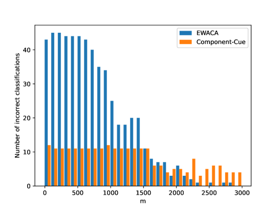
Figure 3: Comparison between EWAK and the exponential version of the Component-Cue model. This is the histogram of incorrect classifications for every $100$ objects for both models, for the objects and classes used in section 4.2. The parameters used for EWAK are the same as in section 4.2. For the Component-Cue model, the parameters are $\lambda_{w}=0.005$ for the learning rate and $\phi=10$ for the parameter of the softmax function used in the model.

5 Conclusion

In this paper, we introduced a Hawkes network that provably learns to classify objects thanks to a local learning rule inspired by an expert aggregation method. This learning rule led to an algorithm (EWAK) allowing us to prove a neuronal discrepancy result on the firing rate and an oracle inequality on the class discrepancy. A promising – but ambitious – line of research is to understand if such local rules can be generalized for Hawkes network with one, or more, hidden layers.

This is the appendix for “Provable local learning rule by expert aggregation for a Hawkes network”. Appendix 0.A provides numerical results in the case where $N$ is not large, and Appendix 0.B-0.F provide the proofs of our results.

Appendix 0.A Numerical results when $N$ is not large enough

The numerical results of the network learning phase with $N=50$ can be seen in Figure 4. The other parameters are the same as in Figure 2. First, we can see that the empirical firing rates are much more scattered than with $N=1000$ (Figure 2). Indeed, with this value of $N$, their variance is significant. Besides, the evolution of the weights is much less regular, and around $m=2200$ the weight $w_{\text{Gray}^{-}\to A}^{m}$ jumps from almost $0$ to almost $1$. This is because before the jump, ${w_{\text{Gray}^{-}\to A}^{m}}^{-1}$ is very large compared to $N$ and as soon as Gray^- is chosen as a neighbour (Step 8 of Algorithm 1), its credit is significantly increased (see  (4)). This provokes major disturbances in the empirical firing rate of neuron $A$. In a sense, it resets its learning process because every weight is put at $0$ except $w_{\text{Gray}^{-}\to A}^{m}$ which is put at $1$; these are not the initial weight values, but these are values far from the weight limits towards which they should tend, i.e., $\frac{1}{2}$ for $w_{\text{Blue}^{-}\to A}^{m}$ and $w_{\text{Circle}^{-}\to A}^{m}$ and $0$ for the others, and which they were close to just before the jump.

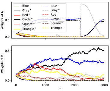
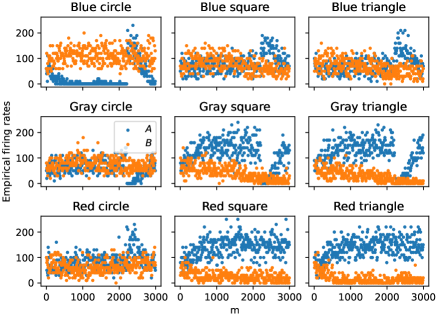
Figure 4: Numerical results with $M=2997$, $\lambda=100$Hz, $\nu=150$Hz, $\delta t=2$ms and $T=0.1$s which corresponds to $N=50$. Each kind of object is presented alternately. On the left, evolution of synaptic weights of neurons $A$ and $B$ with time. On the right, evolution of the empirical firing rates of neurons $A$ and $B$ through time for each kind of object.

Appendix 0.B Proof of proposition 1

Let $(\Omega,\mathcal{F},\mathbb{P})$ be a probability space. Let $\omega\in\Omega$, $m\leq M$. The weights $w_{i\xrightarrow{}j}^{m}(\omega)$ are updated with EWA algorithm using the losses $(-c_{i,m}^{j}(\omega))_{i\in I_{j}}$. The losses take value in $[-G_{M}^{j}(\omega),H_{M}^{j}(\omega)]$. The regret bound given in [3] holds for losses taking value in $[0,1]$, but a more general demonstration for losses only assumed to be bounded is given in [25], and provides the following bound:

$$R_{M}^{j}(\omega)\leq\frac{\ln(\lvert I_{j}\rvert)}{\eta_{M}^{j}}+\eta_{M}^{j}\frac{(H_{M}(\omega)+G_{M}(\omega))^{2}}{8}M.$$

By replacing $\eta_{M}^{j}$ by its value, we get

$$\frac{R_{M}^{j}(\omega)}{M\delta t}\leq\frac{1}{\delta t}\sqrt{\frac{\ln(\lvert I_{j}\rvert)}{8M}}\Big{(}K^{j}+\frac{(G_{M}^{j}(\omega)+H_{M}^{j}(\omega))^{2}}{K^{j}}\Big{)}.$$

It is true for every $\omega$ so almost surely, we have

$$\frac{R_{M}^{j}}{M\delta t}\leq\frac{1}{\delta t}\sqrt{\frac{\ln(\lvert I_{j}\rvert)}{8M}}\Big{(}K^{j}+\frac{(G_{M}^{j}+H_{M}^{j})^{2}}{K^{j}}\Big{)}.$$

Appendix 0.C Proof of Theorem 3.2

We want to bound from below $\frac{1}{\lvert J\rvert}\sum_{j\in J}\Gamma^{j}_{M}(W)$. We have almost surely

$$\frac{1}{\lvert J\rvert}\sum_{j\in J}\Gamma^{j}_{M}(W)=\frac{1}{\lvert J\rvert}\sum_{j\in J}F_{M}^{j,j}(W^{j})-\frac{1}{\lvert J\rvert}\sum_{j\in J}\frac{1}{\lvert J\rvert-1}\sum_{j^{\prime}\neq j}F_{M}^{j^{\prime},j}(W^{j^{\prime}})$$

Let us exchange the name of the indexes $j$ and $j^{\prime}$ in the second term.

$$\frac{1}{\lvert J\rvert}\sum_{j\in J}\Gamma^{j}_{M}(W)= \frac{1}{\lvert J\rvert}\sum_{j\in J}F_{M}^{j,j}(W^{j})-\frac{1}{\lvert J\rvert}\sum_{j^{\prime}\in J}\frac{1}{\lvert J\rvert-1}\sum_{j\neq j^{\prime}}F_{M}^{j,j^{\prime}}(W^{j})$$

Let us exchange the sums in the second term.

$$\frac{1}{\lvert J\rvert}\sum_{j\in J}\Gamma^{j}_{M}(W)= \frac{1}{\lvert J\rvert}\sum_{j\in J}F_{M}^{j,j}(W^{j})-\frac{1}{\lvert J\rvert}\sum_{j\in J}\frac{1}{\lvert J\rvert-1}\sum_{j^{\prime}\neq j}F_{M}^{j,j^{\prime}}(W^{j})$$

$$= \frac{1}{\lvert J\rvert}\sum_{j\in J}\Big{(}F_{M}^{j,j}(W^{j})-\frac{1}{\lvert J\rvert-1}\sum_{j^{\prime}\neq j}F_{M}^{j,j^{\prime}}(W^{j})\Big{)}$$

$$= \frac{1}{\lvert J\rvert}\sum_{j\in J}D_{M}^{j}(W_{j})$$

$$\geq \frac{1}{\lvert J\rvert}\sum_{j\in J}\Big{(}D_{M}^{j}(Q^{j})-E_{\text{reg}}^{j}(M)\Big{)}$$

thanks to inequality (7).

$$\frac{1}{\lvert J\rvert}\sum_{j\in J}\Gamma^{j}_{M}(W)\geq \frac{1}{\lvert J\rvert}\sum_{j\in J}\Big{(}F_{M}^{j,j}(Q^{j})-\frac{1}{\lvert J\rvert-1}\sum_{j^{\prime}\neq j}F_{M}^{j,j^{\prime}}(Q^{j})\Big{)}-\frac{1}{\lvert J\rvert}\sum_{j\in J}E_{\text{reg}}^{j}(M)$$

$$= \frac{1}{\lvert J\rvert}\sum_{j\in J}F_{M}^{j,j}(Q^{j})-\frac{1}{\lvert J\rvert}\sum_{j\in J}\frac{1}{\lvert J\rvert-1}\sum_{j^{\prime}\neq j}F_{M}^{j,j^{\prime}}(Q^{j})-\frac{1}{\lvert J\rvert}\sum_{j\in J}E_{\text{reg}}^{j}(M)$$

Let us exchange the sums in the second term.

$$\frac{1}{\lvert J\rvert}\sum_{j\in J}\Gamma^{j}_{M}(W)\geq \frac{1}{\lvert J\rvert}\sum_{j\in J}F_{M}^{j,j}(Q^{j})-\frac{1}{\lvert J\rvert}\sum_{j^{\prime}\in J}\frac{1}{\lvert J\rvert-1}\sum_{j\neq j^{\prime}}F_{M}^{j,j^{\prime}}(Q^{j})-\frac{1}{\lvert J\rvert}\sum_{j\in J}E_{\text{reg}}^{j}(M)$$

Let us exchange the name of the indexes $j$ and $j^{\prime}$ in the second term.

$$\frac{1}{\lvert J\rvert}\sum_{j\in J}\Gamma^{j}_{M}(W)\geq \frac{1}{\lvert J\rvert}\sum_{j\in J}F_{M}^{j,j}(Q^{j})-\frac{1}{\lvert J\rvert}\sum_{j\in J}\frac{1}{\lvert J\rvert-1}\sum_{j^{\prime}\neq j}F_{M}^{j^{\prime},j}(Q^{j^{\prime}})-\frac{1}{\lvert J\rvert}\sum_{j\in J}E_{\text{reg}}^{j}(M)$$

$$= \frac{1}{\lvert J\rvert}\sum_{j\in J}\Big{(}F_{M}^{j,j}(Q^{j})-\frac{1}{\lvert J\rvert-1}\sum_{j^{\prime}\neq j}F_{M}^{j^{\prime},j}(Q^{j^{\prime}})\Big{)}-\frac{1}{\lvert J\rvert}\sum_{j\in J}E_{\text{reg}}^{j}(M)$$

$$= \frac{1}{\lvert J\rvert}\sum_{j\in J}\Gamma^{j}_{M}(Q)-\frac{1}{\lvert J\rvert}\sum_{j\in J}E_{\text{reg}}^{j}(M)$$

Let

• $\overline{f}_{m}^{j}(q^{j}):=\sum\limits_{i\in I_{j}}q_{i}^{j}\dfrac{p_{i,m}}{\delta t}$. This is the exact firing rate of neuron $j$ with synaptic weights $q^{j}$ when presented with the $m^{th}$ object.

• $\overline{F}_{M}^{j^{\prime},j}(Q^{j^{\prime}}):=\dfrac{1}{j_{M}}\sum\limits_{m,\text{ }o(m)\in j}\overline{f}_{m}^{j^{\prime}}(q^{j^{\prime}})$. It is the average firing rate of neuron $j^{\prime}$ with stationary synaptic weights $q^{j^{\prime}}$ during the presentation of objects in class $j$.

• $\dfrac{1}{\lvert J\rvert}\sum_{j\in J}\overline{\Gamma}^{j}_{M}(Q):=\dfrac{1}{\lvert J\rvert}\sum\limits_{j\in J}\Big{(}\overline{F}_{M}^{j,j}(Q^{j})-\dfrac{1}{\lvert J\rvert-1}\sum\limits_{j^{\prime}\neq j}\overline{F}_{M}^{j^{\prime},j}(Q^{j^{\prime}})\Big{)}$ is the corresponding average class discrepancy.

The family $q$ is a feasible weight family, so for all $j\in J$, $j^{\prime}\neq j$, $m\leq M$ such that $o(m)\in j$,

$$\overline{f}_{m}^{j}(q^{j})\geq\overline{f}_{m}^{j^{\prime}}(q^{j^{\prime}})+\Delta(q).$$

so

$$\overline{F}_{M}^{j,j}(Q^{j})\geq\overline{F}_{M}^{j^{\prime},j}(Q^{j^{\prime}})+\Delta(q)$$

and

$$\frac{1}{\lvert J\rvert}\sum_{j\in J}\overline{\Gamma}^{j}_{M}(Q)\geq\Delta(q).$$

We would like to prove that $\Gamma^{j}_{M}(Q)$ is close to $\overline{\Gamma}^{j}_{M}(Q)$ with high probability, and give an explicit expression of the error term. For this purpose, we need the following result.

Theorem 0.C.1

Let $\alpha>0$. Then for all synaptic weights $q=(q^{j})_{j\in J}$, we have

$$\mathbb{P}\Big{(}\forall m\leq M,j\in J,j^{\prime}\in J,|F_{M}^{j^{\prime},j}(Q^{j^{\prime}})-\overline{F}_{M}^{j^{\prime},j}(Q^{j^{\prime}})|\leq e_{\text{approx}}^{j^{\prime},j}\Big{)}\geq 1-\alpha$$

Proof

First, let us rewrite $N_{i,m}^{j}$ the following way for $m\leq M$, $j\in J$, $i\in I_{j}$:

$$N_{i,m}^{j}=\sum\limits_{t=1}^{N}\mathbf{1}_{\{\sum\limits_{l=1}^{i-1}w_{l\xrightarrow{}j}^{m}<U_{m,t}^{j}\leq\sum\limits_{l=1}^{i}w_{l\xrightarrow{}j}^{m}\}}X_{i,m,t-1}$$ (12)

where the random variables $U_{m,k}^{j}$ are i.i.d following a uniform distribution on $[0,1]$, independent from the neurons activity. The random variable

$$\mathbf{1}_{\{\sum\limits_{l=1}^{i-1}w_{l\xrightarrow{}j}^{m}<U_{m,t}^{j}\leq\sum\limits_{l=1}^{i}w_{l\xrightarrow{}j}^{m}\}}$$

corresponds to the choice of a presynaptic neuron in Kalikow decomposition at time $t$ during the presentation of the $m^{th}$ object. We remind that the sequence $(X_{i,m,t})_{0\leq t\leq N}$ corresponds to the activity of input neuron $i$ when presented the $m^{th}$ object: it is a sequence of i.i.d random variables following a Bernoulli distribution. We suppose that for each object, input neurons start to spike at time $t=0$ (it corresponds to $X_{i,m,0}$), and output neurons at time $t=1$.

Knowing the variables $w_{m}^{j}=(w_{l\xrightarrow{}j}^{m})_{l\in I_{j}}$, the quantity $N_{i,m}^{j}$ is the sum of independent random variables bounded by $1$. Then, thanks to Bernstein inequality, for all $x\geq 0$ we have

$$\mathbb{P}\Big{(}|N_{i,m}^{j}-\mathbb{E}[N_{i,m}^{j}|w_{m}^{j}]|\geq\sqrt{2\text{Var}(N_{i,m}^{j}|w_{m}^{j})x}+\frac{x}{3}\mid w_{m}^{j}\Big{)}\leq 2e^{-x}.$$

Besides, knowing $w_{m}^{j}$, the variable $N_{i,m}^{j}$ follows a binomial distribution with parameters $N$ and $p_{i,m}w_{i\xrightarrow{}j}^{m}$. Hence,

$$\mathbb{E}[N_{i,m}^{j}|w_{m}^{j}] =Np_{i,m}w_{i\xrightarrow{}j}^{m}$$

$$\text{Var}(N_{i,m}^{j}|w_{m}^{j}) =Np_{i,m}w_{i\xrightarrow{}j}^{m}(1-p_{i,m}w_{i\xrightarrow{}j}^{m})\leq Np_{i,m}w_{i\xrightarrow{}j}^{m}.$$

Hence,

$$\mathbb{P}\Big{(}|N_{i,m}^{j}-Np_{i,m}w_{i\xrightarrow{}j}^{m}|\geq\sqrt{2Np_{i,m}w_{i\xrightarrow{}j}^{m}x}+\frac{x}{3}\Big{)}\leq 2e^{-x}.$$

Let us choose $x=x_{j}$ such that $2e^{-x_{j}}=\dfrac{\alpha}{M\lvert J\rvert\lvert I_{j}\rvert}$, i.e., $x_{j}=\ln\Big{(}\frac{2M\lvert J\rvert\lvert I_{j}\rvert}{\alpha}\Big{)}$. Let $D^{c}$ be the event

$$D^{c}=\Big{\{}\exists m\leq M,j\in J,i\in I_{j},|N_{i,m}^{j}-Np_{i,m}w_{i\xrightarrow{}j}^{m}|\geq\sqrt{2Np_{i,m}w_{i\xrightarrow{}j}^{m}x_{j}}+\frac{1}{3}x_{j}\Big{\}}.$$

Then,

$$\mathbb{P}(D^{c}) =\mathbb{P}\Big{(}\bigcup_{\begin{subarray}{l}1\leq m\leq M\\ j\in J,\text{ }i\in I_{j}\end{subarray}}\Big{\{}|N_{i,m}^{j}-Np_{i,m}w_{i\xrightarrow{}j}^{m}|\geq\sqrt{2Np_{i,m}w_{i\xrightarrow{}j}^{m}x_{j}}+\frac{1}{3}x_{j}\Big{\}}\Big{)}$$

$$\leq\sum_{\begin{subarray}{l}1\leq m\leq M\\ j\in J,\text{ }i\in I_{j}\end{subarray}}\mathbb{P}\Big{(}|N_{i,m}^{j}-Np_{i,m}w_{i\xrightarrow{}j}^{m}|\geq\sqrt{2Np_{i,m}w_{i\xrightarrow{}j}^{m}x_{j}}+\frac{1}{3}x_{j}\Big{)}$$

$$\leq\sum_{\begin{subarray}{l}1\leq m\leq M\\ j\in J,\text{ }i\in I_{j}\end{subarray}}\frac{\alpha}{M\lvert J\rvert\lvert I_{j}\rvert}$$

$$=\alpha$$

Hence $\mathbb{P}(D)\geq 1-\alpha$. Let $m\leq M$, $j\in J$, $j^{\prime}\in J$ not necessarily distinct from $j$. On $D$, we have

$$|F_{M}^{j^{\prime},j}(Q^{j^{\prime}})-\overline{F}_{M}^{j^{\prime},j}(Q^{j^{\prime}})|= \left\lvert\dfrac{1}{j_{M}}\sum\limits_{m,\text{ }o(m)\in j}(f_{m}^{j^{\prime}}(q^{j^{\prime}})-\overline{f}_{m}^{j^{\prime}}(q^{j^{\prime}}))\right\rvert$$

$$\leq \dfrac{1}{j_{M}}\sum\limits_{m,\text{ }o(m)\in j}\sum_{i\in I_{j^{\prime}}}\frac{q_{i}^{j^{\prime}}}{\delta t}\left\lvert\frac{N_{i,m}^{j^{\prime}}}{Nw_{i\xrightarrow{}j^{\prime}}^{m}}-p_{i,m}\right\rvert$$

$$\leq \dfrac{1}{j_{M}}\sum\limits_{m,\text{ }o(m)\in j}\sum_{i\in I_{j^{\prime}}}\frac{q_{i}^{j^{\prime}}}{\delta t}\left[\sqrt{\frac{2p_{i,m}}{Nw_{i\xrightarrow{}j^{\prime}}^{m}}x_{j^{\prime}}}+\frac{1}{3Nw_{i\xrightarrow{}j}^{m}}x_{j^{\prime}}\right]$$

$$= e_{\text{approx}}^{j^{\prime},j}$$

Hence

$$D\subset\Big{\{}\forall m\leq M,j\in J,j^{\prime}\in J,|F_{M}^{j^{\prime},j}(q^{j^{\prime}})-\overline{F}_{M}^{j^{\prime},j}(q^{j^{\prime}})|\leq e_{\text{approx}}^{j^{\prime},j}\Big{\}}$$

so

$$\mathbb{P}\Big{(}\forall m\leq M,j\in J,j^{\prime}\in J,|F_{M}^{j^{\prime},j}(Q^{j^{\prime}})-\overline{F}_{M}^{j^{\prime},j}(Q^{j^{\prime}})|\leq e_{\text{approx}}^{j^{\prime},j}\Big{)}\geq 1-\alpha.$$

Then with probability $1-\alpha$,

$$\frac{1}{\lvert J\rvert}\sum_{j\in J}\Gamma^{j}_{M}(W)\geq\frac{1}{\lvert J\rvert}\sum_{j\in J}\overline{\Gamma}^{j}_{M}(Q)-\frac{1}{\lvert J\rvert}\sum_{j\in J}\Big{(}e_{\text{approx}}^{j,j}+\frac{1}{\lvert J\rvert-1}\sum_{j^{\prime}\neq j}e_{\text{approx}}^{j^{\prime},j}\Big{)}-\frac{1}{\lvert J\rvert}\sum_{j\in J}E_{\text{reg}}^{j}(M)$$

Besides, by exchanging the two sums and the name of the indexes $j$ and $j^{\prime}$, we have

$$\frac{1}{\lvert J\rvert}\sum_{j\in J}\frac{1}{\lvert J\rvert-1}\sum_{j^{\prime}\neq j}e_{\text{approx}}^{j^{\prime},j}=\frac{1}{\lvert J\rvert}\sum_{j\in J}\frac{1}{\lvert J\rvert-1}\sum_{j^{\prime}\neq j}e_{\text{approx}}^{j,j^{\prime}}$$

i.e.,

$$\frac{1}{\lvert J\rvert}\sum_{j\in J}\Gamma^{j}_{M}(W)\geq\frac{1}{\lvert J\rvert}\sum_{j\in J}\overline{\Gamma}^{j}_{M}(Q)-E_{\text{tot}}(M,q,\alpha).$$

Appendix 0.D Proof of Theorem 3.3 and choice of $K^{j}$ in Proposition 1

0.D.1 Proof of Theorem 3.3

We recall that

$$\overline{c}_{i,m}^{j}=\left\{\begin{array}[]{ll}p_{i,m}\times\frac{M}{j_{M}}&\text{if }o(m)\in j\\ -p_{i,m}\times\frac{1}{\lvert J\rvert-1}\times\frac{M}{j_{M}^{{}^{\prime}}}&\text{if }o(m)\in j^{\prime}\neq j,\end{array}\right.\overline{C}_{i,m}^{j}=\sum\limits_{m^{\prime}=1}^{m}\overline{c}_{i,m^{\prime}}^{j}\text{ and }\overline{w}_{i\xrightarrow{}j}^{m}=\dfrac{\text{exp}(\eta_{M}^{j}\overline{C}_{i,m-1}^{j})}{\sum\limits_{l\in I_{j}}\text{exp}(\eta_{M}^{j}\overline{C}_{l,m-1}^{j})}.$$

To clarify the dependency on $N$ of the network parameters, we will use the following notations: $w_{i\xrightarrow{}j}^{m,N}$, $c_{i,m}^{j,N}$, $C_{i,m}^{j,N}$ and $N_{i,m}^{j,N}$.

Let us prove by induction that for all $m\geq 1$, $j\in J$, $i\in I_{j}$, we have

$$w_{i\xrightarrow{}j}^{m,N}\xrightarrow[N\xrightarrow{}\infty]{\mathbb{P}}\overline{w}_{i\xrightarrow{}j}^{m},\quad c_{i,m}^{j,N}\xrightarrow[N\xrightarrow{}\infty]{\mathbb{P}}\overline{c}_{i,m}^{j}\quad\text{ and }\quad C_{i,m}^{j,N}\xrightarrow[N\xrightarrow{}\infty]{\mathbb{P}}\overline{C}_{i,m}^{j}.$$

Case $m=1$. According to the weights definition, $w_{i\xrightarrow{}j}^{1,N}=\dfrac{1}{\lvert I_{j}\rvert}$ and $\overline{w}_{i\xrightarrow{}j}^{1}=\dfrac{1}{\lvert I_{j}\rvert}$. According to  (12), we have

$$\frac{N_{i,1}^{j}}{N} =\frac{1}{N}\sum\limits_{t=1}^{N}\mathbf{1}_{\{\sum\limits_{l=1}^{i-1}w_{l\xrightarrow{}j}^{1,N}<U_{1,t}^{j}\leq\sum\limits_{l=1}^{i}w_{l\xrightarrow{}j}^{1,N}\}}X_{i,1,t-1}$$

$$=\frac{1}{N}\sum\limits_{t=1}^{N}\mathbf{1}_{\{\sum\limits_{l=1}^{i-1}\overline{w}_{l\xrightarrow{}j}^{1}<U_{1,t}^{j}\leq\sum\limits_{l=1}^{i}\overline{w}_{l\xrightarrow{}j}^{1}\}}X_{i,1,t-1}$$

The random variables in the sum are i.i.d. They follow a Bernoulli distribution of parameter $\overline{w}_{i\xrightarrow{}j}^{1}p_{i,1}$ (thanks to the indendence of $X_{i,1,t-1}$ with $U_{1,t}^{j}$). According to the law of large numbers,

$$\frac{N_{i,1}^{j}}{N}\xrightarrow[N\xrightarrow{}\infty]{\mathbb{P}}\overline{w}_{i\xrightarrow{}j}^{1}p_{i,1}$$

i.e.,

$$c_{i,1}^{j,N}\xrightarrow[N\xrightarrow{}\infty]{\mathbb{P}}\overline{c}_{i,1}^{j}.$$

Moreover, we have $C_{i,1}^{j,N}=c_{i,1}^{j,N}\xrightarrow[N\xrightarrow{}\infty]{\mathbb{P}}\overline{c}_{i,1}^{j}=\overline{C}_{i,1}^{j}$.

Case $m>1$. Suppose the convergences are true for $m-1$. We have the convergence in probability of

$$w_{i\xrightarrow{}j}^{m,N}=\dfrac{e^{\eta_{M}^{j}C_{i,m-1}^{j,N}}}{\sum\limits\limits_{l\in I_{j}}e^{\eta_{M}^{j}C_{l,m-1}^{j,N}}}\xrightarrow[N\xrightarrow{}\infty]{\mathbb{P}}\dfrac{e^{\eta_{M}^{j}\overline{C}_{i,m-1}^{j,N}}}{\sum\limits\limits_{l\in I_{j}}e^{\eta_{M}^{j}\overline{C}_{l,m-1}^{j,N}}}=\overline{w}_{i\xrightarrow{}j}^{m}$$

Let $\varepsilon>0$. According to  (12), knowing the weight $w_{i\xrightarrow{}j}^{m,N}$, the random variable $N_{i,m}^{j,N}$ follows a binomial distribution with parameters $N$ and $w_{i\xrightarrow{}j}^{m,N}p_{i,m}$ (because the variables $X_{i,m,t}$ are independent from $w_{i\xrightarrow{}j}^{m,N}$). Then

$$\mathbb{E}\Big{[}\frac{N_{i,m}^{j,N}}{N}\mid w_{i\xrightarrow{}j}^{m,N}\Big{]}=p_{i,m}w_{i\xrightarrow{}j}^{m,N}\quad\text{and}\quad\text{Var}\Big{[}\frac{N_{i,m}^{j,N}}{N}\mid w_{i\xrightarrow{}j}^{m,N}\Big{]}=\frac{w_{i\xrightarrow{}j}^{m,N}p_{i,m}(1-w_{i\xrightarrow{}j}^{m,N}p_{i,m})}{N}.$$

Then, according to to Bienaymé–Chebyshev inequality,

$$\mathbb{P}\Big{(}|\frac{N_{i,m}^{j,N}}{N}-w_{i\xrightarrow{}j}^{m,N}p_{i,m}|\geq\varepsilon\mid w_{i\xrightarrow{}j}^{m,N}\Big{)} \leq\frac{w_{i\xrightarrow{}j}^{m,N}p_{i,m}(1-w_{i\xrightarrow{}j}^{m,N}p_{i,m})}{N\varepsilon^{2}}\leq\frac{1}{N\varepsilon^{2}}.$$

Hence,

$$\mathbb{P}\Big{(}|\frac{N_{i,m}^{j,N}}{N}-w_{i\xrightarrow{}j}^{m,N}p_{i,m}|\geq\varepsilon\Big{)}\leq\frac{1}{N\varepsilon^{2}}\xrightarrow[N\xrightarrow{}\infty]{}0.$$

This means that

$$\frac{N_{i,m}^{j,N}}{N}-w_{i\xrightarrow{}j}^{m,N}p_{i,m}\xrightarrow[N\xrightarrow{}\infty]{\mathbb{P}}0.$$

Thus,

$$\frac{N_{i,m}^{j,N}}{Nw_{i\xrightarrow{}j}^{m,N}}\xrightarrow[N\xrightarrow{}\infty]{\mathbb{P}}p_{i,m}.$$ (13)

Therefore,

$$c_{i,m}^{j,N}\xrightarrow[N\xrightarrow{}\infty]{\mathbb{P}}\overline{c}_{i,m}^{j,N}.$$

Finally, $C_{i,m}^{j,N}=C_{i,m-1}^{j,N}+c_{i,m}^{j,N}\xrightarrow[N\xrightarrow{}\infty]{\mathbb{P}}\overline{C}_{i,m-1}^{j}+\overline{c}_{i,m}^{j}=\overline{C}_{i,m}$.

0.D.2 Details about the choice of $K^{j}$ in Proposition 1

Let

$$\overline{G}_{M}^{j}=\max\limits_{\begin{subarray}{l}1\leq m\leq M\\ i\in I_{j}\end{subarray}}\overline{c}_{i,m}^{j}\quad\text{and}\quad\overline{H}_{M}^{j}:=\max\limits_{\begin{subarray}{l}1\leq m\leq M\\ i\in I_{j}\end{subarray}}-\overline{c}_{i,m}^{j}.$$

Then

$$G_{M}^{j}=\max\limits_{\begin{subarray}{l}1\leq m\leq M\\ i\in I_{j}\end{subarray}}c_{i,m}^{j}\xrightarrow[N\xrightarrow{}\infty]{\mathbb{P}}\max\limits_{\begin{subarray}{l}1\leq m\leq M\\ i\in I_{j}\end{subarray}}\overline{c}_{i,m}^{j}=\overline{G}_{M}^{j}$$

and

$$H_{M}^{j}=\max\limits_{\begin{subarray}{l}1\leq m\leq M\\ i\in I_{j}\end{subarray}}-c_{i,m}^{j}\xrightarrow[N\xrightarrow{}\infty]{\mathbb{P}}\max\limits_{\begin{subarray}{l}1\leq m\leq M\\ i\in I_{j}\end{subarray}}-\overline{c}_{i,m}^{j}=\overline{H}_{M}^{j}.$$

Suppose Assumptions 3.1 and 3.4 hold. Then for every $j\in J$, $\dfrac{M}{j_{M}}=\dfrac{\lvert\mathcal{O}\rvert}{n_{j}}$. Let

$$K:=\Big{(}1+\frac{1}{\lvert J\rvert-1}\Big{)}\max_{j\in J}\Big{\{}\dfrac{\lvert\mathcal{O}\rvert}{n_{j}}\times\max_{i\in I_{j},o\in j}p_{i,o}\Big{\}}.$$

Then

$$\overline{G}_{M}^{j}+\overline{H}_{M}^{j}\leq K$$

and choosing $K^{j}=K$ is a sensible choice to minimize the bound of Proposition 1.

Appendix 0.E Proof of Theorem 3.5,  (9) and Corollary 1

0.E.1 Proof of Theorem 3.5

First, let’s prove that for all $m\geq 1$, for all $j\in J$ and $i\in I_{j}$

$$\overline{C}_{i,M}^{j}=d_{i}^{j}\delta tM.$$ (14)

Indeed,

$$\overline{C}_{i,M}^{j} =\sum_{m=1}^{M}\overline{c}_{i,m}^{j}$$

$$=\sum_{m,\text{ }o(m)\in j}\frac{M}{j_{M}}\times p_{i,m}-\sum_{j^{\prime}\neq j}\sum_{m,\text{ }o(m)\in j^{\prime}}\frac{1}{\lvert J\rvert-1}\times\frac{M}{j_{M}^{{}^{\prime}}}\times p_{i,m}$$

$$=M\Big{(}\frac{1}{j_{M}}\sum_{m,\text{ }o(m)\in j}p_{i,m}-\frac{1}{\lvert J\rvert-1}\sum_{j^{\prime}\neq j}\frac{1}{j_{M}^{{}^{\prime}}}\sum_{m,\text{ }o(m)\in j^{\prime}}p_{i,m}\Big{)}$$

$$=M\Big{(}\frac{1}{j_{M}}\sum_{o\in j}\sum_{m,\text{ }o(m)=o}p_{i,o}-\frac{1}{\lvert J\rvert-1}\sum_{j^{\prime}\neq j}\frac{1}{j_{M}^{{}^{\prime}}}\sum_{o\in j^{\prime}}\sum_{m,\text{ }o(m)=o}p_{i,o}\Big{)}$$

Besides, each kind of object is presented the same amount of times, so for all $j\in J$,

$$j_{M}=n_{j}\times\frac{M}{\lvert O\rvert}$$

so we have

$$\overline{C}_{i,M}^{j} =M\Big{(}\frac{1}{n_{j}}\sum_{o\in j}p_{i,o}-\frac{1}{\lvert J\rvert-1}\sum_{j^{\prime}\neq j}\frac{1}{n_{j^{\prime}}}\sum_{o\in j^{\prime}}p_{i,o}\Big{)}$$

$$=d_{i}^{j}\delta tM.$$

Let $d_{\text{max}}^{j}:=\max\limits_{i\in I_{j}}d_{i}^{j}$.

Case $\tilde{I}_{j}=I_{j}$. Then for all $i\in I_{j}$,

$$\overline{w}_{i\xrightarrow{}j}^{M+1}=\dfrac{\exp(\eta_{M}^{j}d_{\text{max}}^{j}\delta tM)}{\sum\limits_{l\in I_{j}}\exp(\eta_{M}^{j}d_{\text{max}}^{j}\delta tM)}=\frac{1}{\lvert I_{j}\rvert}.$$

Case $\tilde{I}_{j}\neq I_{j}$. Then

$$\overline{w}_{i\xrightarrow{}j}^{M+1}=\dfrac{e^{\eta_{M}^{j}Md_{i}^{j}\delta t}}{\sum\limits_{l\in I_{j}}e^{\eta_{M}^{j}Md_{l}^{j}\delta t}}\leq\frac{e^{\eta_{M}^{j}Md_{i}^{j}\delta t}}{\lvert\tilde{I}_{j}\rvert e^{\eta_{M}^{j}Md_{\text{max}}^{j}\delta t}}=\frac{1}{\lvert\tilde{I}_{j}\rvert}e^{-\eta_{M}^{j}M(d_{\text{max}}^{j}-d_{i}^{j})\delta t}.$$

Thus

$$0\leq\overline{w}_{i\xrightarrow{}j}^{M+1}\leq\frac{1}{\lvert\tilde{I}_{j}\rvert}e^{-\eta_{M}^{j}M(d_{\text{max}}^{j}-d_{i}^{j})\delta t}.$$ (15)

Let $i\in\tilde{I}_{j}$, $d_{\text{max bis}}^{j}:=\max\limits_{i\in I_{j}\setminus\tilde{I}_{j}}d_{i}^{j}$.

$$\overline{w}_{i\xrightarrow{}j}^{M+1} =\dfrac{e^{\eta_{M}^{j}Md_{i}^{j}\delta t}}{\sum\limits_{l\in I_{j}}e^{\eta_{M}^{j}Md_{l}^{j}\delta t}}$$

$$\geq\frac{e^{\eta_{M}^{j}Md_{\text{max}}^{j}\delta t}}{\lvert\tilde{I}_{j}\rvert e^{\eta_{M}^{j}Md_{\text{max}}^{j}\delta t}+(\lvert I_{j}\rvert-\lvert\tilde{I}_{j}\rvert)e^{\eta_{M}^{j}Md_{\text{max bis}}^{j}\delta t}}$$

$$=\frac{1}{\lvert\tilde{I}_{j}\rvert}\frac{1}{1+\frac{\lvert I_{j}\rvert-\lvert\tilde{I}_{j}\rvert}{\lvert\tilde{I}_{j}\rvert}e^{-\eta_{M}^{j}\gamma_{j}M\delta t}}$$

$$\geq\frac{1}{\lvert\tilde{I}_{j}\rvert}\Big{(}1-\frac{\lvert I_{j}\rvert-\lvert\tilde{I}_{j}\rvert}{\lvert\tilde{I}_{j}\rvert}e^{-\eta_{M}^{j}\gamma_{j}M\delta t}\Big{)}$$

$$=\frac{1}{\lvert\tilde{I}_{j}\rvert}-\frac{\lvert I_{j}\rvert-\lvert\tilde{I}_{j}\rvert}{\lvert\tilde{I}_{j}\rvert^{2}}e^{-\eta_{M}^{j}\gamma_{j}M\delta t},$$

and thanks to  (15),

$$\overline{w}_{i\xrightarrow{}j}^{M+1}\leq\dfrac{1}{\lvert\tilde{I}_{j}\rvert}.$$

Thus

$$\frac{1}{\lvert\tilde{I}_{j}\rvert}-\frac{\lvert I_{j}\rvert-\lvert\tilde{I}_{j}\rvert}{\lvert\tilde{I}_{j}\rvert^{2}}e^{-\eta_{M}^{j}\gamma_{j}M\delta t}\leq\overline{w}_{i\xrightarrow{}j}^{M+1}\leq\frac{1}{\lvert\tilde{I}_{j}\rvert}.$$

Let $i\in I\setminus\tilde{I}_{j}$. Then  (15) tells us that

$$0\leq\overline{w}_{i\xrightarrow{}j}^{M+1}\leq\frac{1}{\lvert\tilde{I}_{j}\rvert}e^{-\eta_{M}^{j}M\gamma_{j}\delta t}.$$

In particular, with $\eta_{M}^{j}=\dfrac{1}{K^{j}}\sqrt{\dfrac{8ln(\lvert I_{j}\rvert)}{M}}$, for all $i\in I_{j}$

$$\lvert\overline{w}_{i\to j}^{M+1}-\tilde{q}_{i}^{j}\rvert\leq\overline{E}^{j}(M)$$

0.E.2 Proof of  (9)

Let us recall that

$$D_{M}^{j}(\tilde{Q}^{j}) =F_{M}^{j,j}(\tilde{Q}^{j})-\dfrac{1}{\lvert J\rvert-1}\sum\limits_{j^{\prime}\neq j}F_{M}^{j,j^{\prime}}(\tilde{Q}^{j})$$

$$=\dfrac{1}{j_{M}}\sum\limits_{m,\text{ }o(m)\in j}f_{m}^{j}(\tilde{q}^{j})-\frac{1}{\lvert J\rvert-1}\sum_{j^{\prime}\neq j}\dfrac{1}{j_{M}^{{}^{\prime}}}\sum\limits_{m,\text{ }o(m)\in j^{\prime}}f_{m}^{j}(\tilde{q}^{j})$$

$$=\dfrac{1}{j_{M}}\sum\limits_{m,\text{ }o(m)\in j}\sum_{i\in I_{j}}\frac{\tilde{q}_{i}^{j}}{\delta t}\frac{N_{i,m}^{j}}{Nw_{i\xrightarrow{}j}^{m}}-\frac{1}{\lvert J\rvert-1}\sum_{j^{\prime}\neq j}\dfrac{1}{j_{M}^{{}^{\prime}}}\sum\limits_{m,\text{ }o(m)\in j^{\prime}}\frac{\tilde{q}_{i}^{j}}{\delta t}\frac{N_{i,m}^{j}}{Nw_{i\xrightarrow{}j}^{m}}$$

Besides, according to  (13),

$$\frac{N_{i,m}^{j}}{Nw_{i\xrightarrow{}j}^{m}}\xrightarrow[N\xrightarrow{}\infty]{\mathbb{P}}p_{i,m}.$$

Let

$$\overline{D}_{M}^{j}(\tilde{Q}^{j}):=\dfrac{1}{j_{M}}\sum\limits_{m,\text{ }o(m)\in j}\sum_{i\in I_{j}}\frac{\tilde{q}_{i}^{j}}{\delta t}p_{i,m}-\frac{1}{\lvert J\rvert-1}\sum_{j^{\prime}\neq j}\dfrac{1}{j_{M}^{{}^{\prime}}}\sum\limits_{m,\text{ }o(m)\in j^{\prime}}\frac{\tilde{q}_{i}^{j}}{\delta t}p_{i,m}.$$

Then

$$D_{M}^{j}(\tilde{Q}^{j})\xrightarrow[N\xrightarrow{}\infty]{\mathbb{P}}\overline{D}_{M}^{j}(\tilde{Q}^{j})$$

and

$$\overline{D}_{M}^{j}(\tilde{Q}^{j}) =\dfrac{1}{j_{M}}\sum_{m,\text{ }o(m)\in j}\overline{f}_{m}^{j}(\tilde{q}^{j})-\frac{1}{\lvert J\rvert-1}\sum_{j^{\prime}\neq j}\dfrac{1}{j_{M}^{{}^{\prime}}}\sum\limits_{m,\text{ }o(m)\in j^{\prime}}\overline{f}_{m}^{j}(\tilde{q}^{j})$$

$$=\dfrac{1}{j_{M}}\sum_{o\in j}\sum_{m,\text{ }o(m)=o}\overline{f}_{o}^{j}(\tilde{q}^{j})-\frac{1}{\lvert J\rvert-1}\sum_{j^{\prime}\neq j}\dfrac{1}{j_{M}^{{}^{\prime}}}\sum_{o\in j^{\prime}}\sum\limits_{m,\text{ }o(m)=o}\overline{f}_{o}^{j}(\tilde{q}^{j})$$

$$=\dfrac{1}{n_{j}}\sum_{o\in j}\overline{f}_{o}^{j}(\tilde{q}^{j})-\frac{1}{\lvert J\rvert-1}\sum_{j^{\prime}\neq j}\dfrac{1}{n_{j^{\prime}}}\sum_{o\in j^{\prime}}\overline{f}_{o}^{j}(\tilde{q}^{j})$$

$$=\dfrac{1}{n_{j}}\sum_{o\in j}\sum_{i\in I_{j}}\tilde{q}_{i}^{j}\frac{p_{i,o}}{\delta t}-\frac{1}{\lvert J\rvert-1}\sum_{j^{\prime}\neq j}\dfrac{1}{n_{j^{\prime}}}\sum_{o\in j^{\prime}}\sum_{i\in I_{j}}\tilde{q}_{i}^{j}\frac{p_{i,o}}{\delta t}$$

$$=\dfrac{1}{n_{j}}\sum_{o\in j}\sum_{i\in\tilde{I}_{j}}\frac{1}{\lvert\tilde{I}_{j}\rvert}\frac{p_{i,o}}{\delta t}-\frac{1}{\lvert J\rvert-1}\sum_{j^{\prime}\neq j}\dfrac{1}{n_{j^{\prime}}}\sum_{o\in j^{\prime}}\sum_{i\in\tilde{I}_{j}}\frac{1}{\lvert\tilde{I}_{j}\rvert}\frac{p_{i,o}}{\delta t}$$

$$=\frac{1}{\lvert\tilde{I}_{j}\rvert}\sum_{i\in\tilde{I}_{j}}\Big{(}\dfrac{1}{n_{j}}\sum_{o\in j}\frac{p_{i,o}}{\delta t}-\frac{1}{\lvert J\rvert-1}\sum_{j^{\prime}\neq j}\dfrac{1}{n_{j^{\prime}}}\sum_{o\in j^{\prime}}\frac{p_{i,o}}{\delta t}\Big{)}$$

$$=\frac{1}{\lvert\tilde{I}_{j}\rvert}\sum_{i\in\tilde{I}_{j}}d_{i}^{j}$$

$$=\max_{i\in I_{j}}d_{i}^{j}$$

0.E.3 Proof of Corollary 1

According to 0.E.1, for all $j\in J$, $i\in I_{j}$,

$$\lvert\overline{w}_{i\to j}^{M+1}-\tilde{q}_{i}^{j}\rvert\leq\overline{E}^{j}(M).$$

Let $j\in J$, $o\in j$, $j^{\prime}\neq j$.

$$\overline{f}_{o}^{j}(\overline{w}_{j}^{M+1})-\overline{f}_{o}^{j^{\prime}}(\overline{w}_{j^{\prime}}^{M+1})=\Big{(}\overline{f}_{o}^{j}(\overline{w}_{j}^{M+1})-\overline{f}_{o}^{j}(\tilde{q}^{j})\Big{)}+\Big{(}\overline{f}_{o}^{j^{\prime}}(\tilde{q}^{j^{\prime}})-\overline{f}_{o}^{j^{\prime}}(\overline{w}_{j^{\prime}}^{M+1})\Big{)}+\Big{(}\overline{f}_{o}^{j}(\tilde{q}^{j})-\overline{f}_{o}^{j^{\prime}}(\tilde{q}^{j^{\prime}})\Big{)}$$

Besides, $\tilde{q}$ is a feasible weight family so

$$\overline{f}_{o}^{j}(\tilde{q}^{j})-\overline{f}_{o}^{j^{\prime}}(\tilde{q}^{j^{\prime}})\geq\Delta(\tilde{q}).$$

Let $l\in\{j,j^{\prime}\}$.

$$\lvert\overline{f}_{o}^{l}(\overline{w}_{l}^{M+1})-\overline{f}_{o}^{l}(\tilde{q}^{l})\rvert \leq\sum_{i\in I_{l}}\lvert\overline{w}_{l}^{M+1}-\tilde{q}_{i}^{l}\rvert\frac{p_{i,o}}{\delta t}$$

$$\leq\overline{E}^{l}(M)\sum_{i\in I_{l}}\frac{p_{i,o}}{\delta t}$$

Finally,

$$\overline{f}_{o}^{j}(\overline{w}_{j}^{M+1})-\overline{f}_{o}^{j^{\prime}}(\overline{w}_{j^{\prime}}^{M+1})\geq\Delta(\tilde{q})-\overline{E}^{j,j^{\prime}}(M)$$

Appendix 0.F Proof of Proposition 2 and Proposition 3

0.F.1 Proof of Proposition 2

Let us compute the cumulated activity-based credits. Let us use the formula  (14).

We have $\lvert A\rvert=n^{c}-1$ and $\lvert B\rvert=1$. Let $k\in\{1,\dots,c\}$ and $l\in\{2,\dots,n\}$. Here, $\lvert J\rvert=2$ so for all $i\in I$, $d_{i}^{A}=-d_{i}^{B}$. Besides, there are $n^{c-1}-1$ objects in $A$ and $1$ in $B$ with the feature $f_{k,1}$, $n^{c-1}$ in $A$ and $0$ in $B$ with the feature $f_{k,l}$, $n^{c}-n^{c-1}$ in $A$ and $0$ in $B$ without the feature $f_{k,1}$ and $n^{c}-n^{c-1}-1$ in $A$ and $1$ in $B$ without the feature $f_{k,l}$. Hence,

$$d_{f_{k,1}^{+}}^{A} =\frac{n^{c-1}-1}{n^{c}-1}\lambda\delta t-\lambda\delta t$$

$$d_{f_{k,l}^{+}}^{A} =\frac{n^{c-1}}{n^{c}-1}\lambda\delta t$$

$$d_{f_{k,1}^{-}}^{A} =\frac{n^{c}-n^{c-1}}{n^{c}-1}\nu\delta t$$

$$d_{f_{k,l}^{-}}^{A} =\frac{n^{c}-n^{c-1}-1}{n^{c}-1}\nu\delta t-\nu\delta t$$

$$d_{f_{k,1}^{+}}^{B} =\lambda\delta t-\frac{n^{c-1}-1}{n^{c}-1}\lambda\delta t$$

$$d_{f_{k,l}^{+}}^{B} =-\frac{n^{c-1}}{n^{c}-1}\lambda\delta t$$

$$d_{f_{k,1}^{-}}^{B} =-\frac{n^{c}-n^{c-1}}{n^{c}-1}\nu\delta t$$

$$d_{f_{k,l}^{-}}^{B} =\nu\delta t-\frac{n^{c}-n^{c-1}-1}{n^{c}-1}\nu\delta t.$$

It is clear that $d_{f_{k,1}^{+}}^{A}<d_{f_{k,l}^{+}}^{A}$ and $d_{f_{k,l}^{-}}^{A}<d_{f_{k,1}^{-}}^{A}$. Besides,

$$d_{f_{k,l}^{+}}^{A}<d_{f_{k,1}^{-}}^{A}\Longleftrightarrow\frac{\lambda}{n-1}<\nu$$

and

$$d_{f_{k,l}^{-}}^{B}<d_{f_{k,1}^{+}}^{B}\Longleftrightarrow\nu<(n-1)\lambda.$$

Thus, under the hypothesis

$$\frac{\lambda}{n-1}<\nu<(n-1)\lambda,$$

the neurons having maximal cumulated activity-based credit are neurons $f_{k,1}^{-}$ for $A$, and $f_{k,1}^{+}$ for $B$. Hence, according to Theorem 3.5, the limit synaptic weights converge to the family ($\tilde{q}^{A}$,$\tilde{q}^{B}$) such that $\tilde{q}^{A}$ uniformly distributes the weights on neurons detecting the absence of features belonging to $o_{B}$, while $\tilde{q}^{B}$ uniformly distributes the weight on neurons detecting the presence of features belonging to $o_{B}$.

0.F.2 Proof of Proposition 3

According to the table preceding Proposition 0.E.1, with $\nu>(c-1)\lambda$, the pair $(\tilde{q}^{A},\tilde{q}^{B})$ is indeed a feasible weight family. Besides,

$$\Delta(\tilde{q}) =\min\Big{\{}\min_{l\in\{0,c-1\}}\Big{\{}\nu\frac{c-l}{c}-\lambda\frac{l}{c}\Big{\}},\lambda\Big{\}}$$

The second minimum is achieved for $l=c-1$, so

$$\Delta(\tilde{q})=\min\Big{\{}\frac{\nu-\lambda(c-1)}{c},\lambda\Big{\}}.$$

References

• [1] Bacry, E., Bompaire, M., Deegan, P., Gaïffas, S., and Poulsen, S. V. tick: A python library for statistical learning, with an emphasis on hawkes processes and time-dependent models. JMLR 18, 1 (2017), 7937–7941.
• [2] Cesa-Bianchi, N., and Lugosi, G. On prediction of individual sequences. Ann. Stat. 27, 6 (1999), 1865–1895.
• [3] Cesa-Bianchi, N., and Lugosi, G. Prediction, learning, and games. Cambridge university press, 2006.
• [4] Dayan, P., and Abbott, L. F. Theoretical neuroscience: computational and mathematical modeling of neural systems. MIT press, 2005.
• [5] Galves, A., Garcia, N. L., Löcherbach, E., and Orlandi, E. Kalikow-type decomposition for multicolor infinite range particle systems. Ann. Appl. Probab. 23, 4 (2013), 1629–1659.
• [6] Galves, A., and Löcherbach, E. Infinite systems of interacting chains with memory of variable length—a stochastic model for biological neural nets. J. Stat. Phys. 151, 5 (2013), 896–921.
• [7] Gerstner, W., Lehmann, M., Liakoni, V., Corneil, D., and Brea, J. Eligibility traces and plasticity on behavioral time scales: experimental support of neohebbian three-factor learning rules. Front. Neural Circuits 12 (2018), 53.
• [8] Gluck, M. A., and Bower, G. H. From conditioning to category learning: an adaptive network model. J. Exp. Psychol. 117, 3 (1988), 227.
• [9] Hall, E. C., and Willett, R. M. Tracking dynamic point processes on networks. IEEE Trans. Inf. Theory 62, 7 (2016), 4327–4346.
• [10] Hawkes, A. G. Spectra of some self-exciting and mutually exciting point processes. Biometrika 58, 1 (1971), 83–90.
• [11] Hodara, P., and Löcherbach, E. Hawkes processes with variable length memory and an infinite number of components. Adv. Appl. Probab. 49, 1 (2017), 84–107.
• [12] Kempter, R., Gerstner, W., and Van Hemmen, J. L. Hebbian learning and spiking neurons. Phys. Rev. E 59, 4 (1999), 4498.
• [13] Kruschke, J. K. Alcove: An exemplar-based connectionist model of category learning. In Connectionist psychology: a text with readings. Psychology Press, 2020, pp. 107–138.
• [14] Lambert, R. C., Tuleau-Malot, C., Bessaih, T., Rivoirard, V., Bouret, Y., Leresche, N., and Reynaud-Bouret, P. Reconstructing the functional connectivity of multiple spike trains using hawkes models. J. Neurosci. Methods 297 (2018), 9–21.
• [15] Mascart, C., Hill, D., Muzy, A., and Reynaud-Bouret, P. Scalability of large neural network simulations via activity tracking with time asynchrony and procedural connectivity. Neural Comput. 34, 9 (2022), 1915–1943.
• [16] Mascart, C., Hill, D., Muzy, A., and Reynaud-Bouret, P. Efficient simulation of sparse graphs of point processes. ACM Trans. Model. Comput. Simul. (in press).
• [17] Mei, H., and Eisner, J. M. The neural hawkes process: A neurally self-modulating multivariate point process. In NeurIPS (2017).
• [18] Mezzadri, G. Statistical inference for categorization models and presentation order. Theses, Université Côte d’Azur, Dec. 2020.
• [19] Mezzadri, G., Laloë, T., Mathy, F., and Reynaud-Bouret, P. Hold-out strategy for selecting learning models: Application to categorization subjected to presentation orders. J. Math. Psychol. 109 (2022), 102691.
• [20] Muzy, A. Exploiting activity for the modeling and simulation of dynamics and learning processes in hierarchical (neurocognitive) systems. Comput. Sci. Eng. 21, 1 (2019), 84–93.
• [21] Ost, G., and Reynaud-Bouret, P. Sparse space–time models: Concentration inequalities and lasso. Ann I. H. Poincare B. 56, 4 (2020), 2377–2405.
• [22] Phi, T. C., Muzy, A., and Reynaud-Bouret, P. Event-scheduling algorithms with kalikow decomposition for simulating potentially infinite neuronal networks. SN Comput. Sci. 1, 1 (2020), 1–10.
• [23] Reynaud-Bouret, P., Rivoirard, V., and Tuleau-Malot, C. Inference of functional connectivity in neurosciences via hawkes processes. In GlobalSIP (2013), pp. 317–320.
• [24] Sharma, A., Ghosh, A., and Fiterau, M. Generative sequential stochastic model for marked point processes. In ICML Time Series Workshop (2019).
• [25] Stoltz, G. Sequential aggregation of predictors: General methodology and application to air-quality forecasting and to the prediction of electricity consumption. J. Soc. Fr. Stat. 151, 2 (2010), 66–106.
• [26] Wang, H., Xie, L., Cuozzo, A., Mak, S., and Xie, Y. Uncertainty quantification for inferring hawkes networks. In NeurIPS (2020).
• [27] Yang, Y., Etesami, J., He, N., and Kiyavash, N. Online learning for multivariate hawkes processes. In NeurIPS (2017).
• [28] Zhang, Q., Lipani, A., Kirnap, O., and Yilmaz, E. Self-attentive hawkes process. In ICML (2020).
• [29] Zuo, S., Jiang, H., Li, Z., Zhao, T., and Zha, H. Transformer hawkes process. In ICML (2020).