Non-Diversified Portfolios with Subjective Expected Utility

Abstract

Although diversification is the typical strategy followed by risk-averse investors, non-diversified positions that allocate all resources to a single asset, state of the world or revenue stream are common too. Focusing on demand under uncertainty, we first clarify how this kind of behavior is compatible with risk-averse subjective expected utility maximization under beliefs that assign a strictly positive probability to every state. We then show that whenever finitely many non-diversified choices are rationalizable in this way under some such beliefs and risk-averse preferences, they are simultaneously rationalizable under the same beliefs by many qualitatively distinct risk-averse as well as risk-seeking and risk-neutral preferences.

Keywords: Investment under uncertainty; Non-diversification; Subjective expected utility; Demand; Revealed preference.

“But the wise man saith,

‘Put all your eggs in the one basket and

- WATCH THAT BASKET’.”

Mark Twain

“Diversification is protection against ignorance,

but if you don’t feel ignorant,

the need for it goes down drastically.”

Warren Buffett

1 Introduction

Risk-averse decision makers in real-world and experimental markets typically allocate their available funds or revenue streams in ways that exhibit diversification. Yet at the same time it is not uncommon for individuals operating in such environments to choose non-diversified portfolios that allocate all resources to a single asset or state of the world.

Considering the intuitive link between risk aversion and diversification, the first question that arises naturally is whether agents who have been observed to make such non-diversified choices can also be portrayed as risk-averse subjective expected utility (SEU) maximizers under some beliefs and preferences (Savage, 1954). Put differently, is it true or false that if an observable finite dataset of state prices and demands is compatible with risk-averse SEU maximization, then it necessarily features some degree of portfolio diversification? We answer this by clarifying that a risk-averse SEU agent with full-support beliefs can indeed choose completely non-diversified portfolios, but only if the agent’s marginal utility is bounded above at all non-negative wealth levels; hence, if the respective Inada (1963) condition on marginal utility is violated.

In our main result we go further and show that if a finite dataset consisting of such completely non-diversified positions is compatible with strictly risk-averse SEU maximization under some full-support beliefs, then there is actually a very general class of preferences over wealth that feature bounded marginal utility and which also rationalize this dataset under the same beliefs. In particular, we show that such a simultaneous rationalization is achievable with risk-neutral, risk-seeking, constant, as well as increasing absolute risk aversion –but not constant relative risk aversion– preferences. Thus, when non-diversified choice behavior is SEU-rationalizable by some strictly concave utility function and full-support beliefs, there is a precise sense in which this behavior is completely uninformative about the decision maker’s risk attitudes conditional on those beliefs.

Although perhaps seemingly paradoxical, the result is intuitive. The main insight is that rationalization via a strictly concave utility function implies that the chosen asset/state of the world uniquely maximizes the probability/price ratio. This unique maximization in turn implies that the corresponding risk-neutral investor with the same subjective probabilities will have the same demand. Our extension to the other families results from an approximation argument, as any member of this class can approximate a linear preference on a bounded set.

In addition to shedding light on what can and cannot be said about the preferences associated with non-diversified choices, however, our analysis also points to a new direction in a long-standing active area of research in revealed preference theory. Specifically, this literature has mainly focused on the identification of testable necessary and sufficient conditions for observable demand data to be compatible with various kinds of (subjective) expected utility or other models of choice under certainty, risk and uncertainty. Our paper on the other hand focuses on the benchmark subjective expected utility model and raises a novel question: holding constant the beliefs of a decision maker whose choices conform with this model, what can be said about the decision maker’s risk preferences that are compatible with this model and beliefs? We answer this question in the special but behaviorally interesting and analytically tractable case of non-diversified portfolio choices. It would be desirable if future work in the field provided answers to such “robustness” questions for more general classes of datasets.

2 Analysis

$\Omega:=\{\omega_{1},\ldots,\omega_{n}\}$ is a finite set of states, with generic element $\omega\in\Omega$, and $\pi$ is a probability measure over $\Omega$. $\mathcal{D}=\{(p^{i},x^{i})\}_{i=1}^{k}$ is a finite dataset of prices and asset demands, where $p^{i},x^{i}\in\mathbb{R}^{n}_{+}$ and $p^{i}\gg\mathbf{0}$ for all $i\leq k$. We will refer to any $x^{i}$ in $\mathcal{D}$ as a non-diversified demand if there exists $\omega\in\Omega$ for which $x^{i}_{\omega}>0$ and $x^{i}_{\omega^{\prime}}=0$ for all $\omega^{\prime}\neq\omega$.

Definition 1.

A dataset $\mathcal{D}=\{(p^{i},x^{i})\}_{i=1}^{k}$ is rationalizable by subjective expected utility (SEU-rationalizable) if there is a probability measure $\pi$ over $\Omega$ and an increasing function $u:\mathbb{R}\rightarrow\mathbb{R}$ such that, for all $i\leq k$,

$$\mathbb{E}_{\pi}u(x^{i}_{\omega})\geq\mathbb{E}_{\pi}u(x_{\omega})\text{ for all }x\in\mathbb{R}^{n}_{+}\text{ that satisfies }p^{i}\cdot x\leq p^{i}\cdot x^{i}$$

The result below implicitly follows from the analysis of Inada (1963). As we were unable to find those elsewhere, we provide an explicit statement and proof thereof, for completeness.

Claim.

If a dataset $\mathcal{D}$ contains a non-diversified demand and is SEU-rationalizable with a full-support probability measure $\pi$ and a utility function $u$ that is continuously differentiable in $(0,\infty)$, then if $\lim\limits_{z\rightarrow 0}u^{\prime}(z)$ exists, we must have

$$\lim_{z\rightarrow 0}u^{\prime}(z) < \infty.$$ (1)

Proof.

Without loss, normalize $u$ so that $u(0)=0$. Suppose $(x^{i},p^{i})\in\mathcal{D}$ is such that $x^{i}$ is a non-diversified demand, with $x^{i}_{\omega^{i}}:=w^{i}>0$. By the SEU-rationalizability assumption, this implies

$$\pi_{\omega^{i}}u(w^{i}) \geq \pi_{\omega^{i}}u\left(w^{i}-\frac{p_{\omega^{\prime}}^{i}}{p^{i}_{\omega^{i}}}\epsilon\right)+\pi_{\omega^{\prime}}u(\epsilon)$$ (2)

for every $\epsilon>0$ such that

$$p^{i}\cdot x^{i} = p^{i}\cdot\left(\Big{(}w^{i}-\frac{p_{\omega^{\prime}}^{i}}{p^{i}_{\omega^{i}}}\epsilon\Bigr{)}_{\omega^{i}},\epsilon_{\omega^{\prime}},\mathbf{0}_{-(\omega^{i},\omega^{\prime})}\right),$$

where the latter vector allocates $w^{i}-\frac{p_{\omega^{\prime}}^{i}}{p^{i}_{\omega^{i}}}\epsilon$ in state $\omega^{i}$; $\epsilon$ in state $\omega^{\prime}\neq\omega^{i}$; and $0$ in all other states.

It follows from (2) that

$$\frac{u(w^{i})-u\left(w^{i}-\frac{p_{\omega^{\prime}}^{i}}{p^{i}_{\omega^{i}}}\epsilon\right)}{u(\epsilon)} \geq \frac{\pi_{\omega^{\prime}}}{\pi_{\omega^{i}}}$$ (3)

$$> 0$$ (4)

holds for all such $\epsilon$, where (4) is implied by the full-support postulate on $\pi$.

Now recall that $u$ is continuously differentiable. Suppose that $\lim\limits_{z\rightarrow 0}u^{\prime}(z)$ exists. By l’Hôspital’s rule and (3) we get

$$\lim_{\epsilon\rightarrow 0}\frac{u(w^{i})-u\left(w^{i}-\frac{p_{\omega^{\prime}}^{i}}{p_{\omega^{i}}^{i}}\epsilon\right)}{u(\epsilon)} = \lim_{\epsilon\rightarrow 0}\frac{u^{\prime}(w^{i})-u^{\prime}\left(w^{i}-\frac{p_{\omega^{\prime}}^{i}}{p_{\omega^{\prime}}^{i}}\epsilon\right)}{u^{\prime}(\epsilon)}$$

$$= \lim_{\epsilon\rightarrow 0}\frac{u^{\prime}(w^{i})}{u^{\prime}(\epsilon)}-\lim_{\epsilon\rightarrow 0}\frac{u^{\prime}\left(w^{i}-\frac{p_{\omega^{\prime}}^{i}}{p_{\omega^{i}}^{i}}\epsilon\right)}{u^{\prime}(\epsilon)}$$

$$= 0$$

where existence of the limits in the numerator of the penultimate term follows from (continuous) differentiability.

Therefore, for $\epsilon>0$ sufficiently small, we have

$$\frac{u(w^{i})-u\left(w^{i}-\frac{p_{\omega^{\prime}}^{i}}{p_{\omega^{i}}^{i}}\epsilon\right)}{u(\epsilon)}<\frac{\pi_{\omega^{\prime}}}{\pi_{\omega^{i}}},$$

which contradicts (3). ∎

Remark 1.

A well-known fact that is implied by this statement is that non-diversified demands cannot be supported by constant relative risk aversion utility indices that are defined by $u(x):=x^{\alpha}$ for $\alpha\in(0,1)$.

Recall next that, for any function $u:\mathbb{R}\rightarrow\mathbb{R}$, a supergradient at a point $\overline{x}$ is an element $y\in\mathbb{R}$ for which

$$u(x)\leq u(\overline{x})+y(x-\overline{x})$$

holds for all $x\in\mathbb{R}$. If a point has a single supergradient, then that supergradient is its derivative. The superdifferential at $\overline{x}$ is denoted by $\partial u(\overline{x})$ and consists of all supergradients at $\overline{x}$.

The next definition introduces the class of models in which we take interest. We envision a model as a class of utility indices which is “closed” under certain operations. Importantly, this class need not be globally increasing in wealth: our first requirement is only that there exists a function in this class which is strictly increasing in a neighborhood of zero (the relevance of this will be shown below). Our second requirement is that this neighborhood can be made arbitrarily large.

Definition 2.

A collection $\mathcal{U}$ of concave and continuous functions from $\mathbb{R}_{+}$ to $\mathbb{R}$ is scalable if it has the following properties:

1. There is $u\in\mathcal{U}$ for which there is a supergradient $u^{\prime}(0)$ at $0$, so that for all $x\in\mathbb{R}$, $u(x)\leq u(0)+u^{\prime}(0)x$; further, all supergradients of $u$ at $0$ are strictly positive.

2. For all $\kappa\in(0,1]$ and all $v\in\mathcal{U}$, $v_{\kappa}$ defined as $v_{\kappa}(x):=v(\kappa x)$ for all $x\in\mathbb{R}$ satisfies $v_{\kappa}\in\mathcal{U}$.

Remark 2.

As supergradients are real-valued, the first part of Definition 2 implies that the relevant $u\in\mathcal{U}$ must satisfy $u^{\prime}(0)<\infty$, thereby satisfying (2).

Proposition 1.

Suppose that a dataset $\mathcal{D}=\{(x^{i},p^{i})\}_{i=1}^{k}$ is SEU-rationalizable by a strictly concave, strictly increasing utility index and a full-support probability measure $\pi$, and that each $x^{i}$ is a non-diversified demand. Then, for any scalable family of concave and continuous utility functions $\mathcal{U}$ there is $u\in\mathcal{U}$ such that $u$ is an SEU rationalization of the dataset under $\pi$.

Proof.

Let $v$ be the utility index rationalizing the data. Without loss, we may assume that $v(0)=0$. Let $x^{i}$ be such that coordinate $x^{i}_{\omega^{i}}>0$, and all remaining coordinates are zero. Slater’s condition is satisfied here, so by Theorems 28.2 and 28.3 of Rockafellar (1970), this implies that there is a supergradient $y^{i}_{\omega}$ of $v$ for each $\omega\neq\omega^{i}$ at $0$ and a supergradient $y^{i}_{\omega^{i}}$ at $x^{i}_{\omega^{i}}$, and a multiplier $\lambda^{i}>0$ for which

$$\pi(\omega)y^{i}_{\omega}-\lambda^{i}p^{i}(\omega)\leq\pi(\omega^{i})y^{i}_{\omega^{i}}-\lambda^{i}p^{i}(\omega^{i})=0.$$

[The fact that supergradients are additive follows from Theorem 23.8 in Rockafellar (1970).] Each $y^{i}_{\omega}>0$ as $v$ is strictly increasing. We may conclude then that for all $\omega\neq\omega^{i}$, $\lambda^{i}p^{i}(\omega)\geq\pi(\omega)y^{i}_{\omega}$ and that $\lambda^{i}p^{i}(\omega^{i})=\pi(\omega^{i})y^{i}_{\omega^{i}}$. So

$$\frac{p^{i}(\omega^{i})}{p^{i}(\omega)}\leq\frac{y^{i}_{\omega^{i}}\pi(\omega^{i})}{y^{i}_{\omega}\pi(\omega)}<\frac{\pi(\omega^{i})}{\pi(\omega)},$$ (5)

where the strict inequality follows from strict concavity of $v$ and the fact that the superdifferential is strictly decreasing.

Now, fix any $u\in\mathcal{U}$ with finite supergradient at $0$, whose supergradients are all strictly positive there. Without loss, suppose that $u(0)=0$. Let $u^{\prime}(0)$ denote the minimal such supergradient (the one with the smallest value); the set of supergradients (the superdifferential) is well-known to be closed (see p. 215 in Rockafellar, 1970), so such an element exists. Without loss assume $u^{\prime}(0)=1$ (this is possible because $\mathcal{U}$ is scalable). If the superdifferential correspondence is constant and equal to $u^{\prime}(0)$, no more work is needed (this means that $u$ is a linear function). Otherwise, we claim that for any $\epsilon>0$, there exists $x^{*}>0$ with a supergradient bounded below by $1-\epsilon$. To see why, observe that if $x_{n}\rightarrow 0$ strictly monotonically and $y_{n}\in\partial u(x_{n})$, then $y_{n}$ is weakly increasing and thus has a limit; the limit must be a member of $\partial u(0)$ by Theorem 24.4 of Rockafellar (1970), and hence must be at least as large as $1$ (as $1$ was the minimal element of $\partial u(0)$). Consequently there is $x_{n}>0$ small so that $y_{n}$ is a supergradient of $u$ at $x_{n}$ and $y_{n}\geq 1-\epsilon$, which is what we wanted to show. Obviously, $y_{n}\leq 1$.

Now choose $\epsilon>0$ small so that, for all $i$, we have $\frac{(1-\epsilon)\pi(\omega^{i})}{\pi(\omega)}>\frac{p^{i}(\omega^{i})}{p^{i}(\omega)}$; this can be done by finiteness of the set of observations. Let $\overline{x}=\max_{i}x^{i}_{\omega^{i}}$ be the maximal nonzero consumed commodity; obviously $\overline{x}>0$. Let $0<x_{\epsilon}<\overline{x}$ have a supergradient of at least $1-\epsilon$. Let $\alpha=\frac{x_{\epsilon}}{\overline{x}}<1$, so that for all $i$, $\alpha x^{i}_{\omega^{i}}<x_{\epsilon}$. Observe that $u_{\alpha}(\overline{x})=u(x_{\epsilon})$.

Now, define $\overline{u}(x)=\frac{u_{\alpha}(x)}{\alpha}$. By assumption, $u_{\alpha}\in\mathcal{U}$, and since $\overline{u}$ is cardinally equivalent to $u_{\alpha}$, they have the same optimizers in any constrained optimization problem.

Observe that $1\in\partial\overline{u}(0)$ and that there is a supergradient of $\overline{u}$ at $x_{\epsilon}$ at least as large as $1-\epsilon$. Therefore for each $i$, $\overline{u}$ has a supergradient at $x^{i}_{\omega^{i}}$ at least as large as $1-\epsilon$, as $\alpha x^{i}_{\omega^{i}}<x_{\epsilon}$. Consequently, by letting $z^{i}_{\omega^{i}}$ be any member of the supergradient of $x^{i}_{\omega^{i}}$ at least as large as $1-\epsilon$, we have

$$\frac{p^{i}(\omega^{i})}{p^{i}(\omega)}<\frac{z^{i}_{\omega^{i}}\pi(\omega^{i})}{\pi(\omega)}.$$

Set $\lambda^{i}=\frac{\pi(\omega^{i})z^{i}_{\omega^{i}}}{p^{i}(\omega^{i})}$ and observe that we then have $\pi(\omega^{i})z^{i}_{\omega^{i}}-\lambda^{i}p^{i}(\omega^{i})=0$ and $\pi(\omega)-\lambda^{i}p^{i}(\omega)<0$. Conclude again by Theorem 28.3 of Rockafellar (1970), using the fact that $1$ is a supergradient of $\overline{u}$ at $0$. ∎

Proposition 1 can be extended to the risk-seeking case by adapting Definition 2.

Definition 3.

A class $\mathcal{U}^{*}$ of continuous, increasing and convex functions from $\mathbb{R}_{+}$ to $\mathbb{R}$ is scalable if it has the following properties:

1. There is $v\in\mathcal{U}^{*}$ with a positive subgradient at $0$.

2. For all $\alpha\in(0,1]$ and all $v\in\mathcal{U}^{*}$, $v_{\alpha}$ defined as $v_{\alpha}(x):=v(\alpha x)$ for all $x\in\mathbb{R}$ satisfies $v_{\alpha}\in\mathcal{U}^{*}$.

Proposition 2.

Suppose that a dataset $\{(x^{i},p^{i})\}_{i=1}^{k}$ is SEU-rationalizable by a strictly concave utility function and a full-support probability measure $\pi$, and that each $x^{i}$ is a non-diversified demand. Then, for any scalable family of increasing, convex, and continuous utility functions $\mathcal{U}^{*}$ there is some $u\in\mathcal{U}^{*}$ such that $u$ is an SEU rationalization of the dataset under $\pi$.

Proof.

Observe that (5) implies $\frac{\pi(\omega^{i})}{p^{i}(\omega^{i})}>\frac{\pi(\omega)}{p^{i}(\omega)}$ for any $\omega\neq\omega^{i}$. Consequently, the linear utility given by $v(x)=\sum_{\omega}\pi(\omega)x(\omega)$ is maximized uniquely at $x^{i}$ on the budget $\{x:p^{i}\cdot x\leq p^{i}\cdot x^{i}\}$.

The argument is roughly the same as the preceding, so we only sketch the remaining. Choose $\alpha>0$ so that (a suitably normalized) $u$ has a subgradient of $1$ at $0$, and so that for a given $\epsilon>0$, there is a subgradient of $1+\frac{\epsilon}{\overline{x}}$, where again $\overline{x}$ is the maximal observed consumption bundle. Now choose $\epsilon>0$ so that

$$\pi(\omega^{i})u_{\alpha}(x^{i}) = \pi(\omega^{i})u_{\alpha}\left(\frac{1}{p^{i}(\omega^{i})}\right)$$

$$\geq \frac{\pi(\omega^{i})}{p^{i}(\omega^{i})}$$

$$> \frac{\pi(\omega)(1+\epsilon)}{p^{i}(\omega^{i})}$$

$$\geq \pi(\omega)u_{\alpha}\left(\frac{1}{p^{i}(\omega^{i})}\right).$$

Since a (continuous) convex function is always maximized at an extreme point, by Bauer’s Maximum Principle (Theorem 7.69 in Aliprantis and Border, 2006), the result follows. ∎

We illustrate the economic relevance of these results with the following Corollary, which lists several classes of scalable families of utility functions, including the quadratic family, (iii.), which is strictly increasing only in a neighborhood of the origin.

Corollary.

If the dataset $\mathcal{D}:=\{(x^{i},p^{i})\}_{i=1}^{k}$ is SEU-rationalizable by a strictly concave and strictly increasing utility function under a full-support probability measure $\pi$ and each $x^{i}$ is non-diversified, then $\mathcal{D}$ is also SEU-rationalizable under $\pi$ by a:

1. $u_{1}^{\alpha}$, for any $\alpha\in(0,1)$, such that for some $c_{\alpha}>0$, $u_{1}^{\alpha}(x):=(x+c_{\alpha})^{\alpha}$
   (DARA-risk-averse with positive fixed initial wealth);

2. $u_{2}$ such that, for some $\beta>0$, $u_{2}(x):=1-e^{-\beta x}$
   (CARA-risk-averse);

3. $u_{3}$ such that, for some $\lambda>0$, $u_{4}(x):=x-\lambda x^{2}$
   (IARA-risk-averse/increasing in a neighborhood of 0);

4. $u_{4}$ such that, for some $\gamma>0$, $u_{3}(x):=\dfrac{x}{1+\gamma x}$
   (IARA-risk-averse/increasing in $\mathbb{R}_{+}$);

5. Linear $u$;

6. Strictly convex $v$.

Proof.

We apply Proposition 1 separately to the first four cases. It is immediate that the last two satisfy the conditions of Proposition 2 too, and that many suitable classes of functions can be constructed for the last case.

(i.) Fix $\alpha\in(0,1)$. Let $\mathcal{U}$ denote the set of all utility indices $u$ for which there exists $\kappa>0$ such that $u(x)=(1+\kappa x)^{\alpha}$. Then it is obvious that $\mathcal{U}$ is scalable. Further, fixing $\kappa=1$, say, $u(x)=(1+x)^{\alpha}$ is concave and continuous, there is a supergradient at $0$, and all supergradients are strictly positive. By Proposition 1, there is $\kappa>0$ for which $u(x)=(1+\kappa x)^{\alpha}$ rationalizes the data. The result concludes by observing that this utility index is cardinally equivalent to $v(x)=(\kappa^{-1}+x)^{\alpha}$, where we then set $c_{\alpha}=\kappa^{-1}$.

(ii.) Let $\mathcal{U}$ denote the set of functions $u$ for which there exists $\beta>0$ so that $u(x)=1-e^{-\beta x}$ and observe that this family is scalable.

(iii.) Observe that the family $\mathcal{U}$ defined by $u\in\mathcal{U}$ if there exist $\theta>0$ and $\mu>0$ for which $u(x)=\theta x-\mu x^{2}$ is scalable. Finally, each such $u\in\mathcal{U}$ is cardinally equivalent to $v(x)=x-\frac{\mu}{\theta}x^{2}$, from which the result follows.

(iv.) Observe that the family $\mathcal{U}$ defined by $u\in\mathcal{U}$ if there exists $\beta,\gamma>0$ for which $u(x)=\dfrac{\beta x}{1+\gamma x}$ is scalable. Finally, each such $u\in\mathcal{U}$ is cardinally equivalent to $v(x)=\dfrac{x}{1+\gamma x}$. ∎

3 Example

empty

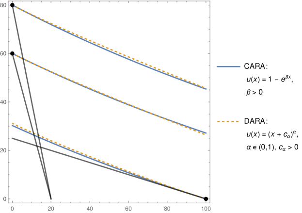
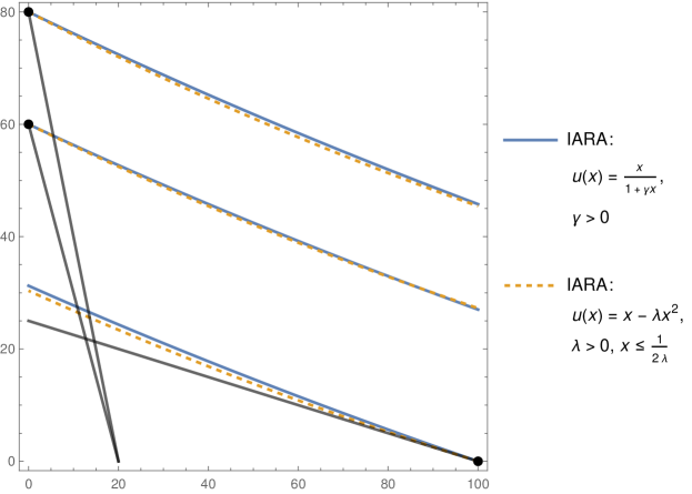
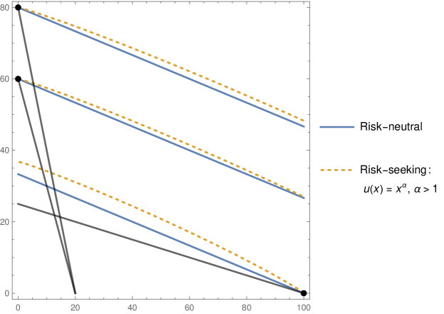
Figure 1: The example dataset with non-diversified demands affords SEU rationalizations under the same beliefs and 6 distinct risk preferences/attitudes.

Assume two states of the world and consider the non-diversified-demand example dataset

$$\mathcal{D}:=\left\{\underbrace{\big{(}(100,0),(1,4)\bigr{)}}_{(x^{1},\,p^{1})},\underbrace{\big{(}(0,80),(4,1)\bigr{)}}_{(x^{2},\,p^{2})},\underbrace{\big{(}(0,60),(3,1)\bigr{)}}_{(x^{3},\,p^{3})}\right\}.$$

It is easy to see that $\mathcal{D}$ satisfies the Generalized Axiom of Revealed Preference (GARP) and is therefore rationalizable by some ordinal utility index (Afriat, 1967). We also verify that it satisfies the Strong Axiom of Revealed Subjective Expected Utility (Echenique and Saito, 2015), which we recall next.

Strong Axiom of Revealed Subjective Expected Utility
For any sequence of pairs $(x_{\omega_{i}}^{k_{i}},x_{\omega^{\prime}_{i}}^{k^{\prime}_{i}})_{i=1}^{n}$ of demands in $\mathcal{D}$ in which the following statements are true, the product of prices corresponding to these demands satisfies $\prod_{i=1}^{n}\frac{p_{\omega_{i}}^{k_{i}}}{p_{\omega^{\prime}_{i}}^{k^{\prime}_{i}}}\leq 1$:
(i) $x_{\omega_{i}}^{k_{i}}>x_{\omega^{\prime}_{i}}^{k^{\prime}_{i}}$ for all $i$.
(ii) Each $\omega$ appears as $\omega_{i}$ in a pair the same number of times it appears as $\omega^{\prime}_{i}$.
(iii) Each $k$ appears as $k_{i}$ in a pair the same number of times it appears as $k^{\prime}_{i}$.

Indeed, for the two relevant sequences $(x^{1},x^{2})$ and $(x^{1},x^{3})$ in our example we observe that, for $j\in\{2,3\}$, $x^{1}_{1}>x^{j}_{1}$, $x^{j}_{2}>x^{1}_{2}$, $x^{1}_{1}>x^{1}_{2}$, $x^{j}_{2}>x^{j}_{1}$ and $\frac{p^{1}_{1}p^{j}_{2}}{p^{1}_{2}p^{j}_{1}}<1$. Hence, SARSEU is satisfied and, by Theorem 1 in Echenique and Saito (2015), there exists a concave and strictly increasing utility index $u$ and a full-support probability measure $\pi$ on $\Omega:=\{1,2\}$ that form a risk-averse SEU rationalization of $\mathcal{D}$.

We now illustrate our main results on this example dataset for the fixed beliefs $\pi:=\left(\frac{1}{4},\frac{3}{4}\right)$ (see also Fig. 1). With a utility index $u$, optimality of choice $x^{i}$ at prices $p^{i}$, $i\leq 3$, is equivalent to the marginal rate of substitution condition

$$\frac{\pi_{\omega^{i}}}{\pi_{\omega^{\prime}}}\frac{u^{\prime}(x^{i}_{\omega^{i}})}{u^{\prime}(0)} \geq \frac{p^{i}_{\omega^{i}}}{p^{i}_{\omega^{\prime}}}$$ (6)

In case (i.) with $u$ featuring $c_{\alpha}=1$ these conditions become $\frac{1}{3}\cdot 101^{\alpha-1}\geq\frac{1}{4}$, $3\cdot 81^{\alpha-1}\geq\frac{1}{4}$ and $3\cdot 61^{\alpha-1}\geq\frac{1}{3}$, and are simultaneously satisfied for $\alpha\in(0.9378,1)$, for example. In the CARA case (ii.), the conditions reduce to $\frac{1}{3}e^{-100\beta}\geq\frac{1}{4}$, $3e^{-80\beta}\geq\frac{1}{4}$ and $3e^{-60\beta}\geq\frac{1}{3}$. These inequalities are satisfied when $\beta<0.00285$, for example. For the quadratic-utility IARA index in (iii.), formulated as $u(x)=\theta x-\lambda x^{2}$, the conditions are $\frac{1}{3}\frac{\theta-200\lambda}{\theta}\geq\frac{1}{4}$, $3\frac{\theta-160\lambda}{\theta}\geq\frac{1}{4}$ and $3\frac{\theta-120\lambda}{\theta}\geq\frac{1}{3}$. These conditions are satisfied for any $\theta,\lambda$ such that $\theta\geq 800\lambda$. For the IARA index in (iv.) the conditions become $\frac{1}{3(1+100\gamma)^{2}}\geq\frac{1}{4}$, $\frac{3}{(1+80\gamma)^{2}}\geq\frac{1}{4}$, $\frac{3}{(1+60\gamma)^{2}}\geq\frac{1}{3}$ and are satisfied for all $\gamma\in\left(0,\frac{2\sqrt{3}-3}{300}\right]$. In the risk-neutral and risk-seeking cases (v.) and (vi.) with linear and strictly convex utility functions, finally, (6) is trivially satisfied because $\frac{u^{\prime}(x^{i}_{\omega^{i}})}{u^{\prime}(0)}\geq 1$ and $\frac{\pi_{\omega^{i}}}{\pi_{\omega^{\prime}}}\geq\frac{p^{i}_{\omega^{i}}}{p^{i}_{\omega^{\prime}}}$ for all $i$. $\lozenge$

References

- (1)
- Afriat (1967) Afriat, Sidney N., “The Construction of Utility Functions from Expenditure Data,” International Economic Review, 1967, 8, 67–77.
- Aliprantis and Border (2006) Aliprantis, Charalambos D. and Kim C. Border, Infinite Dimensional Analysis, 3rd edition, Berlin Heidelberg: Springer, 2006.
- Andreoni and Sprenger (2012) Andreoni, James and Charles Sprenger, “Estimating Time Preferences from Convex Budgets,” American Economic Review, 2012, 102, 3333–3356.
- Andreoni et al. (2015) , Michael A. Kuhn, and Charles Sprenger, “Measuring Time Preferences: A Comparison of Experimental Methods,” Journal of Economic Behavior & Organization, 2015, 116, 451–464.
- Augenblick et al. (2015) Augenblick, Ned, Muriel Niederle, and Charles Sprenger, “Working Over Time: Dynamic Inconsistency in Real Effort Tasks,” Quarterly Journal of Economics, 2015, pp. 1067–1115.
- Blow et al. (2022) Blow, Laura, Ian Crawford, and Vincent P. Crawford, “Meaningful Theorems: Nonparametric Analysis of Reference-Dependent Preferences,” Working Paper, 2022.
- Chambers et al. (2016a) Chambers, Christopher P, Ce Liu, and Seung-Keun Martinez, “A Test for Risk-Averse Expected Utility,” Journal of Economic Theory, 2016, 163, 775–785.
- Chambers et al. (2016b) Chambers, Christopher P., Federico Echenique, and Kota Saito, “Testing Theories of Financial Decision Making,” Proceedings of the National Academy of Sciences, 2016, 113, 4003–4008.
- Chambers et al. (2021) , , and Nicolas Lambert, “Recovering Preferences from Finite Data,” Econometrica, 2021, 89, 1633–1664.
- Chen et al. (2022) Chen, Jie, Xunhua Su, Xuan Tian, and Bin Xu, “Does Customer-Base Structure Influence Managerial Risk-Taking Incentives?,” Journal of Financial Economics, 2022, 143, 462–483.
- Choi et al. (2007) Choi, Syngjoo, Raymond Fisman, Douglas Gale, and Shachar Kariv, “Consistency and Heterogeneity of Individual Behavior under Uncertainty,” American Economic Review, 2007, 97, 1921–1938.
- Echenique and Saito (2015) Echenique, Federico and Kota Saito, “Savage in the Market,” Econometrica, 2015, 83, 1467–1495.
- Epstein (2000) Epstein, Larry G., “Are Probabilities Used in Markets?,” Journal of Economic Theory, 2000, 91, 86–90.
- Green et al. (1979) Green, J. R., L. J. Lau, and H. M. Polemarchakis, “On the Recoverability of the von Neumann-Morgenstern Utility Function From Asset Demands,” in J. R. Green and J. A. Scheinkman, eds., Equilihrium, Growth and Trade: Essays in Honor of L. McKenzie, New York: Academic Press, 1979, pp. 151–161.
- Green and Srivastava (1986) Green, Richard C. and S. Srivastava, “Expected Utility Maximization and Demand Behavior,” Journal of Economic Theory, 1986, 38, 313–323.
- Halevy et al. (2018) Halevy, Yoram, Dotan Persitz, and Lanny Zrill, “Parametric Recoverability of Preferences,” Journal of Political Economy, 2018, 126 (4), 1558–1593.
- Heufer (2014) Heufer, Jan, “Nonparametric Comparative Revealed Risk Aversion,” Journal of Economic Theory, 2014, 153, 569–616.
- Inada (1963) Inada, Ken-Ichi, “On a Two-Sector Model of Economic Growth: Comments and a Generalization,” Review of Economic Studies, 1963, 30, 119–127.
- Kübler and Polemarchakis (2017) Kübler, Felix and Herakles Polemarchakis, “Identification of Beliefs from Asset Demand,” Econometrica, 2017, 85, 1219–1238.
- Kübler et al. (2014) , Larry Selden, and Xiao Wei, “Asset Demand Based Tests of Expected Utility Maximization,” American Economic Review, 2014, 104, 3459–3480.
- Kübler et al. (2021) , Raghav Malhotra, and Herakles Polemarchakis, “Exact Inference from Finite Market Data,” Working Paper, 2021.
- Ogaki and Zhang (2001) Ogaki, Masao and Qiang Zhang, “Decreasing Relative Risk Aversion and Tests of Risk Sharing,” Econometrica, 2001, 69, 515–526.
- Polisson et al. (2020) Polisson, Matthew, John K.-H. Quah, and Ludovic Renou, “Revealed Preferences over Risk and Uncertainty,” American Economic Review, 2020, 110, 1782–1820.
- Rockafellar (1970) Rockafellar, R. Tyrrell, Convex Analysis, Princeton: Princeton University Press, 1970.
- Savage (1954) Savage, Leonard J., The Foundations of Statistics, New York: Wiley, 1954.