Novel Quality Measure and Efficient Resolution of Convex Hull Pricing for Unit Commitment

Abstract

Electricity prices determined by economic dispatch that do not consider fixed costs may lead to significant uplift payments. However, when fixed costs are included, prices become non-monotonic with respect to demand, which can adversely impact market transparency. To overcome this issue, convex hull (CH) pricing has been introduced for unit commitment with fixed costs. Several CH pricing methods have been presented, and a feasible cost has been used as a quality measure for the CH price. However, obtaining a feasible cost requires a computationally intensive optimization procedure, and the associated duality gap may not provide an accurate quality measure. This paper presents a new approach for quantifying the quality of the CH price by establishing an upper bound on the optimal dual value. The proposed approach uses Surrogate Lagrangian Relaxation (SLR) to efficiently obtain near-optimal CH prices, while the upper bound decreases rapidly due to the convergence of SLR. Testing results on the IEEE 118-bus system demonstrate that the novel quality measure is more accurate than the measure provided by a feasible cost, indicating the high quality of the upper bound and the efficiency of SLR.

[inst1]organization=Department of Electrical and Computer Engineering, University of Connecticut,city=Storrs, postcode=06269, state=CT, country=USA

[inst2]organization=Electrical and Microelectronic Engineering, Rochester Institute of Technology,city=Rochester, postcode=14623, state=NY, country=USA

[inst4]organization=Advanced Technology and Solutions, ISO New England,city=Holyoke, postcode=01040, state=MA, country=USA

1 Introduction

In the electricity markets of the United States, prices are usually determined based on the economic dispatch (ED) problem [1]. However, since commitment costs such as start-up and no-load costs are not factored in, uplift payments may become substantial. When prices are determined based on the unit commitment (UC), which does account for such costs, the associated binary commitment-related variables lead to non-convexity. Consequently, prices based on a UC problem are non-monotonic with respect to demand [2], thereby reducing market transparency.

Convex hull (CH) pricing has been introduced as a possible resolution to the issues associated with fixed costs, binary variables, uplift payments, and non-monotonic prices based on the unit commitment (UC) problem [2]. CH pricing continues to be an active area of research today [3, 4]. One approach to obtaining CH prices is to solve the dual problem of the UC problem, with optimal CH prices representing optimal Lagrangian multipliers ($\lambda^{*}$) [5, 6]. The difference between a feasible cost to the UC problem and a dual value yields the uplift payment. However, this approach can face challenges related to the convergence of Lagrangian multipliers by using standard subgradient methods associated with high computational effort as well as multiplier zigzagging [7]. Various methods have been proposed to solve the CH pricing problem, with the quality of the resulting CH prices typically measured using a feasible cost that quantifies their proximity to the optimal prices, i.e., duality gap [8].

Challenges related to the current quality-measuring approach include 1. the substantial computational effort needed to obtain a feasible cost, and 2. a potentially insufficiently tight duality gap to provide a high-quality measure, as illustrated schematically in Figure 1 below. Consequently, a more robust alternative measure (upper bound) is desired. The innovative CH price quality measure is defined as the difference between the upper and lower bounds of the optimal dual value. While the lower bound can be derived from the best available dual value, a novel approach to determining the upper bound is necessary.

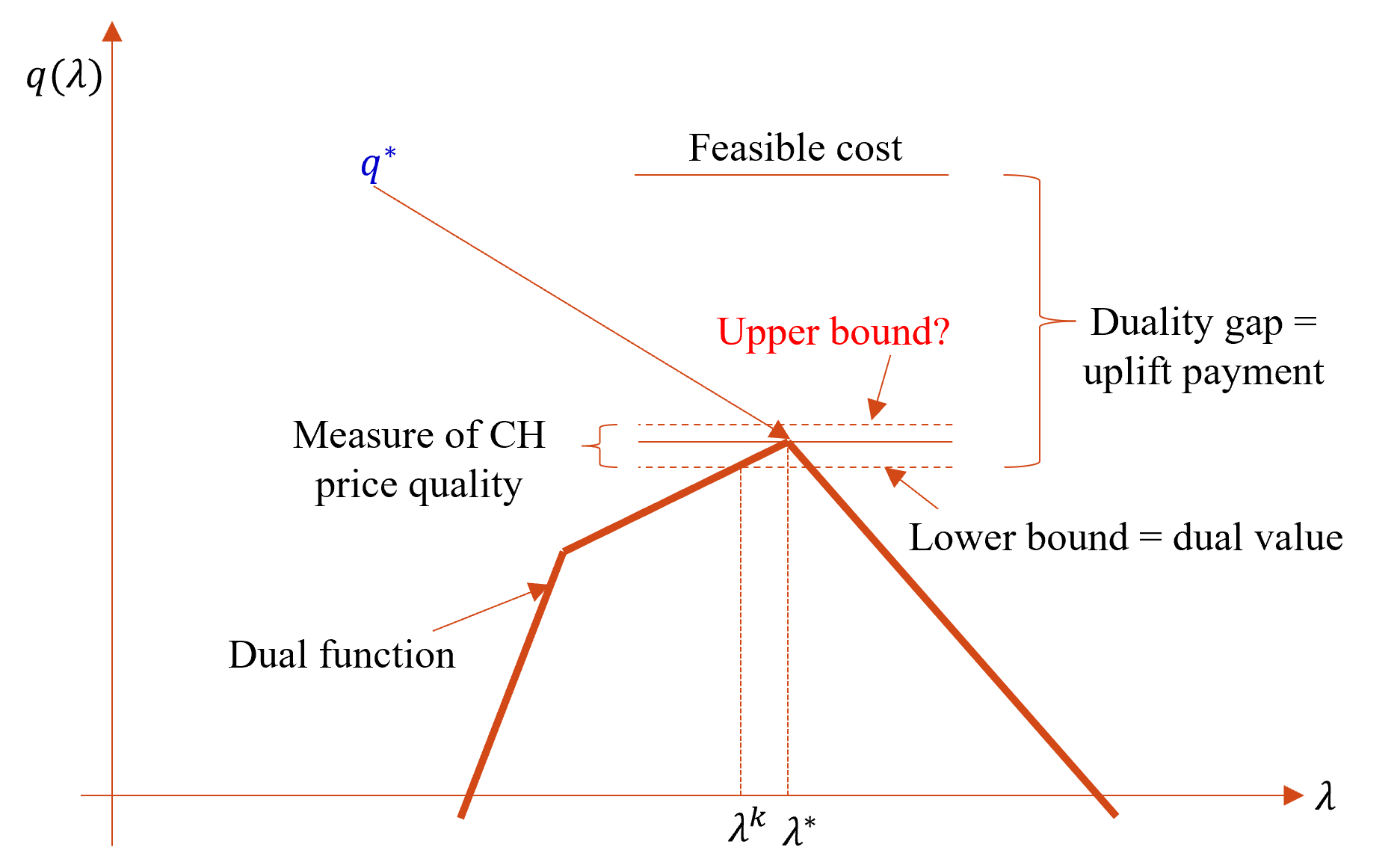
Figure 1: A schematic demonstration of a dual function, feasible cost, standard duality gap, and the novel proposed measure of CH price-quality.

This paper aims to provide a high-quality measure of CH prices through the development of a novel upper bound to the optimal dual value and the efficient computation of CH prices. We first present the UC problem in Section 2 and then develop a CH-price quality measure based on the difference between the innovative upper bound $\bar{q}$ and the best available dual value ($q(\lambda^{k})$) in Section 3. The near-optimal CH prices are obtained using the Surrogate Lagrangian Relaxation (SLR) method [9], which overcomes the challenges of standard sub-gradient methods and offers fast convergence of multipliers as well as the upper bound to the optimal dual value. Testing results based on the IEEE 118-bus system demonstrate the superiority of the proposed CH-price quality measure and the efficiency of the SLR method.

2 UC Problem Formulation for Convex Hull Pricing

This section presents the formulation of the UC problem, which serves as the foundation for the development of a novel CH-price quality measure and further presentation of CH prices. The section is divided into two subsections: subsection 2.1 focuses on the formulation without transmission constraints, which are frequently omitted in existing literature for the calculation of CH prices, and subsection 2.2 includes transmission constraints for a more realistic representation of the power system.

2.1 Unit Commitment Formulation without Transmission Constraints

Consider a UC problem with $I$ units indexed by $i$ and $T$ hours indexed by $t$.

1. Objective Function: The goal is to minimize the total cost as:

   $$\min_{\left\{x_{i},u_{i},p_{i},r_{i}\right\}}{\left\{\sum_{i=1}^{I}{z_{i}\left(x_{i},u_{i},p_{i},r_{i}\right)}\right\}},$$ (1)

   where $z_{i}\left(x_{i},u_{i},p_{i},r_{i}\right)=\displaystyle\sum_{t=1}^{T}\left(c_{i}^{E}\left(p_{i,t}\right)+c_{i}^{S}\cdot u_{i,t}+c_{i}^{N}\cdot x_{i,t}\right)$ represents the total cost of unit $i$, including energy costs, start-up costs, and no-load costs. Decision variables at time $t$ are: 1. binary commitment $x_{i,t}$ and start-up $u_{i,t}$; and 2. continuous dispatch $p_{i,t}$ .

2. System-Wide Constraints

   System Demand: The total power generation equals the demand at each time $t$:

   $$\sum_{i=1}^{I}p_{i,t}=D_{t},t=1,\ldots,T,$$ (2)

   where $p_{i,t}$ are generation levels and $D_{t}$ is the demand at time $t$.

3. Unit-Level Constraints

   1. Generation Capacity Constraints: The generation capacity for online units $(x_{i,t}=1)$ is restricted by a lower limit and an upper limit, denoted by $P_{i}^{min}$ and $P_{i}^{max}$, respectively. Meanwhile, when a unit is offline, represented by the corresponding commitment status $x_{i,t}=0$, its generation level is zero. The mathematical constraints capturing these relationships are provided below:

      $$x_{i,t}\cdot P_{i}^{min}\leq p_{i,t}\leq x_{i,t}\cdot P_{i}^{max},$$ (3)

   2. Start-Up Constraints: Start-ups are captured by using binary variables $u_{i,t}$ as:

      $$x_{i,t}-x_{i,t-1}\leq u_{i,t}.$$ (4)

      In the above relationship, a start-up cost is incurred when $u_{i,t}=1,$ which is only possible when $x_{i,t}=1$ and $x_{i,t-1}=0.$

   3. Minimum Up- and Down-Time Constraints: Unit $i$ stays online (offline) for its minimum up- (down-) time $l_{i}(L_{i})$:

      $$\sum_{j=t-L_{i}+1}^{t}u_{i,j}\leq x_{i,t},\ \sum_{j=t-l_{i}+1}^{t}u_{i,j}\leq 1-x_{i,t-l_{i}}.$$ (5)

   4. Ramp-Rate Constraints: The change of generation levels between two consecutive hours cannot exceed its ramp-rate requirements:

      $$p_{i,t}-p_{i,t-1}\leq R_{i}\cdot x_{i,t-1}+V_{i}\cdot\left(1-x_{i,t-1}\right),$$ (6)

      $$p_{i,t-1}-p_{i,t}\leq R_{i}\cdot x_{i,t}+V_{i}\cdot\left(1-x_{i,t}\right),$$ (7)

      where $R_{i}$ are ramp-up/down and $V_{i}$ is the start-up/shut-down ramp rates.

2.2 Unit Commitment Formulation with Transmission Constraints

The above UC problem formulation does not consider transmission constraints. However, transmission constraints are often included in practical situations. In such cases, the following constraints are added to the formulation instead of the demand constraint in (2):

1. DC Power Flow Constraints: The power flow on each transmission line $l$ at time $t$ is given by:

   $$f_{l,t}=\frac{\theta_{s\left(l\right),t}-\theta_{r\left(l\right),t}}{X_{l}},l=1,\ldots,L,t=1,\ldots,T.$$ (8)

   Here $\theta_{s\left(l\right),t}$ and $\theta_{r\left(l\right),t}$ are phase angles at sending and received buses of line $l$, and $X_{l}$ is line $l$ impedance.

2. Nodal Flow Balance Constraints: Nodal flow balance is maintained at each node $n$=1,$\ldots,N$ by the following equation:

   $$\sum_{l:r\left(l\right)=n}f_{l,t}+p_{n,t}=\sum_{l:s\left(l\right)=n}f_{l,t}+D_{n,t},\ t=1,\ldots,T.$$ (9)

3. Transmission Capacity Constraints: The power flow on each transmission line $l$ is limited by its minimum and maximum capacity:

   $$f_{l}^{min}\leq f_{l,t}\leq f_{l}^{max},l=1,\ldots,L,t=1,\ldots,T.$$ (10)

3 Convex Hull Pricing through the Dual Problem

This section is on the development of a novel measure to quantify CH-price quality. After briefly presenting a dual problem in subsection 3.1 as well as the SLR method in subsection 3.2, the novel measure is developed in subsection 3.3.

3.1 The Dual Problem of the UC Problem

For simplicity, the explanation will rest upon the formulation with system demand constraints; a formulation with transmission constraint follows analogously. The dual problem to the UC problem is defined as [10]:

$$\max_{\lambda}q(\lambda),$$ (11)

where $q(\lambda)$ is the dual function defined as:

$$q\left(\lambda\right)=\min_{\left\{p,x,u\right\}\in\mathfrak{F}}{L\left(\lambda,p,x,u\right)}.$$ (12)

Here $\mathfrak{F}$ is a feasible set delineated by constraints (3)-(7), the minimization within (12) is the “relaxed problem,” and $L\left(\lambda,p,x,u\right)$ is the Lagrangian function defined as:

$$L\left(\lambda,p,x,u\right)=\sum_{i=1}^{I}{z_{i}\left(x_{i},u_{i},p_{i}\right)}+\lambda\cdot g(p),$$ (13)

where $\lambda=\left\{\lambda_{t}\right\}$ is a vector of Lagrangian multipliers obtained after relaxing demand constraints (2). The corresponding constraint violations are collectively denoted as $g(p)$ for the compactness of notation. The CH prices are optimal multipliers $\lambda^{\ast}$ of the dual problem (11) [2].

The methodology to be presented will be based on the above. Extension for the formulation with transmission follows the same logic with the exception that nodal flow balance constants (9) are relaxed rather than system demand constraints (2), in which case the multipliers $\lambda$ will be a matrix.

3.2 Surrogate Lagrangian Relaxation Method [9]

In this subsection, our recent Surrogate Lagrangian Relaxation (SLR) Method will be briefly introduced. Within the method, multipliers are updated based on “surrogate” subgradients $g\left(\tilde{p}^{k}\right)$ (which are levels of constraint violations of relaxed constraints), and stepsizes $s_{SLR}^{k}$ as:

$$\lambda_{t}^{k+1}=\lambda_{t}^{k}+s_{SLR}^{k}\cdot g\left(\tilde{p}^{k}\right),$$ (14)

where,

$$s_{SLR}^{k}=\left(1-\frac{1}{M\cdot k^{1-\frac{1}{k^{\rho}}}}\right)\cdot s_{SLR}^{k-1}\cdot\frac{||g(\tilde{p}^{k-1})||}{||g(\tilde{p}^{k})||},M>1,0<\rho<1.$$ (15)

Here, “tilde” ($\texttildelow$) indicates that optimization of the relaxed problem is subject to the following “surrogate optimality condition” [9, p. 178, eq. (12)]: $L\left(\lambda^{k},\ \tilde{x}^{k},\ \tilde{u}^{k},\ \tilde{p}^{k}\right)<$ $L\left(\lambda^{k},\ \tilde{x}^{k-1},\ \tilde{u}^{k-1},\ \tilde{p}^{k-1}\right)$, rather than to full minimization the Lagrangian function in (12), with $L\left(\lambda^{k},\ \tilde{x}^{k},\ \tilde{u}^{k},\ \tilde{p}^{k}\right)$ being a “surrogate dual value” (a value that the Lagrangian function (13) attains at solutions $\tilde{x}^{k},\ \tilde{u}^{k},\ \tilde{p}^{k}$). The primary advantages of the SLR method lie in the fact that it does not require solving all sub-problems simultaneously and only needs to satisfy the surrogate optimality condition mentioned earlier. Both of these factors contribute to a significant reduction in computational effort. Moreover, surrogate directions do not change drastically from one iteration to the next, and zigzagging difficulties are thus alleviated. Thereby also contributing to the overall significant reduction of the computational effort.

3.3 Novel Quality Measure for Convex Hull Pricing

This subsection is on a novel way to obtain the upper bound $\bar{q}$ to the optimal dual value $q\left(\lambda^{\ast}\right)$, approaching $q\left(\lambda^{\ast}\right)$ from above. Together with dual values $q\left(\lambda^{k}\right)$ (which are a lower bound), the novel CH-price quality measure will be obtained as a relative difference between $\bar{q}$ and $q\left(\lambda^{k}\right)$.

As proved within the “Surrogate” Subgradient Method (SSM) [11, pp. 704-706], if the following condition on stepsizes holds

$$s^{k}<\frac{q^{*}-\tilde{L}(\lambda^{k},x^{k},u^{k},p^{k})}{||\tilde{g}(p^{k})||^{2}},$$ (16)

then multipliers approach $\lambda^{*}$ at every iteration:

$$||\lambda^{*}-\lambda^{k+1}||^{2}<||\lambda^{*}-\lambda^{k}||^{2}.$$ (17)

However, the optimal dual value $q^{*}$ required to set stepsizes is generally not known for any given problem. Therefore, when stepsizes are set by using any other rule without using $q^{*}$, then multipliers may not approach $\lambda^{*}$ (or any other point) at every iteration. This “non-approaching” property will be exploited to derive the novel quality measure. Specifically, if one can detect that multipliers do not approach $\lambda^{*}$, then this is only because stepsizes are “too large,” that is, stepsizes violate (16). This result is summarized in the following Lemma.

Lemma: If there exists $\kappa$ so that $\lambda^{\ast}$ move away from $\lambda^{\ast}$, i.e.,

$$||\lambda^{*}-\lambda^{k+1}||^{2}\geq||\lambda^{*}-\lambda^{k}||^{2},$$ (18)

then

$$s^{\kappa}\geq\frac{q^{*}-\tilde{L}(\lambda^{\kappa},x^{\kappa},u^{\kappa},p^{\kappa})}{||\tilde{g}(p^{\kappa})||^{2}}.$$ (19)

Proof: Denote (16) as assertion A and (17) as B. According to [11, pp. 704-706], the following predicate holds true: $\forall k:\ A\rightarrow B$. In the proof, the following relation will be helpful:

$$\lnot\left(A\rightarrow B\right)=\lnot A\vee B.$$ (20)

Negation of the predicate $\forall k:\ A\rightarrow B$ leads to $\exists k:\ \lnot(A\rightarrow B)$, which simplifies to $\exists k:\ \lnot A\vee B$, which is equivalent to $\exists k:\ B\vee\left(\lnot A\right)$ by the commutative property of disjunctions. By (20), the latter predicate is equivalent to $\exists k:(\lnot B)\rightarrow\left(\lnot A\right)$.

According to (18), there exists an overestimate of the optimal dual value $\bar{q}>q^{\ast}$ such that

$$s^{\kappa}\geq\frac{\bar{q}-\tilde{L}(\lambda^{\kappa},x^{\kappa},u^{\kappa},p^{\kappa})}{||\tilde{g}(p^{\kappa})||^{2}}.$$ (21)

From (21), the overestimate can be expressed as:

$$\bar{q}=s^{\kappa}||\tilde{g}(p^{\kappa})||^{2}+\tilde{L}(\lambda^{\kappa},x^{\kappa},u^{\kappa},p^{\kappa}).$$ (22)

However, the difficulty is that (22) was determined based on the inequality (18) which involves the unknown $\lambda^{\ast}$, and the upper bound (22) cannot be computed. To resolve this difficulty, the following assumption is used.

Assumption: Assuming that multipliers (14) generated by the SLR method do not approach any common value (including $\lambda^{\ast}$) during several iterations, which is a realistic assumption because stepsizes (14) are not set by using (16) with an unknown $q^{*}$, then conditions (19), (21) and (22) hold. To determine whether multipliers approach any common value or not, the following “multiplier divergence detection” problem (23) is solved where divergence is detected if (23) is infeasible (the multipliers diverge instead of converging):

$$\begin{gathered}||\lambda-\lambda^{k+1}||^{2}\leq||\lambda-\lambda^{k}||^{2},\\ ||\lambda-\lambda^{k+2}||^{2}\leq||\lambda-\lambda^{k+1}||^{2},\\ \cdots\\ ||\lambda-\lambda^{k+n}||^{2}\leq||\lambda-\lambda^{k+n-1}||^{2}.\end{gathered}$$ (23)

With respect to (23), $\lambda$ is a vector of continuous decision variables (not to be confused with dual variables within (11)).

The above assumption is realistic. Otherwise, multipliers would always strictly approach $\lambda^{\ast}$ and converge to $\lambda^{\ast}$. The latter is by the design of the SLR method [9], yet, the former can only be guaranteed if the SSM stepsize (16) is used.

The problem (23) is set up starting from values $\lambda^{k}$ and $\lambda^{k+1}$ and one inequality. After $\lambda^{k+2}$ is obtained, the second inequality is added, and so on until a certain $k+n-1$ ($n$ is not known beforehand) iteration is reached whereby (23) is infeasible.

Since at one of the iterations $k,\dots,k+n-1$, equality (19) holds, the sought-for upper bound is then obtained as:

$$\bar{q}=\max_{\kappa\in[k+1,k+n]}\{s^{\kappa}\cdot\textbardbl\tilde{g}(p^{\kappa})\textbardbl^{2}+\tilde{L}(\lambda^{\kappa},x^{\kappa},u^{\kappa},p^{\kappa})\}.$$ (24)

Subsequently, values of $k$ and $n$ are reset as $k\rightarrow k+n,\ n\rightarrow 1$, and the procedure repeats.

Finally, the quality measure of the CH prices is defined as $\frac{{\bar{q}}^{k}-q^{k}}{{\bar{q}}^{k}}$, where ${\bar{q}}^{k}$ is the best (lowest) upper bound, and $q^{k}$ is the best (highest) dual value obtained up to iteration $k$. This measure can be used as a stopping criterion.

Unlike feasible costs, the novel upper bound approaches the optimal dual value from above since the upper bound (24) depends on the stepsizes approaching zero and the Lagrangian function approaching the optimal dual value, as proved in [9]. Another implication of the above is that the fast convergence of SLR leads to fast convergence of the upper bound to the optimal dual value.

4 Numerical Testing

This section is to demonstrate the performance of the novel quality measure of CH prices by comparing it with the duality gap of the problem. In Example 1, a small 2-unit UC problem is considered. In Examples 2 and 3, a UC problem based on the IEEE 118-bus system without and with transmission capacity constraints is considered. Within all examples, 24 hours are considered. The method is implemented using IBM ILOG CPLEX Optimization Studio V 12.10.0.0 on a PC with a 2.40 GHz Intel® Xeon® E-2286M CPU and 32G RAM.

4.1 Example 1. Small Example without transmission capacity constraints

Consider a UC problem with two units with the following characteristics:

• Unit 1: Pmin = 50 MW, Pmax = 200 MW, initial ramp rate = 150.3 MW/hr and general ramp rate = 200.6 MW/hr, generation cost: 65 $/MW and start-up cost: 0.

• Unit 2: Pmin = 50 MW, Pmax = 200 MW, initial ramp rate = 70.35 MW/hr and general ramp rate = 40.7 MW/hr, generation cost: 40 $/MW, start-up cost: $6000.

The results are shown in Figure 2. Our SLR method obtains near-optimal CH prices with a quality of 0.012% in 40 sec. Compared to the duality gap of 10.51%, the novel quality measure of 0.012% is significantly more accurate. The amount of time required to obtain the upper bound is 0.448 sec, which is roughly 1% of the total time (40 sec). The amount of time required to obtain the feasible cost is slightly longer at 0.6 sec.

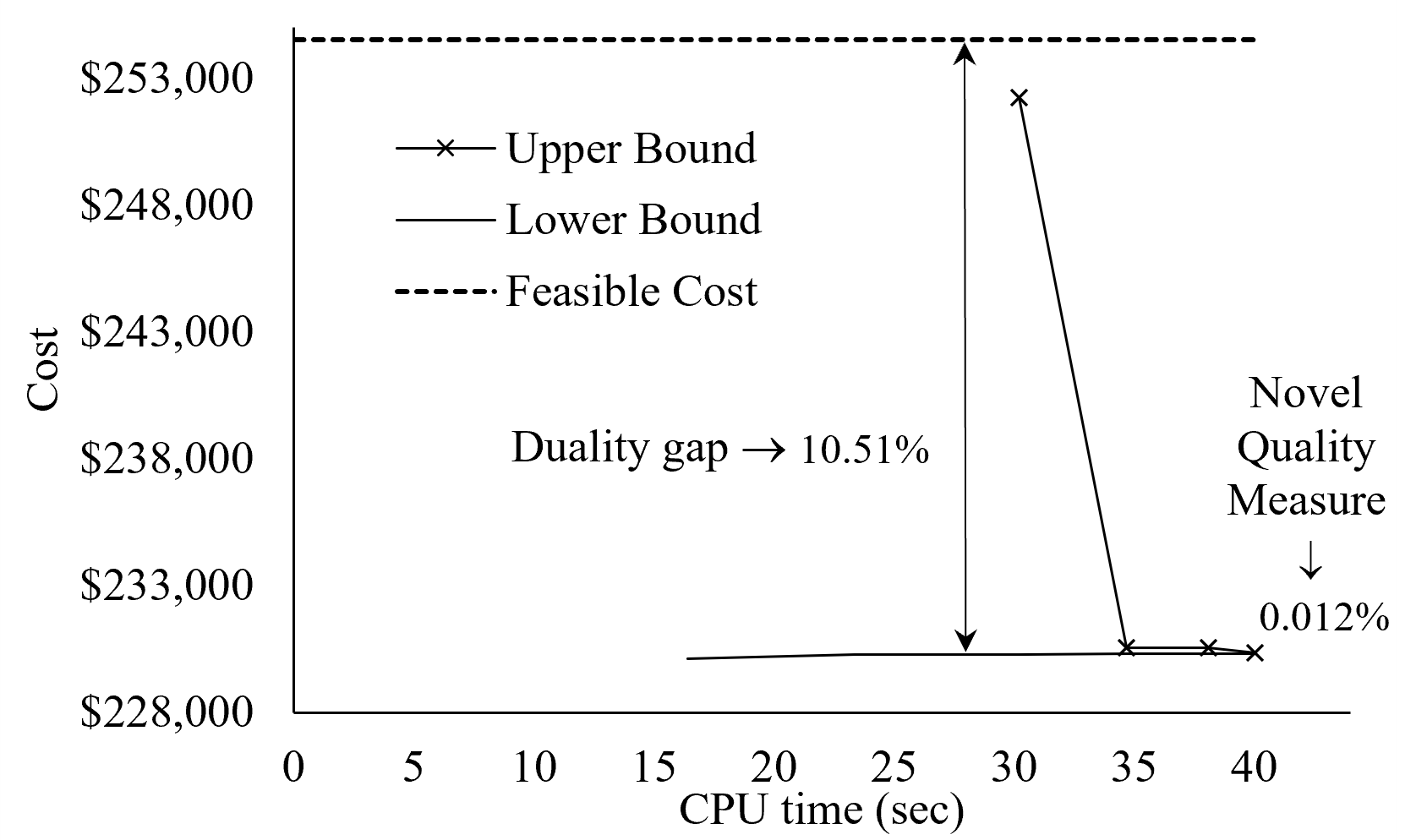
Figure 2: Results for Example 1

4.2 Example 2. IEEE 118-bus Case without transmission capacity constraints

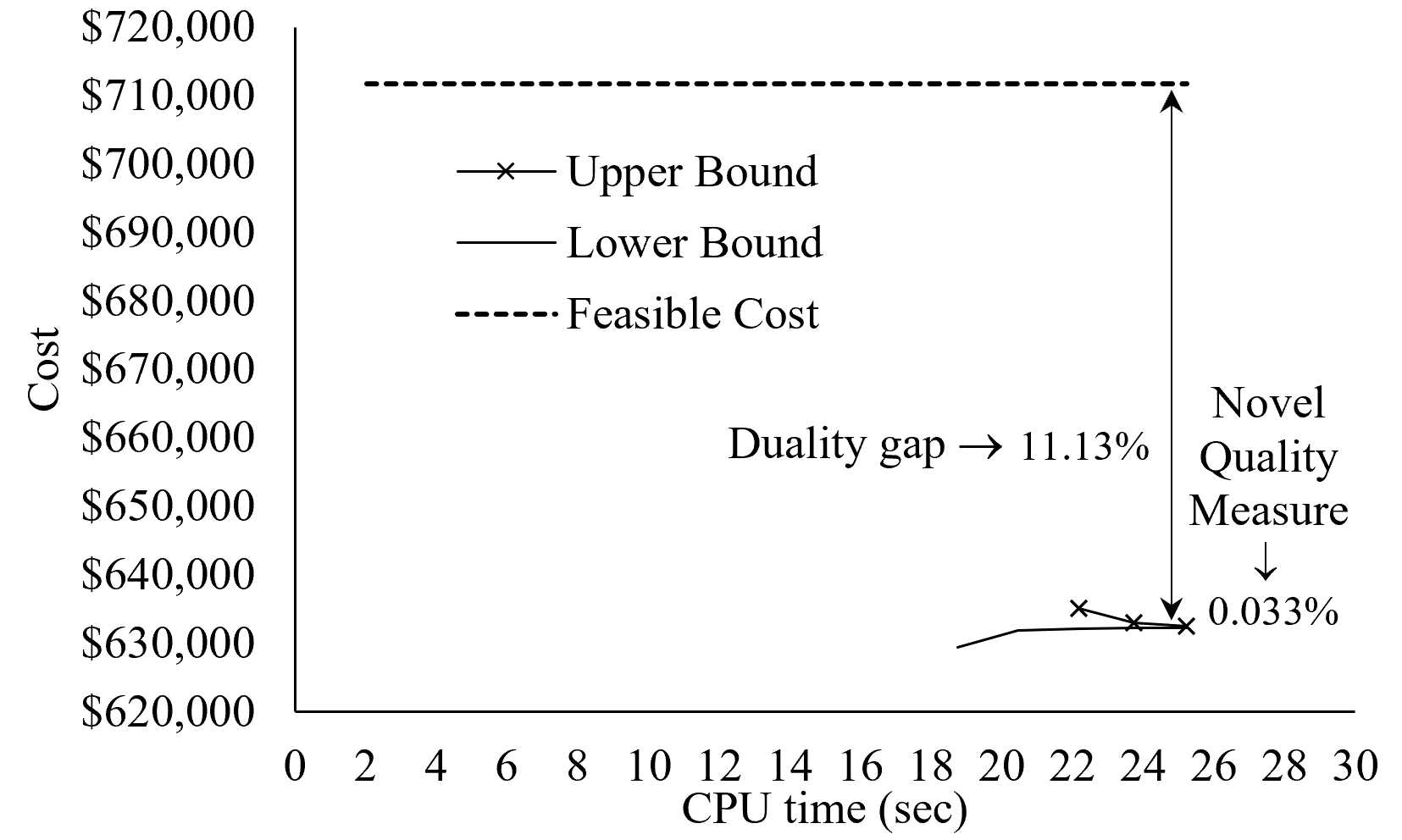
Figure 3: Results for Example 2

Consider a 54-unit, 24-hour UC problem based on the IEEE 118-bus system. The results are shown in Figure 3. Compared to the duality gap of 11.13%, the novel quality measure of 0.033% is significantly more accurate. Near-optimal CH prices with a quality of 0.033% are obtained in 25 sec. The amount of time required to obtain the upper bound is 0.617 sec, which is roughly 2.2% of the total time. The amount of time required to obtain the feasible cost is slightly longer at 0.647 sec.

4.3 Example 3. IEEE 118-bus Case with transmission capacity constraints

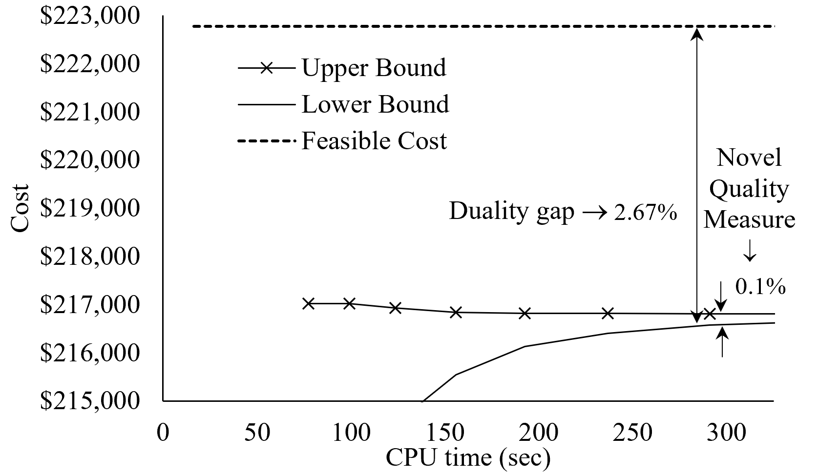
Figure 4: Results for Example 3

Consider the same problem of Example 2 with transmission capacity constraints. The results obtained by using SLR are shown in Figure 4. Near-optimal CH prices with quality of 0.1% are obtained in 290 sec. Compared to the duality gap of 2.67%, the novel quality measure of 0.1% is more accurate. The amount of time required to obtain the upper bound is 0.7 sec, which is roughly 0.22% of the total time. The amount of time required to obtain the feasible cost is longer at 1.57 sec.

Based on the three examples described above, the following observations can be made:

1. The results of Example 4.2 (118-bus without transmission capacity constraints) are comparable to those obtained for a smaller problem of Example 4.1, in terms of CPU time and CH-price quality. The novel quality measure is significantly more accurate than the duality gap.

2. The results of Example 4.3 (118-bus with transmission capacity constraints) show the impact of transmission line constraints on solving time and CH-price. However, the novel quality measure is still more accurate than the duality gap.

3. Compared to the problem-dependent standard duality gaps, which may be large, the novel quality measures are problem-independent and are more accurate.

Computationally, the standard quality gap requires a feasible solution. When the number of units increases, the time required to obtain a feasible solution is expected to increase. The CPU time required to compute the novel quality measure is not expected to increase for larger-scale problems since the number of decision variables within (23) is independent of the number of units, paving the way for providing a tight measure of CH prices for large-scale problems within a modest CPU time.

5 Conclusions

In this paper, a novel measure for CH prices is developed and the near-optimal CH prices are efficiently obtained by using our recent SLR method. Through numerical testing, it is demonstrated that the near-optimal CH prices with high quality are obtained fast and the computational effort involved in obtaining an upper bound for the CH-price quality measure takes a fraction of the total solving time. The method to quantify the quality of CH prices is generic within the LR-based methods and can be generally used to quantify the quality of the dual solutions.

References

- [1] E. Litvinov, F. Zhao, T. Zheng, Electricity markets in the united states: Power industry restructuring processes for the present and future, IEEE Power and Energy Magazine 17 (1) (2019) 32–42.
- [2] P. R. Gribik, W. W. Hogan, S. L. Pope, et al., Market-clearing electricity prices and energy uplift, Cambridge, MA (2007) 1–46.
- [3] P. Andrianesis, D. Bertsimas, M. C. Caramanis, W. W. Hogan, Computation of convex hull prices in electricity markets with non-convexities using dantzig-wolfe decomposition, IEEE Transactions on Power Systems 37 (4) (2021) 2578–2589.
- [4] N. Stevens, A. Papavasiliou, Application of the level method for computing locational convex hull prices, IEEE Transactions on Power Systems 37 (5) (2022) 3958–3968.
- [5] C. Wang, T. Peng, P. B. Luh, P. Gribik, L. Zhang, The subgradient simplex cutting plane method for extended locational marginal prices, IEEE Transactions on Power Systems 28 (3) (2013) 2758–2767.
- [6] G. Wang, U. V. Shanbhag, T. Zheng, E. Litvinov, S. Meyn, An extreme-point subdifferential method for convex hull pricing in energy and reserve markets—part i: Algorithm structure, IEEE Transactions on Power Systems 28 (3) (2013) 2111–2120.
- [7] P. B. Luh, D. Zhang, R. N. Tomastik, An algorithm for solving the dual problem of hydrothermal scheduling, IEEE Transactions on Power Systems 13 (2) (1998) 593–600.
- [8] Y. Yu, T. Zhang, Y. Guan, Y. Chen, Convex primal formulations for convex hull pricing with reserve commitments, IEEE Transactions on Power Systems 36 (3) (2020) 2345–2354.
- [9] M. A. Bragin, P. B. Luh, J. H. Yan, N. Yu, G. A. Stern, Convergence of the surrogate lagrangian relaxation method, Journal of Optimization Theory and applications 164 (2015) 173–201.
- [10] B. Hua, R. Baldick, A convex primal formulation for convex hull pricing, IEEE Transactions on Power Systems 32 (5) (2016) 3814–3823.
- [11] X. Zhao, P. B. Luh, J. Wang, Surrogate gradient algorithm for lagrangian relaxation, IEEE Transactions on Power Systems 32 (5) (1999) 3814–3823.