Snacks: a fast large-scale kernel SVM solver

Abstract

Kernel methods provide a powerful framework for non parametric learning. They are based on kernel functions and allow learning in a rich functional space while applying linear statistical learning tools, such as Ridge Regression or Support Vector Machines. However, standard kernel methods suffer from a quadratic time and memory complexity in the number of data points and thus have limited applications in large-scale learning. In this paper, we propose Snacks, a new large-scale solver for Kernel Support Vector Machines. Specifically, Snacks relies on a Nyström approximation of the kernel matrix and an accelerated variant of the stochastic subgradient method. We demonstrate formally through a detailed empirical evaluation, that it competes with other SVM solvers on a variety of benchmark datasets.

I Introduction

Linear statistical learning models are well-studied, convenient to use, to analyze, and they often lead to computationally efficient algorithms [1]. However, they assume a linear relation between inputs and outputs and thus often fail to fit complex datasets properly. Kernel methods propose a tractable non-linear extension to linear statistical learning models [2, 3], based on positive-definite kernels. Intuitively, a positive-definite kernel corresponds to a similarity measure between elements of the input space. Such kernels serve as a non-linear mapping which sends the data to a high-dimensional feature space. Computing linear models in this feature space corresponds to computing a non-linear model in the original space. The non-linear function that is learned depends on the kernel function used. As good choices of the kernel function can lead to linearly separable data in the feature space, this approach has been proven successful in many areas such as bioinformatics, signal processing and visual recognition [4]. Kernel methods are based on a rigorous mathematical framework that stems from functional analysis and the theory of reproducing kernel Hilbert spaces [5, 2, 7] and statistical results can be derived as an extension of linear statistical learning models [9, 11].

Support Vector Machines (SVMs) are historically the first kernel method used for pattern recognition [13, 2]. They have been widely used in many contexts such as image classification, text classification [14] or protein fold recognition [16]. Among kernel methods, SVMs are quite popular and represent the state-of-the-art in many contexts. Unlike many learning algorithms (especially neural networks), SVMs solve a convex optimization problem. This presents a substantial advantage as the structure of the SVM classifier is entirely data-driven once a suitable kernel is chosen. However, kernel methods require storing a kernel matrix that grows quadratically with the number of samples, limiting SVM solvers to small-scale or medium-scale problems. This bottleneck has been previously addressed through various approaches. Exact solvers consider fast optimization algorithms and often decompose the problem by chunking methods [17, 18, 19, 20]. Approximate solvers, on the other hand, rely on random features [9, 21, 22] or Nyström subsampling [23, 24] to reduce the computational cost by considering random projections of the original space, often without leading to any degradation in terms of learning performance [8, 25].

I-A Overview of Snacks

This paper describes Snacks, a primal kernel SVM algorithm for classification which can handle large-scale datasets. Our proposed kernel algorithm relies on

1. a Nyström approximation to tackle the quadratic complexity inherent to kernel methods and reduce the computational burden [25],

2. an accelerated stochastic subgradient algorithm (ASSG) presented in [30] to solve the underlying convex optimization problem

Worst-case convergence results (Theorem 1 and 2) are complemented with numerical experiments on large datasets showing that our algorithm competes with state-of-the-art kernel SVM solvers in terms of training time and classification error.

I-B Related work

Beyond the references cited above, many kernel SVM solvers have been proposed in recent years. They can be divided into two categories based on which formulation they tackle. Some solvers, such as Pegasos [17] (see also [27]), tackle the SVM problem in its primal formulation which corresponds to an unconstrained nonsmooth convex optimization problem. Others, such as LibSVM [18], LibLinear [26], liquidSVM [12], or [20] rely on the dual formulation which is a constrained quadratic program leading to a sparse unique dual solution. Among all cited solvers, only ThunderSVM and liquidSVM, which work on the dual problem, can tackle datasets with millions of points in reasonable time, which is due to their carefully engineered parallel computations. Finally, we point out the fact that other kernel methods (such as kernel ridge regression) have been proposed in recent years and can handle billions of points with sound statistical guarantees [10, 28, 29]. Our work aims at providing a similar scalable algorithm for the SVM problem. The paper is structured as follows. In section II, we state the kernel SVM problem, give an overview of existing algorithms tackling both the primal and dual formulations, and present Snacks, our algorithmic solution to the problem. We also report convergence results under classical assumptions and highlight a special case with faster convergence. Section III is dedicated to detailed numerical experiments on various datasets, showing that Snacks is competitive with state-of-the-art solvers on some medium to large-scale classification tasks.

II Algorithms and convergence results

II-A Problem formulation

In classical supervised learning, possible uncertainties coming from the task and the data are taken into account through a statistical model consisting in a pair of random variables $(X,Y)$ taking values in $\mathcal{X}$ (the input space) and $\mathcal{Y}\subset\mathbb{R}$ (the output space) respectively, with joint distribution $P$. Given a loss function $\ell:\mathcal{Y}\times\mathcal{Y}\rightarrow\mathbf{R}$ that quantifies the closeness between two elements of $\mathcal{Y}$, we define the target of our learning problem, the so called Bayes function, as the predictor $f^{*}:\mathcal{X}\rightarrow\mathcal{Y}$ with minimum expected risk:

$$f^{*}\in\arg\min_{f\in\mathcal{L}_{2}}L(f)=\mathbf{E}_{(X,Y)\sim P}[\ell(Y,f(X))].$$ (1)

In practice, we cannot directly compute $f^{*}$ since $P$ is unknown and we only have access to a sampled dataset $S_{n}=\{(x_{i},y_{i})\}_{i=1,\dots,n}$ of random realizations of $(X_{1},Y_{1}),\dots,(X_{n},Y_{n})$, $n$ i.i.d. copies of $(X,Y)$. From now on, we consider only binary classification problems i.e. where $\mathcal{Y}=\{-1,1\}$. ERM principle (Empirical Risk Minimization) estimates $f^{*}$ using these samples. In particular, its output $\hat{f}_{n}$ is the empirical risk minimizer defined as

$$\hat{f}_{n}\in\arg\min_{f\in\mathcal{H}}\frac{1}{n}\sum_{i=1}^{n}\ell(y_{i},f(x_{i}))+\lambda\|f\|_{\mathcal{H}}^{2}$$ (2)

where $\mathcal{H}$ is a Hilbert space (with induced norm $\|\cdot\|_{\mathcal{H}}$) and we add a regularization term $\lambda\|f\|_{\mathcal{H}}^{2}$ with parameter $\lambda$.

When $\mathcal{H}$ is a reproducing kernel Hilbert space (RKHS) associated with a positive definite kernel $K:\mathcal{X}\times\mathcal{X}\rightarrow\mathbf{R}$, the representer theorem [7] states that any solution of (2) is such that $\hat{f_{n}}\in\text{span}\{K_{x_{1}},\dots,K_{x_{n}}\}$, where $K_{x_{i}}=K(x_{i},\cdot)$. In other words, $\hat{f}_{n}$ takes the form

$$\hat{f}_{n}(x)=\sum_{i=1}^{n}\alpha_{i}K(x_{i},x).$$ (3)

where $K$ is now the kernel matrix $K\in\mathbf{R}^{n\times n}$ defined as ${K}_{i,j}=K({x}_{i},{x}_{j})$.

When $\ell(y_{i},f(x_{i})):=\max(0,1-y_{i}f(x_{i}))$, the representer theorem leads to the primal formulation of the kernel SVM problem:

$$\hat{\alpha}\in\arg\min_{\alpha\in\mathbf{R}^{n}}\frac{1}{n}\sum_{i=1}^{n}\ell(y_{i},[K\alpha]_{i}))+\lambda\alpha^{\top}K\alpha,$$ (4)

and its dual formulation writes as:

$$\hat{\alpha}\in\arg\min_{\alpha\in\mathbf{R}^{n}}\frac{1}{2}\alpha^{\top}K\alpha-\alpha^{\top}y$$ (Dual L2-SVM)

$$\text{ subject to }0\leq y_{i}\alpha_{i},\leq\frac{1}{2n\lambda}\forall i=1,\dots,n$$

where $\hat{\alpha}$ is the same $\hat{\alpha}$ as in (4). To tackle the above problem, whether it is in its primal or dual formulation, one needs to store a matrix $K$ of size $n\times n$ which is cumbersome in a large-scale setting. As a remedy, we consider a Nyström approximation of the above problem.

Roughly speaking, we compute a low-rank approximation of the kernel matrix $K$. By subsampling $\{\tilde{x}_{1},\dots,\tilde{x}_{m}\}$, $m$ samples from $S_{n}:=\{x_{1},\dots,x_{n}\}$.

Clearly, taking $m=n$ leads to the original problem (2) and with the same optimal solution as in (3). However, to reduce the memory complexity of the initial problem, we will take $m\ll n$. To select the $m$ points, uniform sampling can be used as well as more refined options such as approximate leverage score sampling [33].

On the reduced subspace $\text{span}\{K_{\tilde{x}_{1}},\dots,K_{\tilde{x}_{m}}\}$, the solution of the ERM problem can be written using the representer theorem as follows:

$$\tilde{f}_{m}(x)=\sum_{i=1}^{m}b_{i}K(\tilde{x}_{i},x)$$ (5)

and the SVM problem can now be written as follows:

$$\hat{b}\in\arg\min_{b\in\mathbf{R}^{m}}\frac{1}{n}\sum_{i=1}^{n}\ell(y_{i},[\tilde{K}b]_{i})+\lambda\langle b,\tilde{K}b\rangle_{m}$$ (6)

with $\tilde{K}\in\mathbf{R}^{m\times m}$ defined as $\tilde{K}_{i,j}=K(\tilde{x}_{i},\tilde{x}_{j})$.

We now reparameterize the above formulation, defining $w=\tilde{K}^{1/2}b$:

$$\hat{w}\in\arg\min_{w\in\mathbf{R}^{m}}\frac{1}{n}\sum_{i=1}^{n}\ell(y_{i},\langle w,\mathbb{x}_{i}\rangle)+\lambda\|w\|^{2}$$ (Primal Nyström L2-SVM)

where

$$\mathbb{x}_{i}:=((\tilde{K})^{1/2})^{\dagger}(K(\tilde{x}_{1},x_{i}),\dots,K(\tilde{x}_{m},x_{i}))^{\top}.$$

The mapping $\mathcal{K}:\mathcal{X}\rightarrow\mathbb{R}^{n\times m},x\mapsto\mathbb{x}$ above is known as the kernel data embedding. We make extensive use of this embedding in the rest of the paper, as it allows the use of linear solvers for the cost of storing a low-rank approximation of the kernel matrix and considering it directly as the input data.

The next sections describe ways to solve problems (Dual L2-SVM) and (Primal Nyström L2-SVM).

II-B Optimization methods for dual SVM

The most common method used to solve (Dual L2-SVM) is Sequential Minimal Optimization (SMO) [6] which corresponds to blockwise coordinate descent. We briefly break down the SMO algorithm in the following steps:

1. Using second-order heuristics, select two training instances $\alpha_{u}$ and $\alpha_{l}$ which do not satisfy the complementary slackness condition (see [6] for precisions on the heuristics used)

2. Minimize the objective over $\alpha_{u}$ and $\alpha_{l}$, keeping all other variables fixed.

This method is used in the popular libraries LibSVM [18] and the more recent ThunderSVM [20].

ThunderSVM presents a slight variation in its implementation. As it makes use of parallelization, it selects a larger subset of variables and solve multiple subproblems of SMO in a batch.

Recall that we work on a variation of the kernel SVM problem using kernel data embedding. The resulting problem (Primal Nyström L2-SVM) has the form of a linear SVM problem (the kernel function is the identity) which leads to cheaper gradient computations and faster heuristics to select the two coordinates at each iteration. In the next section, we test the kernel data embedding variation with a popular linear SVM solver, LibLinear [31], which ensures linear convergence using dual coordinate descent (DCD). LibLinear is directly available in Scikit-Learn [15] as the method of choice to solve linear SVM problems.

II-C Primal optimization methods for SVM

Another, less common approach to solve the kernel SVM problem is to solve its primal formulation (Primal Nyström L2-SVM). The problem is convex and nonsmooth due to the hinge loss with cheap explicitly computable subgradients. However, because of the kernel mapping present within the hinge loss, no closed form exists for the proximal operator of the primal objective. Thus, a natural way to approach the problem is the (stochastic) subgradient algorithm (SSG). This approach is mainly used in Pegasos [17] with a $\tilde{\mathcal{O}}(\frac{1}{\delta\varepsilon})$ convergence rate (with probability $1-\delta$). We compare all algorithms previously cited from the complexity point of view in the table below, where $d$ is the size of the feature space, $n$ the number of points, $\lambda$ the regularization parameter and where the convergence rates given correspond to a bound on the number of iterations required to obtain a solution of accuracy $\varepsilon$. For Pegasos (and later on, for the optimization method within Snacks), we report high probability bounds.

TABLE I: Comparison of existing methods to solve the SVM problem

Method	Primal/Dual	Convergence rate	Iter. cost
SMO - LibSVM	Dual	$\tilde{\mathcal{O}}(\frac{1}{\varepsilon})$	$\tilde{\mathcal{O}}(dn)$
SMO - ThunderSVM	Dual	$\tilde{\mathcal{O}}(\frac{1}{\varepsilon})$	$\tilde{\mathcal{O}}(dn)$
DCD - LibLinear	Dual	$\tilde{\mathcal{O}}(\log\frac{1}{\varepsilon})$	$\tilde{\mathcal{O}}(dn)$
SSG - Pegasos	Primal	$\tilde{\mathcal{O}}(\frac{1}{\delta\varepsilon})$	$\tilde{\mathcal{O}}(n)$

II-D The Snacks algorithm

In this section, we present Snacks, our algorithm to solve (Primal Nyström L2-SVM). Snacks is based on Accelerated Stochastic SubGradient (ASSG), the method proposed in [30]. The optimization process starts from an initial guess $w^{0}$ and generates a sequence of iterates $\{w^{k}\}_{k=0}^{\infty}$. The algorithm consists of an outer loop and an inner loop. An outer iteration (or stage) updates $w^{k}$ to $w^{k+1}$. During each outer iteration, a sequence of inner iterations leads to a series of updates $w^{k,1},\dots,w^{k,T}$ (where $T$ is the number of inner iterations).

To update $w^{k,t}$ to $w^{k,t+1}$, we perform the following projected subgradient step:

$$w^{k,t+1}\xleftarrow{}\Pi_{\mathcal{B}(w^{k-1},D_{k})}[w^{k,t}-\eta_{k}g(w^{k,t};\xi^{k,t})]$$ (7)

where $\mathcal{B}(w^{k-1},D_{k})$ is the ball centered on $w^{k-1}$ of radius $D_{k}$, $\eta_{k}$ is the stepsize at stage $k$ and $g(w^{k,t};\xi^{k,t})$ is a stochastic subgradient oracle (with $\xi$ the associated random variable) of the cost function as defined in (Primal Nyström L2-SVM).

In our case, $\xi$ picks a random $i$ by uniform sampling and:

$$g(w;\xi^{k,t})=\left\{\begin{array}[]{l@{\thinspace}l}\lambda w-y_{i}\mathbb{x}_{i}&\text{ if }y_{i}\langle w,\mathbb{x}_{i}\rangle<1\\ \lambda w&\text{ else.}\\ \end{array}\right.$$ (8)

At each stage, we shrink the stepsize $\eta_{k}$ and the ball radius $D_{k}$ by a factor $\omega$. Finally, the algorithm is as follows:

Algorithm 1 The Snacks algorithm

0:    Data: $\mathbb{x},y,\lambda$,Start: $w^{0},D_{0},\eta_{0}$,Algorithm parameters: $K,T,\omega$

0:  $w$

1:  $w,D,\eta$ $\leftarrow$ $w^{0},D_{0},\eta_{0}$

2:  for $k=1$ to $K$ do

3:     $c,\overline{w}$ $\leftarrow$ $w$, $w$

4:     for $t=1$ to $T$ do

5:        $w$ $\leftarrow$ $w-\eta g(w;\xi)$

6:        $\overline{w}$ $\leftarrow$ $\overline{w}+\Pi_{\mathcal{B}(c,D)}[w]/T$

7:     end for

8:     $w$ $\leftarrow$ $\overline{w}$

9:     $D$ $\leftarrow$ $D/\omega$

10:     $\eta$ $\leftarrow$ $\eta/\omega$

11:  end for

12:  return  $w$

To the convergence, we state the following theorems which are direct adaptations of the results in [30].

Theorem 1

For the (Primal Nyström L2-SVM) problem, the iteration complexity of the Accelerated Stochastic Subgradient Method (ASSG) [30] for achieving a $\varepsilon$-optimal solution with probability $1-\delta$ is:

$$\tilde{\mathcal{O}}\left(\frac{\log\delta^{-1}}{\varepsilon}\right).$$

This convergence rate is similar to that of the Pegasos solver in terms of high confidence with better dependence to $\delta$. Moreover, while Pegasos is specifically tailored for SVM with a squared L2-norm as a regularizer, ASSG works for any kind of SVM model (we only need convexity and access to a subgradient). With other types of SVMs (with non-strongly convex objective) such as L1-SVM (hinge loss with L1-norm as a regularizer), Snacks can also be used. It relies on the sharpness of the objective function and has a linear rate (see [32] for an introduction on how sharpness can control the performance of first-order methods). We leave the evaluation of those variants for future work and only mention one of the corresponding convergence results.

Theorem 2

For the L1-SVM problem, the iteration complexity of ASSG for achieving a $\varepsilon$-optimal solution with probability $1-\delta$ is:

$$\tilde{\mathcal{O}}\left(\log\frac{1}{\delta\varepsilon}\right).$$

III Numerical simulations

In this section, we evaluate the Snacks solver against several popular SVM solvers, namely LibLinear, Pegasos and ThunderSVM. We focus on binary classification problems as they are naturally handled by the SVM approach.

III-A Datasets covered

To cover a wide variety of scenarios that could arise in kernel SVM learning, we consider the following set of relatively large machine learning datasets, whose size (number of points) is varying between $10^{4}-10^{10}$:

TABLE II: Sizes of the original datasets and their corresponding kernel matrix

	ijcnn1	a9a	MNIST	rcv1	SUSY
# of points $n$	$5\cdot 10^{4}$	$5\cdot 10^{4}$	$6\cdot 10^{4}$	$7\cdot 10^{5}$	$5\cdot 10^{6}$
# of features $d$	$22$	$123$	$780$	$4\cdot 10^{5}$	$18$
Dataset (GiB)	0.01	0.05	0.37	263	0.72
Matrix $K$ (GiB)	20	20	28.8	3900	$2\cdot 10^{5}$

One of the dataset, MNIST, comes from the computer vision field and is originally a multiclass dataset. As it contains 10 classes, we classify digit 7 (notoriously hard to classify compared to the other digits) versus all the others. We only consider datasets for which the full kernel matrix (last row in table) can not fit in the RAM of a recent laptop (16 GiB) if stored in float-64 precision.

III-B Algorithms, hyperparameters and evaluation metrics

We compare four SVM solvers on binary classification problems. We recall below the formulation used by each solver and the related optimization method:

• LibLinear solves the dual formulation (Dual L2-SVM) on the Nyström subspace (with embedded data) using a coordinate descent method,

• ThunderSVM solves the dual formulation of the full problem (Dual L2-SVM) using a parallel coordinate descent method,

• Pegasos solves the primal formulation of the Nyström approximation (Primal Nyström L2-SVM) using a stochastic subgradient method,

• Finally, Snacks solves the primal formulation of the Nyström approximation (Primal Nyström L2-SVM) using an accelerated stochastic subgradient method.

For all methods the kernel matrix is pre-computed, except for ThunderSVM because its implementation allows kernel evaluations to be computed on the fly at a neglectable cost.

For all experiments, we use the Radial Basis Function (RBF) kernel. The kernel’s bandwidth $\sigma$ is considered as an hyperparameter along with the regularization parameter $\lambda$ of the SVM formulation.

Values of interest are 1) time elapsed for the pre-computation of the Nyström approximation, 2) time elapsed for the training phase (we do not consider the prediction time), 3) classification error on both training set and test set. The classification error corresponds to the percentage of incorrect predictions. As our binarized version of MNIST is a highly imbalanced datasets, we use for it the F1-score metric as a replacement. We chose to compare classification errors rather than the objective value of the empirical risk minimization problem as the core motivation is to provide a solver for classification problems.

All experiments were run on a Dell Precision 5820 workstation with 128 GB RAM and a 18-core processor running on Ubuntu 20.04 LTS. Using this experimental setup, we study empirically the following questions :

1. How does Snacks compare in speed and accuracy with other SVM solvers ?

2. Is Snacks robust to small hyperparameter variations ?

We believe these questions to be crucial to ensure usefulness in real-world usage.

III-C Comparison between solvers

We first compare the four solvers LibLinear, ThunderSVM (dual solvers), Pegasos and Snacks (primal solvers). We provide the time needed for the precomputation of the Nyström approximation as it is not included in the time column in the solver comparison.

To provide the tables below, we follow this protocol :

1. Using LibSVM on the full problem, we perform a gridsearch to tune $(\lambda,\sigma)$, first on a very large grid $\lambda\in[10^{-9},10^{1}]$, $\sigma\in[10^{-2},20]$ before refining it. We store the average training classification error over 10 runs and consider it to be the ”optimal training error”.

2. We run ThunderSVM using hyperparameters $(\lambda,\sigma)$.

3. We run LibLinear on the sub-problem with increasing subsampling parameter $m$ until optimal training error is reached. We store the corresponding $m$.

4. We run Pegasos and Snacks using previously found hyperparameters $(\lambda,\sigma,m)$ until the primal accuracy reaches a fixed threshold $\varepsilon=10^{-6}$.

We use LibSVM and LibLinear to fix hyperparameters because these solvers possess a natural stopping criterion, as opposed to Pegasos and Snacks. We use LibLinear to find optimal $m$ as it is adapted to linear problems such as Primal Nyström L2-SVM.

Train test split is done with 5-fold cross validation. Results (average classification error on test set and running time over 10 independent runs) are reported in the tables below.

TABLE III: a9a, $m=800$. Kernel matrix precomputed in $2.2s$

a9a	Time (s)	C-err (optimal = 15.1 %)
LibLinear	39.0 s	15.8 %
ThunderSVM	2.97 s	15.6 %
Pegasos	52.0 s	20.0 %
Snacks	1.01 s	15.2 %

TABLE IV: ijcnn1, $m=5000$. Kernel matrix precomputed in $12.9s$

ijcnn1	Time (s)	C-err (optimal = 1.4 %)
LibLinear	67.1 s	1.8 %
ThunderSVM	31.2 s	1.6 %
Pegasos	1003.5 s	3.0 %
Snacks	1.9 s	1.6 %

TABLE V: mnist-bin, $m=3000$. Kernel matrix precomputed in $31.6s$. Metric is F1-score.

mnist-bin	Time (s)	F1-score (optimal = 0.998)
LibLinear	19.9 s	0.995
ThunderSVM	23.6 s	0.995
Pegasos	91.8 s	0.982
Snacks	14.6 s	0.985

TABLE VI: rcv1, $m=1000$. Kernel matrix precomputed in $41.47s$.

rcv1	Time (s)	C-err (optimal = 97.1 %)
LibLinear	1118 s	91.1 %
ThunderSVM	7779 s	96.9 %
Pegasos	61.3 s	93.7%
Snacks	7.1 s	95.6 %

TABLE VII: SUSY, $m=1000$. Kernel matrix precomputed in $74.1s$. ThunderSVM was stopped after 24 hours of training.

SUSY	Time (s)	C-err (optimal = 19.8 %)
LibLinear	9537 s	20.2 %
ThunderSVM	NaN	NaN
Pegasos	61.2 s	21.2 %
Snacks	1.4 s	20.0 %

Snacks displays a significant speed-up. This was expected when compared to Pegasos as we use an accelerated variant of its optimization method. The main bottleneck of Snacks lies in its memory requirements: the kernel embedding must be stored fully in memory. This prevented us from tackling even larger scale datasets. When considering the pre-computation time, we obtain total training times similar to ThunderSVM, but only on small datasets (here: a9a, ijcnn1 and mnist-bin). Indeed, ThunderSVM scales badly with size (Snacks has x160 speedup on rcv1 and at least a $\times$1000 speedup on SUSY). This suggests that when trying to achieve optimal accuracy with a small time budget, Nyström subsampling on large-scale datasets is of high interest compared to solving sub-problems repetitively, even in parallel and with on-the-fly kernel computations, as is the case for ThunderSVM.

III-D Additional observations

In Figure 1, we run both Snacks and Pegasos for 4 epochs on ijcnn1 dataset and we plot the test accuracy of both classifiers along the number of training iterations.

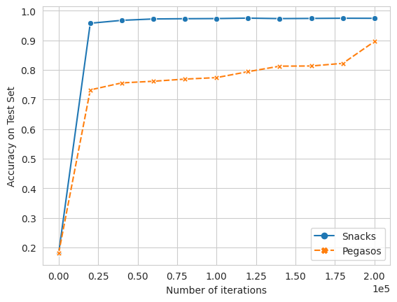
Figure 1: Accuracy on test set versus number of iterations

On this dataset, Snacks converges faster to the optimal value for the same number of iterations. Note that the cost of Pegasos and Snacks’ iterations are of similar magnitude (one call to the subgradient oracle and one Euclidean projection) and that the number of iterations for this experiment is significantly larger than during previous experiments (Snacks performs around $40000$ iterations on this dataset).

III-E Robustness of Snacks

Finally, we check the robustness of Snacks against variations of its main hyperparameters. The heatmap shown here is obtained for the a9a data set. We show how for different choices for the regularization parameter $\lambda$ and for the size $m$ of the random subspace Snacks is relatively robust, as it obtains similar results on a large region around the best values of $m$ and $\lambda$.

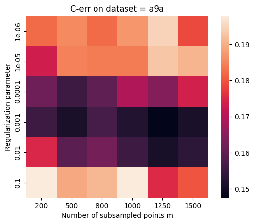
Figure 2: Classification error on test set vs $(m,\lambda)$

IV Conclusion

In this paper, we propose a kernel SVM solver called ”Snacks” which performs fast classification on huge scale datasets. The proposed method relies on two key points: reducing the computational burden by solving a Nyström approximation of the original problem and using an accelerated version of the stochastic subgradient method commonly used for kernel SVM solvers.

Numerical experiments support this claim and show a considerable speedup in training time compared to some state-of-the-art SVM solvers.

Further developments are possible, for example: evaluating Snacks on L1-SVM, providing statistical guarantees (based on [25]) for both uniform sampling and Approximate Leverage Scores (ALS) sampling, extending the library for multiclass classification using one-vs-all (OvA) or all-vs-all (AvA) scenarios. We defer these extensions for future work, hoping the Snacks toolbox will benefit practicioners.

References

- [1] James, G., Witten, D., Hastie, T. & Tibshirani, R. An introduction to statistical learning. (Springer,2013)
- [2] Schölkopf, B., Smola, A., Bach, F. & Others Learning with kernels: support vector machines, regularization, optimization, and beyond. (MIT press,2002)
- [3] Shawe-Taylor, J., Cristianini, N. & Others Kernel methods for pattern analysis. (Cambridge university press,2004)
- [4] Yang, M. Face recognition using kernel methods. Advances In Neural Information Processing Systems. 14 (2001)
- [5] Aronszajn, N. Theory of reproducing kernels. Transactions Of The American Mathematical Society. 68, 337-404 (1950)
- [6] Platt, J. Sequential minimal optimization: A fast algorithm for training support vector machines. (1998)
- [7] Schölkopf, B., Herbrich, R. & Smola, A. A generalized representer theorem. International Conference On Computational Learning Theory. pp. 416-426 (2001)
- [8] Rudi, A., Camoriano, R. & Rosasco, L. Less is More: Nyström Computational Regularization. Advances In Neural Information Processing Systems. 28 (2015)
- [9] Rudi, A. & Rosasco, L. Generalization Properties of Learning with Random Features. Advances In Neural Information Processing Systems. 30 (2017)
- [10] Rudi, A., Carratino, L. & Rosasco, L. FALKON: An Optimal Large Scale Kernel Method. Advances In Neural Information Processing Systems. 30 (2017)
- [11] Calandriello, D. & Rosasco, L. Statistical and computational trade-offs in kernel k-means. Advances In Neural Information Processing Systems. 31 (2018)
- [12] Steinwart, I. & Thomann, P. liquidSVM: A fast and versatile SVM package. ArXiv Preprint ArXiv:1702.06899. (2017)
- [13] Steinwart, I. & Christmann, A. Support vector machines. (Springer Science & Business Media,2008)
- [14] Kim, H., Howland, P., Park, H. & Christianini, N. Dimension reduction in text classification with support vector machines.. Journal Of Machine Learning Research. 6 (2005)
- [15] Pedregosa, F., Varoquaux, G., Gramfort, A., Michel, V., Thirion, B., Grisel, O., Blondel, M., Prettenhofer, P., Weiss, R., Dubourg, V. & Others Scikit-learn: Machine learning in Python. The Journal Of Machine Learning Research. 12 pp. 2825-2830 (2011)
- [16] Ding, C. & Dubchak, I. Multi-class protein fold recognition using support vector machines and neural networks. Bioinformatics. 17, 349-358 (2001)
- [17] Shalev-Shwartz, S., Singer, Y., Srebro, N. & Cotter, A. Pegasos: Primal estimated sub-gradient solver for svm. Mathematical Programming. 127, 3-30 (2011)
- [18] Chang, C. & Lin, C. LIBSVM: a library for support vector machines. ACM Transactions On Intelligent Systems And Technology (TIST). 2, 1-27 (2011)
- [19] Bottou, L. & Lin, C. Support vector machine solvers. Large Scale Kernel Machines. 3, 301-320 (2007)
- [20] Wen, Z., Shi, J., Li, Q., He, B. & Chen, J. ThunderSVM: A fast SVM library on GPUs and CPUs. The Journal Of Machine Learning Research. 19, 797-801 (2018)
- [21] Sun, Y., Gilbert, A. & Tewari, A. But How Does It Work in Theory? Linear SVM with Random Features. Advances In Neural Information Processing Systems. 31 (2018)
- [22] Li, Z., Ton, J., Oglic, D. & Sejdinovic, D. Towards a unified analysis of random Fourier features. International Conference On Machine Learning. pp. 3905-3914 (2019)
- [23] Williams, C. & Seeger, M. Using the Nyström method to speed up kernel machines. Advances In Neural Information Processing Systems. 13 (2000)
- [24] Yang, T., Li, Y., Mahdavi, M., Jin, R. & Zhou, Z. Nyström method vs random fourier features: A theoretical and empirical comparison. Advances In Neural Information Processing Systems. 25 (2012)
- [25] Della Vecchia, A., Mourtada, J., De Vito, E. & Rosasco, L. Regularized ERM on random subspaces. International Conference On Artificial Intelligence And Statistics. pp. 4006-4014 (2021)
- [26] Fan, R., Chang, K., Hsieh, C., Wang, X. & Lin, C. LIBLINEAR: A library for large linear classification. The Journal Of Machine Learning Research. 9 pp. 1871-1874 (2008)
- [27] Joachims, T. Training linear SVMs in linear time. Proceedings Of The 12th ACM SIGKDD International Conference On Knowledge Discovery And Data Mining. pp. 217-226 (2006)
- [28] Meanti, G., Carratino, L., Rosasco, L. & Rudi, A. Kernel methods through the roof: handling billions of points efficiently. Advances In Neural Information Processing Systems. 33 pp. 14410-14422 (2020)
- [29] Carratino, L., Vigogna, S., Calandriello, D. & Rosasco, L. Park: Sound and efficient kernel ridge regression by feature space partitions. Advances In Neural Information Processing Systems. 34 (2021)
- [30] Xu, Y., Lin, Q. & Yang, T. Accelerate stochastic subgradient method by leveraging local growth condition. Analysis And Applications. 17, 773-818 (2019)
- [31] Hsieh, C., Chang, K., Lin, C., Keerthi, S. & Sundararajan, S. A dual coordinate descent method for large-scale linear SVM. Proceedings Of The 25th International Conference On Machine Learning. pp. 408-415 (2008)
- [32] D’Aspremont, A., Scieur, D. & Taylor, A. Acceleration Methods. Foundations And Trends® In Optimization. 5, 1-245 (2021)
- [33] Rudi, A., Calandriello, D., Carratino, L. & Rosasco, L. On fast leverage score sampling and optimal learning. Advances In Neural Information Processing Systems. 31 (2018)