Frequency Regularization: Reducing Information Redundancy in Convolutional Neural Networks

Abstract.

Convolutional neural networks have demonstrated impressive results in many computer vision tasks. However, the increasing size of these networks raises concerns about the information overload resulting from the large number of network parameters. In this paper, we propose Frequency Regularization to restrict the non-zero elements of the network parameters in the frequency domain. The proposed approach operates at the tensor level, and can be applied to almost all network architectures. Specifically, the tensors of parameters are maintained in the frequency domain, where high frequency components can be eliminated by zigzag setting tensor elements to zero. Then, the inverse discrete cosine transform (IDCT) is used to reconstruct the spatial tensors for matrix operations during network training. Since high frequency components of images are known to be less critical, a large proportion of these parameters can be set to zero when networks are trained with the proposed frequency regularization. Comprehensive evaluations on various state-of-the-art network architectures, including LeNet, Alexnet, VGG, Resnet, ViT, UNet, GAN, and VAE, demonstrate the effectiveness of the proposed frequency regularization. For a very small accuracy decrease (less than 2%), a LeNet5 with 0.4M parameters can be represented by only 776 float16 numbers (over 1100$\times$ reduction), and a UNet with 34M parameters can be represented by only 759 float16 numbers (over 80000$\times$ reduction). In particular, the original size of the UNet model is 366MB, we reduce it to 4.5kb.

1. Introduction

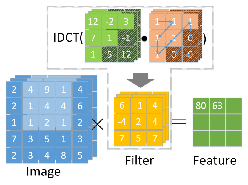
Figure 1. Illustration of the proposed frequency regularization. The tail elements of tensors in the frequency domain are truncated first, then input into the inverse of the discrete cosine transform to reconstruct the spatial tensor for learning features.

Convolutional neural networks have become increasingly popular in computer vision applications, such as image classification, image segmentation and so on. However, as the learning ability of these networks has improved, so has their size, growing from a few megabytes to hundreds of gigabytes (Dosovitskiy et al., 2021a). This leads to challenges such as enormous storage space or long transmission time on the Internet. After conducting a thorough literature review, we found that although larger networks tend to perform better, the accuracy improvement is not always directly proportional to the network size. In some cases, doubling the network size may not result in a significant accuracy improvement. From this observation we conclude that there may be information redundancy within various network architectures, leading to the question: “How can we reduce network information redundancy?”

It is commonly accepted that the performance of networks comes from the features learned by their parameters. For example, when a convolutional neural network such as Alexnet (Krizhevsky et al., 2017) is applied to an image classification task, the features learned by its convolutional kernels are closely related to the training images. Under this condition, features learned by a network are expected to have properties similar to the training images in which the high frequency components are known to be less important. Thus, it is reasonable to apply the frequency domain transforms, such as the discrete cosine transform, to the network parameters. Unfortunately, given the poor interpretability of complex network architectures, even a small change in a few key parameters can significantly affect the network performance. Based on this insight, the potential of frequency domain transforms for compressing or pruning networks may not be well-developed on pre-trained models, which has been the focus of previous approaches (Liu et al., 2018; Xu et al., 2020; Wang et al., 2016a, 2019). Instead, we focus on using the frequency domain transform as a network regularization to restrict information redundancy during the training process, and introduce Frequency Regularization (FR) as shown in Fig. 1.

The proposed frequency regularization can be divided into two steps: dynamic tail-truncation and inverse discrete cosine transform (IDCT). During network training, parameter tensors are maintained in the frequency domain, with the tail parts representing high frequency information zigzag truncated. The truncation process is implemented through a dot product with a zigzag mask matrix to ensure differentiability. After dynamic tail-truncation, tensors are input into the IDCT to reconstruct the spatial tensors that are then used as regular learning kernels in networks. Since the IDCT is a differentiable process, the actual tensors in the frequency domain can be updated through backpropagation algorithms. Moreover, as the reconstructed spatial tensors have the same size as those maintained in the frequency domain, the proposed frequency regularization can be easily applied to almost any type of network architecture. Furthermore, as features related to computer vision tasks are closely correlated to images, many parameters (from 90% to 99.99%) in the frequency domain can be set to 0 without an obvious decrease in network performance. The proposed frequency regularization has a few desirable properties:

• Generality: The proposed frequency regularization can be applied to almost any type of network architecture, as it is designed for tensors. Given this, we are able to evaluate the proposed frequency regularization on various state-of-the-art network architectures including LeNet, AlexNet, VGG, ResNet, ViT, UNet, GAN and VAE.

• Effectiveness: A large number of parameters can be truncated in the networks trained with the proposed frequency regularization, since it is widely recognized that high frequency information is unimportant for image data and the features learned by networks are closely correlated to images.

• Lossless property: There is no need to worry that the proposed frequency regularization will decrease network performance, since the inverse discrete cosine transform (IDCT) is usually considered as a lossless transformation. When no parameter is truncated, the proposed frequency regularization has almost no effect on the network performance.

2. related work

Frequency information has been widely used in convolutional neural networks for improving performance (Chen et al., 2020; Ciurana et al., 2019; Luo et al., 2022; Rhee et al., 2022; Saldanha et al., 2021; Shi et al., 2021; Ulicny et al., 2019; Wang et al., 2022b; Zhang et al., 2021; Zhao et al., 2022; Mi et al., 2022; Wang et al., 2022a; Zhou et al., 2022) pruning and network compression (Chen et al., 2023; Goldberg et al., 2020; Dziedzic et al., 2019; Shao et al., 2021; Wang et al., 2017; Xu et al., 2020; Wang et al., 2016a, 2019; Guyon et al., 2017; Hou et al., 2022; Lin et al., 2020; Li et al., 2017; Gao et al., 2022; Fang et al., 2023), or increasing the detection accuracy (Jia et al., 2022; Zhong et al., 2022; Shu et al., 2022). For instance, Wang et al. (Wang et al., 2022a) represented object edge and smooth structures using high and low frequency information, respectively. Mi et al. (Mi et al., 2022) split channel recognition networks into frequency domains, while Rippel et al. (Rippel et al., 2015) proposed a fully spectral representation of networks parameters. Buckler et al. (Buckler et al., 2021) introduced a similar idea with learnable parameters to determine the importance of different channels. Besides this, Han et al. (Han et al., 2016) compressed the networks with pruning, quantization and Huffman coding to achieve excellent results for network compression. Similarly, Wang et al. (Wang et al., 2016b, 2019) combined DCT, k-means, quantization and Huffman coding to compress the network parameters. Chen et al. (Chen et al., 2016) utilized DCT and hashing to assign high frequency to less hash buckets to achieve compression. Wang et al. (Dosovitskiy et al., 2021b) compress the vision transformer by removing the low-frequency components. Additionally, several works have proposed using the frequency representation of convolution kernels to prune less important channels (Lin et al., 2022; Zhang et al., 2023; Liu et al., 2018). Most of these previous works have primarily focused on the frequency domain representation of the input image, feature maps, or network parameters, but ignored the learning ability of the network parameters during training process. Since the network performance is usually sensitive to changes in a few key parameters, it cannot be guaranteed that these key parameters are located in the low frequency domain. As a result, these methods have only dropped 30% to 95% of parameters with minimal accuracy loss. In particular, although a few methods (Wang et al., 2019; Han et al., 2016) claimed around 50$\times$ of compression rate, but such rate is improved by quantization and entropy coding. The actual proportion of dropped parameters are still ranged from 30% to 95%. In contrast, the proposed frequency regularization approach restricts network parameters to the frequency domain, and high frequency elements are dynamically truncated during network training. This allows us to have much higher dropping rates of 90% to 99.99%.

The proposed frequency regularization approach is somewhat related to the DCT-Conv method proposed in (Chęiński and Wawrzyński, 2020), as both approaches maintain parameters in the frequency domain and utilized IDCT. However, there are several key differences between the two methods. First, the proposed frequency regularization can be applied to any layer with learnable parameters, including but not limited to convolution layers, fully connected layers, and transposed convolution layers. Therefore, we are able to evaluate the proposed frequency regularization on various of network architectures including Alexnet, VGG, Resnet, ViT, UNet, GAN and VAE. In contrast, DCT-Conv is a convolution layer with DCT, which are only evaluated on VGG and Resnet. Second, DCT-Conv randomly drops parameters in the frequency domain, which is not ideal since the components in low frequency and high frequency are considered as equally important. The ability to drop parameters of DCT-Conv is thus limited. Similar limitation is also shown in BA-FDNP method (Liu et al., 2018) in which the coefficients in frequency domain are used for pruning. Instead, in our approach, we truncate the tail parts of the parameters, as the high frequency components have been shown to be non-critical in features related to images. It is the most important difference between the proposed approach and these previous methods (Liu et al., 2018; Chęiński and Wawrzyński, 2020; Wang et al., 2019; Lin et al., 2022; Zhang et al., 2023) , and it is also the key that the proposed approach can achieve promising compression rate on various of network architectures.

3. Frequency Regularization and Tail-Truncation

When convolutional neural networks are applied to computer vision applications, the learned features are closely related to the training images. In fact, as shown by the visualized filters in AlexNet (Krizhevsky et al., 2017), the learned features actually look like real images. Based on this insight, it is reasonable to assume that the low frequency components of network parameters is more important than the high frequency components. Unfortunately, because of the poor interpretability of convolutional neural networks, a network’s performance may be highly sensitive to changes of the values in a few key parameters, which are not always located in the low frequency domain. This limits the proportion of dropped parameters in pre-trained models. Thus, we focus on restricting the number of non-zero parameters during the training process, and frequency regularization is thus proposed. It should be noted that network regularizations are typically introduced to prevent overfitting in neural networks (Goodfellow et al., 2016). In this paper, however, the definition of regularization is extended to include modifications or restrictions applied to networks with a particular purpose, such as restricting the number of non-zero parameters.

The idea behind the proposed frequency regularization is quite straightforward. Instead of maintaining the tensors of network parameters in the spatial domain, they are maintained in the frequency domain. This allows the tail elements of tensors to be truncated by a dot product with a zigzag mask matrix. During network training, the frequency tensors are input into the inverse discrete cosine transform (IDCT) to reconstruct the spatial tensors. Then, these spatial tensors are used as the regular learning kernels of convolutional neural networks for learning features. Since the IDCT process is differentiable, the parameters maintained in the frequency domain can be correctly updated during backpropagation. Moreover, as the IDCT can be used for tensors with any dimension without changing their size, the proposed frequency regularization can be implemented for any layer involving tensor operations, including convolution layers, fully connected layers, and transposed convolution layers. We first introduce the proposed frequency regularization for 1D tensors, and then discuss the implementation of regularization in higher dimensions.

Assume the 1D tensors of learning kernels to be $T(x)\in\mathbb{R}^{1\times D}$ where $x$ is the index. $T(x)$ represents the learnable parameters in the frequency domain which have been updated during training. $T(x)$ is first computed with a zigzag mask $\mathds{1}_{x<\epsilon}(x)$ for tail-truncation, then input into the IDCT to reconstruct the spatial tensor $W(y)\in\mathbb{R}^{1\times D}$ which can be the regular learning kernel in a 1D convolution layer. Mathematically:

(1) $$W(y) =\mathcal{F}_{\epsilon}(T(x))=\text{IDCT}\left(\bigcup_{x\in G_{x}}T(x)\cdot\mathds{1}_{x<\epsilon}(x)\right)$$

$$=\sum_{x\in G_{x}}T(x)\cdot\mathds{1}_{x<\epsilon}(x)\cdot\text{cos}\left[\frac{\pi}{D}\left(y+\frac{1}{2}\right)x\right]$$

$$=\sum_{x<\epsilon}T(x)\cdot\text{cos}\left[\frac{\pi}{D}\left(y+\frac{1}{2}\right)x\right],$$

where $x,y\in[0\ D\!\!-\!\!1]\cap\mathbb{N}=G_{x}$ are the indices of tensor $T(x)$ and $W(y)$ respectively. $T(X)$ is the actual tensor in the frequency domain and $W(y)$ is the corresponding reconstructed tensor in the spatial domain. $\text{IDCT}(\cdot)$ is the inverse discrete cosine transform. During the implementation, DCT-III which is the inverse of the widely used DCT-II is used. $\epsilon$ is the threshold value to control the truncation ratio. $\mathds{1}_{x<\epsilon}(x)$ is a binary mask to make the truncation process differentiable. Note that we removed the $\frac{T(0)}{2}$ in the above DCT-III since the learnable parameters can adaptively adjust this constant component.

Since the high dimensional IDCT can be decomposed into several 1D IDCTs, so high dimensional frequency regularization can also be expressed by several 1D frequency regularizations. Assume the two N-dimensional tensors in the frequency domain and spatial domain to be $T(\vec{x}),W(\vec{y})\in\mathbb{R}^{D_{1}\times D_{2},\cdots,D_{N}}$ where $\vec{x}=\{x_{1},x_{2},\cdots,x_{N}\}$ and $\vec{y}=\{y_{1},y_{2},\cdots,y_{N}\}$ are index vectors, $x_{i},y_{i}\in[0,D_{i}\!\!-\!\!1]\cap\mathbb{N}$. Then high dimensional frequency regularization $\mathcal{F}^{N}_{\epsilon}$ is:

(2) $$W(\vec{y}) =\mathcal{F}_{\epsilon}^{N}(T(\vec{x}))=\text{IDCT}^{N}\left(\bigcup_{\vec{x}\in G_{\vec{x}}}T(\vec{x})\cdot\mathds{1}_{|\vec{x}|_{1}<\epsilon}(\vec{x})\right)$$

$$=\sum_{\vec{x}\in G_{\vec{x}}}T(\vec{x})\cdot\mathds{1}_{|\vec{x}|_{1}<\epsilon}(\vec{x})\prod_{i=1}^{N}\text{cos}\left[\frac{\pi}{D_{i}}\left(y_{i}+\frac{1}{2}\right)x_{i}\right]$$

$$=\sum_{|\vec{x}|_{1}<\epsilon}T(\vec{x})\prod_{i=1}^{N}\text{cos}\left[\frac{\pi}{D_{i}}\left(y_{i}+\frac{1}{2}\right)x_{i}\right]$$

where $\text{IDCT}^{N}$ is the N-dimensional inverse discrete cosine transform, which can be easily implemented by N IDCTs in different dimensions. $\epsilon$ is the threshold value to control the truncation ratio. $|\vec{x}|_{1}=\sum_{x=1}^{N}|x_{i}|$ is the $L_{1}$ norm of the index vector $|\vec{x}|$. The indicator function $\mathds{1}_{|\vec{x}|_{1}<\epsilon}(\vec{x})$ is used to approximate the zigzag binary mask for truncating parameters.

Frequency regularization is proposed for tensors. Thus, it can be applied to any layer of a convolutional neural network, such as the convolution layer or fully connected layer. After applying the proposed frequency regularization, the formula of the convolution process can be re-expressed as:

(3) $$Z=WX+B\Rightarrow Z=\mathcal{F}_{\epsilon}^{N}(T_{W})X+\mathcal{F}_{\epsilon}(T_{B}),$$

where $T_{W}$ and $T_{B}$ are the tensors representing the weight and bias of the convolution layer. Usually, the size of the tensor in the convolution layer is 4D representing the number of kernels, input channel and kernel size. Based on the requirements of different applications, the proposed frequency can be 1D, 2D, 3D or 4D which can be controlled by users. In particular, the 4D frequency regularization gives us the highest compress rate, which has been used in the proposed evaluation experiments.

Table 1. Comparison between the proposed approach and DeepCompress(Han et al., 2016) on the MINIST dataset (LeCun et al., 1998).

	DeepCompress(Han et al., 2016)			DynSurgery (Guo et al., 2016) and BA-FDNP (Liu et al., 2018)			The Proposed Approach
	Top-1 Accuracy	Compress Rate	Number of Parameters	Top-1 Accuracy	Compress Rate	Number of Parameters	Top-1 Accuracy	Compress Rate	Number of Parameters
LeNet300-ref	98.36%	100%(1$\times$)	266K	97.72%	100%(1$\times$)	266K	98.15%	100%(1$\times$)	266K
LeNet300-v1	98.42%	2.5%(40$\times$)	21k(float6)	98.01 %	1.8%(56$\times$)	4.8k	97.11%	0.88%(114$\times$)	4238(float16)
LeNet300-v2							95.69%	0.53%(188$\times$)	2816(float16)
1-10 LeNet5-ref	99.20%	100%(1$\times$)	431K	99.09%	100%(1$\times$)	431K	98.78%	100%(1$\times$)	431K
LeNet5-v1	99.26%	2.56%(39$\times$)	34K(float6)	99.09%	0.92%(108$\times$)	4.0k	98.35%	0.89%(112$\times$)	7668(float16)
				BA-FDNP (Liu et al., 2018)			The proposed approach
5-10 LeNet5-v2				99.08%	0.67%(150$\times$)	2.8K	97.52%	0.09%(1110$\times$)	776(float16)

3.1. Dynamic tail-truncation:

According to the evaluation experiments we proposed in Section 4, usually over 99% of parameters in convolutional neural networks can be truncated without an obvious decrease in accuracy. However, there is also a serious issue that the remaining parameters may not have suitable gradients for backpropagation. In this condition, the training loss of the network restricted by the proposed frequency regularization sometimes may not change for hundreds of training epochs. This issue has occurred many times in our evaluation experiments. To address this problem, we propose the dynamic tail-truncation strategy. Instead of directly setting over 99% of the parameters to 0, this strategy continuously sets a few tail elements to 0 in every training epoch. In particular, as the total number of truncated parameters increases, the number of parameters truncated in each training epoch decreases. Mathematically, the ratio of truncated parameters is controlled by following function:

$$\beta_{n}=\beta_{n-1}-\gamma(\beta_{n-1}-\epsilon)$$

where $n$ is the index of training epoches. $\beta_{n-1},\beta_{n}\in[0,1]$ is the ratio of non-zeros parameters in epoch $n-1$ and $n$. $\gamma$ is the user parameter to control the speed of truncating parameters. During our evaluation experiment, $\gamma=0.01$ is used. $\epsilon$ is the user parameter to control the mininum ratio of non-zero parameters in the network. By changing the value of $\epsilon$, we can control the percentage of parameters that will be truncated in a network. For example, $\epsilon=0.01$ means that around $1-\epsilon=$ 99% of parameters will be truncated. Although the dynamic tail-truncation strategy requires extra training epochs, it results in a more stable training result when the minimum ratio $\epsilon$ is very small. This strategy has been used for all the evaluation experiments in this paper.

4. Experiments

In this section, we evaluate the proposed frequency regularization on several classical state-of-the-art network architectures including LeNet, Alexnet, VGG, ResNet, ViT, UNet, GAN and VAE on several standard datasets. During the evaluation, we first capture the accuracy of the original networks which is used as the reference accuracy to compare with the ones of networks restricted by the proposed frequency regularization. In particular, the implementation provided by authors or popular Github repositories are used. Then, these networks are re-trained with the proposed frequency regularization to compare the original networks. Since the parameters of networks are zigzag truncated in the proposed frequency regularization, we only need to save the location of the boundary between non-zero elements and zero elements as well as the size of tensors. Thus, the compress rate can be easily computed by dividing the number of non-zero parameters by the total number of parameters. Note that we did not consider the bias in the convolution layers, fully connected layers and transposed convolution layers during our evaluation, since the bias only represents a small portion of network parameters and most of the previous researchers also ignored them. Similarly, the parameters in batchnorm layers are also ignored with for same reason. Given the page limitation, we only demonstrate the total number of non-zero parameters in networks. More detailed are presented in the supplementary material. All the experiments are performed on GTX A4000 with 16 GB of video memory. The source code as well as our pre-trained model with frequency regularization will be made available following the acceptance of this paper.

Table 2. Evaluation of the proposed frequency regularization on Alexnet (Krizhevsky et al., 2017), VGG (Simonyan and Zisserman, 2015), ResNet (He et al., 2016) and ViT (Dosovitskiy et al., 2021b) using CIFAR10 dataset (Krizhevsky et al., 2009).

	Top-1 Accuracy	Compress Rate	Number of Parameters
AlexNet-ref	76.45 %	100%(1$\times$)	57,035,456
AlexNet-v1	77.44 %	1%(100$\times$)	570,365
AlexNet-v2	70.46 %	0.1%(1000$\times$)	57,364
AlexNet-v3	59.22 %	0.0025%(40509$\times$)	1,408
AlexNet-v4	58.55 %	0.00123%(81018$\times$)	1,408(float16)
1-4 VGG16-ref	85.84 %	100%(1$\times$)	20,024,000
VGG16-v1	84.77 %	1%(100$\times$)	200,578
VGG16-v2	73.01 %	0.1%(987$\times$)	20,302
VGG16-v3	65.99 %	0.0102%(9775$\times$)	2,048
1-4 ResNet18-ref	85.43 %	100%(1$\times$)	11,162,624
ResNet18-v1	85.34 %	1%(100$\times$)	111,901
ResNet18-v2	83.23 %	0.1%(1000$\times$)	12,058
ResNet18-v3	77.64 %	0.024%(4156$\times$)	2,688
1-4 ViT-ref	78.94 %	100%(1$\times$)	9,500,672
ViT-v1	78.98 %	9.77%(10$\times$)	928,478
ViT-v2	75.05 %	0.83%(120$\times$)	157,848(float16)

4.1. Comparison with state-of-the-art methods

To the best of our knowledge, there is no work which is directly related to the proposed approach on restricting the information redundancy during network training. The closest work we could find was proposed for network compression by pruning, such as DeepCompress (Han et al., 2016), DynSurgery (Guo et al., 2016) or BA-FDNP (Liu et al., 2018). Although there are a few newer methods proposed in (Wang et al., 2019; Luo et al., 2019; Chęiński and Wawrzyński, 2020; Ren et al., 2017; Fang et al., 2023; Hou et al., 2022; Lin et al., 2020; Liu et al., 2018), their advantage on compress rate is not very obvious and almost all of them work on networks pre-trained on large datasets. which makes the comparisons become very expensive considering computational resources. Besides, among all these previous approach, BA-FDNP (Liu et al., 2018) claimed the highest compress rate which is 150$\times$. Thus, we compare the proposed approach with DeepCompress (Han et al., 2016) ,DynSurgery (Guo et al., 2016) and BA-FDNP (Liu et al., 2018). The comparison results are shown in Table 1. In particular, the top-1 accuracy (Krizhevsky et al., 2017) is used as evaluation metric. The proposed approach achieves much higher compress rate without obvious decrease in top-1 accuracy. For example, in LeNet300-v1, the proposed approach achieves 112$\times$ the compress rate with less than 1% of cost in top1-accuracy. Furthermore, it achieves 1110 $\times$ compress rate in LeNet5-v2 with only 2% of top1-accuracy decrease, which is much higher than the DeepCompress (Han et al., 2016), DynSurgery (Guo et al., 2016), BA-FDNP (Liu et al., 2018) as well as those following works (Wang et al., 2019; Luo et al., 2019; Chęiński and Wawrzyński, 2020; Ren et al., 2017; Fang et al., 2023; Hou et al., 2022; Lin et al., 2020; Liu et al., 2018). It should be noted that the BA-FDNP (Liu et al., 2018) proposed to do pruning in frequency domain which is related to the proposed approach. However, as we mentioned in Section 2, instead of truncating the tail parts of tensor, BA-FDNP (Liu et al., 2018) utilized the coefficients matrix for pruning which limits their compress rate. As a result, BA-FDNP only has 150$\times$ compress rate on LeNet5-v2, but the proposed can achieve around 1110 $\times$ reduction with less than 2% of top-1 accuracy decrease. It should be noted that BA-FDNP (Liu et al., 2018) utilized data argumentation to improve top-1 accuracy. It also applied the pre-trained model for initialization and retrain their model for 20k iterations for searching the highest top-1 accuracy model, However, none of these techniques for accuracy improvement are applied in the proposed approach, with the consideration of our computation resource. Both LeNet300 and LeNet5 are quite simple architectures and the MINIST dataset is also not a very challenging dataset. In order to thoroughly evaluate the proposed approach, we further apply the proposed frequency regularization on various state-of-the-art network architectures in the remaining sections.

4.2. Image classification

Image classification has been studied for decades in computer vision. There are many excellent architectures that have been proposed in this field. Thus, we evaluate the performance of the proposed frequency regularization on Alexnet (Krizhevsky et al., 2017), VGG16 (Simonyan and Zisserman, 2015), ResNet18 (He et al., 2016) and ViT (Dosovitskiy et al., 2021b). During evaluation, the cifar10 dataset (Krizhevsky et al., 2009) is used for training and testing and top1-accuracy is used as the evaluation metric. Note that we did not apply tuning techniques or pre-trained model during evaluation considering training time. The accuracy scores can be higher once some training techniques such as dynamic learning rate or data argumentation is utilized, which has been widely used in previous approaches (Wang et al., 2019; Luo et al., 2019; Chęiński and Wawrzyński, 2020; Ren et al., 2017; Fang et al., 2023; Hou et al., 2022; Lin et al., 2020; Liu et al., 2018).

The evaluation results are shown in Table 2. AlexNet-ref which is the original Alexnet (Krizhevsky et al., 2017) achieves 76.45% top-1 accuracy. After 99% parameters have been truncated, AlexNet-v1 achieves 77.44% top-1 accuracy which is a little bit higher than the original one. This improvement comes from the fact that the tail-truncation can be considered as a regularization to prevent a network from overfitting just like the dropout layer. When only 0.1% of parameters are kept in the frequency domain, AlexNet-v2 has 70.46% in top-1 accuracy, and the compress rate becomes 1000$\times$. Furthermore, in the extreme case where only 1408 non-zero parameters are kept in AlexNet, AlexNet-v3 still achieves 59.22%. We also applied the network on the half float condition, and AlexNet-v4 consisting of 1408 float16 numbers achieves 58.55% with the compress rate increasing to 81018$\times$, which is a very interesting discovery. Similar results are also observed in VGG16 and ResNet18. In particular, ResNet18-v3 with only 2688 parameters achieves 77.64%, which is even higher than the original AlexNet-ref with 57M parameters. We also evaluate the proposed frequency regularization on ViT consist of self-attention layers which are actually not very suitable frequency domain transformation. Previous work (Wang et al., 2022b; Fang et al., 2023) related to transformer only achieves around 50% of pruning ratio. For the proposed approach, there is around 75% top-1 accuracy in ViT-v2 in which over 98% of parameters are truncated. But when only 90% of parameters are truncated, the ViT-v1 has no accuracy decrease, which demonstrate the generality of the proposed approach. The evaluation of proposed approach on these networks clearly demonstrates that the information redundancy inside networks can be restricted well by the proposed frequency regularization. However, the resolution of images in CIFAR10 is not very high, which may raise a concern that the proposed frequency regularization only works well on small images. Thus, we evaluated the proposed technique on UNet for high resolution image segmentation.

Table 3. Evaluation of the proposed frequency regularization on UNet for image segmentation tasks using Carvana Image Masking Challenge Dataset (Iglovikov and Shvets, 2018).

	Dice Score	Compress Rate	Number of Parameters
UNet-ref	99.13 %	100%(1$\times$)	31,043,586
UNet-v1	99.51 %	1%(100$\times$)	310,964
UNet-v2	99.37 %	0.1%(1000$\times$)	31,096
UNet-v3	98.86 %	0.0094%(10573$\times$)	2,936
1-4 UNet-v4	97.19 %	0.0012%(81801$\times$)	759(float16)

4.3. Image Segmentation

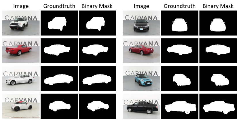
Figure 2. The segmentation results of UNet parameters restricted by the proposed frequency domain, with over 99.99% of parameters truncated, for the Carvana Image Masking Challenge Dataset (Iglovikov and Shvets, 2018).

After a comprehensive literature review, we found a limited number of methods focussing on prunning or compressing segmentation networks, even DepGraph (Fang et al., 2023), which is the latest prunning method proposed for any structural prunning, was not evaluated on segmentation networks. One reason maybe the sense that the information redundancy for segmentation networks should be lower than image classification networks. However, the proposed frequency regularization is supposed to work well on any features related to images and segmentation networks should be one of them. We thus evaluate the proposed frequency regularization on UNet using the Carvana Image Masking Challenge Dataset (Iglovikov and Shvets, 2018), which is a popular dataset for segmentation challenge in Kaggle competitions. In particular, the Dice Score is used for evaluation.

Table 4. Evaluation of the proposed frequency regularization on generative adversarial network (GAN) and variational autoencoder (VAE).

	Fid value	Compress Rate	Number of Parameters
GAN-ref	244	100%(1$\times$)	6,334,464
GAN-v1	248	1.02%(98 $\times$)	64,383
1-4 VAE-ref	81	100%(1$\times$)	971,200
VAE-v1	94	10%(10$\times$)	97,134

Actually, compared to image classification networks, UNet architecture usually consists of pure convolution layers with on bias which are more suitable for the proposed frequency regularization. As shown in Table 3, the orignal UNet containing 31M parameters achieves 99.31% Dice score. Once over 99% parameters have been truncated in the frequency domain, UNet-v1 achieves 99.51 % Dice score. Moreover, UNet-v3 achieves promising results with 98.86% in Dice score, in which only 2936 parameters are kept. Finally, we tested the proposed approach on the most extreme condition in which only 759 float16 parameters are kept in UNet-v4. In particular, we also disabled all the bias in the networks and learning parameters in batchnorm, which guaranteed the UNet-v4 only has 759 non-zero float16 parameters. Surprisingly, the UNet-v4 still achieves 97.19% in Dice score. This is an unbelievable result, a UNet with only 759 parameters can achieve around 97% in Dice score for the Carvana Image Masking Challenge Dataset. Note that there are over 5000 images with 959 $\times$ 460 resolution which is much higher than the resolutions of images in CIFAR10 (Krizhevsky et al., 2009). We double checked the non-zero parameters in every layer in UNet to make sure that this conclusion is correct, and the visualized segmentation mask is shown in Fig. 2. We also include this pre-train UNet into the supplementary materials as well as a few testing images. The original size of the UNet model exceeds 366MB, but our frequency regularization technique reduces it to 40kb. Additionally, using an entropy compression tool on Ubuntu, we further reduce the size to 4.5kb.

GAN-ref: 244 Fid value

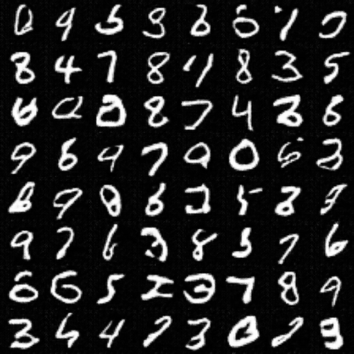
GAN-v1: 248 Fid value

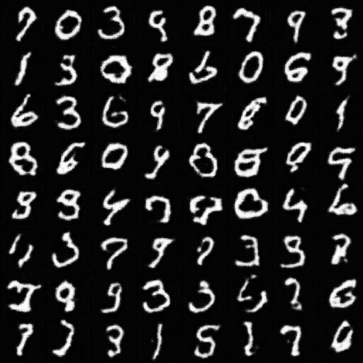
Figure 3. Comparisons between images generated by the orignal GAN network and GAN with our frequency regularization in which over 99% of parameters are truncated.

4.4. Image Generation

Compare to classification or segmentation networks, image generation networks such as the generative adversarial network (GAN) or variational autoencoder (VAE) are not very suitable for the proposed frequency regularization, since what has been learned by these networks are claimed as distribution information. However, these distributions are still related to images. Thus, we also evaluate the proposed approach on generative adversarial network and varitional autoencoder. Since both networks usually require long time for training, we used the MINIST dataset for evaluation and the Fid value (Wang et al., 2016a) is used as the evaluation metric. As shown in Table 4, the proposed approach achieves similar results when 99% of the parameters are truncated compared to the orignal GAN network. The generated images are also demonstrated in Fig. 3, where the images generated by GAN with the proposed frequency are similar to the original GAN. We also evaluate the proposed approach regularization on VAE. Since the VAE we used is the simplest version in which there are only two fully connected layers in their encoder and three fully connected layers in their decoder, we only truncate 90% of the parameters for VAE. The visual results are shown in Fig. 4. During the training of VAE and GAN, with or without the proposed frequency regularization, we stop the training once the visual results look good. Actually, with more training epoches, the quality of the generated images can be better.

VAE-ref: 81 Fid value

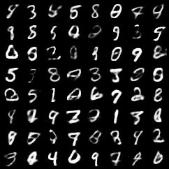
VAE-v1: 94 Fid value

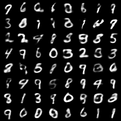
Figure 4. Comparisons between images generated by the orignal VAE network and VAE with our frequency regularization in which over 90% of the parameters are truncated.

4.5. Limitation and Future Work

The proposed frequency regularization is based on the assumption that the high frequency component is unimportant. This may not work well on the tensors of parameters which are not related to images. This disadvatange can be seen for the comparison between evaluations on image segmentation in Section 4.3 and image generation in Section 4.4, where the parameters in the generation networks cannot be truncated too much. In addition, although the parameter of the proposed approach is in the frequency domain, it still needs to be converted into the spatial domain for convolution operations. This leads to an extra memory cost during networks training. However, once the networks have been well-trained, a high compress rate can be achieved which is very useful for network transmission on the Internet. The memory cost does not exist during testing, since the networks need to be unpacked only once. Since around 99% of the parameters in networks restricted by the proposed frequency regularization can be truncated, it is very much possible to speed-up the network inference. This will be the next direction of our research.

5. Conclusion

In this paper we proposed frequency regularization to restrict the information redundancy of convolutional neural networks devised for computer vision tasks. The proposed regularization maintains the tensors of parameters in the frequency domain where the high frequency component can be truncated. During training, the tail part of tensors are truncated first before being input into the inverse discrete cosine transform to reconstruct the spatial tensors that are used for tensor operations. In particular, the dynamic tail-truncation strategy was proposed to improve the stability of network training. We applied the proposed frequency regularization in various state-of-the-art network architectures for evaluation. Comprehensive experiments demonstrated that between 90% to 99.99% of the parameters in the frequency domain can be truncated. This demonstrates the promising ability of the proposed frequency regularization to restrict the information redundancy in convolutional neural networks for computer vision tasks.

References

- (1)
- Buckler et al. (2021) Mark Buckler, Neil Adit, Yuwei Hu, Zhiru Zhang, and Adrian Sampson. 2021. Dense Pruning of Pointwise Convolutions in the Frequency Domain. arXiv preprint arXiv:2109.07707 (2021). arXiv:2109.07707
- Chen et al. (2020) Hanting Chen, Yunhe Wang, Han Shu, Yehui Tang, Chunjing Xu, Boxin Shi, Chao Xu, Qi Tian, and Chang Xu. 2020. Frequency Domain Compact 3d Convolutional Neural Networks. In Proceedings of the IEEE/CVF Conference on Computer Vision and Pattern Recognition. 1641–1650.
- Chen et al. (2016) Wenlin Chen, James Wilson, Stephen Tyree, Kilian Q Weinberger, and Yixin Chen. 2016. Compressing Convolutional Neural Networks in the Frequency Domain. In Proceedings of the 22nd ACM SIGKDD International Conference on Knowledge Discovery and Data Mining. 1475–1484.
- Chen et al. (2023) Yaosen Chen, Renshuang Zhou, Bing Guo, Yan Shen, Wei Wang, Xuming Wen, and Xinhua Suo. 2023. Discrete Cosine Transform for Filter Pruning. Applied Intelligence 53, 3 (2023), 3398–3414.
- Chęiński and Wawrzyński (2020) Karol Chęiński and Paweł Wawrzyński. 2020. DCT-Conv: Coding filters in convolutional networks with Discrete Cosine Transform. In 2020 International Joint Conference on Neural Networks (IJCNN). 1–6. https://doi.org/10.1109/IJCNN48605.2020.9207103
- Ciurana et al. (2019) Adrià Ciurana, Albert Mosella-Montoro, and Javier Ruiz-Hidalgo. 2019. Hybrid Cosine Based Convolutional Neural Networks. arXiv preprint arXiv:1904.01987 (2019). arXiv:1904.01987
- Dosovitskiy et al. (2021a) Alexey Dosovitskiy, Lucas Beyer, Alexander Kolesnikov, Dirk Weissenborn, Xiaohua Zhai, Thomas Unterthiner, Mostafa Dehghani, Matthias Minderer, Georg Heigold, Sylvain Gelly, Jakob Uszkoreit, and Neil Houlsby. 2021a. An Image is Worth 16x16 Words: Transformers for Image Recognition at Scale. In International Conference on Learning Representations. https://openreview.net/forum?id=YicbFdNTTy
- Dosovitskiy et al. (2021b) Alexey Dosovitskiy, Lucas Beyer, Alexander Kolesnikov, Dirk Weissenborn, Xiaohua Zhai, Thomas Unterthiner, Mostafa Dehghani, Matthias Minderer, Georg Heigold, Sylvain Gelly, Jakob Uszkoreit, and Neil Houlsby. 2021b. An Image is Worth 16x16 Words: Transformers for Image Recognition at Scale. In International Conference on Learning Representations. https://openreview.net/forum?id=YicbFdNTTy
- Dziedzic et al. (2019) Adam Dziedzic, John Paparrizos, Sanjay Krishnan, Aaron Elmore, and Michael Franklin. 2019. Band-Limited Training and Inference for Convolutional Neural Networks. In International Conference on Machine Learning. PMLR, 1745–1754.
- Fang et al. (2023) Gongfan Fang, Xinyin Ma, Mingli Song, Michael Bi Mi, and Xinchao Wang. 2023. DepGraph: Towards Any Structural Pruning. In Proceedings of the IEEE/CVF Conference on Computer Vision and Pattern Recognition.
- Gao et al. (2022) Shangqian Gao, Feihu Huang, Yanfu Zhang, and Heng Huang. 2022. Disentangled differentiable network pruning. In Computer Vision–ECCV 2022: 17th European Conference, Tel Aviv, Israel, October 23–27, 2022, Proceedings, Part XI. Springer, 328–345.
- Goldberg et al. (2020) Kfir Goldberg, Stav Shapiro, Elad Richardson, and Shai Avidan. 2020. Rethinking Fun: Frequency-domain Utilization Networks. arXiv preprint arXiv:2012.03357 (2020). arXiv:2012.03357
- Goodfellow et al. (2016) Ian Goodfellow, Yoshua Bengio, and Aaron Courville. 2016. Deep learning. MIT press.
- Guo et al. (2016) Yiwen Guo, Anbang Yao, and Yurong Chen. 2016. Dynamic network surgery for efficient dnns. Advances in neural information processing systems 29 (2016).
- Guyon et al. (2017) I. Guyon, U. Von Luxburg, S. Bengio, H. Wallach, R. Fergus, S. Vishwanathan, and R. Garnett (Eds.). 2017. GANs Trained by a Two Time-Scale Update Rule Converge to a Local Nash Equilibrium. Vol. 30. Curran Associates, Inc. https://proceedings.neurips.cc/paper_files/paper/2017/file/8a1d694707eb0fefe65871369074926d-Paper.pdf
- Han et al. (2016) Song Han, Huizi Mao, and William J. Dally. 2016. Deep Compression: Compressing Deep Neural Network with Pruning, Trained Quantization and Huffman Coding. In 4th International Conference on Learning Representations, ICLR 2016, San Juan, Puerto Rico, May 2-4, 2016, Conference Track Proceedings, Yoshua Bengio and Yann LeCun (Eds.). http://arxiv.org/abs/1510.00149
- He et al. (2016) Kaiming He, Xiangyu Zhang, Shaoqing Ren, and Jian Sun. 2016. Deep residual learning for image recognition. In Proceedings of the IEEE conference on computer vision and pattern recognition. 770–778.
- Hou et al. (2022) Zejiang Hou, Minghai Qin, Fei Sun, Xiaolong Ma, Kun Yuan, Yi Xu, Yen-Kuang Chen, Rong Jin, Yuan Xie, and Sun-Yuan Kung. 2022. Chex: channel exploration for CNN model compression. In Proceedings of the IEEE/CVF Conference on Computer Vision and Pattern Recognition. 12287–12298.
- Iglovikov and Shvets (2018) Vladimir Iglovikov and Alexey Shvets. 2018. Ternausnet: U-net with vgg11 encoder pre-trained on imagenet for image segmentation. arXiv preprint arXiv:1801.05746 (2018).
- Jia et al. (2022) Shuai Jia, Chao Ma, Taiping Yao, Bangjie Yin, Shouhong Ding, and Xiaokang Yang. 2022. Exploring Frequency Adversarial Attacks for Face Forgery Detection. In Proceedings of the IEEE/CVF Conference on Computer Vision and Pattern Recognition. 4103–4112.
- Krizhevsky et al. (2009) Alex Krizhevsky, Geoffrey Hinton, et al. 2009. Learning multiple layers of features from tiny images. (2009).
- Krizhevsky et al. (2017) Alex Krizhevsky, Ilya Sutskever, and Geoffrey E. Hinton. 2017. ImageNet Classification with Deep Convolutional Neural Networks. Commun. ACM 60, 6 (may 2017), 84–90. https://doi.org/10.1145/3065386
- LeCun et al. (1998) Yann LeCun, Léon Bottou, Yoshua Bengio, and Patrick Haffner. 1998. Gradient-based learning applied to document recognition. Proc. IEEE 86, 11 (1998), 2278–2324.
- Li et al. (2017) Hao Li, Asim Kadav, Igor Durdanovic, Hanan Samet, and Hans Peter Graf. 2017. Pruning filters for efficient convnets. (2017).
- Lin et al. (2020) Mingbao Lin, Rongrong Ji, Yan Wang, Yichen Zhang, Baochang Zhang, Yonghong Tian, and Ling Shao. 2020. Hrank: Filter pruning using high-rank feature map. In Proceedings of the IEEE/CVF conference on computer vision and pattern recognition. 1529–1538.
- Lin et al. (2022) Rui Lin, Jie Ran, Dongpeng Wang, King Hung Chiu, and Ngai Wong. 2022. EZCrop: Energy-Zoned Channels for Robust Output Pruning. In Proceedings of the IEEE/CVF Winter Conference on Applications of Computer Vision. 19–28.
- Liu et al. (2018) Zhenhua Liu, Jizheng Xu, Xiulian Peng, and Ruiqin Xiong. 2018. Frequency-Domain Dynamic Pruning for Convolutional Neural Networks. Advances in neural information processing systems 31 (2018).
- Luo et al. (2022) Cheng Luo, Qinliang Lin, Weicheng Xie, Bizhu Wu, Jinheng Xie, and Linlin Shen. 2022. Frequency-Driven Imperceptible Adversarial Attack on Semantic Similarity. In Proceedings of the IEEE/CVF Conference on Computer Vision and Pattern Recognition. 15315–15324.
- Luo et al. (2019) Jian-Hao Luo, Hao Zhang, Hong-Yu Zhou, Chen-Wei Xie, Jianxin Wu, and Weiyao Lin. 2019. ThiNet: Pruning CNN Filters for a Thinner Net. IEEE Transactions on Pattern Analysis and Machine Intelligence 41, 10 (2019), 2525–2538. https://doi.org/10.1109/TPAMI.2018.2858232
- Mi et al. (2022) Yuxi Mi, Yuge Huang, Jiazhen Ji, Hongquan Liu, Xingkun Xu, Shouhong Ding, and Shuigeng Zhou. 2022. DuetFace: Collaborative Privacy-Preserving Face Recognition via Channel Splitting in the Frequency Domain. In Proceedings of the 30th ACM International Conference on Multimedia (Lisboa, Portugal) (MM ’22). Association for Computing Machinery, New York, NY, USA, 6755–6764. https://doi.org/10.1145/3503161.3548303
- Ren et al. (2017) Shaoqing Ren, Kaiming He, Ross Girshick, Xiangyu Zhang, and Jian Sun. 2017. Object Detection Networks on Convolutional Feature Maps. IEEE Transactions on Pattern Analysis and Machine Intelligence 39, 7 (2017), 1476–1481. https://doi.org/10.1109/TPAMI.2016.2601099
- Rhee et al. (2022) Hochang Rhee, Yeong Il Jang, Seyun Kim, and Nam Ik Cho. 2022. LC-FDNet: Learned Lossless Image Compression with Frequency Decomposition Network. In Proceedings of the IEEE/CVF Conference on Computer Vision and Pattern Recognition. 6033–6042.
- Rippel et al. (2015) Oren Rippel, Jasper Snoek, and Ryan P Adams. 2015. Spectral Representations for Convolutional Neural Networks. Advances in neural information processing systems 28 (2015).
- Saldanha et al. (2021) Nikhil Saldanha, Silvia L Pintea, Jan C van Gemert, and Nergis Tomen. 2021. Frequency Learning for Structured CNN Filters with Gaussian Fractional Derivatives. arXiv preprint arXiv:2111.06660 (2021). arXiv:2111.06660
- Shao et al. (2021) Zhuang Shao, Xiaoliang Chen, Li Du, Lei Chen, Yuan Du, Wei Zhuang, Huadong Wei, Chenjia Xie, and Zhongfeng Wang. 2021. Memory-Efficient CNN Accelerator Based on Interlayer Feature Map Compression. IEEE Transactions on Circuits and Systems I: Regular Papers 69, 2 (2021), 668–681.
- Shi et al. (2021) Yubo Shi, Meiqi Wang, Siyi Chen, Jinghe Wei, and Zhongfeng Wang. 2021. Transform-Based Feature Map Compression for Cnn Inference. In 2021 IEEE International Symposium on Circuits and Systems (ISCAS). IEEE, 1–5.
- Shu et al. (2022) Weibo Shu, Jia Wan, Kay Chen Tan, Sam Kwong, and Antoni B Chan. 2022. Crowd Counting in the Frequency Domain. In Proceedings of the IEEE/CVF Conference on Computer Vision and Pattern Recognition. 19618–19627.
- Simonyan and Zisserman (2015) Karen Simonyan and Andrew Zisserman. 2015. Very Deep Convolutional Networks for Large-Scale Image Recognition. In International Conference on Learning Representations.
- Ulicny et al. (2019) Matej Ulicny, Vladimir A Krylov, and Rozenn Dahyot. 2019. Harmonic Networks for Image Classification. In British Machine Vision Conference (BMVC). British Machine Vision Association.
- Wang et al. (2022a) Jingye Wang, Ruoyi Du, Dongliang Chang, Kongming Liang, and Zhanyu Ma. 2022a. Domain Generalization via Frequency-Domain-Based Feature Disentanglement and Interaction. In Proceedings of the 30th ACM International Conference on Multimedia (Lisboa, Portugal) (MM ’22). Association for Computing Machinery, New York, NY, USA, 4821–4829. https://doi.org/10.1145/3503161.3548267
- Wang et al. (2017) Yunhe Wang, Chang Xu, Chao Xu, and Dacheng Tao. 2017. Beyond Filters: Compact Feature Map for Portable Deep Model. In International Conference on Machine Learning. PMLR, 3703–3711.
- Wang et al. (2019) Yunhe Wang, Chang Xu, Chao Xu, and Dacheng Tao. 2019. Packing Convolutional Neural Networks in the Frequency Domain. IEEE Transactions on Pattern Analysis and Machine Intelligence 41, 10 (2019), 2495–2510. https://doi.org/10.1109/TPAMI.2018.2857824
- Wang et al. (2016a) Yunhe Wang, Chang Xu, Shan You, Dacheng Tao, and Chao Xu. 2016a. CNNpack: Packing Convolutional Neural Networks in the Frequency Domain. In Advances in Neural Information Processing Systems, D. Lee, M. Sugiyama, U. Luxburg, I. Guyon, and R. Garnett (Eds.), Vol. 29. Curran Associates, Inc. https://proceedings.neurips.cc/paper_files/paper/2016/file/3636638817772e42b59d74cff571fbb3-Paper.pdf
- Wang et al. (2016b) Yunhe Wang, Chang Xu, Shan You, Dacheng Tao, and Chao Xu. 2016b. Cnnpack: Packing Convolutional Neural Networks in the Frequency Domain. Advances in neural information processing systems 29 (2016).
- Wang et al. (2022b) Zhenyu Wang, Hao Luo, Pichao Wang, Feng Ding, Fan Wang, and Hao Li. 2022b. VTC-LFC: Vision Transformer Compression with Low-Frequency Components. Advances in Neural Information Processing Systems 35 (Dec. 2022), 13974–13988.
- Xu et al. (2020) K. Xu, M. Qin, F. Sun, Y. Wang, Y. Chen, and F. Ren. 2020. Learning in the Frequency Domain. In 2020 IEEE/CVF Conference on Computer Vision and Pattern Recognition (CVPR). IEEE Computer Society, Los Alamitos, CA, USA, 1737–1746. https://doi.org/10.1109/CVPR42600.2020.00181
- Zhang et al. (2021) Chen Zhang, Yinghao Xu, and Yujun Shen. 2021. Compconv: A Compact Convolution Module for Efficient Feature Learning. In Proceedings of the IEEE/CVF Conference on Computer Vision and Pattern Recognition. 3012–3021.
- Zhang et al. (2023) Shuo Zhang, Mingqi Gao, Qiang Ni, and Jungong Han. 2023. Filter Pruning with Uniqueness Mechanism in the Frequency Domain for Efficient Neural Networks. Neurocomputing 530 (2023), 116–124.
- Zhao et al. (2022) Tiesong Zhao, Weize Feng, HongJi Zeng, Yiwen Xu, Yuzhen Niu, and Jiaying Liu. 2022. Learning-Based Video Coding with Joint Deep Compression and Enhancement. In Proceedings of the 30th ACM International Conference on Multimedia (Lisboa, Portugal) (MM ’22). Association for Computing Machinery, New York, NY, USA, 3045–3054. https://doi.org/10.1145/3503161.3548314
- Zhong et al. (2022) Yijie Zhong, Bo Li, Lv Tang, Senyun Kuang, Shuang Wu, and Shouhong Ding. 2022. Detecting Camouflaged Object in Frequency Domain. In Proceedings of the IEEE/CVF Conference on Computer Vision and Pattern Recognition. 4504–4513.
- Zhou et al. (2022) Man Zhou, Jie Huang, Chongyi Li, Hu Yu, Keyu Yan, Naishan Zheng, and Feng Zhao. 2022. Adaptively Learning Low-High Frequency Information Integration for Pan-Sharpening. In Proceedings of the 30th ACM International Conference on Multimedia (Lisboa, Portugal) (MM ’22). Association for Computing Machinery, New York, NY, USA, 3375–3384. https://doi.org/10.1145/3503161.3547924