Iterative projection method for unsteady Navier-Stokes equations with high Reynolds numbers

Abstract

A new approach, iteration projection method, is proposed to solve the saddle point problem obtained after the full discretization of the unsteady Navier-Stokes equations. It is motivated by the Uzawa method, an iterative method for saddle point problems, and the convectional projection method for the Navier-Stokes equations that projects the intermediate velocity to the divergence free space only once per time step. The proposed method iterates projections in each time step with a proper convection form. We prove that the projection iterations converge with a certain parameter regime. Optimal iteration convergence can be achieved with the modulation of parameter values.

This new method has several significant improvements over the Uzawa method and the projection method both theoretically and practically. First, when the iterative projections are fully convergent in each time step, the numerical velocity is weakly divergence free (pointwise divergence free in divergence free finite element methods), and the stability and error estimate are rigorously proven. With proper parameters, this method converges much faster than the Uzawa method. Second, numerical simulations show that with rather relaxed stopping criteria which require only a few iterations each time step, the numerical solution preserves stability and accuracy for high Reynolds numbers, where the convectional projection method would fail. Furthermore, this method retains the efficiency of the traditional projection method by decoupling the velocity and pressure fields, which splits the saddle point system into small elliptic problems. Three dimensional simulations with Taylor-Hood P2/P1 finite elements are presented to demonstrate the performance and efficiency of this method.

More importantly, this method is a generic approach and thus there are many potential improvements and extensions of the iterative projection method, including utilization of various convection forms, association with stabilization techniques for high Reynolds numbers, applications to other saddle point problems.

Keywords. Navier-Stokes equations, iterative projection method, saddle-point problems, divergence free velocity, skew-symmetric convection, fully implicit scheme

1 Introduction

1.1 Problem and motivation

The incompressible Navier-Stokes equations are predominant in viscous fluid dynamics, including problems with high Reynolds numbers such as turbulence flows. However, it is extremely challenging to design efficient and robust numerical schemes for these problems. A major difficulty is the treatment of the incompressibility constraint, or the divergence free condition, which couples the velocity and pressure. Consider a bounded three-dimensional domain $\Omega$ and the Navier-Stokes equations

$${u}_{t}-\nu\Delta u+\text{NL}(u,u)+\nabla p =f,$$ (1)

$$\nabla\cdot{u} =0,$$ (2)

with the nonlinear convection $\text{NL}(u,u)=(u\cdot\nabla)u$, the Dirichlet boundary condition $u|_{\partial\Omega}=0$, where $u=(u_{1},u_{2},u_{3})$ is the velocity, $p$ is the kinematic pressure, $\nu$ is the kinematic viscosity, and $f$ is the force. There are various equivalent forms of the convection term (e.g., see [9]), and this work focuses on the skew-symmetric form

$$\text{NL}(u,v)=(u\cdot\nabla)v+\frac{1}{2}(\nabla\cdot u)v.$$ (3)

It is well-known that this form can be used to prove the stability of finite element methods for Navier-Stokes equations (see e.g., [14, Theorem 4.3]). This work adopts the popular BDF2 (Backward Differentiation Formula 2) time integration for Navier-Stokes equations. Let $k>0$ be the uniform time step size. Denote the numerical solutions of velocity and pressure at time step $t_{n}=nk$ as ${u}^{n}$ and $p^{n}$, respectively. One obtains the following scheme,

$$(1.5-k\nu\Delta)u^{n+1}+k\text{NL}(\tilde{w},u^{n+1})+k\nabla p^{n+1} =F^{n+1},$$ (4)

$$\nabla\cdot u^{n+1} =0,$$ (5)

where $F^{n+1}=2{u}^{n}-0.5{u}^{n-1}+kf^{n+1}$. The choice of $\tilde{w}$ leads to two different problems.

• When $\tilde{w}=w^{n+1}\triangleq 2{u}^{n}-{u}^{n-1}$, a second order extrapolation of $u^{n+1}$, the convection term is semi-implicit. Then, a spatial discretization of this scheme using, e.g., the mixed finite elements methods yields a generalized saddle point problem (see Remark 1). Some extensive studies of the solvers of the saddle point problems can be found in [5, 1].

• When $\tilde{w}=u^{n+1}$, the convection term is fully implicit and this scheme is nonlinear. Typically, a nonlinear solver such as the Picard or Newton method is employed to linearize it to a series of saddle point problems, which are then computed by saddle point solvers as mentioned above.

One oldest but still popular method for the saddle-point problem is the Uzawa method [4] (see also [13, 29]) published in 1958. For the problem (4),(5), the Uzawa method can be written as, for $s=0,1,\cdots$,

$$(1.5-k\nu)u^{n+1,s}+k\text{NL}(\tilde{w}^{s},u^{n+1,s}) =-k\nabla p^{n+1,s}+F^{n+1},$$ (6)

$$p^{n+1,s+1} =p^{n+1,s}-\rho\nabla\cdot u^{n+1,s},$$ (7)

with the initial guess $p^{n+1,0}=2p^{n}-p^{n-1}$and the boundary condition $u^{n+1,s}|_{\partial\Omega}=0$. When $\tilde{w}^{s}=w^{n+1}$, this scheme corresponds to the semi-implicit convection term. When $\tilde{w}^{s}=u^{n+1,s-1}$ with $u^{n+1,-1}=w^{n+1}$, this scheme relates to the fully implicit convection. Here, the parameter $\rho$ is chosen in the range of $0<\rho<2\nu$ in order to make the iterations convergent, as discussed in [13, Chapter 2].

The projection method is a classic and popular method to solve the Navier-Stokes equations first developed in [10, 28] in 1968, where a systematic review can be found in [17]. Although it is not particularly targeting the saddle point problem (4) and (5), it can be regarded as a one-step approximation of it. The crucial operation of this method is projecting the intermediate velocity, which is not divergence free, to the divergence free space in a certain sense. One of the most recommended projection scheme in [17], rotational incremental pressure-correction method, can be put as follows,

$$(1.5-k\nu)u^{n+1,*}+k\text{NL}(w^{n+1},u^{n+1,*}) =-k\nabla\tilde{p}^{n+1}+F^{n+1},$$ (8)

$$-\Delta\phi^{n+1} =-\frac{1}{k}\nabla\cdot u^{n+1,*},$$ (9)

$$p^{n+1} =\tilde{p}^{n+1}+1.5\phi^{n+1}-\nu\nabla\cdot{u}^{n+1,*},$$ (10)

$$u^{n+1} =u^{n+1,*}-k\nabla\phi^{n+1},$$ (11)

where $\tilde{p}^{n+1}=2p^{n}-p^{n-1}$, $u^{n+1,*}|_{\partial\Omega}=0$, $\frac{\partial\phi^{n+1}}{\partial{n}}\Big{|}_{\partial\Omega}=0$. The variable $\phi^{n+1}$ is from the Hodge decomposition $u^{n+1,*}=u^{n+1}+k\nabla\phi^{n+1}$, where $u^{n+1}$ is supposed to be divergence free. This method was first proposed in [30] in 1996 and a similar one was introduced in [7]. It was proven in [19] that the velocity in $H^{1}$ norm and pressure in $L^{2}$ norm have convergence order $3/2$ in time. For simplicity, we call this method “rotational projection method” in this paper. Another popular projection scheme replaces the pressure update (10) with

$$p^{n+1}=\tilde{p}^{n+1}+1.5\phi^{n+1}$$ (12)

and is called the standard incremental pressure-correction method in [17]. We simply call it “standard projection method” in this work. This one is also widely used in literature, such as [16] and [2]. As shown in [17], this scheme produces first order convergence in time of the velocity in $H^{1}$ norm and the pressure in $L^{2}$ norm.

The main strength of the projection method lies in its simplicity and efficiency. It decouples the velocity and pressure fields in the Navier-Stokes equations and splits the original system into two smaller standard problems: one advection-diffusion equation for $u^{n+1,*}$ and one Poisson equation for $\phi^{n+1}$, followed by two updates to get the end-of-step velocity and pressure. Therefore, its computational cost is far less than that of any iterative methods including the Uzawa and Newton methods. However, it has some serious defects. First, the velocity field obtained is not divergence free even in the weak sense in the mixed finite element implementations (see [18] and Appendix A), and even when the finite element method admits divergence free velocity field (see Definition 1 and [26]). This would induce mass loss when the velocity is used to transport a density function. Second, the stability proof for the BDF2 schemes is not available, largely because of the complexity of this multi-step approach. Third, this scheme is unable to treat high Reynolds numbers due to the violation of the divergence free condition (see Section 4.4.2 and 4.4.3). In contrast, the Uzawa method can achieve weakly divergence free velocity solution in the mixed finite element implementations (see e.g. [13, 29] and Section 2.2).

1.2 New approach: iterative projection method

Motivated by the Uzawa iterations, we are interested in whether the iterative projections could efficiently solve the Navier-Stokes equations and its impact on the incompressibility, stability, and error estimate of the Navier-Stokes solutions, especially when the Reynolds number is high. As for the saddle point problem (4) and (5), we propose the following iterative projection method, with the iteration index $s=0,1,\cdots$,

$$(1.5-k\nu\Delta)u^{n+1,s}+k\text{NL}(\tilde{w}^{s},u^{n+1,s}) =-k\nabla p^{n+1,s}+F^{n+1},$$ (13)

$$-\Delta\phi^{n+1,s} =-\frac{1}{k}\nabla\cdot u^{n+1,s},$$ (14)

$$p^{n+1,s+1} ={p}^{n+1,s}+\alpha\phi^{n+1,s}-\rho\nabla\cdot u^{n+1,s},$$ (15)

with boundary conditions $u^{n+1,s}|_{\partial\Omega}=0$ and $\frac{\partial\phi^{n+1,s}}{\partial{n}}\Big{|}_{\partial\Omega}=0$. When the iterations converge, the numerical solution of the Navier-Stokes equations at time step $n+1$ is defined as $(u^{n+1},p^{n+1})=\lim_{s\to\infty}(u^{n+1,s},p^{n+1,s})$. The choice of $\tilde{w}^{s}$ results in different schemes.

• When $\tilde{w}^{n}=w^{n+1}$, this scheme is called Semi-Implicit Skew-Symmetric (SI-SKEW) Iterative Projection Method, because it converges to the semi-implicit version of (4) and (5).

• When $\tilde{w}^{s}=u^{n+1,s-1}$, it is named Fully Implicit Skew-Symmetric (FI-SKEW) Iterative Projection Method, because it is derived from the fully implicit version of (4) and (5).

The control parameters $\alpha$ and $\rho$ are used to optimize the convergence speed. All the schemes in Section 1.1 are special cases indicated as below.

1. When $\alpha=1.5$ and $\rho=\nu$, it is the iteration of the rotational projection scheme.

2. When $\alpha=1.5$ and $\rho=0$, it is the iteration of the standard projection scheme.

3. When $\alpha=0$, it is the Uzawa iteration.

It is important to point out that the proposed iterative projection method is a new solver of the saddle point problem (4) and (5), different than any existing approaches (e.g, [5, 1]). Indeed, this strategy, the iterative projections to the divergence free space, has been utilized to solve the Navier-Stokes equations in some previous work including [31, 12, 3]. In [31], it was found that the repeated projections can reduce the spurious errors generated from the singular surface tension forces in the free boundary problems. In [12], the iterative projections provide accurate velocity fields in the stratification of temperature in the Boussinesq flows [12]. In [3], the projection is iterated along with implicit-explicit (IMEX) time-integration solvers, where it is found that iterations could improve splitting errors of projection method. All these three papers use the fully explicit form of the convection. In [3], the authors proved the iterative convergence at each time step when the parameter $\alpha$ is fixed according to the time discretization schemes and $\rho$ is fixed as $\nu$. So far, there have been no study on the iterative projection schemes with semi-implicit or fully implicit convection terms, nor the theoretical results on the stability and error estimates of this strategy, which are the targets of this work.

A closely related fact is that the conventional projection method has been used as preconditioners for Krylov subspace methods, such as the GMRES (generalized minimal residual) algorithms. For example, this approach is used in [15, 8] to solve velocity and pressure simultaneously in a system similar to (4) and (5). In contrast, this work uses the iterative projection as a standalone solver.

In Section 2, we analyze the convergence of the proposed iterative projection methods for the saddle point problem (4) and (5), using normal modes and mixed finite element methods. In Section,3, we prove the stability and provide the error estimates of the proposed methods in the full temporal and spatial discretizations under the condition that the iterative projections are convergent in each time step. In Section 4, we present the numerical simulations based on the Taylor-Hood P2/P1 finite elements to test the iterative projection method with high Reynolds numbers. In particular, Section 4.1 introduces two incompressibilfity measures to evaluate the divergence free condition, Section 4.2 tests the iterative projection convergence at one single time step, Section 4.3 discusses the optimal parameters values for iteration convergence, Section 4.4 examines the performance of the proposed method of treating high Reynolds number in Problem 1 with the prescribed solution, and Section 4.5 investigates the method on a classic lid driven cavity flow problem. The conclusions and discussions are given in Section 5.

2 Convergence of iterative projection method for the saddle point problem

This section is devoted to the iteration analysis of the proposed iterative projection method (13), (14), (15) for the saddle point problem (4) and (5), including both the semi-implicit and fully implicit convection forms. To simplify notations, we delete the time step superscript $(n+1)$ in this section.

2.1 Normal mode analysis without convection

In order to perform the normal mode analysis, we neglect the convection term and assume the solution is smooth and periodic in the region $\Omega=[0,2\pi]^{3}$. Note that the intermediate value $\phi^{s}$ in (14) can be written as $\phi^{s}=-\frac{1}{k}(-\Delta)^{-1}(\nabla\cdot{u}^{s}),$ where $(-\Delta)^{-1}$ refers to the inverse operator of the Neumann problem (14). So the iterative scheme (13), (14), (15) when the convection is removed can be simplified to, for $s=0,1,\cdots$,

$$1.5{u}^{s}-k\nu\Delta{u}^{s}+k\nabla p^{s} =F,\hskip 21.68121pt{u}^{s}|_{\partial\Omega}=0,$$ (16)

$$p^{s+1} ={p}^{s}-\big{(}\rho+\frac{\alpha}{k}(-\Delta)^{-1}\big{)}(\nabla\cdot{u}^{s}).$$ (17)

Consider the solution $({u},p)$ satisfying (4) and (5) without the convection, and the sequence $({u}^{s},p^{s})$ of (16) and (17). Let $\bar{u}^{s}={u}^{s}-{u}$ and $\bar{p}^{s}=p^{s}-p$. Then

$$1.5\bar{{u}}^{s}-k\nu\Delta\bar{u}^{s}+k\nabla\bar{p}^{s} =0,$$ (18)

$$\bar{p}^{s+1} =\bar{p}^{s}-\big{(}\rho+\frac{\alpha}{k}(-\Delta)^{-1}\big{)}(\nabla\cdot\bar{u}^{s}).$$ (19)

Denote $\bar{u}^{s}=(\bar{u}^{s}_{1},\bar{u}^{s}_{2},\bar{u}^{s}_{3})$, the multi-wavenumber $\xi=(\xi_{1},\xi_{2},\xi_{3})\in\mathbb{Z}^{3}$, $\xi\cdot x=\xi_{1}x_{1}+\xi_{2}x_{2}+\xi_{3}x_{3}$. Denote the Fourier series of $\bar{u}^{s}_{j}$ and $\bar{p}^{s}$ as $\bar{u}_{j}^{s}(x)=\sum_{\xi\in\mathbb{Z}^{3}}\widehat{\bar{u}_{j}^{s}}(\xi)e^{i\xi\cdot x}$, $j=1,2,3$, $\bar{p}^{s}(x)=\sum_{\xi\in\mathbb{Z}^{3}}\widehat{\bar{p}^{s}}(\xi)e^{i\xi\cdot x}$, where $i=\sqrt{-1}$. Then (18) and (19) become

$$1.5\widehat{\bar{u}_{j}^{s}}(\xi)+k\nu|\xi|^{2}\widehat{\bar{u}_{j}^{s}}(\xi)+ki\xi_{j}\widehat{\bar{p}^{s}}(\xi) =0,\hskip 21.68121ptj=1,2,3;$$ (20)

$$\widehat{\bar{p}^{s+1}}(\xi) =\widehat{\bar{p}^{s}}(\xi)-\Big{(}\rho+\frac{\alpha}{k|\xi|^{2}}\Big{)}\sum_{j=1}^{3}i\xi_{j}\widehat{\bar{u}^{s}_{j}}(\xi).$$ (21)

It can be calculated from (20) that $\widehat{\bar{u}^{s}_{j}}(\xi)=\frac{-ki\xi_{j}\widehat{\bar{p}^{s}}}{1.5+k\nu|\xi|^{2}}$, which is substituted into (21) to achieve

$$\widehat{\bar{p}^{s+1}}(\xi)=\frac{(1.5-\alpha)+k(\nu-\rho)|\xi|^{2}}{1.5+k\nu|\xi|^{2}}\cdot\widehat{\bar{p}^{s}}(\xi)\triangleq C(\alpha,\rho)\cdot\widehat{\bar{p}^{s}}(\xi).$$ (22)

For the sequence $\widehat{\bar{p}^{s}}$ to converge to zero, it is equivalent to set $|C(\alpha,\rho)|<1$. Note the optimal convergence occurs when the constant $C=0$, that is, $\alpha=1.5$ and $\rho=\nu$, which corresponds to the iterative rotational projection method. Therefore, this method obtains the exact solution in just one iteration. However, this analysis is based on the smooth solutions and is without convection, which is not true in the full Navier-Stokes equations with the convection term and spatial discretizations of limited solution regularity.

If $\alpha=1.5$, then $|C(\alpha,\rho)|<1$ leads to

$$-\frac{1.5}{k|\xi|^{2}}<\rho<2\nu+\frac{1.5}{k|\xi|^{2}}.$$ (23)

For these inequalities to hold for all $\xi\in\mathbb{Z}^{3}$, it is equivalent to have $0\leq\rho\leq 2\nu$.

If $\alpha=1.5$ and $\rho=0$, that is, when the iterative standard projection method is used, then

$$C(1.5,0)=\frac{k\nu|\xi|^{2}}{1.5+k\nu|\xi|^{2}}.$$ (24)

In this case, the iteration always converges but the convergent constant $C$ is close to 0 when $k\nu|\xi|^{2}$ is small, and approaching 1 when $k\nu|\xi|^{2}$ is large. Thus, this iterative scheme is preferred only when $\nu$ is sufficiently small when the time step $k$ and largest wavenumber magnitude $|\xi|$ are fixed.

If $\alpha=0$, then this scheme reduces to the Uzawa scheme and the convergence constant is

$$C_{u}=\frac{1.5+k(\nu-\rho)|\xi|^{2}}{1.5+k\nu|\xi|^{2}}.$$ (25)

The convergence requires $0<\rho\leq 2\nu$. Let $z=k\nu|\xi|^{2}$, then

$$C_{u}(z;\rho)=\frac{1.5+z(1-\frac{\rho}{\nu})}{1.5+z}.$$ (26)

Its graph is shown in Figure 1. When $z$ is large, the best choice to obtain fast convergence is $\rho=\nu$. When $z$ is small, the best choice of $\rho$ should be closer to $2\nu$. But when $z\ll 1.5$, $|Cu|$ is very close to 1 regardless the choice of $\rho$ in the range $(0,2\nu]$. Thus, the Uzawa iterations would be applicable only when $\nu$ is sufficiently large. This is consistent with the fact that the Uzawa method is mainly used for the Stokes equations whose viscosity is considerably large.

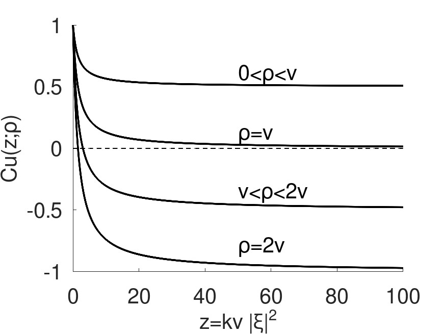
Figure 1: Uzawa method: the convergence constant $C_{u}(z;\rho)$ as a function of $z=k\nu|\xi|^{2}$ with parameter $\rho\in(0,2\nu]$.

The above analysis is summarized in Table 1. The rotational projection iteration method takes the advantages of the other two methods: the fast convergence of standard projection for small viscosity values and the Uzawa method for large viscosity values. Therefore, the rotational projection iteration is comparatively indifferent to viscosity variations.

Table 1: Normal mode analysis when the convection is neglected. The pressure update is $p^{s+1}={p}^{s}-(\rho+\frac{\alpha}{k}(-\Delta)^{-1})(\nabla\cdot{u}^{s})$.

method	pressure iteration	Convergence constant	parameter range	notes
rotational projection	$\alpha=1.5$, $\rho=\nu$	0
standard projection	$\alpha=1.5$, $\rho=0$	$\frac{k\nu|\xi|^{2}}{1.5+k\nu|\xi|^{2}}$		Convergence is fast when $k\nu|\xi|^{2}$ is small
Uzawa	$\alpha=0$	$\frac{1.5+k(\nu-\rho)|\xi|^{2}}{1.5+k\nu|\xi|^{2}}$	$0<\rho\leq 2\nu$	Convergence is fast when $\rho=\nu$ and $k\nu|\xi|^{2}$ is large.

2.2 Iteration analysis with mixed finite element method

If there is no convection or the convection term is treated utterly explicitly, the iteration convergence for a special case when $\rho=\nu$ has been proven in [3], whose proof utilizes the eigenvalue analysis in [8]. Here, we present a self-contained convergence study for the general case with parameters $\alpha$ and $\rho$ in Section 2.2.1. More efforts are spent on the semi-implicit and fully implicit convection cases, as shown in Section 2.2.2 and Section 2.2.3, respectively.

We denote $L^{2}(\Omega)$ as the Lebesgue space of square integrable functions with inner product $(u,v)=\int_{\Omega}u(x)v(x)\mathrm{d}x$, and the $L^{2}$ norm as $\|u\|_{L^{2}(\Omega)}=\sqrt{(u,u)}$. Denote $H^{1}_{0}(\Omega)=\{f:f,\frac{\partial f}{\partial x_{i}}\in L^{2}(\Omega),i=1,2,3,f|_{\partial\Omega}=0\}$. We introduce

$$V =\{u=(u_{1},u_{2},u_{3}):u_{i}\in H^{1}_{0}(\Omega),i=1,2,3\},$$ (27)

$$Q =L^{2}(\Omega)/\mathbb{R}=\{q\in L^{2}(\Omega):\frac{1}{|\Omega|}\int_{\Omega}q(x)\mathrm{d}x=0\},$$ (28)

with the norm $|u|_{1}=(\int_{\Omega}|\nabla u(x)|^{2}\mathrm{d}x)^{1/2}$, where $|\nabla u|^{2}=\sum_{i,j=1}^{3}|\frac{\partial u_{i}}{\partial x_{j}}|^{2}$ and $\frac{1}{|\Omega|}\int_{\Omega}q(x)\mathrm{d}x$ is the average of $q$ over $\Omega$. Let $V_{h}\subset V$ and $Q_{h}\subset Q$ be a pair of conforming mixed finite element spaces approximating the velocity and pressure, respectively, which satisfies the inf-sup condition (a.k.a. the Ladyzhenskaya-Babuka-Brezzi (LBB) condition, see e.g. [13]), i.e.,

$$\inf_{q\in Q_{h}}\sup_{v\in V_{h}}\frac{(\nabla\cdot v,q)}{\|q\|_{L^{2}(\Omega)/\mathbb{R}}|v|_{1}}>0.$$ (29)

Denote the basis of $V_{h}$ as $w_{i},i=1,\cdots,l$, and the basis of $Q_{h}$ as $q_{j},j=1,\cdots,m$.

Definition 1.

A velocity field $u_{h}\in V_{h}$ is weakly divergence free if $(\nabla\cdot u_{h},q_{h})=0$ for all $q_{h}\in Q_{h}$ and strongly divergence free if $\nabla\cdot u_{h}$ is almost everywhere zero in $\Omega$. A pair of mixed finite element spaces $V_{h}$ and $Q_{h}$ is called divergence free if $\nabla\cdot V_{h}\subset Q_{h}$, where $\nabla\cdot V_{h}$ is the range of the divergence of $V_{h}$. Furthermore, a finite element method with a pair of divergence free finite element spaces is called a div-free FEM, and otherwise a non-div-free FEM.

In this work, we use a weak incompressibility measure (267) (a strong incompressiblity measure (269)) to check whether a velocity is weakly (strongly) divergence free. A weakly divergence free velocity may be not pointwise divergence free, as seen in Section 4.2. However, under a pair of divergence free FEM spaces, a weakly divergence free velocity is also strongly divergence free. Indeed, if $u_{h}$ satisfies $(\nabla\cdot u_{h},q_{h})=0$ for all $q_{h}\in Q_{h}$ and $\nabla\cdot V_{h}\subset Q_{h}$, then $\|\nabla\cdot u_{h}\|_{L^{2}(\Omega)}=0$ by choosing $q_{h}=\nabla\cdot u_{h}$, which suggests $\nabla\cdot u_{h}$ is zero almost everywhere in $\Omega$. One popular example of divergence free elements is Scott–Vogelius pair [27]. However, many $H^{1}$-conforming, inf-sup stable mixed finite elements pairs are not divergence free, including the very popular Tayor-Hood elements.

2.2.1 Iteration analysis without convection

Without the convection term, the weak form of the problem (13), (14) and (15) in the mixed finite element method is finding ${u}^{s}\in V_{h}$, $\phi^{s}\in Q_{h}$, $p^{s}\in L^{2}(\Omega)$, such that

$$1.5({u^{s}},{w_{i}})+k\nu(\nabla{u^{s}},\nabla{w_{i}})-k(\nabla\cdot{w_{i}},p^{s})=(F,{w_{i}}), \qquad\forall\,i=1,\cdots,l,$$ (30)

$$(\nabla\phi^{s},\nabla q_{i})=-\frac{1}{k}(\nabla\cdot u^{s},q_{i}), \qquad\forall\,i=1,\cdots,m,$$ (31)

$$(p^{s+1},q_{i})=(p^{s},q_{i})+\alpha(\phi^{s},q_{i})-\rho(\nabla\cdot{u}^{s},q_{i}), \qquad\forall\,i=1,\cdots,m.$$ (32)

The matrices $A_{l\times l}$, $B_{m\times l}$, $G_{m\times m}$, and $M_{m\times m}$ are introduced as follows,

$$A_{ij} =1.5(w_{i},w_{j})+k\nu(\nabla w_{i},\nabla w_{j}),\qquad\forall\,i,j=1,\cdots,l;$$ (33)

$$B_{ij} =-(q_{i},\nabla\cdot w_{j}),\qquad\forall\,i=1,\cdots,m,\ \forall\,j=1,\cdots,l;$$ (34)

$${G}_{ij} =(\nabla q_{i},\nabla q_{j}),\qquad\forall\,i,j=1,\cdots,m;$$ (35)

$$M_{ij} =(q_{j},q_{j}),\qquad\forall\,i,j=1,\cdots,m.$$ (36)

The transpose of $B$ is written as $B^{t}$. Denote the vector $\vec{f}$ as $\vec{f}=((F,w_{1})\cdots(F,w_{l}))^{t}$. We express the following functions as the linear combinations of basis functions, i.e., $u^{s}=\sum_{i=1}^{l}u^{s}_{i}w_{i}$, $\phi^{s}=\sum_{i=1}^{m}\phi^{s}_{i}q_{i}$, $p^{s}=\sum_{i=1}^{m}p^{s}_{i}q_{i}$ and denote the corresponding vector forms as

$$\vec{u}^{s}=\left(\begin{array}[]{c}u^{s}_{1}\\ \vdots\\ u^{s}_{l}\end{array}\right),\quad\vec{\phi}^{s}=\left(\begin{array}[]{c}\phi^{s}_{1}\\ \vdots\\ \phi^{s}_{m}\end{array}\right),\quad\vec{p}^{\,s}=\left(\begin{array}[]{c}p^{s}_{1}\\ \vdots\\ p^{s}_{m}\end{array}\right).$$ (46)

Thereafter, the transformation between the function form and the vector form of a quantity will be used in this way. Thus, the numerical scheme, (30), (31), and (32), is turned into the following matrix-vector form,

$$A\vec{u}^{s}+kB^{t}\vec{p}^{\,s} =\vec{f},$$ (47)

$$G\vec{\phi}^{s} =\frac{1}{k}B\vec{u^{s}},$$ (48)

$$M\vec{p}^{\,s+1} =M\vec{p}^{\,s}+\alpha M\vec{\phi}^{s}+\rho B\vec{u}^{s}.$$ (49)

Without the convection, the weak solution of (4) and (5) is $(u,p)\in V_{h}\times Q_{h}$ satisfying

$$1.5(u,{w_{i}})+k\nu(\nabla u,\nabla{w_{i}})-k(\nabla\cdot{w_{i}},p)=(F,{w_{i}}), \qquad\forall\,i=1,\cdots,l,$$ (50)

$$(\nabla\cdot u,q_{i})=0, \qquad\forall\,i=1,\cdots,m.$$ (51)

The corresponding vector form is

$$A\vec{u}+kB^{t}\vec{p} =\vec{f},$$ (52)

$$G\vec{\phi} =\frac{1}{k}B\vec{u},$$ (53)

$$M\vec{p} =M\vec{p}+\alpha M\vec{\phi}+\rho B\vec{u}.$$ (54)

The last two equations (52) and (53) can be reduced to $\left(G+\frac{\alpha}{k\rho}M\right)\vec{\phi}=0$, whose solution is $\vec{\phi}=0$ since both $G$ and $M$ are symmetric and positive definite. Thus, (53) and (54) are equivalent to

$$B\vec{u}=\vec{0}.$$ (55)

But we keep the current form to compare with (48) and (49).

Denote the errors in the function form as

$${\bar{u}}^{s}={u}^{s}-{u},\qquad{\bar{\phi}}^{s}={\phi}^{s}-{\phi},\qquad{\bar{p}}^{s}={p}^{s}-{p},$$ (56)

and the corresponding errors in the vector form as

$$\vec{\bar{u}}^{s}=\vec{u}^{s}-\vec{u},\qquad\vec{\bar{\phi}}^{s}=\vec{\phi}^{s}-\vec{\phi},\qquad\vec{\bar{p}}^{\,s}=\vec{p}^{\,s}-\vec{p}.$$ (57)

The subtractions of these equations, (47)-(52), (48)-(53), (49)-(54), give rise to

$$A\vec{\bar{u}}^{s}+kB^{t}\vec{\bar{p}}^{\,s} =0,$$ (58)

$$G\vec{\bar{\phi}}^{s} =\frac{1}{k}B\vec{\bar{u}}^{s},$$ (59)

$$\vec{\bar{p}}^{\,s+1} =\vec{\bar{p}}^{\,s}+\alpha\vec{\bar{\phi}}^{s}+\rho M^{-1}B\vec{\bar{u}}^{s}.$$ (60)

From (58) and (59) we get

$$\vec{\bar{u}}^{s} =-kA^{-1}B^{t}\vec{\bar{p}}^{\,s},$$ (61)

$$\vec{\bar{\phi}}^{s} =-G^{-1}BA^{-1}B^{t}\vec{\bar{p}}^{\,s}.$$ (62)

Let

$$D=BA^{-1}B^{t},$$ (63)

which is the negative Schur complement of $A$ (e.g., see [5]), then

$$\vec{\bar{p}}^{\,s+1}=(I-(\alpha G^{-1}+\rho kM^{-1})D)\vec{\bar{p}}^{\,s}\triangleq(I-K)\vec{\bar{p}}^{\,s},$$ (64)

where

$$K_{m\times m}=(\alpha G^{-1}+\rho kM^{-1})D.$$ (65)

To study the convergence, we will analyze the eigenvalues of the matrix $K$. First, we introduce the following lemmas.

Lemma 1.

Let $S$, $T$ be symmetric matrices. If $S$ is positive definite, then $S^{-1}T$ is diagonalizable.

Proof.
Since $S$ is symmetric and positive definite (SPD), its inverse $S^{-1}$ is also SPD. Denote its square root as $S^{-1/2}$. Then $S^{1/2}S^{-1}TS^{-1/2}=S^{-1/2}TS^{-1/2}$, where the latter is symmetric because $T$ and $S^{-1/2}$ are both symmetric. Therefore, $S^{-1}T$ is similar to a symmetric matrix and hence diagonalizable.

$\Box$

Lemma 2.

All the eigenvalues of $K$ are positive and $K$ has a set of linearly independent eigenvectors that span $\mathbb{R}^{m}$, which is called an eigenbasis of $K$.

Proof.
First, note that without the convection term the matrix $A$ is SPD. The inf-sup condition guarantees $B$ has the full row rank and then the matrix $D$ is also SPD. In addition, the matrices $G$ and $M$ are also SPD.

Suppose $\lambda$ is an eigenvalue of $K$ and $\vec{\xi}\in\mathbb{R}^{m}$ is an associated eigenvector, i.e., $K\vec{\xi}=\lambda\vec{\xi}$. Left-multiplying both sides by $\vec{\xi}^{\,t}D$ leads to

$$\alpha\vec{\xi}^{\,t}DG^{-1}D\vec{\xi}+\rho k\vec{\xi}^{\,t}DM^{-1}D\vec{\xi}=\lambda\vec{\xi}^{\,t}D\vec{\xi}.$$ (66)

Since the quantities $\alpha$, $\rho$, $k$, $\vec{\xi}^{\,t}DG^{-1}D\vec{\xi}$, $\vec{\xi}^{\,t}DM^{-1}D\vec{\xi}$, $\vec{\xi}^{\,t}D\vec{\xi}$ are all positive, the value of $\lambda$ must be positive.

Furthermore, a matrix is diagonalizable if and only if there is a set of eigenbasis of this matrix (e.g., [20] Theorem 1.3.7, p. 59). In the matrix $K$, the left factor $(\alpha G^{-1}+\rho kM^{-1})$ is SPD and the right factor $D$ is symmetric. According to Lemma 1, $K$ has an eigenbasis.

$\Box$

Denote an eigenbasis of $K$ as $\{\vec{\xi}_{1},\cdots,\vec{\xi}_{m}\}$ and the corresponding eigenvalues as $\lambda_{j},j=1,\cdots,m$. Let $\rho(I-K)$ be the spetral radius of $I-K$, that is,

$$\rho(I-K)=\max_{j=1,\cdots,m}|1-\lambda_{j}|.$$ (67)

Because all eigenvalues are positive according to Lemma 2, it is easy to deduce from (67) that

Lemma 3.

$\rho(I-K)<1$ if and only if $\lambda_{\max}<2$.

The next lemma gives an upper bound of the largest eigenvalue $K$ dependent on the parameters in the numerical scheme.

Lemma 4.

Let $\lambda_{\max}$ be the largest eigenvalue of $K$, then

$$\lambda_{\max}\leq\max\left(\frac{\alpha}{1.5},\frac{\rho}{\nu}\right).$$ (68)

Proof.
Let $\lambda$ be an eigenvalue of $K$ and $\vec{\xi}$ be an associated eigenvector. According to (66),

$$\lambda=\frac{\alpha\langle G^{-1}D\vec{\xi},D\vec{\xi}\rangle+\rho k\langle M^{-1}D\vec{\xi},D\vec{\xi}\rangle}{\langle D\vec{\xi},\vec{\xi}\rangle},$$ (69)

where the notation $\langle\vec{\xi},\vec{q}\rangle\triangleq\vec{\xi}^{\,t}\vec{q}$ for any two vectors in the same Euclidean space $\mathbb{R}^{m}$ or $\mathbb{R}^{l}$. Denote $\vec{v}=A^{-1}B^{t}\vec{\xi}$, i.e., $A\vec{v}=B^{t}\vec{\xi}$ or $D\vec{\xi}=B\vec{v}$. Then (69) becomes

$$\lambda=\frac{\alpha\langle G^{-1}B\vec{v},B\vec{v}\rangle+\rho k\langle M^{-1}B\vec{v},B\vec{v}\rangle}{\langle\vec{v},A\vec{v}\rangle}=\frac{\alpha\langle G^{-1}B\vec{v},B\vec{v}\rangle+\rho k\langle M^{-1}B\vec{v},B\vec{v}\rangle}{1.5\|v\|^{2}_{L^{2}(\Omega)}+\nu k\|\nabla v\|^{2}_{L^{2}(\Omega)}}\triangleq R(\vec{v}).$$ (70)

This equates the eigenvalues to the stationary values of the Rayleigh quotient $R(\vec{v})$ defined in (70). To estimate the two numerator terms in (70), let $\vec{\phi}=G^{-1}B\vec{v}$, then $G\vec{\phi}=B\vec{v}$. Using the connection between the vector and function forms: $\vec{\phi}=(\phi_{1}\cdots\phi_{m})^{t}$ and $\phi=\sum_{i=1}^{m}\phi_{i}q_{i}$, $\vec{v}=(v_{1}\cdots v_{l})^{t}$ and $v=\sum_{i=1}^{l}v_{i}w_{i}$, we see that $G\vec{\phi}=B\vec{v}$ is equivalent to

$$\int_{\Omega}\nabla\phi\cdot\nabla\eta\mathrm{d}x=-\int_{\Omega}(\nabla\cdot v)\eta\mathrm{d}x,\quad\forall\eta\in Q_{h}.$$ (71)

Afterwards,

$$\langle G^{-1}B\vec{v},B\vec{v}\rangle=\langle\vec{\phi},B\vec{v}\rangle=-\int_{\Omega}\phi(\nabla\cdot v)\mathrm{d}x.$$ (72)

Using $\eta=\phi$ in (71), integration by parts, and Young’s inequality, we get

$$\|\nabla\phi\|_{L^{2}(\Omega)}^{2}=-\int_{\Omega}\phi(\nabla\cdot v)\mathrm{d}x=\int_{\Omega}v\cdot\nabla\phi\mathrm{d}x\leq\frac{1}{2}\big{(}\|v\|^{2}_{L^{2}(\Omega)}+\|\nabla\phi\|^{2}_{L^{2}(\Omega)}\big{)},$$ (73)

which further gives $\|\nabla\phi\|_{L^{2}(\Omega)}^{2}\leq\|v\|^{2}_{L^{2}(\Omega)}$. Thus,

$$\langle G^{-1}B\vec{v},B\vec{v}\rangle=\|\nabla\phi\|^{2}_{L^{2}(\Omega)}\leq\|v\|^{2}_{L^{2}(\Omega)}.$$ (74)

To study $\langle M^{-1}B\vec{v},B\vec{v}\rangle$, we let $\vec{y}=M^{-1}B\vec{v}$, i.e., $M\vec{y}=B\vec{v}$. Suppose the vector $\vec{y}=(y_{1}\cdots y_{m})^{t}$ and the corresponding function $y=\sum_{i=1}^{m}y_{i}q_{i}$. Then $M\vec{y}=B\vec{v}$ can be rewritten as

$$\int_{\Omega}y\eta\mathrm{d}x=-\int_{\Omega}(\nabla\cdot v)\eta\mathrm{d}x,\quad\forall\eta\in Q_{h}.$$ (75)

Letting $\eta=y$, then

$$\|y\|^{2}_{L^{2}(\Omega)}=-\int_{\Omega}(\nabla\cdot v)y\mathrm{d}x\leq\frac{1}{2}\big{(}\|\nabla\cdot v\|^{2}_{L^{2}(\Omega)}+\|y\|^{2}_{L^{2}(\Omega)}\big{)}.$$ (76)

This results in $\|y\|_{L^{2}(\Omega)}\leq\|\nabla\cdot v\|_{L^{2}(\Omega)}$. It is also known that for any $v\in[H_{0}^{1}(\Omega)]^{3}$, for example, [29] p. 93,

$$\|\nabla\cdot v\|_{L^{2}(\Omega)}\leq\|\nabla v\|_{L^{2}(\Omega)}.$$ (77)

Afterwards,

$$\langle M^{-1}B\vec{v},B\vec{v}\rangle=\langle\vec{y},B\vec{v}\rangle=-\int_{\Omega}(\nabla\cdot v)y\mathrm{d}x=\|y\|^{2}_{L^{2}(\Omega)}\leq\|\nabla\cdot v\|_{L^{2}(\Omega)}^{2}\leq\|\nabla v\|_{L^{2}(\Omega)}^{2}.$$ (78)

Collecting (70), (74), (78), we obtain

$$\lambda_{\max}\leq\frac{\alpha\|v\|^{2}_{L^{2}(\Omega)}+\rho k\|\nabla v\|^{2}_{L^{2}(\Omega)}}{1.5\|v\|^{2}_{L^{2}(\Omega)}+\nu k\|\nabla v\|^{2}_{L^{2}(\Omega)}}\leq\max\left(\frac{\alpha}{1.5},\frac{\rho}{\nu}\right).$$ (79)

$\Box$

We introduce the maximum vector norm with respect to the eigenbasis $\{\vec{\xi}_{i}\}_{i=1}^{m}$ of $K$, that is,

$$\|\vec{q}\|_{K,\infty}=\max_{1\leq j\leq m}|q_{K,j}|\text{ when }\vec{q}=\sum_{j=1}^{m}q_{K,j}\vec{\xi}_{j}.$$ (80)

Theorem 1 (Iteration convergence without convection).

The pressure solution error $\vec{\bar{p}}^{\,s}$ between the scheme (47), (48), (49) and the system (52), (53), (54) satisfies

$$\|\vec{\bar{p}}^{\,s+1}\|_{K,\infty}\leq\rho(I-K)\|\vec{\bar{p}}^{\,s}\|_{K,\infty}.$$ (81)

Thus, if $\rho(I-K)<1$, then the iterative solution (${u}^{s}$, ${p}^{\,s}$) of (30), (31), (32) converges linearly to (${u}$, ${p}$) of (50), (51). In particular, if $\max\left(\frac{\alpha}{1.5},\frac{\rho}{\nu}\right)<2$, then $\rho(I-K)<1$. Furthermore, the convergence of iteration is independent of the time step size $k$.

Proof.
Express the error $\vec{\bar{p}}^{\,s}=\sum_{j=1}^{m}\bar{p}^{s}_{K,j}\vec{\xi}_{j}$. Then (64) becomes

$$\sum_{j=1}^{m}\bar{p}^{s+1}_{K,j}\vec{\xi}_{j}=\sum_{j=1}^{m}(1-\lambda_{j})\bar{p}^{s}_{K,j}\vec{\xi}_{j}.$$ (82)

Due to the linear independency of $\{\vec{\xi}_{j}\}_{j=1}^{m}$, we arrive at

$$\bar{p}^{s+1}_{K,j}=(1-\lambda_{j})\bar{p}^{s}_{K,j},\quad j=1,\cdots,m.$$ (83)

Taking maximum values on both sides yields (81). By Lemma 3 and Lemma 4, if $\max\left(\frac{\alpha}{1.5},\frac{\rho}{\nu}\right)<2$, then $\rho(I-K)<1$.

$\Box$

2.2.2 Iteration analysis with semi-implicit convection

When the semi-implicit convection form $\text{NL}(w,u)$ is used, the weak form of the saddle point problem (4) and (5) is composed by (51) and

$$1.5({u},{w_{i}})+k\nu(\nabla u,\nabla{w_{i}})+k(\text{NL}(w,u),w_{i})-k(\nabla\cdot{w_{i}},p)=(F,{w_{i}}),\quad\forall\,i=1,\cdots,l.$$ (84)

Accordingly, the weak form of (13) turns to

$$1.5({u^{s}},{w_{i}})+k\nu(\nabla{u^{s}},\nabla{w_{i}})+k(\text{NL}(w,u^{s}),w_{i})-k(\nabla\cdot{w_{i}},p^{s})=(F,{w_{i}}),\quad\forall\,i=1,\cdots,l.$$ (85)

The entire semi-implicit iterative projection scheme includes (85), (31), (32). Define the matrices $N(w)$ and $A_{N}(w)$ as, respectively,

$$N(w)_{ij} =(\text{NL}(w,w_{j}),w_{i}),\quad\forall\,i,j=1,\cdots,l,$$ (86)

$$A_{N}(w) =A+kN(w).$$ (87)

Then (84) and (85) can be written as

$$A_{N}(w)\vec{u}+kB^{t}\vec{p} =\vec{f},$$ (88)

$$A_{N}(w)\vec{u}^{s}+kB^{t}\vec{p}^{\,s} =\vec{f}.$$ (89)

The proofs of iteration convergence with both SI and FI convection forms are by writing the system as a perturbation with the coefficient $k$ of the non-convection system, (64). This is done for SI schemes in (100), (103), and for FI schemes in (141). The perturbation terms with the coefficient $k$ depend on the convection matrix $N(w)$, which has an upper bound given in Lemma 5. Then, a sufficiently small $k$ keeps the system as a contraction. To earn this upper bound, we adopt the spectral matrix norm ${\left|\kern-1.07639pt\left|\kern-1.07639pt\left|\cdot\right|\kern-1.07639pt\right|\kern-1.07639pt\right|}_{2}$ for square matrices, which is induced by the Euclidean metric in $\mathbb{R}^{l}$. For more details of this norm, see, e.g., [20, Section 5.6]. As for the spectral norm of $N(w)$, the following upper bound on $\|w\|_{L^{2}(\Omega)}$ when $w\in V_{h}$ is provided.

Lemma 5.

There exists a constant $C$ only dependent on $h$ and the basis of $V_{h}$ such that

$$|(\text{NL}(u,v),w)| \leq C\|u\|_{L^{2}(\Omega)}\|v\|_{L^{2}(\Omega)}\|w\|_{L^{2}(\Omega)},\quad\forall u,v,w\in V_{h},$$ (90)

$${\left|\kern-1.07639pt\left|\kern-1.07639pt\left|N(w)\right|\kern-1.07639pt\right|\kern-1.07639pt\right|}_{2} \leq C\|w\|_{L^{2}(\Omega)},\quad\forall w\in V_{h}.$$ (91)

Proof.
Using [20, Theorem 5.4.17 and 5.6.2(d)], ${\left|\kern-1.07639pt\left|\kern-1.07639pt\left|N(w)\right|\kern-1.07639pt\right|\kern-1.07639pt\right|}_{2}=\max_{\|\vec{\xi}\|_{2}=\|\vec{\eta}\|_{2}=1}{\vec{\xi}}^{t}N(w)\vec{\eta}$, where $\vec{\xi},\vec{\eta}\in\mathbb{R}^{l}$. Using the connection between the vector and function forms: $\vec{\xi}=(\xi_{1}\cdots\xi_{l})^{t}$, $\xi=\sum_{i=1}^{l}\xi_{i}w_{i}$, $\vec{\eta}=(\eta_{1}\cdots\eta_{l})^{t}$, $\eta=\sum_{i=1}^{l}\eta_{i}w_{i}$, we obtain $\vec{\xi}^{t}N(w)\vec{\eta}=\sum_{i,j=1}^{l}\xi_{i}((w\cdot\nabla)w_{i},w_{i})\eta_{j}=((w\cdot\nabla)\xi,\eta)$. Hence,

$${\left|\kern-1.07639pt\left|\kern-1.07639pt\left|N(w)\right|\kern-1.07639pt\right|\kern-1.07639pt\right|}_{2}=\max_{\|\vec{\xi}\|_{2}=\|\vec{\eta}\|_{2}=1}((w\cdot\nabla)\xi,\eta).$$ (92)

Note that

$$|((w\cdot\nabla)\xi,\eta)| =\bigg{|}\int_{\Omega}((w\cdot\nabla)\xi)\cdot\eta\mathrm{d}x\bigg{|},$$ (93)

$$\leq\|w\|_{L^{4}(\Omega)}\|\eta\|_{L^{4}(\Omega)}\|\nabla\xi\|_{L^{2}(\Omega)}$$ (94)

$$\leq 2\|w\|^{\frac{1}{4}}_{L^{2}(\Omega)}\|\nabla w\|^{\frac{3}{4}}_{L^{2}(\Omega)}\|\eta\|^{\frac{1}{4}}_{L^{2}(\Omega)}\|\nabla\eta\|^{\frac{3}{4}}_{L^{2}(\Omega)}\|\nabla\xi\|_{L^{2}(\Omega)},$$ (95)

where (94) is obtained by Hölder’s inequality and (95) by Ladyzhenskaya’s inequality in three-dimensional case, $\|v\|_{L^{4}(\Omega)}\leq\sqrt{2}\|v\|^{1/4}_{L^{2}(\Omega)}\|\nabla v\|^{3/4}_{L^{2}(\Omega)}$, $\forall v\in V$ (see, e.g., [29, Lemma 3.5, p. 200]). Next, by applying the inverse inequality $\|\nabla v\|_{L^{2}(\Omega)}\leq Ch^{-1}\|v\|_{L^{2}(\Omega)}$ for any $v\in V_{h}$ (e.g., [6, Theorem 4.5.11, p. 112]), where $C$ only depends on $\Omega$, the above estimates continue as

$$|((w\cdot\nabla)\xi,\eta)| \leq 2\|w\|^{\frac{1}{4}}_{L^{2}(\Omega)}(Ch^{-1})^{\frac{3}{4}}\|w\|^{\frac{3}{4}}_{L^{2}(\Omega)}\|\eta\|^{\frac{1}{4}}_{L^{2}(\Omega)}(Ch^{-1})^{\frac{3}{4}}\|\eta\|^{\frac{3}{4}}_{L^{2}(\Omega)}Ch^{-1}\|\xi\|_{L^{2}(\Omega)}$$ (96)

$$\leq Ch^{-\frac{5}{2}}\|w\|_{L^{2}(\Omega)}\|\xi\|_{L^{2}(\Omega)}\|\eta\|_{L^{2}(\Omega)}$$ (97)

$$=C\|w\|_{L^{2}(\Omega)}\|\xi\|_{L^{2}(\Omega)}\|\eta\|_{L^{2}(\Omega)},$$ (98)

where the last $C$ absorbs $h^{-2.5}$ in the previous step. Note the inequality (98) holds for any $\xi,\eta\in V_{h}$, which leads to (90).

But $\|\xi\|^{2}_{L^{2}(\Omega)}=(\sum_{i=1}^{l}\xi_{i}w_{i},\sum_{j=1}^{l}\xi_{j}w_{j})=\sum_{i,j=1}^{l}\xi_{i}\xi_{j}(w_{i},w_{j})=\vec{\xi}^{t}A_{0}\vec{\xi}$, where $A_{0}$ is the mass matrix of $V_{h}$ with $(A_{0})_{ij}=(w_{i},w_{j})$. Clearly, $A_{0}$ is symmetric and positive definite. Since $\|\vec{\xi}\|_{2}=1$, $\vec{\xi}^{t}A_{0}\vec{\xi}\leq\rho(A_{0})$, the spectral radius of $A_{0}$. Thus, $\|\xi\|_{L^{2}(\Omega)}\leq\sqrt{\rho(A_{0})}$ and similarly $\|\eta\|_{L^{2}(\Omega)}\leq\sqrt{\rho(A_{0})}$. Therefore,

$$|((w\cdot\nabla)\xi,\eta)|\leq C\rho(A_{0})\|w\|_{L^{2}(\Omega)}\leq C\|w\|_{L^{2}(\Omega)},$$ (99)

where $C\rho(A_{0})$ is denoted as a new $C$ in the final step, which only depends on $h$ and the basis of $V_{h}$. Finally, (91) is achieved from (92) and (99).

$\Box$

Lemma 6.

If the time step size $k$ is sufficiently small, then the symmetric part of $A_{N}(w)$, $H\triangleq\frac{1}{2}(A_{N}(w)+A_{N}^{t}(w))$, is positive definite.

Remark 1.

This implies the system of (88) and (55) is a generalized saddle point problem according to [5].

Proof.
Let $\vec{v}=(v_{1}\cdots v_{l})^{t}\in\mathbb{R}^{l}$ and $v=\sum_{i=1}^{l}v_{i}w_{i}$, then

$$\vec{v}^{t}H\vec{v} =\vec{v}^{t}A\vec{v}+\frac{k}{2}\vec{v}^{t}(N(w)+N^{t}(w))\vec{v}$$

$$=\|v\|^{2}_{L^{2}(\Omega)}+k\|\nabla v\|^{2}_{L^{2}(\Omega)}+\frac{k}{2}((\text{NL}(w),v),v)+\text{NL}(v,w),w))$$

$$\geq\|v\|^{2}_{L^{2}(\Omega)}-kC\|w\|_{L^{2}(\Omega)}\|v\|^{2}_{L^{2}(\Omega)}=(1-kC\|w\|_{L^{2}(\Omega)})\|v\|^{2}_{L^{2}(\Omega)},$$

where $(\text{NL}(w),v),v),(\text{NL}(v),w),v)\geq-C\|w\|_{L^{2}(\Omega)}\|v\|^{2}_{L^{2}(\Omega)}$ from Lemma 5 is used in the last step. If $k<1/(C\|w\|_{L^{2}(\Omega)})$, then $H$ is positive definite.

$\Box$

Using the same process of obtaining (64) in the case without convection, we obtain that the pressure solution error between the scheme (89), (48), (49) and the system (88), (53), (54) satisfies

$$\vec{\bar{p}}^{\,s+1}=(I-K_{N}(w))\vec{\bar{p}}^{\,s},$$ (100)

where

$$K_{N}(w)\triangleq(\alpha G^{-1}+\rho kM^{-1})BA^{-1}_{N}(w)B^{t}.$$ (101)

The equation (85) can be regarded as a first order perturbation in time step size $k$ of (30). The following lemma indicates that $I-K_{N}(w)$ is also a first order perturbation of $I-K$.

Lemma 7.

For each $w\in V_{h}$, there exists $k_{w}>0$, such that when $0<k<\min(k_{w},1)$, the matrix $A_{N}(w)$ is invertible,

$${\left|\kern-1.07639pt\left|\kern-1.07639pt\left|A^{-1}_{N}(w)\right|\kern-1.07639pt\right|\kern-1.07639pt\right|}_{2}\leq C(1+k\|w\|_{L^{2}(\Omega)}),$$ (102)

and

$$I-K_{N}(w)=I-K-kA_{N2}(w),$$ (103)

where

$${\left|\kern-1.07639pt\left|\kern-1.07639pt\left|A_{N2}(w)\right|\kern-1.07639pt\right|\kern-1.07639pt\right|}_{2}\leq C\|w\|_{L^{2}(\Omega)}.$$ (104)

Here, the constants $C$ are independent of $w$, but depend on $h$ and bases of $V_{h}$ and $Q_{h}$.

Proof.
Note $A_{N}(w)=A+kN(w)=A(I+kA^{-1}N(w))$. When $w$ and the basis of $V_{h}$ are fixed, the matrices $A$ and $N(w)$ are also fixed. Note $A_{N}$ is invertible if and only if $(I+kA^{-1}N(w))$ is invertible. According to [20, Corollary 5.6.16], $(I+kA^{-1}N(w))$ being invertible is equivalent to $k{\left|\kern-1.07639pt\left|\kern-1.07639pt\left|A^{-1}N(w)\right|\kern-1.07639pt\right|\kern-1.07639pt\right|}_{2}<1$.

Let

$$k_{w}=\frac{0.5}{C{\left|\kern-1.07639pt\left|\kern-1.07639pt\left|A^{-1}\right|\kern-1.07639pt\right|\kern-1.07639pt\right|}_{2}\|w\|_{L^{2}(\Omega)}},$$ (105)

where the value of $C$ is the one in (91). If $0<k<k_{w}$, then $k{\left|\kern-1.07639pt\left|\kern-1.07639pt\left|A^{-1}N(w)\right|\kern-1.07639pt\right|\kern-1.07639pt\right|}_{2}\leq k{\left|\kern-1.07639pt\left|\kern-1.07639pt\left|A^{-1}\right|\kern-1.07639pt\right|\kern-1.07639pt\right|}_{2}{\left|\kern-1.07639pt\left|\kern-1.07639pt\left|N(w)\right|\kern-1.07639pt\right|\kern-1.07639pt\right|}_{2}\leq kC{\left|\kern-1.07639pt\left|\kern-1.07639pt\left|A^{-1}\right|\kern-1.07639pt\right|\kern-1.07639pt\right|}_{2}\|w\|_{L^{2}(\Omega)}<0.5$. Thus, the matrix $(I+kA^{-1}N(w))$ is invertible and $(I+kA^{-1}N(w))^{-1}=I+kA_{N1}(w)$, where

$$A_{N1}(w)\triangleq\sum_{j=1}^{\infty}(-1)^{j}k^{j-1}(A^{-1}N(w))^{j}$$ (106)

and

$${\left|\kern-1.07639pt\left|\kern-1.07639pt\left|A_{N1}(w)\right|\kern-1.07639pt\right|\kern-1.07639pt\right|}_{2}\leq\frac{{\left|\kern-1.07639pt\left|\kern-1.07639pt\left|A^{-1}N(w)\right|\kern-1.07639pt\right|\kern-1.07639pt\right|}_{2}}{1-k{\left|\kern-1.07639pt\left|\kern-1.07639pt\left|A^{-1}N(w)\right|\kern-1.07639pt\right|\kern-1.07639pt\right|}_{2}}\leq 2{\left|\kern-1.07639pt\left|\kern-1.07639pt\left|A^{-1}\right|\kern-1.07639pt\right|\kern-1.07639pt\right|}_{2}{\left|\kern-1.07639pt\left|\kern-1.07639pt\left|N(w)\right|\kern-1.07639pt\right|\kern-1.07639pt\right|}_{2}.$$ (107)

Thus, when $0<k<k_{w}$, $A_{N}(w)$ is invertible and

$$A^{-1}_{N}(w)=(I+kA_{N1}(w))A^{-1}=A^{-1}+kA_{N1}(w)A^{-1}.$$ (108)

Furthermore,

$${\left|\kern-1.07639pt\left|\kern-1.07639pt\left|A^{-1}_{N}(w)\right|\kern-1.07639pt\right|\kern-1.07639pt\right|}_{2} ={\left|\kern-1.07639pt\left|\kern-1.07639pt\left|(I+kA_{N1}(w))A^{-1}\right|\kern-1.07639pt\right|\kern-1.07639pt\right|}_{2}\leq{\left|\kern-1.07639pt\left|\kern-1.07639pt\left|A^{-1}\right|\kern-1.07639pt\right|\kern-1.07639pt\right|}_{2}(1+k{\left|\kern-1.07639pt\left|\kern-1.07639pt\left|A_{N1}(w)\right|\kern-1.07639pt\right|\kern-1.07639pt\right|}_{2})$$ (109)

$$\leq{\left|\kern-1.07639pt\left|\kern-1.07639pt\left|A^{-1}\right|\kern-1.07639pt\right|\kern-1.07639pt\right|}_{2}(1+2k{\left|\kern-1.07639pt\left|\kern-1.07639pt\left|A^{-1}\right|\kern-1.07639pt\right|\kern-1.07639pt\right|}_{2}{\left|\kern-1.07639pt\left|\kern-1.07639pt\left|N(w)\right|\kern-1.07639pt\right|\kern-1.07639pt\right|}_{2})$$ (110)

$$\leq{\left|\kern-1.07639pt\left|\kern-1.07639pt\left|A^{-1}\right|\kern-1.07639pt\right|\kern-1.07639pt\right|}_{2}(1+2Ck{\left|\kern-1.07639pt\left|\kern-1.07639pt\left|A^{-1}\right|\kern-1.07639pt\right|\kern-1.07639pt\right|}_{2}\|w\|_{L^{2}(\Omega)})$$ (111)

$$\leq C^{\prime}(1+k\|w\|_{L^{2}(\Omega)}),$$ (112)

where (107) is used in (109) to get (110), and (91) is applied in (110) to get (111). The $C^{\prime}$ in (112) is $C^{\prime}=\max({\left|\kern-1.07639pt\left|\kern-1.07639pt\left|A^{-1}\right|\kern-1.07639pt\right|\kern-1.07639pt\right|}_{2},2C{\left|\kern-1.07639pt\left|\kern-1.07639pt\left|A^{-1}\right|\kern-1.07639pt\right|\kern-1.07639pt\right|}^{2}_{2})$ from (111). Changing $C^{\prime}$ to a new $C$ results in (102).

Then (101) and (108) lead to

$$I-K_{N}(w) =I-(\alpha G^{-1}+\rho kM^{-1})BA^{-1}B^{t}-k(\alpha G^{-1}+\rho kM^{-1})BA_{N1}(w)A^{-1}B^{t}$$ (113)

$$\triangleq I-K-kA_{N2}(w),$$ (114)

where $K$ is defined in (65) and

$$A_{N2}(w)\triangleq(\alpha G^{-1}+\rho kM^{-1})BA_{N1}(w)A^{-1}B^{t}.$$ (115)

Then

$${\left|\kern-1.07639pt\left|\kern-1.07639pt\left|A_{N2}(w)\right|\kern-1.07639pt\right|\kern-1.07639pt\right|}_{2} \leq(\alpha{\left|\kern-1.07639pt\left|\kern-1.07639pt\left|G^{-1}\right|\kern-1.07639pt\right|\kern-1.07639pt\right|}_{2}+\rho k{\left|\kern-1.07639pt\left|\kern-1.07639pt\left|M^{-1}\right|\kern-1.07639pt\right|\kern-1.07639pt\right|}_{2}){\left|\kern-1.07639pt\left|\kern-1.07639pt\left|B\right|\kern-1.07639pt\right|\kern-1.07639pt\right|}_{2}{\left|\kern-1.07639pt\left|\kern-1.07639pt\left|B^{t}\right|\kern-1.07639pt\right|\kern-1.07639pt\right|}_{2}{\left|\kern-1.07639pt\left|\kern-1.07639pt\left|A^{-1}\right|\kern-1.07639pt\right|\kern-1.07639pt\right|}_{2}{\left|\kern-1.07639pt\left|\kern-1.07639pt\left|A_{N1}(w)\right|\kern-1.07639pt\right|\kern-1.07639pt\right|}_{2}$$ (116)

$$\leq(\alpha{\left|\kern-1.07639pt\left|\kern-1.07639pt\left|G^{-1}\right|\kern-1.07639pt\right|\kern-1.07639pt\right|}_{2}+\rho{\left|\kern-1.07639pt\left|\kern-1.07639pt\left|M^{-1}\right|\kern-1.07639pt\right|\kern-1.07639pt\right|}_{2}){\left|\kern-1.07639pt\left|\kern-1.07639pt\left|B\right|\kern-1.07639pt\right|\kern-1.07639pt\right|}_{2}{\left|\kern-1.07639pt\left|\kern-1.07639pt\left|B^{t}\right|\kern-1.07639pt\right|\kern-1.07639pt\right|}_{2}\cdot 2{\left|\kern-1.07639pt\left|\kern-1.07639pt\left|A^{-1}\right|\kern-1.07639pt\right|\kern-1.07639pt\right|}^{2}_{2}{\left|\kern-1.07639pt\left|\kern-1.07639pt\left|N(w)\right|\kern-1.07639pt\right|\kern-1.07639pt\right|}_{2}$$ (117)

$$=C_{1}{\left|\kern-1.07639pt\left|\kern-1.07639pt\left|N(w)\right|\kern-1.07639pt\right|\kern-1.07639pt\right|}_{2}\leq C\|w\|_{L^{2}(\Omega)},$$ (118)

where we have used $0<k<1$ and (107) to get (117) and Lemma 5 to obtain (118). The constant $C_{1}$ in (118) denotes the product of all terms in front of ${\left|\kern-1.07639pt\left|\kern-1.07639pt\left|N(w)\right|\kern-1.07639pt\right|\kern-1.07639pt\right|}_{2}$ in (117), which only depends on the bases of $V_{h}$ and $Q_{h}$. The identity (114) and estimate (118) conclude this lemma.

$\Box$

The next result presents the recursive relation of the pressure error and the iteration convergence conditions.

Theorem 2 (Iteration Convergence with SI-Iterative Projection Method).

If $k$ is sufficiently small, then the pressure error between (89), (48), (49) and the system (88), (53), (54), where $w$ is explicit, satisfies

$$\|\vec{\bar{p}}^{\,s+1}\|_{K,\infty}\leq\big{(}\rho(I-K)+kC\|w\|_{L^{2}(\Omega)}\big{)}\cdot\|\vec{\bar{p}}^{\,s}\|_{K,\infty},$$ (119)

where $C$ is a constant that only depends on $h$ and the bases of $V_{h}$ and $Q_{h}$. If $\rho(I-K)<1$, which can be guaranteed by enforcing $\max\left(\frac{\alpha}{1.5},\frac{\rho}{\nu}\right)<2$, and $k$ is such that $\rho(I-K)+kC\|w\|_{L^{2}(\Omega)}<1$, then the iteration converges. In this case, the solution $(u^{s},p^{s})$ of (85), (31), (32) converges linearly to $(u,p)$ of (84), (51).

Proof.
According to (100) and Lemma 7,

$$\vec{\bar{p}}^{\,s+1}=(I-K)\vec{\bar{p}}^{\,s}-kA_{N2}(w)\vec{\bar{p}}^{\,s}.$$ (120)

We express $A_{N2}(w)\vec{\bar{p}}^{\,s}$ as a linear combination of the eigenbasis $\{\vec{\xi}_{j}\}_{j=1}^{m}$, i.e.,

$$A_{N2}(w)\vec{\bar{p}}^{\,s}=\sum_{j=1}^{m}\eta_{K,j}\vec{\xi}_{j}=\vec{\eta},$$ (121)

for some real numbers $\eta_{K,j}\in\mathbb{R}$, $j=1,\cdots,m$. Then there exists a constant $C$ merely dependent on the bases of $V_{h}$ and $Q_{h}$ such that

$$\|\vec{\eta}\|_{K,\infty} =\max_{1\leq j\leq m}|\eta_{K,j}|\leq C\|A_{N2}(w)\vec{\bar{p}}^{\,s}\|_{2}\leq C{\left|\kern-1.07639pt\left|\kern-1.07639pt\left|A_{N2}(w)\right|\kern-1.07639pt\right|\kern-1.07639pt\right|}_{2}\|\vec{\bar{p}}^{\,s}\|_{2}$$ (122)

$$\leq C\|w\|_{L^{2}(\Omega)}\|\vec{\bar{p}}^{\,s}\|_{K,\infty},$$ (123)

where (104) is used in the last step and the equivalence of norms in $\mathbb{R}^{m}$ is repeatedly used.

Using the expressions $\vec{\bar{p}}^{\,s+1}=\sum_{j=1}^{m}\bar{p}^{s+1}_{K,j}\vec{\xi}_{j}$ and $\vec{\bar{p}}^{\,s}=\sum_{j=1}^{m}\bar{p}^{s}_{K,j}\vec{\xi}_{j}$, (120) and (121) yield $\sum_{j=1}^{m}\bar{p}^{s+1}_{K,j}\vec{\xi}_{j}=\sum_{j=1}^{m}((1-\lambda_{j})\bar{p}^{s}_{K,j}-k\eta_{K,j})\vec{\xi}_{j}$. The linear independency of the eigenbasis $\{\vec{\xi}\}_{j=1}^{m}$ implies

$$\bar{p}^{s+1}_{K,j}=(1-\lambda_{j})\bar{p}^{s}_{K,j}-k\eta_{K,j},\quad j=1,\cdots,m.$$ (124)

This suggests

$$\|\vec{\bar{p}}^{\,s+1}\|_{K,\infty} \leq \max_{1\leq j\leq m}|1-\lambda_{j}|\cdot\|\vec{\bar{p}}^{\,s}\|_{K,\infty}+k\|\vec{\bar{\eta}}\|_{K,\infty}$$ (125)

$$\leq \rho(I-K)\|\vec{\bar{p}}^{\,s}\|_{K,\infty}+kC\|w\|_{L^{2}(\Omega)}\|\vec{\bar{p}}^{\,s}\|_{K,\infty},$$

where (123) is used in the last step.

When $\max\left(\frac{\alpha}{1.5},\frac{\rho}{\nu}\right)<2$, Lemma 3 and Lemma 4 imply $\rho(I-K)<1$. In the recursive relation (119), if $k$ is sufficiently small, the iteration ratio satisfies $0<\rho(I-K)+kC\|w\|_{L^{2}(\Omega)}<1$. In this case, the iteration converges linearly.

$\Box$

2.2.3 Iteration analysis with fully implicit convection

The fully implicit and nonlinear system of (4) and (5) in the weak form is, after deleting the time step index $(n+1)$,

$$1.5(u,v)+k\nu(\nabla u,\nabla v)+k(\text{NL}(u,u),v)-k(p,\nabla\cdot v) =(F,v),\quad\forall v\in V_{h},$$ (126)

$$(\nabla\cdot u,q) =0,\quad\forall q\in Q_{h}.$$ (127)

The corresponding FI-Iterative Projection Method is, for $s=0,1,\cdots$,

$$1.5(u^{s},v)+k\nu(\nabla u^{s},\nabla v)+k(\text{NL}(u^{s-1},u^{s}),v)-k(p^{s},\nabla\cdot v) =(F,v),\quad\forall v\in V_{h},$$ (128)

along with (31) and (32). Here, $(u^{-1},p^{0})$ is the initial guess of the solution. The matrix form of (126) is

$$A_{N}(u)\vec{u}+kB^{t}\vec{p}=\vec{f},$$ (129)

and that of (128) is

$$A_{N}(u^{s-1})\vec{u}^{s}+kB^{t}{\vec{p}}^{\,s}=\vec{f},$$ (130)

where the matrix $A_{N}$ is defined in (87) and (86). The convergence of this scheme is given below.

Theorem 3 (Iteration Convergence of FI-Iterative Projection Method).

If $\rho(I-K)<1$ and the time step size $k$ is sufficient small, then there exists a constant $0<\gamma<1$ such that for any $s\geq 0$, the pressure and velocity errors between (130), (48), (49) and the system (129), (53), (54) satisfy

$$\|\vec{\bar{p}}^{\,s}\|_{K,\infty}\leq(\|\vec{\bar{p}}^{\,0}\|_{K,\infty}+\|\vec{\bar{u}}^{-1}\|_{2})\gamma^{s},\quad\|\vec{\bar{u}}^{\,s}\|_{2}\leq\sqrt{k}(\|\vec{\bar{p}}^{\,0}\|_{K,\infty}+\|\vec{\bar{u}}^{-1}\|_{2})\gamma^{s+1}.$$ (131)

Thus, the solution $(u^{s},p^{s})\in V_{h}\times Q_{h}$ of (128), (31) and (32) converges linearly to the solution $(u,p)\in V_{h}\times Q_{h}$ of (126) and (127), as $s\to\infty$. In particular, if $\max\left(\frac{\alpha}{1.5},\frac{\rho}{\nu}\right)<2$, then $\rho(I-K)<1$.

Proof.
Step 1. Derive the relations (152) and (153). Subtracting (126) from (128) gives, for any $v\in V_{h}$,

$$1.5(\bar{u}^{s},v)+k\nu(\nabla\bar{u}^{s},\nabla v)+k(\text{NL}(u^{s-1},\bar{u}^{s}),v)+kb(\text{NL}(\bar{u}^{s-1},u),v)-k(\bar{p}^{s},\nabla\cdot v)=0.$$ (132)

This results in, by using the notations of vectors $\vec{u}^{s}$, $\vec{\phi}^{s}$, $\vec{p}^{\,s}$ and errors $\vec{\bar{u}}^{s}$, $\vec{\bar{\phi}}^{s}$, $\vec{\bar{p}}^{\,s}$ in Section 2.2.1,

$$A\vec{\bar{u}}^{s}+kN(u^{s-1})\vec{\bar{u}}^{s}+kB^{t}\vec{\bar{p}}^{\,s}=-kA_{d}(u)\vec{\bar{u}}^{s-1},$$ (133)

where $A+kN(u^{s-1})=A_{N}(u^{s-1})$ and the new matrix $A_{d}(u)$ is defined as

$$(A_{d}(u))_{ij} \triangleq (\text{NL}(w_{j},u),w_{i}),\quad i,j=1,\cdots,l.$$ (134)

According to Lemma 5, ${\left|\kern-1.07639pt\left|\kern-1.07639pt\left|N(u^{s-1})\right|\kern-1.07639pt\right|\kern-1.07639pt\right|}_{2}\leq C\|u^{s-1}\|_{L^{2}(\Omega)}$. According to Lemma 7, for each $u^{s-1}$, there exists $k_{u^{s-1}}>0$ that depends on the norm $\|u^{s-1}\|_{L^{2}(\Omega)}$ (see (105)) such that when $0<k<\min(k_{u^{s-1}},1)$, $A_{N}(u^{s-1})$ is invertible. In Step 2 of this proof, a non-zero lower bound of $k_{u^{s}}$ with respective to $s=-1,0,\cdots$ is found in (159), $\frac{0.5}{CC_{2}{\left|\kern-0.75346pt\left|\kern-0.75346pt\left|A^{-1}\right|\kern-0.75346pt\right|\kern-0.75346pt\right|}_{2}}$, such that $A_{N}(u^{s})$ is invertible for all $s=-1,0,\cdots$ when (159) is satisfied. According to Lemma 5 and (90), ${\left|\kern-1.07639pt\left|\kern-1.07639pt\left|A_{d}(u)\right|\kern-1.07639pt\right|\kern-1.07639pt\right|}_{2}\leq C\|u\|_{L^{2}(\Omega)}$. In this problem, $u$ is the solution of (126) and (127), therefore it is a fixed quantity and thus in the following we denote it as $A_{d}$ and

$${\left|\kern-1.07639pt\left|\kern-1.07639pt\left|A_{d}\right|\kern-1.07639pt\right|\kern-1.07639pt\right|}_{2}\leq C.$$ (135)

Thus,

$$\vec{\bar{u}}^{s}=-kA^{-1}_{N}(u^{s-1})(B^{t}\vec{\bar{p}}^{\,s}+A_{d}\vec{\bar{u}}^{s-1}),$$ (136)

and

$$\|\vec{\bar{u}}^{s}\|_{2} \leq k{\left|\kern-1.07639pt\left|\kern-1.07639pt\left|A^{-1}_{N}(u^{s-1})\right|\kern-1.07639pt\right|\kern-1.07639pt\right|}_{2}({\left|\kern-1.07639pt\left|\kern-1.07639pt\left|B^{t}\right|\kern-1.07639pt\right|\kern-1.07639pt\right|}_{2}\|\vec{\bar{p}}^{\,s}\|_{2}+{\left|\kern-1.07639pt\left|\kern-1.07639pt\left|A_{d}\right|\kern-1.07639pt\right|\kern-1.07639pt\right|}_{2}\|\vec{\bar{u}}^{s-1}\|_{2})$$

$$\leq kC(1+k\|u^{s-1}\|_{L^{2}(\Omega)})(\|\vec{\bar{p}}^{\,s}\|_{K,\infty}+\|\vec{\bar{u}}^{s-1}\|_{2}),$$ (137)

where (102) and (135) are used in the last step.

Similar to the derivation of (100) and (114) in Section 2.2.1, we obtain

$$\vec{\bar{p}}^{\,s+1} =\vec{\bar{p}}^{\,s}+\bigg{(}\frac{\alpha}{k}G^{-1}+\rho M^{-1}\bigg{)}B\vec{\bar{u}}^{\,s}$$ (138)

$$=\vec{\bar{p}}^{\,s}-\big{(}\alpha G^{-1}+\rho kM^{-1}\big{)}BA^{-1}_{N}(u^{s-1})(B^{t}\vec{\bar{p}}^{\,s}+A_{d}\vec{\bar{u}}^{s-1})$$ (139)

$$=\vec{\bar{p}}^{\,s}-K_{N}(u^{s-1})\vec{\bar{p}}^{\,s}-(\alpha G^{-1}+\rho kM^{-1})A^{-1}_{N}(u^{s-1})A_{d}\vec{\bar{u}}^{s-1}$$ (140)

$$=(I-K-kA_{N2}(u^{s-1}))\vec{\bar{p}}^{\,s}-B_{1}(u^{s-1})\vec{\bar{u}}^{s-1},$$ (141)

where the definition $K_{N}(u^{s-1})$ in (101) is used in (139) to obtain (140), the formula (103) is employed to go from (140) to (141), and $B_{1}(u^{s-1})$ is defined as

$$B_{1}(u^{s-1})\triangleq(\alpha G^{-1}+\rho kM^{-1})A^{-1}_{N}(u^{s-1})A_{d}.$$ (142)

Then,

$${\left|\kern-1.07639pt\left|\kern-1.07639pt\left|B_{1}(u^{s-1})\right|\kern-1.07639pt\right|\kern-1.07639pt\right|}_{2} \leq(\alpha{\left|\kern-1.07639pt\left|\kern-1.07639pt\left|G^{-1}\right|\kern-1.07639pt\right|\kern-1.07639pt\right|}_{2}+\rho k{\left|\kern-1.07639pt\left|\kern-1.07639pt\left|M^{-1}\right|\kern-1.07639pt\right|\kern-1.07639pt\right|}_{2}){\left|\kern-1.07639pt\left|\kern-1.07639pt\left|(A^{-1}_{N}(u^{s-1})\right|\kern-1.07639pt\right|\kern-1.07639pt\right|}_{2}{\left|\kern-1.07639pt\left|\kern-1.07639pt\left|A_{d}\right|\kern-1.07639pt\right|\kern-1.07639pt\right|}_{2}$$

$$\leq C(1+k\|u^{s-1}\|_{L^{2}(\Omega)}),$$ (143)

where (102) and (135) are used in the last step.

Expressing $A_{N2}(u^{s-1})\vec{\bar{p}}^{\,s}$ and $B_{1}(u^{s-1})\vec{\bar{u}}^{s-1}$ in (141) with the eigenbasis $\{\vec{\xi}_{j}\}_{j=1}^{m}$ of the matrix $K$:

$$A_{N2}(u^{s-1})\vec{\bar{p}}^{\,s}=\sum_{j=1}^{m}\eta_{K,j}\vec{\xi}_{j}=\vec{\eta},\quad B_{1}(u^{s-1})\vec{\bar{u}}^{s-1}=\sum_{j=1}^{m}\theta_{K,j}\vec{\xi}_{j}=\vec{\theta}.$$ (144)

Then it is easy to tell that

$$\|\vec{\eta}\|_{K,\infty} \leq C\|A_{N2}(u^{s-1})\vec{\bar{p}}^{\,s}\|_{2}\leq C{\left|\kern-1.07639pt\left|\kern-1.07639pt\left|A_{N2}(u^{s-1})\right|\kern-1.07639pt\right|\kern-1.07639pt\right|}_{2}\|\vec{\bar{p}}^{\,s}\|_{K,\infty}$$

$$\leq C\|u^{s-1}\|_{L^{2}(\Omega)}\|\vec{\bar{p}}^{\,s}\|_{K,\infty},$$ (145)

where (104) is used in the last step. Similarly,

$$\|\vec{\theta}\|_{K,\infty} \leq C\|B_{1}(u^{s-1})\vec{\bar{u}}^{s-1}\|_{2}\leq C{\left|\kern-1.07639pt\left|\kern-1.07639pt\left|B_{1}(u^{s-1})\right|\kern-1.07639pt\right|\kern-1.07639pt\right|}_{2}\|\vec{\bar{u}}^{s-1}\|_{2}$$

$$\leq C(1+k\|u^{s-1}\|_{L^{2}(\Omega)})\|\vec{\bar{u}}^{s-1}\|_{2}.$$ (146)

From (141) and (144), we obtain, for $j=1,\cdots,m$,

$$\vec{\bar{p}}^{\,s+1}_{K,j}=(1-\lambda_{j}-k\eta_{K,j})\vec{\bar{p}}^{\,s}_{K,j}-\theta_{K,j}.$$ (147)

This implies

$$\|\vec{\bar{p}}^{\,s+1}\|_{K,\infty} \leq(\rho(I-K)+k\|\vec{\eta}\|_{K,\infty})\|\vec{\bar{p}}^{\,s}\|_{K,\infty}+\|\vec{\theta}\|_{K,\infty}$$

$$\leq(\rho(I-K)+kC\|u^{s-1}\|_{L^{2}(\Omega)})\|\vec{\bar{p}}^{\,s}\|_{K,\infty}+C(1+k\|u^{s-1}\|_{L^{2}(\Omega)})\|\vec{\bar{u}}^{s-1}\|_{2}$$ (148)

$$=a_{s-1}\|\vec{\bar{p}}^{\,s}\|_{K,\infty}+b_{s-1}\|\vec{\bar{u}}^{s-1}\|_{2},$$ (149)

where for $s=-1,0,\cdots$,

$$a_{s} =\rho(I-K)+kC\|u^{s}\|_{L^{2}(\Omega)}\leq\rho(I-K)+kC(\|\vec{\bar{u}}^{s}\|_{2}+\|u\|_{L^{2}(\Omega)}),$$ (150)

$$b_{s} =C(1+k\|u^{s}\|_{L^{2}(\Omega)})\leq C(1+k(\|\vec{\bar{u}}^{s}\|_{2}+\|u\|_{L^{2}(\Omega)})).$$ (151)

Therefore, using these two quantities, (137) and (149) become, for $s=0,1,\cdots$,

$$\|\vec{\bar{p}}^{\,s+1}\|_{K,\infty} \leq a_{s-1}\|\vec{\bar{p}}^{\,s}\|_{K,\infty}+b_{s-1}\|\vec{\bar{u}}^{s-1}\|_{2},$$ (152)

$$\|\vec{\bar{u}}^{s}\|_{2} \leq kb_{s-1}(\|\vec{\bar{p}}^{\,s}\|_{K,\infty}+\|\vec{\bar{u}}^{s-1}\|_{2}).$$ (153)

Step 2. prove (131) by induction. Fix $C$ as the maximum of one and all $C$’s that appear above (this enforces $C\geq 1$), which only depends on $h$ and bases of $V_{h}$ and $Q_{h}$. Let

$$C_{1} =\|\vec{\bar{p}}^{\,0}\|_{K,\infty}+\|\vec{\bar{u}}^{-1}\|_{2},$$ (154)

$$C_{2} =\max(\|u^{-1}\|_{L^{2}(\Omega)},CC_{1}+\|u\|_{L^{2}(\Omega}),$$ (155)

$$P_{1} =\rho(I-K)+C\sqrt{k}+kC(1+\sqrt{k})(\sqrt{k}C_{1}+\|u\|_{L^{2}(\Omega)}),$$ (156)

$$P_{2} =\sqrt{k}(1+\sqrt{k})C(1+k\sqrt{k})(\sqrt{k}C_{1}+\|u\|_{L^{2}(\Omega)}),$$ (157)

$$P_{3} =\sqrt{k}C(1+k\|u^{-1}\|_{L^{2}(\Omega)}).$$ (158)

If $\rho(I-K)<1$, then there exists $k_{0}>0$ such that when $0<k<k_{0}$, $\max(P_{1},P_{2},P_{3})<1$ because $C,C_{1},u,u^{-1}$ are fixed. We fix a value $k$ such that

$$0<k<\min\left(1,k_{0},\frac{0.5}{CC_{2}{\left|\kern-1.07639pt\left|\kern-1.07639pt\left|A^{-1}\right|\kern-1.07639pt\right|\kern-1.07639pt\right|}_{2}}\right).$$ (159)

The value of $\gamma$ is chosen satisfying

$$\max(P_{1},P_{2},P_{3})<\gamma<1.$$ (160)

In the induction, we not only need to prove (131), but also need to show $A_{N}(u^{s})$ is invertible for $s=-1,0,\cdots$.

In the initial step of induction, we show $A_{N}(u^{-1})$ is invertible, $\|\vec{\bar{p}}^{\,0}\|_{K,\infty}\leq C_{1}$, $\|\vec{\bar{u}}^{\,0}\|_{2}\leq\sqrt{k}C_{1}\gamma$, and $A_{N}(u^{0})$ is invertible. First, (159) implies $k<\frac{0.5}{CC_{2}{\left|\kern-0.75346pt\left|\kern-0.75346pt\left|A^{-1}\right|\kern-0.75346pt\right|\kern-0.75346pt\right|}_{2}}$, which in turn suggests $k<\frac{0.5}{C{\left|\kern-0.75346pt\left|\kern-0.75346pt\left|A^{-1}\right|\kern-0.75346pt\right|\kern-0.75346pt\right|}_{2}\|u^{-1}\|_{L^{2}(\Omega)}}$ due to (155). According to Lemma 5 and (105), $A_{N}(u^{-1})$ is invertible.

When $s=0$, the inequality for $\|\vec{\bar{p}}^{\,0}\|_{K,\infty}$ in (131) is trivially true due to the definition of $C_{1}$ in (154). From (153),

$$\|\vec{\bar{u}}^{\,0}\|_{2} \leq kb_{-1}(\|\vec{\bar{p}}^{\,0}\|_{K,\infty}+\|\vec{\bar{u}}^{-1}\|_{2})$$

$$=kC(1+k\|u^{-1}\|_{L^{2}(\Omega)})(\|\vec{\bar{p}}^{\,0}\|_{K,\infty}+\|\vec{\bar{u}}^{-1}\|_{2})=\sqrt{k}C_{1}P_{3}\leq\sqrt{k}C_{1}\gamma.$$ (161)

Next, we show $A_{N}(u^{0})$ is invertible. Note

$$\|u^{0}\|_{L^{2}(\Omega)} \leq\|\bar{u}^{0}\|_{L^{2}(\Omega)}+\|u\|_{L^{2}(\Omega)}\leq C\|\vec{\bar{u}}^{0}\|_{2}+\|u\|_{L^{2}(\Omega)}$$

$$\leq C\sqrt{k}C_{1}\gamma+\|u\|_{L^{2}(\Omega)}\leq CC_{1}+\|u\|_{L^{2}(\Omega)},$$ (162)

where $0<k<1$ and $0<\gamma<1$ are used in the last step. According to (159), (155), (162),

$$k<\frac{0.5}{CC_{2}{\left|\kern-1.07639pt\left|\kern-1.07639pt\left|A^{-1}\right|\kern-1.07639pt\right|\kern-1.07639pt\right|}_{2}}\leq\frac{0.5}{C{\left|\kern-1.07639pt\left|\kern-1.07639pt\left|A^{-1}\right|\kern-1.07639pt\right|\kern-1.07639pt\right|}_{2}(CC_{1}+\|u\|_{L^{2}(\Omega)})}\leq\frac{0.5}{C{\left|\kern-1.07639pt\left|\kern-1.07639pt\left|A^{-1}\right|\kern-1.07639pt\right|\kern-1.07639pt\right|}_{2}\|u^{0}\|_{L^{2}(\Omega)}}=k_{u^{0}}.$$ (163)

Due to Lemma 7 and (105), $A_{N}(u^{0})$ is invertible.

Second, assume the inequalities in (131) hold and $A_{N}(u^{s})$ is invertible for $s\leq s_{0}$ where $s_{0}\geq 0$. Then, (152) implies

$$\|\vec{\bar{p}}^{\,s_{0}+1}\|_{K,\infty} \leq a_{s_{0}-1}\|\vec{\bar{p}}^{\,s_{0}}\|_{K,\infty}+b_{s_{0}-1}\|\vec{\bar{u}}^{s_{0}-1}\|_{2}$$

$$\leq[\rho(I-K)+kC(\|\vec{\bar{u}}^{s_{0}}\|_{2}+\|u\|_{L^{2}(\Omega)})]\|\vec{\bar{p}}^{\,s_{0}}\|_{K,\infty}$$ (164)

$$\quad+C[1+k(\|\vec{\bar{u}}^{s_{0}}\|_{2}+\|u\|_{L^{2}(\Omega)})]\|\vec{\bar{u}}^{s_{0}-1}\|_{2}$$ (165)

$$\leq[\rho(I-K)+kC(\sqrt{k}C_{1}\gamma^{s_{0}}+\|u\|_{L^{2}(\Omega)})]C_{1}\gamma^{s_{0}}$$ (166)

$$\quad+C[1+k(\sqrt{k}C_{1}\gamma^{s_{0}}+\|u\|_{L^{2}(\Omega)})]\sqrt{k}C_{1}\gamma^{s_{0}}$$ (167)

$$=C_{1}\gamma^{s_{0}}\bigg{[}\rho(I-k)+\sqrt{k}C+kC(1+\sqrt{k})(\sqrt{k}C_{1}\gamma^{s_{0}}+\|u\|_{L^{2}(\Omega)})\bigg{]}$$ (168)

$$<C_{1}\gamma^{s_{0}}\bigg{[}\rho(I-k)+\sqrt{k}C+kC(1+\sqrt{k})(\sqrt{k}C_{1}+\|u\|_{L^{2}(\Omega)})\bigg{]}$$ (169)

$$=C_{1}\gamma^{s_{0}}P_{1}\leq C_{1}\gamma^{s_{0}+1},$$ (170)

where the inequality (150) and (151) are used in attaining (164), $0<\gamma<1$ is applied from(168) to (169), the definition $P_{1}$ in (156) is employed to go from (169) to (170), and the relation (160) is utilized in (170).

Furthermore, (153) implies

$$\|\vec{\bar{u}}^{s_{0}+1}\|_{2} \leq kb_{s_{0}}(\|\vec{\bar{p}}^{s_{0}+1}\|_{K,\infty}+\|\vec{\bar{u}}^{s_{0}}\|_{2})$$

$$\leq kC[1+k(\|\vec{\bar{u}}^{s_{0}}\|_{2}+\|u\|_{L^{2}(\Omega)})]\cdot(\|\vec{\bar{p}}^{s_{0}+1}\|_{K,\infty}+\|\vec{\bar{u}}^{s_{0}}\|_{2})$$ (171)

$$\leq kC[1+k(\sqrt{k}C_{1}\gamma^{s_{0}+1}+\|u\|_{L^{2}(\Omega)})]\cdot(C_{1}\gamma^{s_{0}+1}+\sqrt{k}C_{1}\gamma^{s_{0}+1})$$ (172)

$$=\sqrt{k}C_{1}\gamma^{s_{0}+1}\bigg{[}\sqrt{k}(1+\sqrt{k})C(1+k(\sqrt{k}C_{1}\gamma^{s_{0}+1}+\|u\|_{L^{2}(\Omega)})\bigg{]}$$ (173)

$$<\sqrt{k}C_{1}\gamma^{s_{0}+1}\bigg{[}\sqrt{k}(1+\sqrt{k})C(1+k(\sqrt{k}C_{1}+\|u\|_{L^{2}(\Omega)})\bigg{]}$$ (174)

$$=\sqrt{k}C_{1}\gamma^{s_{0}+1}P_{2}\leq\sqrt{k}C_{1}\gamma^{s_{0}+2},$$ (175)

where the inequality (151) is used in achieving (171), $0<\gamma<1$ is used in obtaining (174), the definition $P_{2}$ in (157) is applied from (174) to (175), and the relation (160) is used in (175).

Finally, following the same process as we prove that $A_{N}(u^{0})$ is invertible, we can prove $A_{N}(u^{s_{0}+1})$ is invertible. The induction proof is completed.

$\Box$

3 Stability and error analysis of convergent iterative projection method

From here, we denote the solution at time step $n$ with iteration number $s$ in the finite element space $V_{h}\times Q_{h}$ as $(u_{h}^{n,s},p_{h}^{n,s})$. Thus, the finite element formulation of the iterative scheme (13)–(15) is, at the time $t_{n}$, seeking ${u}^{n+1,s}_{h}\in V_{h}$, $p^{n+1,s}_{h}\in Q_{h}$, $\phi^{n+1,s}_{h}\in Q_{h}$, $s=0,1,\cdots$, such that for any ${v_{h}}\in V_{h}$, $q_{h}\in Q_{h}$,

$$1.5(u_{h}^{n+1,s},v_{h}) +k\nu(\nabla u_{h}^{n+1,s},\nabla v_{h})+k(\text{NL}(\tilde{w}_{h}^{n+1,s},u_{h}^{n+1,s}),v_{h})-k(\nabla\cdot v_{h},p^{n+1,s}_{h})$$

$$=(2u^{n}_{h}-0.5u^{n-1}_{h},v_{h})+k(f^{n+1},v_{h}),$$ (176)

$$(\nabla\phi^{n+1,s}_{h},\nabla q_{h}) =-\frac{1}{k}(\nabla\cdot{u}^{n+1,s}_{h},q_{h}),$$ (177)

$$(p^{n+1,s+1}_{h},q_{h}) =(p^{n+1,s}_{h}+\alpha\phi_{h}^{n+1,s}-\rho(\nabla\cdot u^{n+1,s}_{h}),q_{h}),$$ (178)

where $p_{h}^{n+1,0}=2p_{h}^{n}-p_{h}^{n-1}$. In the semi-implicit convection, $\tilde{w}^{n+1,s}_{h}=2u^{n}_{h}-u^{n-1}_{h}$. In the fully implicit convection case, $\tilde{w}^{n+1,s}_{h}=u^{n+1,s-1}_{h}$ and when $s=0$, $u^{n+1,-1}_{h}=2u^{n}_{h}-u^{n-1}_{h}$. When the conditions in Theorem 2 or Theorem 3 are satisfied, the iterative solution ($u_{h}^{n+1,s}$, $p_{h}^{n+1,s}$) converges linearly to ($u_{h}^{n+1}$, $p_{h}^{n+1}$) of the following system

$$1.5(u_{h}^{n+1},v_{h}) +k\nu(\nabla u_{h}^{n+1},\nabla v_{h})+k(\text{NL}(\tilde{w}_{h}^{n+1},u_{h}^{n+1}),v_{h})-k(\nabla\cdot v_{h},p^{n+1}_{h})$$

$$=(2u^{n}_{h}-0.5u^{n-1}_{h},v_{h})+k(f^{n+1},v_{h}),\quad\forall v_{h}\in V_{h},$$ (179)

$$(\nabla\cdot u^{n+1}_{h},q_{h}) =0,\quad\forall q_{h}\in Q_{h},$$ (180)

where $\tilde{w}^{n+1}_{h}=2u^{n}_{h}-u^{n-1}_{h}$ for the semi-imcplicit convection and $\tilde{w}^{n+1}_{h}=u^{n+1}_{h}$ for the fully implicit convection.

According to [17], the stability result of the traditional rotational projection method, of only one iterative projection in each time step, is not proven for the scheme (176), (177), and (178). This is because the intermediate terms $u_{h}^{n+1,s}$ and $\phi_{h}^{n+1,s}$ make the analysis very complicated in the multi-step time discretization. Nevertheless, as for the limit scheme (179) and (180), the stability and error analyses are established below. In what follows, we use $\|\cdot\|_{L_{x}^{2}}$ to denote $\|\cdot\|_{L^{2}(\Omega)}$ for simplicity.

3.1 Stability analysis for the convergent iterative projection method

Theorem 4.

Suppose the convection term adopts SI-SKEW or FI-SKEW with both non-div-free and div-free FEMs. If $0<k<1$, then the velocity solution of the scheme (179) and (180) satisfies for a given final time $T>0$, at any time step $2\leq n\leq\lfloor\frac{T}{k}\rfloor$,

$$\|u_{h}^{n}\|_{L^{2}_{x}}^{2}+\|2u_{h}^{n}-u_{h}^{n-1}\|_{L^{2}_{x}}^{2}\leq\exp\Big{(}\frac{T}{1-k}\Big{)}\cdot\Big{(}\|u_{h}^{1}\|_{L^{2}_{x}}^{2}+\|2u_{h}^{1}-u_{h}^{0}\|_{L^{2}_{x}}^{2}+4k\sum_{j=2}^{n}\|f^{j}\|_{L^{2}_{x}}^{2}\Big{)}.$$ (181)

Proof.
It is easy to derive that for any $w,v\in V$,

$$(\text{NL}(w,v),v)=0.$$ (182)

Thus, if SI-SKEW or FI-SKEW form is used in (179), the convection term $(\text{NL}(\tilde{w}_{h}^{n+1},u_{h}^{n+1}),u^{n+1}_{h})$ vanishes. Letting $v_{h}=u_{h}^{n+1}$ in (179) and $q_{h}=p^{n+1}_{h}$ in (180) eliminates the convection term and $k(\nabla\cdot u^{n+1}_{h},p^{n+1}_{h})$, and we obtain

$$(u^{n+1}_{h},1.5u^{n+1}_{h}-2u^{n}_{h}+0.5u^{n-1}_{h})+k\nu\|\nabla u^{n+1}_{h}\|^{2}_{L^{2}_{x}}=k(f^{n+1},u^{n+1}_{h}).$$ (183)

Applying the following algebraic identity for real numbers $a^{n+1},a^{n},a^{n-1}$ (e.g., (4.7) in [19]),

$$a^{n+1}\cdot(1.5a^{n+1}-2a^{n}+0.5a^{n-1})=\frac{1}{4}\big{(} |a^{n+1}|^{2}+|2a^{n+1}-a^{n}|^{2}+|a^{n+1}-2a^{n}+a^{n-1}|^{2}$$

$$-|a^{n}|^{2}-|2a^{n}-a^{n-1}|^{2}\big{)}$$ (184)

on the first term in (183), we obtain

$$\,\|u^{n+1}_{h}\|^{2}_{L^{2}_{x}}+\|2u^{n+1}_{h}-u^{n}_{h}\|^{2}_{L^{2}_{x}}+\|u^{n+1}_{h}-2u^{n}_{h}+u^{n-1}_{h}\|^{2}_{L^{2}_{x}}+4k\nu\|\nabla u^{n+1}_{h}\|^{2}_{L^{2}_{x}}$$

$$= \,\|u^{n}_{h}\|^{2}_{L^{2}_{x}}+\|2u^{n}_{h}-u^{n-1}_{h}\|^{2}_{L^{2}_{x}}+4k(f^{n+1},u^{n+1}_{h}).$$ (185)

Dropping the third and fourth terms on the left and replacing the last term on the right by the upper bound in Young’s inequality $|4k(f^{n+1},u^{n+1}_{h})|\leq 4k\|f^{n+1}\|^{2}_{L^{2}_{x}}+k\|u^{n+1}\|^{2}_{L^{2}_{x}}$, we obtain

$$(1-k)\|u^{n+1}_{h}\|^{2}_{L^{2}_{x}}+\|2u^{n+1}_{h}-u^{n}_{h}\|^{2}_{L^{2}_{x}}\leq\|u^{n}_{h}\|^{2}_{L^{2}_{x}}+\|2u^{n}_{h}-u^{n-1}_{h}\|^{2}_{L^{2}_{x}}+4k\|f^{n+1}\|^{2}_{L^{2}_{x}}.$$ (186)

Denoting $A^{n}=\|u^{n}_{h}\|^{2}_{L^{2}_{x}}+\|2u^{n}_{h}-u^{n-1}_{h}\|^{2}_{L^{2}_{x}}$, then (186) yields

$$A^{n+1}\leq\frac{1}{1-k}A^{n}+\frac{4k}{1-k}\|f^{n+1}\|^{2}_{L^{2}_{x}}.$$ (187)

Repeating this inequality backward leads to

$$A^{n+1}\leq\frac{1}{(1-k)^{n}}A^{1}+4k\sum_{j=2}^{n+1}\frac{1}{(1-k)^{n+2-j}}\|f^{j}\|^{2}_{L^{2}_{x}}.$$ (188)

Using a basic inequality $(1+x)^{j}\leq\exp(jx)$ for $x>-1$ and $j\in\mathbb{N}$, we get

$$\frac{1}{(1-k)^{j}}=\Big{(}1+\frac{k}{1-k}\Big{)}^{j}\leq\exp\Big{(}\frac{jk}{1-k}\Big{)}\leq\exp\Big{(}\frac{nk}{1-k}\Big{)},\quad j=1,\cdots,n.$$ (189)

Therefore,

$$A^{n+1}\leq\exp\Big{(}\frac{nk}{1-k}\Big{)}\cdot\Big{(}A^{1}+4k\sum_{j=2}^{n+1}\|f^{j}\|^{2}_{L^{2}_{x}}\Big{)}.$$ (190)

At any time step $1<n\leq\lfloor\frac{T}{k}\rfloor$, one has $nk\leq T$ and thus the estimate (181) follows.

$\Box$

3.2 Error analysis for the convergent iterative projection method

In the error analysis, we adopt the symbols and approach from [23, 14]. The error analysis in [23, 14] does not have time discretizations and focuses on the fully implicit convection case. As in [14], we introduce the Stokes projection $\pi_{s}:V\to V^{div}_{h}$ where

$$V^{div}_{h}=\{v_{h}\in V_{h}:(\nabla\cdot v_{h},q_{h})=0,\ \forall\,q_{h}\in Q_{h}\}$$ (191)

as

$$(\nabla\pi_{s}(u),\nabla v_{h})=(\nabla u,\nabla v_{h}),\quad\forall\,v_{h}\in V^{div}_{h}.$$ (192)

In addition, let the $L^{2}$-projection $\pi_{Q}:Q\to Q_{h}$ be

$$(\pi_{Q}(p),q)=(p,q),\quad\forall\,q\in Q_{h}.$$ (193)

To simplify notations, we denote $H^{m}_{x}=H^{m}(\Omega)$, $m\in\mathbb{N}$, $L^{\infty}_{x}=L^{\infty}(\Omega)$, $L^{2}_{t}=L^{2}(0,T)$, $L^{\infty}_{t}=L^{\infty}(0,T)$, $L^{\infty}_{t}H^{m}_{x}=L^{\infty}(0,T;H^{m}(\Omega))$, $L^{2}_{x}L^{\infty}_{t}=L^{2}(\Omega;L^{\infty}(0,T))$, and so on.

Suppose the degrees of local finite element polynomials in $V_{h}$ and $Q_{h}$ are $r$ and $r-1$, respectively, where $r\geq 2$. There exist the following estimates according to [14],

$$\|u-\pi_{s}(u)\|_{H^{m}_{x}} \leq Ch^{r+1-m}\|u\|_{H^{r+1}_{x}},\quad m=0,1,$$ (194)

$$\|\pi_{s}(u)\|_{L^{\infty}_{x}} \leq C\|u\|_{H^{2}_{x}},$$ (195)

$$\|\nabla\pi_{s}(u)\|_{L^{\infty}_{x}} \leq C\|\nabla u\|_{L^{\infty}_{x}},$$ (196)

$$\|\nabla\pi_{s}(u)\|_{L^{p}_{x}} \leq C\|\nabla u\|_{L^{p}_{x}},\quad\quad\ \ \forall\,p\in[2,\infty),$$ (197)

$$\|p-\pi_{Q}(p)\|_{H^{m}_{x}} \leq Ch^{r-m}\|p\|_{H^{r}_{x}},\quad m=0,1.$$ (198)

Furthermore, the followings hold

$$\|u\|_{L^{\infty}_{x}}\leq(\|u\|_{H^{1}_{x}}\|u\|_{H^{2}_{x}})^{1/2}\leq\|u\|_{H^{2}_{x}},$$ (199)

where the first one is Agmon’s inequality.

Denote $s^{n}_{h}=\pi_{s}(u^{n})$ and the error as

$$e^{n}=u^{n}-u^{n}_{h}=(u^{n}-s^{n}_{h})-(u^{n}_{h}-s^{n}_{h})\triangleq\eta^{n}-\phi^{n}_{h}.$$ (200)

The following lemma is used in the proof of Theorem 5.

Lemma 8.

When $u_{t}\in L^{\infty}_{x}H^{r+1}_{x}$, then $\|\eta^{n+1}-\eta^{n}\|_{L^{2}_{x}}\leq Ckh^{r+1}\|u_{t}\|_{L^{\infty}_{t}H^{r+1}_{x}}$.

Proof.
Denote $u(t)=u(t,x)$ as a map from $[0,T]$ to $V$. Note

$$\eta^{n+1}-\eta^{n}= (u^{n+1}-\pi_{s}(u^{n+1}))-(u^{n}-\pi_{s}(u^{n}))=(I-\pi_{s})(u(t^{n+1})-u(t^{n}))$$

$$= \int_{t^{n}}^{t^{n+1}}\partial_{t}(I-\pi_{s})u(t)dt=\int_{t^{n}}^{t^{n+1}}(I-\pi_{s})u_{t}(t)dt.$$

Thus,

$$\|\eta^{n+1}-\eta^{n}\|^{2}_{L^{2}_{x}}= \int_{\Omega}\bigg{|}\int_{t^{n}}^{t^{n+1}}(I-\pi_{s})u_{t}(t)dt\bigg{|}^{2}dx\leq\int_{\Omega}k\int_{t^{n}}^{t^{n+1}}|(I-\pi_{s})u_{t}(t)|^{2}dtdx$$ (201)

$$= \,k\int_{t^{n}}^{t^{n+1}}\int_{\Omega}|(I-\pi_{s})u_{t}(t)|^{2}dxdt\leq\,k\int_{t^{n}}^{t^{n+1}}\|(I-\pi_{s})u_{t}(t)\|^{2}_{L^{2}_{x}}dt$$ (202)

$$\leq \,k^{2}Ch^{2r+2}\|u_{t}(t)\|^{2}_{L^{\infty}_{t}H^{r+1}_{x}}$$ (203)

where the Cauchy-Schwatz inequality is used in the last step of (201), Fubini’s theorem in the first step of (202) to switch the integration order, and the estimate (194) is applied in the last step.

$\Box$

The following definition is taken from [14].

Definition 2.

A scheme is robust if there is no negative power of viscosity in the $L^{2}$ error bound of velocity, and not robust otherwise.

Theorem 5 (Error estimate of convergent iterative projection method with semi-implicit convection).

Assume the semi-implicit convection form, $\text{NL}(2u^{n}_{h}-u^{n-1}_{h},u^{n+1}_{h})$, is used in (179). Suppose $u,u_{t}\in L^{\infty}_{t}(H^{r+1}_{x})$ with $r\geq 2$, $u_{tt},u_{ttt}\in L^{2}_{x}(L^{\infty}_{t})$ and $p\in L_{t}^{\infty}H^{r}_{x}$. Let the time step size $k<1$ and the spatial mesh size $h<1$. Then for any $2\leq n\leq\lfloor\frac{T}{k}\rfloor$, there exists a constant $C$ independent of the solution $(u,p)$ and the discretization parameters $k$ and $h$, such that the velocity solution of the scheme (179) and (180) satisfies,

• in SI-SKEW with non-div-free FEMs,

  $$\|u^{n}-u^{n}_{h}\|^{2}_{L^{2}_{x}}+\frac{k\nu}{2}\|\nabla(u^{n}-u^{n}_{h})\|^{2}_{L^{2}_{x}}\leq Ch^{2r}(h^{2}+\nu k)\|u\|^{2}_{L^{\infty}_{t}H^{r+1}_{x}}$$

  $$\,+\exp{\Big{(}\frac{(1+CM_{1})T}{1-k}\Big{)}}\cdot\Big{(}\|\phi^{1}_{h}\|^{2}_{L^{2}_{x}}+\|2\phi^{1}_{h}-\phi^{0}_{h}\|^{2}_{L^{2}_{x}}+\frac{k\nu}{2}\|\nabla\phi^{1}\|^{2}_{L^{2}_{x}}+\frac{CM^{2}_{2}}{1+CM_{1}}\Big{)}.$$ (204)

  In this case, the scheme is not robust and has spatial accuracy order $r$.

• in SI-SKEW with div-free FEMs, the error estimate (204) with $M_{1}$ replaced with $M^{div0}_{1}$ and $M_{2}$ replaced with $M^{div0}_{2}$. In this case, the scheme is robust with spatial accuracy order $r$.

The constants $M_{1}$, $M^{div0}_{1}$, $M_{2}$, $M^{div0}_{2}$ are defined as

$$M_{1}= \,M^{div0}_{1}+\frac{1}{\nu}\|u\|^{2}_{L^{\infty}_{t}H^{r+1}_{x}},\quad M^{div0}_{1}=\,\|u\|^{2}_{L^{\infty}_{t}H^{r+1}_{x}},\quad M_{2}=\,M^{div0}_{2}+\frac{h^{r}}{\sqrt{\nu}}\|p\|_{L^{\infty}_{t}H^{r}_{x}},$$ (205)

$$M^{div0}_{2}= \,h^{r+1}\|u_{t}\|_{L^{\infty}_{t}H^{r+1}_{x}}+h^{r}\|u\|^{2}_{L^{\infty}_{t}H^{r+1}_{x}}+k^{2}\big{(}\|u_{ttt}\|_{L^{2}_{x}L^{\infty}_{t}}+\|u\|_{L^{\infty}_{t}H^{3}_{x}}\|u_{tt}\|_{L^{2}_{x}L^{\infty}_{t}}\big{)}.$$ (206)

Remark 2.

In Case (i) of Theorem 5, , if all the norms of $u$ and $p$ are bounded and $\phi^{0}_{h}=\phi^{1}_{h}=0$, then when $\nu\to 0+$,

$$\|u^{u}-u^{n}_{h}\|_{L_{x}^{2}}= \,O(h^{r+1}+h^{r}\sqrt{k\nu})+\exp\Big{(}O\Big{(}\frac{1}{\nu}\Big{)}\Big{)}\cdot O\big{(}h^{r+1}\sqrt{\nu}+h^{r}+k^{2}\sqrt{\nu})\big{)},$$ (207)

$$\|\nabla(u^{u}-u^{n}_{h})\|_{L_{x}^{2}}= \,O\left(\frac{h^{r+1}}{\sqrt{k\nu}}+h^{r}\right)+\exp\Big{(}O\Big{(}\frac{1}{\nu}\Big{)}\Big{)}\cdot O\bigg{(}\frac{h^{r}}{\sqrt{k\nu}}+\frac{h^{r}}{\sqrt{k}}+k^{1.5}\bigg{)}.$$ (208)

The spatial accuracy order of both the $L^{2}$ and $H^{1}$ errors of velocity is $r$. On the other hand, when $h=0$, the accuracy order in time step size for the velocity in $H^{1}$ norm is 1.5, the same as that for the rotational projection method [19] where the error is achieved without spatial discretizations. The negative viscosity power in $M_{1}$ comes from $(\text{NL}(2\phi^{n}_{h}-\phi^{n-1}_{h},s_{h}^{n+1}),\phi_{h}^{n+1})$, which produces the viscosity in (245) from Young’s inequality in order to suppress $\nabla\phi^{n+1}_{h}$. The negative viscosity power in $M_{2}$ is created from the pressure term $(\nabla\cdot\phi_{h}^{n+1},p^{n+1}-\pi_{Q}(p^{n+1}))$ by suppressing $\nabla\cdot\phi^{n+1}_{h}$ also using Young’s inequality.

Remark 3.

In Case (ii) of Theorem 5, if all the norms of $u$ and $p$ are bounded and $\phi^{0}_{h}=\phi^{1}_{h}=0$, then when $\nu\to 0+$,

$$\|u^{u}-u^{n}_{h}\|_{L_{x}^{2}}=O(h^{r}+k^{2}),\quad\|\nabla(u^{u}-u^{n}_{h})\|_{L_{x}^{2}}=\frac{1}{\sqrt{k\nu}}O(h^{r}+k^{2}).$$ (209)

Since the $L^{2}$ error of velocity does not contain the negative power of $\nu$, this method is robust.

Proof.
In the proof, we use $C$ to denote a generic constant which is independent of $u,p,k,h$, but may depend on the domain and the terminal time $T$. The value of the constant may vary line by line according to the context.

Step 1. Derivation of the error equation (220). We rewrite (179) and (180) as

$$\Big{(}\frac{1.5u_{h}^{n+1}-2u^{n}_{h}+0.5u^{n-1}_{h}}{k},v_{h}\Big{)} +\nu(\nabla u_{h}^{n+1},\nabla v_{h})+(\text{NL}(\tilde{w}^{n+1}_{h},u^{n+1}_{h}),v_{h})-(\nabla\cdot v_{h},p^{n+1}_{h})$$

$$=(f^{n+1},v_{h}),\qquad\forall\,v_{h}\in V_{h},$$ (210)

$$(\nabla\cdot u^{n+1}_{h},q_{h}) =0,\qquad\forall\,q_{h}\in Q_{h},$$ (211)

where $\tilde{w}^{n+1}_{h}=2u^{n}_{h}-u^{n-1}_{h}$ for SI convections and $u^{n+1}_{h}$ for FI convections.

Consider the Navier-Stokes equations in the following weak form

$$\Big{(}\frac{1.5u^{n+1}-2u^{n}+0.5u^{n-1}}{k},v\Big{)} +\nu(\nabla u^{n+1},\nabla v)+(\text{NL}(u^{n+1},u^{n+1}),v)-(\nabla\cdot v,p^{n+1})$$

$$=(f^{n+1},v)+(R^{n+1}(k),v),\qquad\forall\,v\in V,$$ (212)

$$(\nabla\cdot u^{n+1},q) =0,\qquad\forall\,q\in Q,$$ (213)

where

$$(R^{n+1}(k),v)=\Big{(}\frac{1.5u^{n+1}-2u^{n}+0.5u^{n-1}}{k}-u^{n+1}_{t},v\Big{)}$$ (214)

is the truncation term from the time discretization.

Subtracting (210) from (212) with $v=v_{h}$ in (212), we obtain

$$\,\Big{(}\frac{1.5e^{n+1}-2e^{n}+0.5e^{n-1}}{k},v_{h}\Big{)}+\nu(\nabla e^{n+1},\nabla v_{h})-(\nabla\cdot v_{h},p^{n+1}-p^{n+1}_{h})$$

$$= \,B(v_{h})+(R^{n+1}(k),v_{h}),\qquad\forall\,v_{h}\in V_{h},$$ (215)

where

$$B(v_{h})=(\text{NL}(\tilde{w}^{n+1}_{h},u^{n+1}_{h}),v_{h})-(\text{NL}(u^{n+1},u^{n+1}),v_{h}).$$ (216)

Using the notations in (200), the above equation becomes

$$\,\Big{(}\frac{1.5\phi^{n+1}_{h}-2\phi_{h}^{n}+0.5\phi_{h}^{n-1}}{k},v_{h}\Big{)}+\nu(\nabla\phi_{h}^{n+1},\nabla v_{h})+(\nabla\cdot v_{h},p^{n+1}-p^{n+1}_{h})+B(v_{h})$$

$$= \,\Big{(}\frac{1.5\eta^{n+1}-2\eta^{n}+0.5\eta^{n-1}}{k},v_{h}\Big{)}+\nu(\nabla\eta^{n+1},\nabla v_{h})-(R^{n+1}(k),v_{h}),\qquad\forall\,v_{h}\in V_{h}.$$ (217)

Letting $v_{h}=\phi^{n+1}_{h}$ in (217), we get

$$\,\frac{1}{k}(1.5\phi^{n+1}_{h}-2\phi^{n}_{h}+0.5\phi^{n-1}_{h},\phi^{n+1}_{h})+\nu\|\nabla\phi^{n+1}_{h}\|^{2}_{L^{2}_{x}}+B(\phi^{n+1}_{h})$$

$$\quad+(\nabla\cdot\phi^{n+1}_{h},p^{n+1}-\pi_{Q}(p^{n+1}))+(\nabla\cdot\phi^{n+1}_{h},\pi_{Q}(p^{n+1})-p^{n+1}_{h})$$

$$= \,\frac{1}{k}(1.5\eta^{n+1}-2\eta^{n}+0.5\eta^{n-1},\phi^{n+1}_{h})+\nu(\nabla\eta^{n+1},\nabla\phi^{n+1}_{h})-(R^{n+1}(k),\phi^{n+1}_{h}).$$ (218)

Note that $(\nabla\cdot\phi^{n+1}_{h},\pi_{Q}(p^{n+1})-p^{n+1}_{h})=0$ because $\phi^{n+1}_{h}\in V^{div}_{h}$ and $\pi_{Q}(p^{n+1})-p^{n+1}_{h}\in Q_{h}$. In addition, $(\nabla\eta^{n+1},\nabla\phi^{n+1}_{h})=0$ because $\eta^{n+1}=u^{n+1}-s^{n+1}_{h}$ and $(\nabla u^{n+1},\nabla\phi_{h}^{n+1})=(\nabla s^{n+1}_{h},\nabla\phi_{h}^{n+1})$ by Stokes projection with $\phi_{h}^{n+1}\in V^{div}_{h}$. Thus, (218) becomes

$$\,\frac{1}{k}(1.5\phi^{n+1}_{h}-2\phi^{n}_{h}+0.5\phi^{n-1}_{h},\phi^{n+1}_{h})+\nu\|\nabla\phi^{n+1}_{h}\|^{2}_{L^{2}_{x}}$$

$$= \,\frac{1}{k}(1.5\eta^{n+1}-2\eta^{n}+0.5\eta^{n-1},\phi^{n+1}_{h})-(\nabla\cdot\phi^{n+1}_{h},p^{n+1}-\pi_{Q}(p^{n+1}))$$

$$\,-B(\phi^{n+1}_{h})-(R^{n+1}(k),\phi^{n+1}_{h}).$$ (219)

Applying the identity (184) on the first term on the left of (219) leads to

$$\,\frac{1}{k}\big{(}\|\phi^{n+1}_{h}\|^{2}_{L^{2}_{x}}+\|2\phi^{n+1}_{h}-\phi^{n}_{h}\|^{2}_{L^{2}_{x}}+\|\phi^{n+1}_{h}-2\phi^{n}_{h}+\phi^{n-1}_{h}\|^{2}_{L^{2}_{x}}\big{)}+\nu\|\nabla\phi^{n+1}_{h}\|^{2}_{L^{2}_{x}}$$

$$= \,\frac{1}{k}\big{(}\|\phi^{n}_{h}\|^{2}_{L^{2}_{x}}+\|2\phi^{n}_{h}-\phi^{n-1}_{h}\|^{2}_{L^{2}_{x}}\big{)}+\frac{1}{k}(1.5\eta^{n+1}-2\eta^{n}+0.5\eta^{n-1},\phi^{n+1}_{h})$$

$$\,-(\nabla\cdot\phi^{n+1}_{h},p^{n+1}-\pi_{Q}(p^{n+1}))-(R^{n+1}(k),\phi^{n+1}_{h})-B(\phi^{n+1}_{h}).$$ (220)

Step 2. Estimation of common terms for SI and FI convections in (220). This refers to the second, third, and fourth terms on the right of (220).

1. As for the second term on the right of (220), we have

   $$\,\frac{1}{k}\big{|}(1.5\eta^{n+1}-2\eta^{n}+0.5\eta^{n-1},\phi^{n+1}_{h})\big{|}=\frac{1}{k}|(1.5(\eta^{n+1}-\eta^{n})-0.5(\eta^{n}-\eta^{n-1}),\phi^{n+1})\big{|}$$

   $$\leq \,\frac{1}{k}(1.5\|\eta^{n+1}-\eta^{n}\|_{L^{2}_{x}}+0.5\|\eta^{n}-\eta^{n-1}\|_{L^{2}_{x}})\|\phi^{n+1}_{h}\|_{L^{2}_{x}}$$ (221)

   $$\leq \,Ch^{r+1}\|u_{t}\|_{L^{\infty}_{t}H^{r+1}_{x}}\|\phi^{n+1}_{h}\|_{L^{2}_{x}}\leq\frac{1}{10}\|\phi^{n+1}_{h}\|^{2}_{L^{2}_{x}}+Ch^{2r+2}\|u_{t}\|^{2}_{L^{\infty}_{t}H^{r+1}_{x}},$$ (222)

   where Lemma 8 is used in (221) and Young’s inequality is used to earn (222).

2. As for the third term on the right of (220), we can get

   $$\big{|}(\nabla\cdot\phi^{n+1}_{h},p^{n+1}-\pi_{Q}(p^{n+1}))\big{|} \leq\|\nabla\cdot\phi^{n+1}_{h}\|_{L^{2}_{x}}\|p^{n+1}-\pi_{Q}(p^{n+1})\|_{L^{2}_{x}}$$ (223)

   $$\leq\|\nabla\phi^{n+1}_{h}\|_{L^{2}_{x}}Ch^{r}\|p\|_{L^{\infty}_{t}H^{r}_{x}}$$ (224)

   $$\leq\frac{\nu}{4}\|\nabla\phi^{n+1}_{h}\|^{2}_{L^{2}_{x}}+\frac{Ch^{2r}\|p\|^{2}_{L^{\infty}_{t}H^{r}_{x}}}{\nu},$$ (225)

   where the inequality (77) and the estimate (198) with $m=0$ are applied to get (224) and Young’s inequality is used in the last step. One way to avoid negative powers of $\nu$ is throwing derivatives to the pressure, thus we can get

   $$\big{|}(\nabla\cdot\phi^{n+1}_{h},p^{n+1}-\pi_{Q}(p^{n+1}))\big{|}=\big{|}(\phi^{n+1}_{h},\nabla(p^{n+1}-\pi_{Q}(p^{n+1})))\big{|}$$

   $$\leq \|\phi^{n+1}_{h}\|_{L^{2}_{x}}\|\nabla(p^{n+1}-\pi_{Q}(p^{n+1}))\|_{L^{2}_{x}}\leq\|\phi^{n+1}_{h}\|_{L^{2}_{x}}Ch^{r-1}\|p\|_{L^{\infty}_{t}H^{r}_{x}}$$ (226)

   $$\leq \frac{1}{10}\|\phi^{n+1}_{h}\|^{2}_{L^{2}_{x}}+Ch^{2r-2}\|p\|^{2}_{L^{\infty}_{t}H^{r}_{x}},$$ (227)

   where the estimate (198) is used in (226).

   Note if a divergence-free FE pair is used, then $\nabla\cdot\phi^{n+1}_{h}=0$ in $L^{2}$ sense and $(\nabla\cdot\phi^{n+1}_{h},p^{n+1}-\pi_{Q}(p^{n+1}))=0$.

3. As for the fourth term on the right of (220), because $\frac{1.5u^{n+1}-2u^{n}+0.5u^{n-1}}{k}$is an approximation of $u^{n+1}_{t}$ with second order truncation error, there exists a positive constant $C_{1}$ such that for almost every $x\in\Omega$,

   $$\Big{(}\frac{1.5u^{n+1}-2u^{n}+0.5u^{n-1}}{k}-u^{n+1}_{t}\Big{)}(x) =C_{1}k^{2}u_{ttt}(\xi_{1}(x),x),$$ (228)

   where $\xi_{1}(x)\in(t^{n-1},t^{n+1})$. Thus,

   $$\,\big{|}(R^{n+1}(k),\phi^{n+1}_{h})\big{|}\leq\,\big{|}(C_{1}k^{2}u_{ttt}(\xi_{1}(x),x),\phi^{n+1}_{h}(x))\big{|}$$

   $$\leq \,Ck^{2}\|u_{ttt}(\xi_{1}(x),x)\|_{L^{2}_{x}}\|\phi^{n+1}_{h}\|_{L^{2}_{x}}\leq\,Ck^{2}\|u_{ttt}\|_{L^{2}_{x}L^{\infty}_{t}}\|\phi^{n+1}_{h}\|_{L^{2}_{x}}.$$ (229)

   To reach (229), we have used $\|\nabla u^{n+1}\|_{L^{\infty}_{x}}\leq\|u\|_{L^{\infty}_{t}H^{3}_{x}}$ due to (199), and the following process

   $$\|u_{ttt}(\xi_{1}(x),x)\|_{L^{2}_{x}} =\Big{(}\int_{\Omega}|u_{ttt}(\xi_{1}(x),x)|^{2}\mathrm{d}x\Big{)}^{1/2}$$

   $$\leq\Big{(}\int_{\Omega}\operatorname*{ess\,sup}_{t\in[0,T]}|u_{ttt}(t,x)|^{2}\mathrm{d}x\Big{)}^{1/2}=\|u_{ttt}\|_{L^{2}_{x}L^{\infty}_{t}}.$$ (230)

   Using Young’s inequality on (229) yields

   $$\big{|}(R^{n+1}(k),\phi^{n+1}_{h})\big{|}\leq\frac{1}{10}\|\phi^{n+1}_{h}\|^{2}_{L^{2}_{x}}+Ck^{4}\|u_{ttt}\|^{2}_{L^{2}_{x}L^{\infty}_{t}}.$$ (231)

Step 3. Estimation of SI convection term $B(\phi^{n+1}_{h})$ in (220). In the SI convection case, $B(\phi^{n+1}_{h})=(\text{NL}(2u^{n}_{h}-u^{n-1}_{h},u^{n+1}_{h}),\phi^{n+1}_{h})-(\text{NL}(u^{n+1},u^{n+1}),\phi^{n+1}_{h})$. We replace $u^{j}_{h}$ by $u^{j}-\eta^{j}+\phi^{j}_{h}$ for $j=n+1,n,n-1$ and obtain

$$B(\phi^{n+1}_{h})= \,(\text{NL}((2u^{n}-u^{n-1})-(2\eta^{n}-\eta^{n-1})+(2\phi^{n}_{h}-\phi^{n-1}_{h}),u^{n+1}-\eta^{n+1}+\phi^{n+1}_{h}),\phi^{n+1}_{h})$$

$$\,-(\text{NL}(2u^{u}-u^{n-1},u^{n+1}),\phi^{n+1}_{h})+(\text{NL}(2u^{u}-u^{n-1}-u^{n+1},u^{n+1}),\phi^{n+1}_{h})$$ (232)

$$= \,-(\text{NL}(2u^{n}-u^{n-1},\eta^{n+1}),\phi^{n+1}_{h})-(\text{NL}(2\eta^{n}-\eta^{n-1},s^{n+1}_{h}),\phi^{n+1}_{h})$$

$$\,+(\text{NL}(2s^{n}_{h}-s^{n-1}_{h},\phi^{n+1}_{h}),\phi^{n+1}_{h})+(\text{NL}(2\phi^{n}_{h}-\phi^{n-1}_{h},s^{n+1}_{h}),\phi^{n+1}_{h})$$

$$\,+(\text{NL}(2\phi^{n}_{h}-\phi^{n-1}_{h},\phi^{n+1}_{h},\phi^{n+1}_{h})+(\text{NL}(2u^{n}-u^{n-1}-u^{n+1},u^{n+1}),\phi^{n+1}_{h}).$$ (233)

Based on (233), the estimate of $B(\phi^{n+1}_{h})$ is split into the following 6 parts.

1. Estimate of $(\text{NL}(2u^{n}-u^{n-1},\eta^{n+1}),\phi^{n+1}_{h})$. Because $u^{n}$ and $u^{n-1}$ are exact solutions, $\nabla\cdot(2u^{n}-u^{n-1})=0$ almost everywhere in $\Omega$. Thus $\text{NL}(2u^{n}-u^{n-1},\eta^{n+1})=((2u^{n}-u^{n-1})\cdot\nabla)\eta^{n+1}$. Therefore,

   $$|(\text{NL}(2u^{n}-u^{n-1},\eta^{n+1}),\phi^{n+1}_{h})|$$

   $$\leq \|2u^{n}-u^{n-1}\|_{L^{\infty}_{x}}\|\nabla\eta^{n+1}\|_{L^{2}_{x}}\|\phi^{n+1}_{h}\|_{L^{2}_{x}}$$ (234)

   $$\leq 3\|u\|_{L^{\infty}_{t}H^{2}_{x}}Ch^{r}\|u\|_{L^{\infty}_{t}H^{r+1}_{x}}\|\phi^{n+1}_{h}\|_{L^{2}_{x}}$$ (235)

   $$\leq \frac{1}{10}\|\phi^{n+1}_{h}\|^{2}_{L^{2}_{x}}+Ch^{2r}\|u\|^{4}_{L_{t}^{\infty}H^{r+1}_{x}},$$ (236)

   where (199) is used to obtain $\|2u^{n}-u^{n-1}\|_{L^{\infty}_{x}}\leq 3\|u\|_{L^{\infty}_{t}H^{2}_{x}}$, the estimate (194) to get $\|\nabla\eta^{n+1}\|_{L^{2}_{x}}\leq Ch^{r}\|u\|_{L^{\infty}_{t}H^{r+1}_{x}}$, and $r\geq 2$ and Young’s inequality are used in the last step.

2. Estimate of $(\text{NL}(2\eta^{n}-\eta^{n-1},s^{n+1}_{h}),\phi^{n+1}_{h})$. In the SI-SKEW convection form,

   $$\,\big{|}(\text{NL}(2\eta^{n}-\eta^{n-1},s_{h}^{n+1}),\phi^{n+1}_{h})\big{|}$$

   $$= \,\big{|}(((2\eta^{n}-\eta^{n-1})\cdot\nabla)s_{h}^{n+1},\phi^{n+1}_{h})+\frac{1}{2}((\nabla\cdot(2\eta^{n}-\eta^{n-1}))s_{h}^{n+1},\phi^{n+1}_{h})\big{|}$$ (237)

   $$\leq \,\|\nabla s_{h}^{n+1}\|_{L^{\infty}_{x}}\|2\eta^{n}-\eta^{n-1}\|_{L^{2}_{x}}\|\phi^{n+1}_{h}\|_{L^{2}_{x}}$$

   $$\qquad\qquad\qquad\qquad\qquad+\frac{1}{2}\|s^{n+1}_{h}\|_{L^{\infty}_{x}}\|\nabla\cdot(2\eta^{n}-\eta^{n-1})\|_{L^{2}_{x}}\|\phi^{n+1}_{h}\|_{L^{2}_{x}}$$ (238)

   $$\leq \,\big{(}Ch^{r+1}\|u\|_{L^{\infty}_{t}H^{3}_{x}}\|u\|_{L^{\infty}_{t}H^{r+1}_{x}}+Ch^{r}\|u\|_{L^{\infty}_{t}H^{2}_{x}}\|u\|_{L^{\infty}_{t}H^{r+1}_{x}}\big{)}\|\phi^{n+1}_{h}\|_{L^{2}_{x}}$$ (239)

   $$\leq \,Ch^{r}\|u\|^{2}_{L^{\infty}_{t}H^{r+1}_{x}}\|\phi^{n+1}_{h}\|_{L^{2}_{x}}$$ (240)

   $$\leq \,\frac{1}{10}\|\phi^{n+1}_{h}\|^{2}_{L^{2}_{x}}+Ch^{2r}\|u\|^{4}_{L^{\infty}_{t}H^{r+1}_{x}}.$$ (241)

   To achieve (239), we have used $\|\nabla s_{h}^{n+1}\|_{L^{\infty}_{x}}\leq C\|\nabla u\|_{L^{\infty}_{t}L^{\infty}_{x}}\leq C\|u\|_{L^{\infty}_{t}H^{3}_{x}}$ due to (196) and (199), $\|2\eta^{n}-\eta^{n-1}\|_{L^{2}_{x}}\leq Ch^{r+1}\|u\|_{L^{\infty}_{t}H^{r+1}_{x}}$ and $\|\nabla\cdot(2\eta^{n}-\eta^{n-1})\|_{L^{2}_{x}}\leq Ch^{r}\|u\|_{L^{\infty}_{t}H^{r+1}_{x}}$ due to (194), and $\|s^{n+1}_{h}\|_{L^{\infty}_{x}}\leq C\|u\|_{L^{\infty}_{t}H^{2}_{x}}$ due to (195). To get (240), we have used $\|u\|_{L^{\infty}_{t}H^{2}_{x}}\leq\|u\|_{L^{\infty}_{t}H^{3}_{x}}\leq\|u\|_{L^{\infty}_{t}H^{r+1}_{x}}$ when $r\geq 2$ and $h<1$. In the step (241), Young’s inequality is applied.

   In div-free FEMs, the second term in (237) vanishes and the final upper bound in(241) becomes $\frac{1}{10}\|\phi^{n+1}_{h}\|^{2}_{L^{2}_{x}}+Ch^{2r+2}\|u\|^{4}_{L^{\infty}_{t}H^{r+1}_{x}}$.

3. $(\text{NL}(2s^{n}_{h}-s^{n-1}_{h},\phi^{n+1}_{h}),\phi^{n+1}_{h})=0$.

4. Estimate of $(\text{NL}(2\phi^{n}_{h}-\phi^{n-1}_{h},s^{n+1}_{h}),\phi^{n+1}_{h})$. We need to avoid the differentiation of $(2\phi^{n}_{h}-\phi_{h}^{n-1})$ because there are no terms containing the derivatives of $(2\phi_{h}^{n+1}-\phi_{h}^{n})$ on the left of the formula (219), thus unable to generate recursive relations. For this purpose, we rewrite $(\text{NL}(2\phi^{n}_{h}-\phi^{n-1}_{h},s^{n+1}_{h}),\phi^{n+1}_{h})$ in the following form by using integration by parts,

   $$\,\big{|}(\text{NL}(2\phi^{n}_{h}-\phi^{n-1}_{h},s^{n+1}_{h}),\phi^{n+1}_{h})\big{|}$$

   $$= \,\frac{1}{2}\big{|}(((2\phi^{n}_{h}-\phi^{n-1}_{h})\cdot\nabla)s^{n+1}_{h},\phi^{n+1}_{h})-(((2\phi^{n}_{h}-\phi^{n-1}_{h})\cdot\nabla)\phi^{n+1}_{h},s^{n+1}_{h})\big{|}$$ (242)

   $$\leq \,\frac{1}{2}\|\nabla s^{n+1}_{h}\|_{L^{\infty}_{x}}\|2\phi^{n}_{h}-\phi^{n-1}_{h}\|_{L^{2}_{x}}\|\phi^{n+1}_{h}\|_{L^{2}_{x}}$$

   $$\qquad\qquad\qquad\qquad\qquad+\frac{1}{2}\|s^{n+1}_{h}\|_{L^{\infty}_{x}}\|2\phi^{n}_{h}-\phi^{n-1}_{h}\|_{L^{2}_{x}}\|\nabla\phi^{n+1}_{h}\|_{L^{2}_{x}}$$ (243)

   $$\leq \,C\|\nabla u\|_{L^{\infty}_{t}L^{\infty}_{x}}\|2\phi^{n}_{h}-\phi^{n-1}_{h}\|_{L^{2}_{x}}\|\phi^{n+1}_{h}\|_{L^{2}_{x}}$$

   $$\qquad\qquad\qquad\qquad\qquad+C\|u\|_{L^{\infty}_{t}H^{2}_{x}}\|2\phi^{n}_{h}-\phi^{n-1}_{h}\|_{L^{2}_{x}}\|\nabla\phi^{n+1}_{h}\|_{L^{2}_{x}}$$ (244)

   $$\leq \,\frac{1}{10}\|\phi^{n+1}_{h}\|^{2}_{L^{2}_{x}}+C\|u\|^{2}_{L^{\infty}_{t}H^{r+1}_{x}}\|2\phi^{n}_{h}-\phi^{n-1}_{h}\|^{2}_{L^{2}_{x}}$$

   $$\qquad\qquad\qquad\qquad\qquad+\frac{\nu}{4}\|\nabla\phi^{n+1}_{h}\|^{2}_{L^{2}_{x}}+\frac{C\|u\|^{2}_{L^{\infty}_{t}H^{r+1}_{x}}}{\nu}\|2\phi^{n}_{h}-\phi^{n-1}_{h}\|^{2}_{L^{2}_{x}}.$$ (245)

   From (243) to (244) then to (245), the estimates (196) and (199) are employed to obtain $\|\nabla s^{n+1}_{h}\|_{L^{\infty}_{x}}\leq C\|\nabla u\|_{L^{\infty}_{t}L^{\infty}_{x}}\leq C\|u\|_{L^{\infty}_{t}H^{3}_{x}}\leq C\|u\|_{L^{\infty}_{t}H^{r+1}_{x}}$ when $r\geq 2$, and (195) is used to obtain $\|s^{n+1}_{h}\|_{L^{\infty}_{x}}\leq\|u\|_{L^{\infty}_{t}H^{2}_{x}}\leq\|u\|_{L^{\infty}_{t}H^{r+1}_{x}}$. Young’s inequality is applied from (244) to (245).

   Note when a divergence-free finite element space pair is used, $(\text{NL}(2\phi^{n}_{h}-\phi^{n-1}_{h},s^{n+1}_{h}),\phi^{n+1}_{h})=(((2\phi^{n}_{h}-\phi^{n-1}_{h})\cdot\nabla)s^{n+1}_{h},\phi^{n+1}_{h})$, whose upper bound would contain only the first two terms in (245), thus without the viscosity terms.

5. $(\text{NL}(2\phi^{n}_{h}-\phi^{n-1}_{h},\phi^{n+1}_{h}),\phi^{n+1}_{h})=0$.

6. Estimate of $(\text{NL}(2u^{n}-u^{n-1}-u^{n+1},u^{n+1}),\phi^{n+1}_{h})$. Since $u^{n}$, $u^{n-1}$ and $u^{m+1}$ are exact solutions, $\nabla\cdot(2u^{n}-u^{n-1}-u^{n+1})=0$ almost everywhere in $\Omega$. Thus, $(\text{NL}(2u^{n}-u^{n-1}-u^{n+1},u^{n+1}),\phi^{n+1}_{h})=(((2u^{n}-u^{n-1}-u^{n+1})\cdot\nabla)u^{n+1},\phi^{n+1}_{h})$. Because $2u^{n}-u^{n-1}$ is a second order accurate approximation of $u^{n+1}$, there exists a positive constants $C_{2}$ such that for almost every $x\in\Omega$,

   $$(2u^{n}-u^{n-1}-u^{n+1})(x) =C_{2}k^{2}u_{tt}(\xi_{2}(x),x),$$ (246)

   where $\xi_{2}(x)\in(t^{n-1},t^{n+1})$. Thus,

   $$\,\big{|}(\text{NL}(2u^{n}-u^{n-1}-u^{n+1},u^{n+1}),\phi^{n+1}_{h})\big{|}\leq\big{|}((C_{2}k^{2}u_{tt}(\xi_{2}(x),x)\cdot\nabla)u^{n+1},\phi^{n+1}_{h})\big{|}$$

   $$\leq \,C_{2}k^{2}\|\nabla u^{n+1}\|_{L^{\infty}_{x}}\|u_{tt}(\xi_{2}(x),x)\|_{L^{2}_{x}}\|\phi^{n+1}_{h}\|_{L^{2}_{x}}\leq Ck^{2}\|u\|_{L^{\infty}_{t}H^{3}_{x}}\|u_{tt}\|_{L^{2}_{x}L^{\infty}_{t}}\|\phi^{n+1}_{h}\|_{L^{2}_{x}}$$

   $$\leq \,\frac{1}{10}\|\phi^{n+1}_{h}\|^{2}_{L^{2}_{x}}+Ck^{4}\|u\|^{2}_{L^{\infty}_{t}H^{3}_{x}}\|u_{tt}\|^{2}_{L^{2}_{x}L^{\infty}_{t}}.$$ (247)

   To reach (247), we have used $\|\nabla u^{n+1}\|_{L^{\infty}_{x}}\leq\|u\|_{L^{\infty}_{t}H^{3}_{x}}$ due to (199), $\|u_{tt}(\xi_{2}(x),x)\|_{L^{2}_{x}}\leq\|u_{tt}\|_{L^{2}_{x}L^{\infty}_{t}}$ similar to (230), and Young’s inequality.

Step 4. Finalization of error analysis from (220) and upper bounds obtained in Step 2. Dropping $\|\phi^{n+1}_{h}-2\phi^{n}_{h}+\phi^{n-1}_{h}\|^{2}_{L^{2}_{x}}$ on the left of (220) and replacing the last four terms by their upper bounds in (222), (225), (231), (236), (241), (245), (247), we obtain

$$\,\frac{1}{k}\big{(}\|\phi^{n+1}_{h}\|^{2}_{L^{2}_{x}}+\|2\phi^{n+1}_{h}-\phi^{n}_{h}\|^{2}_{L^{2}_{x}}\big{)}+\nu\|\nabla\phi^{n+1}_{h}\|^{2}_{L^{2}_{x}}$$

$$\leq \,\frac{1}{k}\big{(}\|\phi^{n}_{h}\|^{2}_{L^{2}_{x}}+\|2\phi^{n}_{h}-\phi^{n-1}_{h}\|^{2}_{L^{2}_{x}}\big{)}+\|\phi^{n+1}_{h}\|^{2}_{L^{2}_{x}}+\frac{\nu}{2}\|\nabla\phi^{n+1}_{h}\|^{2}_{L^{2}_{x}}$$

$$\,+C\Big{(}1+\frac{1}{\nu}\Big{)}\|u\|^{2}_{L^{\infty}_{t}H^{r+1}_{x}}\|2\phi^{n}_{h}-\phi^{n-1}_{h}\|^{2}_{L^{2}_{x}}$$

$$\,+C\Big{(}h^{2r+2}\|u_{t}\|^{2}_{L^{\infty}_{t}H^{r+1}_{x}}+\frac{h^{2r}\|p\|^{2}_{L^{\infty}_{t}H^{r}_{x}}}{\nu}+h^{2r}\|u\|^{4}_{L^{\infty}_{t}H^{r+1}_{x}}$$

$$\qquad\quad+k^{4}\|u_{ttt}\|^{2}_{L^{2}_{x}L^{\infty}_{t}}+k^{4}\|u\|^{2}_{L^{\infty}_{t}H^{3}_{x}}\|u_{tt}\|^{2}_{L^{2}_{x}L^{\infty}_{t}}\Big{)}.$$ (248)

According to the inequality $\sum_{i=1}^{m}x_{i}^{2}\leq\left(\sum_{i=1}^{m}x_{i}\right)^{2}$ for any positive integer $m$ and positive real numbers $x_{i},i=1,\cdots,m$, the sum of the five terms in the last pair of brackets on the right of (248) is bounded above by $M_{2}^{2}$, where $M_{2}$ is defined in (205). Then, by multiplying $k$ on both sides and rearranging terms, we can rewrite (248) as

$$\,\big{(}(1-k)\|\phi^{n+1}_{h}\|^{2}_{L^{2}_{x}}+\|2\phi^{n+1}_{h}-\phi^{n}_{h}\|^{2}_{L^{2}_{x}}\big{)}+\frac{k\nu}{2}\|\nabla\phi^{n+1}_{h}\|^{2}_{L^{2}_{x}}$$

$$\leq \,\big{(}\|\phi^{n}_{h}\|^{2}_{L^{2}_{x}}+(1+kCM_{1})\|2\phi^{n}_{h}-\phi^{n-1}_{h}\|^{2}_{L^{2}_{x}}\big{)}+kCM_{2}^{2},$$ (249)

where $M_{1}$ is defined in (205). In the case of divergence free FEMs, many terms in (248) are changed based on the above analysis, but the same estimate (249) holds with $M_{1}$ and $M_{2}$ replaced with $M^{div0}_{1}$ defined in (205) and $M^{div0}_{2}$ in (206), respectively.

We further denote

$$a^{n}\triangleq\|\phi^{n}_{h}\|^{2}_{L^{2}_{x}}+\|2\phi^{n}_{h}-\phi^{n-1}_{h}\|^{2}_{L^{2}_{x}}+\frac{k\nu}{2}\|\nabla\phi^{n+1}_{h}\|^{2}_{L^{2}_{x}}.$$ (250)

It is easy to check that when $k<1$, the left side of (249) is bounded below by $(1-k)a^{n+1}$, and the right side of (249) is bounded above by $(1+kCM_{1})a^{n}+kCM_{2}^{2}$. Then (249) can be thrown into a recursive relation $a^{n+1}\leq\beta a^{n}+\alpha$, where

$$\alpha=\frac{kCM^{2}_{2}}{1-k},\qquad\beta=\frac{1+kCM_{1}}{1-k}.$$ (251)

This relation ultimately generates $a^{n}\leq e^{n(\beta-1)}\big{(}a^{1}+\frac{\alpha}{\beta-1}\big{)}$, which corresponds to

$$a^{n}\leq\exp\Big{(}\frac{nk(1+CM_{1})}{1-k}\Big{)}\cdot\Big{(}a^{1}+\frac{CM^{2}_{2}}{1+CM_{1}}\Big{)}.$$ (252)

By using $nk\leq T$ for $n\leq\lfloor\frac{T}{k}\rfloor$ and dropping $\|2\phi^{n}_{h}-\phi^{n-1}_{h}\|^{2}_{L^{2}_{x}}$ in $a^{n}$, we obtain

$$\|\phi^{n}_{h}\|^{2}_{L^{2}_{x}}+\frac{k\nu}{2}\|\nabla\phi^{n}_{h}\|^{2}_{L^{2}_{x}}\leq\exp{\Big{(}\frac{(1+CM_{1})T}{1-k}\Big{)}}\cdot\Big{(}a^{1}+\frac{CM^{2}_{2}}{1+CM_{1}}\Big{)}.$$ (253)

As for the full error $u^{n}-u^{n}_{h}=(u^{n}-s^{n}_{h})+\phi^{n}_{h}$, we have

$$\,\|u^{n}-u^{n}_{h}\|^{2}_{L^{2}_{x}}+\frac{k\nu}{2}\|\nabla(u^{n}-u^{n}_{h})\|^{2}_{L^{2}_{x}}$$

$$\leq \,\|\phi^{n}_{h}\|^{2}_{L^{2}_{x}}+\frac{k\nu}{2}\|\nabla\phi^{n}_{h}\|^{2}_{L^{2}_{x}}+\|u^{n}-s^{n}_{h}\|^{2}_{L^{2}_{x}}+\frac{k\nu}{2}\|\nabla(u^{n}-s^{n}_{h})\|^{2}_{L^{2}_{x}}$$ (254)

$$\leq \,\|\phi^{n}_{h}\|^{2}_{L^{2}_{x}}+\frac{k\nu}{2}\|\nabla\phi^{n}_{h}\|^{2}_{L^{2}_{x}}+Ch^{2r+2}\|u\|^{2}_{L^{\infty}_{t}H^{r+1}_{x}}+C\nu kh^{2r}\|u\|^{2}_{L^{\infty}_{t}H^{r+1}_{x}}$$ (255)

where the inequality (194) is applied in the last step. Finally, the error estimate (204) is obtained by combining (253) and (255).

$\Box$

The error analysis of the fully implicit convection form is similar to the semi-implicit convection case and the result is summarized below.

Theorem 6 (Error estimate for convergence iterative projecction method with FI convection).

Assume the fully implicit convection form $\text{NL}(u^{n+1}_{h},u^{n+1}_{h})$ is used in(179). Suppose $u,u_{t}\in L^{\infty}_{t}(H^{r+1}_{x})$ with $r\geq 2$, $u_{tt},u_{ttt}\in L^{2}_{x}(L^{\infty}_{t})$ and $p\in L_{t}^{\infty}H^{r}_{x}$. Let the time step size $k<1$ and the spatial mesh size $h<1$. Then for any $2\leq n\leq\lfloor\frac{T}{k}\rfloor$, there exists a constant $C$ independent of the solution $(u,p)$ and the discretization parameters $k$ and $h$, such that the velocity solution of the scheme (179) and (180) satisfies,

• under the FI-SKEW convection with non-div-free FEMs,

  $$\,\|u^{n}-u^{n}_{h}\|^{2}_{L^{2}_{x}}+\frac{k\nu}{2}\|\nabla(u^{n}-u^{n}_{h})\|^{2}_{L^{2}_{x}}\leq Ch^{2r}(h^{2}+\nu k)\|u\|^{2}_{L^{\infty}_{t}H^{r+1}_{x}}$$

  $$\,+\exp{\Big{(}\frac{TM_{3}}{1-kM_{3}}\Big{)}}\cdot\Big{(}\|\phi^{1}_{h}\|^{2}_{L^{2}_{x}}+\|2\phi^{1}_{h}-\phi^{0}_{h}\|^{2}_{L^{2}_{x}}+\frac{k\nu}{2}\|\nabla\phi^{1}\|^{2}_{L^{2}_{x}}+\frac{CM^{2}_{4}}{M_{3}}\Big{)}.$$ (256)

  This error estimate is non-robust and has spatial accuracy order $r$.

• under the FI-SKEW with div-free FEMs, the estimate (256) with $M_{3}$ and $M_{4}$ replaced with $M^{div0}_{3}$ and $M^{div0}_{4}$, respectively. This error estimate is robust with spatial accuracy order $r$.

The constants $M_{3}$, $M^{div0}_{3}$, $M_{4}$, and $M^{div0}_{4}$ are defined below,

$$M_{3}= M^{div0}_{3}+\frac{1}{\nu}\|u\|^{2}_{L^{\infty}_{t}H^{r+1}_{x}},\quad M^{div0}_{3}=\,1+C\|u\|_{L^{\infty}_{t}H^{r+1}_{x}},$$ (257)

$$M_{4}= \,M^{div0}_{4}+\frac{h^{r}}{\sqrt{\nu}}\|p\|_{L^{\infty}_{t}H^{r}_{x}},M^{div0}_{4}=h^{r+1}\|u_{t}\|_{L^{\infty}_{t}H^{r+1}_{x}}+h^{r}\|u\|^{2}_{L^{\infty}_{t}H^{r+1}_{x}}+k^{2}\|u_{ttt}\|_{L^{2}_{x}L^{\infty}_{t}}.$$ (258)

Proof.
Step 1 and Step 2 are identical to those in the proof of Theorem 5.
Step 3. In the FI convection case, $B(\phi^{n+1}_{h})=(\text{NL}(u^{n+1}_{h},u^{n+1}_{h}),\phi^{n+1}_{h})-(\text{NL}(u^{n+1},u^{n+1}),\phi^{n+1}_{h})$. We replace $u^{j}_{h}$ by $u^{j}-\eta^{j}+\phi^{j}_{h}$ for $j=n+1,n,n-1$ and obtain

$$B(\phi^{n+1}_{h})= \,-(\text{NL}(u^{n+1},\eta^{n+1}),\phi^{n+1}_{h})-(\text{NL}(\eta^{n+1},s^{n+1}_{h}),\phi^{n+1}_{h})+(\text{NL}(s^{n+1}_{h},\phi^{n+1}_{h}),\phi^{n+1}_{h})$$

$$\,+(\text{NL}(\phi^{n+1}_{h},s^{n+1}_{h}),\phi^{n+1}_{h})+(\text{NL}(\phi^{n+1}_{h},\phi^{n+1}_{h},\phi^{n+1}_{h}).$$ (259)

Below is the estimate of the 5 terms on the right of (259).

1. Similar to (3A) in the proof of Theorem 5, one gets

   $$|\text{NL}(u^{n+1},\eta^{n+1},\phi^{n+1}_{h})|\leq \,\frac{1}{10}\|\phi^{n+1}_{h}\|^{2}_{L^{2}_{x}}+Ch^{2r}\|u\|^{4}_{L^{2}_{x}H^{r+1}_{x}},$$ (260)

   $$|\text{NL}(u^{n+1},\eta^{n+1},\phi^{n+1}_{h})|\leq \,\frac{1}{10}\|\phi^{n+1}_{h}\|^{2}_{L^{2}_{x}}+Ch^{2r+2}\|u\|^{4}_{L^{2}_{x}H^{r+1}_{x}}.$$ (261)

2. Similar to (3B) in the proof of Theorem 5, one gets

   $$|\text{NL}(\eta^{n+1},s_{h}^{n+1},\phi^{n+1}_{h})|\leq \,\frac{1}{10}\|\phi^{n+1}_{h}\|^{2}_{L^{2}_{x}}+Ch^{2r}\|u\|^{4}_{L^{2}_{x}H^{r+1}_{x}}.$$ (262)

3. $(\text{NL}(s^{n+1}_{h},\phi^{n+1}_{h}),\phi^{n+1}_{h})=0$.

4. Similar to (3D) in the proof of of Theorem 5, one gets for non-div-free FEMs

   $$|\text{NL}(\phi^{n+1}_{h},s_{h}^{n+1},\phi^{n+1}_{h})|\leq \,C\bigg{(}\|u\|_{L^{2}_{x}H^{3}_{x}}+\frac{C\|u\|^{2}_{L^{2}_{x}H^{r+1}_{x}}}{\nu}\bigg{)}\|\phi^{n+1}_{h}\|^{2}_{L^{2}_{x}}+\frac{\nu}{4}\|\nabla\phi^{n+1}_{h}\|^{2}_{L^{2}_{x}}.$$ (263)

   For div-free FEMs, the viscosity terms on the right of (263) vanish.

5. $|\text{NL}(\phi^{n+1}_{h},\phi^{n+1}_{h},\phi^{n+1}_{h})=0$.

Step 4. After collecting all estimates from Step 2 and 3, we obtain for FI-SKEW with non-divergence free FEMs

$$\,\frac{1}{k}\big{(}\|\phi^{n+1}_{h}\|^{2}_{L^{2}_{x}}+\|2\phi^{n+1}_{h}-\phi^{n}_{h}\|^{2}_{L^{2}_{x}}\big{)}+\nu\|\nabla\phi^{n+1}_{h}\|^{2}_{L^{2}_{x}}\leq\frac{1}{k}\big{(}\|\phi^{n}_{h}\|^{2}_{L^{2}_{x}}+\|2\phi^{n}_{h}-\phi^{n-1}_{h}\|^{2}_{L^{2}_{x}}\big{)}$$

$$+\frac{\nu}{2}\|\nabla\phi^{n+1}_{h}\|^{2}_{L^{2}_{x}}+\Big{(}1+C\Big{(}\|u\|_{L^{\infty}_{t}H^{r+1}_{x}}+\frac{1}{\nu}\|u\|^{2}_{L^{\infty}_{t}H^{r+1}_{x}}\Big{)}\Big{)}\|\phi^{n+1}_{h}\|^{2}_{L^{2}_{x}}$$

$$\,+C\Big{(}h^{2r+2}\|u_{t}\|^{2}_{L^{\infty}_{t}H^{r+1}_{x}}+\frac{h^{2r}\|p\|^{2}_{L^{\infty}_{t}H^{r}_{x}}}{\nu}+h^{2r}\|u\|^{4}_{L^{\infty}_{t}H^{r+1}_{x}}+k^{4}\|u_{ttt}\|^{2}_{L^{2}_{x}L^{\infty}_{t}}\Big{)}.$$ (264)

Afterwards, using the same process as in Step 4 in the proof of Theorem 5, the error estimate (256) is achieved. Specifically,

• under FI-SKEW with non-div-free FEMs, the error upper bound (256) has the same accuracy order as shown in Remark 2, which is non-robust and of spatial order $r$.

• under FI-SKEW with div-free FEMs, the error upper bound (256) with $M_{3}$ replaced with $M^{div0}_{3}$ and $M_{4}$ replaced with $M^{div0}_{4}$ has the same accuracy order as shown in Remark 3, which is robust and of spatial order $r$.

$\Box$

4 Numerical tests

In all the numerical tests, the spatial domain is a unit cube and the regular tetrahedral meshes are used. Denote the number of subdivisions in each direction as $N$. The Reynolds number is defined as

$$Re=\frac{LU}{\nu},$$ (265)

where the length scale $L=1$. The velocity scale $U$ is taken as the maximum initial velocity magnitude. The kinematic viscosity $\nu$ is modulated to give various values of $Re$.

The spatial discretization is chosen as the Taylor-Hood pair of finite element spaces $P_{2}/P_{1}$, that is, $V_{h}$ is composed of continuous piecewise quadratic polynomials and $Q_{h}$ continuous piecewise linear polynomials. This finite element pair is not divergence free according to Definition 1. The numerical integration uses a 24-point quadrature rule in [21], which is exact for 6th degree polynomials in a tetrahedron.

To solve the non-symmetric matrix equations (176), the ILUT preconditioned GMRES method from Yousef Saad’s SPARSKIT [25, 24] (https://www-users.cs.umn.edu/s̃aad/software/SPARSKIT/) is adopted. All the numerical simulations are performed in Michigan State University’s High Performance Computing Center (HPCC).

4.1 Stopping criterion and incompressibility measures

The stopping criterion of the iteration (176) and (177), (178) is set as

$$(\|p^{n+1,s+1}_{h}-p^{n+1,s}_{h}\|_{\max}<\epsilon\text{ and }\|p^{n+1,s+1}_{h}-p^{n+1,s}_{h}\|_{L^{2}_{x}}<\epsilon)\text{ or }s\geq\text{IterMax}.$$ (266)

It may be expensive to achieve the full convergence in every time step and thus in practice we use an inexact approach where $\epsilon=10^{-2}$ or $10^{-7}$ and $\text{IterMax}=50$.

To track how the divergence free condition is satisfied by the numerical velocity through iterations, we use two measures. The first is a weak incompressibility measure,

$$|\text{weak div}|_{\text{max}}=|\pi_{h}(\nabla\cdot u_{h}^{s})|_{\text{max}}=\max_{q\text{ is a basis function of }Q_{h}}|(\nabla\cdot{u}^{s}_{h},q)|,$$ (267)

where $\pi_{h}$ is the $L^{2}$ projection from $V_{h}$ to $Q_{h}$, and the basis functions of $Q_{h}$ are chosen as the continuous, piecewise linear functions which are of value one at one mesh point and zero on other mesh points. This measure has been used by Fortin and Glowinski [13] (Chapter 2) to monitor the convergence of some iterative algorithms for the Stokes equations. From the iterative relations (64) and (100), it is found that

$$(\vec{\bar{p}}^{s+1}-\vec{\bar{p}}^{s})_{i}=-\frac{1}{k}(\alpha G^{-1}+\rho kM^{-1})\cdot(\nabla\cdot\bar{u}^{s}_{h},q_{i}),\quad\forall\,i=1,\cdots,m.$$ (268)

Since the matrix $(\alpha G^{-1}+\rho kM^{-1})$ is invertible, the weak incompressibility measure provides an equivalent stopping criterion to $(p^{s+1}-p^{s})$ for the iterative scheme. Therefore, when the iterations converge, the weak incompressibility measure is zero for the velocity limit.

The second measure is the strong incompressibility measure which is defined as the pointwise maximum magnitude of the strong divergence of velocity,

$$|\text{strong div}|_{\text{max}}=\max_{{\bf x}\in\Omega}|\nabla\cdot{u}^{s}_{h}({x})|.$$ (269)

Remark 4.

It is easy to see that these two measures are equivalent in the div-free FEMs. In the finite dimensional space $\nabla\cdot V_{h}\subset L^{2}(\Omega)$, $\max_{x\in\Omega}|\nabla\cdot u^{s}_{h}(x)|$ is equivalent to $\|\nabla\cdot u^{s}_{h}\|_{L^{2}(\Omega)}$. Using $\nabla\cdot u=0$ for the exact solution $u$ and the inequality (94), $\|\nabla\cdot u^{s}_{h}\|_{L^{2}(\Omega)}=\|\nabla\cdot(u^{s}_{h}-u)\|_{L^{2}(\Omega)}\leq\|\nabla(u^{s}_{h}-u)\|_{L^{2}(\Omega)}$. This correlation suggests the strong incompressibility measure could serve as a marker of the spuriousness of the numerical solution.

4.2 Numerical tests of iteration convergence at a single time step

In Problem 1, the exact solution is

$$u_{1} =\cos(t)g(x)g^{\prime}(y)g^{\prime}(z),\hskip 27.46295ptu_{2}=\cos(t)g^{\prime}(x)g(y)g^{\prime}(z),$$ (270)

$$u_{3} =-2\cos(t)g^{\prime}(x)g^{\prime}(y)g(z),\hskip 18.06749ptp=\cos(3t)\sin(2\pi x)\sin(2\pi y)z^{3},$$ (271)

where $g(x)=10x^{2}(1-x)^{2}$. The computational domain is $\Omega=[0,1]^{3}$. Thus, the boundary value of velocity is zero and $\max{|u|}\approx 4.6$. In this problem, the meshes are always uniform of resolution $h$. The Reynolds number of this problem is $Re=\frac{4.6}{\nu}$.

The first group of tests examines the convergence of the projection iterations in one single time step of the scheme (176), (177), and (178) on Problem 1. The target is to find the velocity and pressure at $t_{2}$, where their values at $t_{0}$ and $t_{1}$ are chosen as the exact solutions. All the simulations in this section use the SI-SKEW convection form, which have the similar behaviors as those in the FI-SKEW form. The results for Problem 2 mentioned in Section 4.5 is similar and thus not shown here.

The mesh resolution is chosen as $N=80$ and the time step size is $k=10^{-3}$. The computational results shown in Figure 2 agree with the normal mode analysis. That is, the Uzawa iterations reduce the weak incompressibility measure significantly only when the viscosity is large ($\nu\geq 10^{-2}$), and have almost no effects when the viscosity is small ($\nu\leq 10^{-4}$). In contrast, the standard projection iterations lead to the fast decay of the weak measure only when the viscosity is small ($\nu\leq 10^{-2}$). But the rotational projection iterations give the fast decay of the weak measure for all the viscosity values being studied. A common feature of all these simulations is that the strong incompressibility measure tends to a nonzero steady state, which implies the velocity limit in this convergence process is not pointwise divergence free. This is because the Taylor-Hood FEMs are not divergence free.

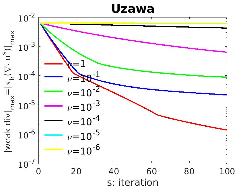
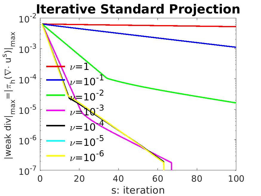
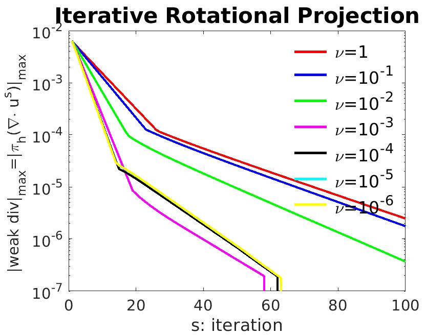
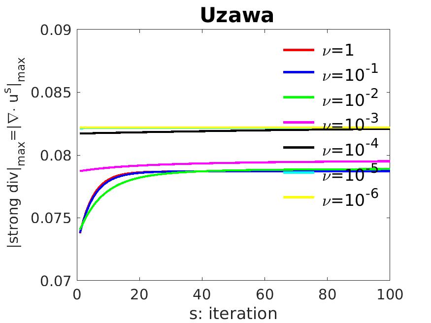
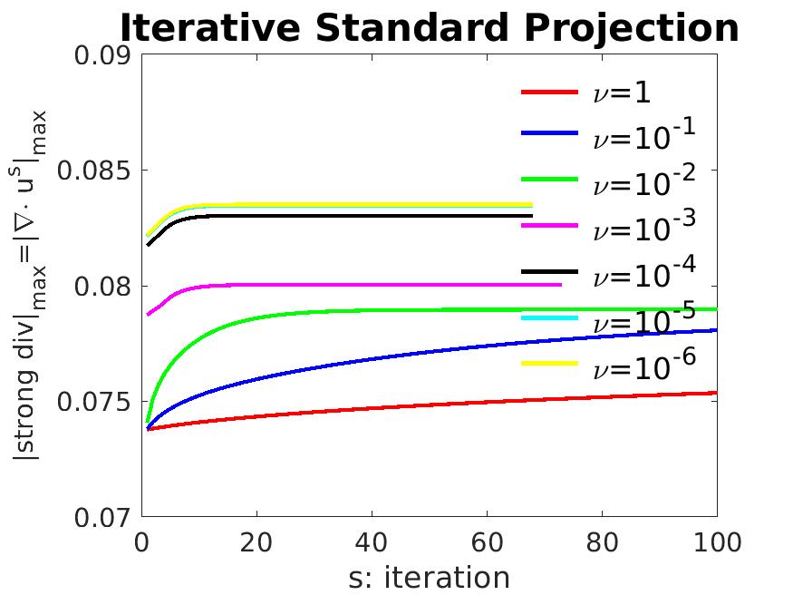
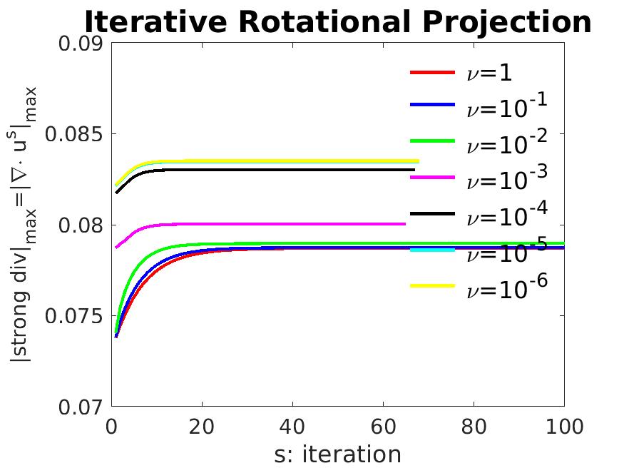
Figure 2: Weak and strong measures of velocity over iterations of Problem 1 in the time step $t=2\times 10^{-3}$ with SI-SKEW convection, $N=80$, $k=10^{-3}$. First row: weak measure. Second row: strong measure.

4.3 About optimal parameter values of $\alpha$ and $\rho$

The normal mode analysis of Section 2.1 shows that the choice of $\alpha=1.5$ and $\rho=\nu$ results in super convergence when the numerical solution is smooth and the convection is absent. When the numerical velocity has only $H^{1}$ regularity and the convection is present, it is hard to analyze the optimal values of these two parameters. Thus, we use numerical tests to get some clues.

Firstly, we study the effect of parameter values on the iteration convergence at the initial time step $t=0.002$ of Problem 1 with the SI-SKEW convection form and the mesh resolution $N=80$. When $\alpha=1.5$, the convergence is faster as $\rho$ grows from 0 to $2\nu$ when $\nu=1$ and $\nu=0.001$, as shown in Figure 3[ab], with an exception at $\nu=1$, $\rho=2\nu$. A direct comparison between $\nu=1$ and $\nu=0.001$ cases indicates the optimal parameters depend less sensitively on $\rho$ when $\nu$ is small. On the other hand, when $\nu=0.001$ and $\rho=2\nu$, the convergence increases as $\alpha$ goes from 1.5 to 2.4 or 2.6 (Figure 3[c]) and decreases as $\alpha$ continues from 2.6 to 3.0. Thus, the optimal value should be close to 2.5.

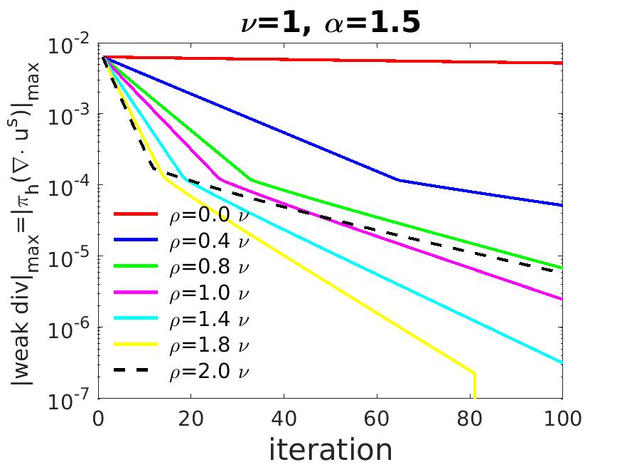
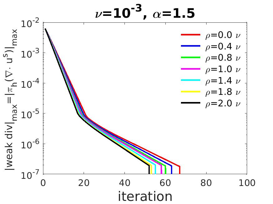
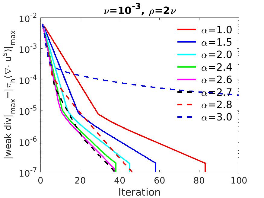
[a] [b] [c]

Figure 3: Effects of $\alpha$ and $\rho$ on iteration convergence in Problem 1 in the time step $t=2\times 10^{-3}$ with SI-SKEW convection, $N=80$, $k=10^{-3}$. [a]: $\nu=1$ and $\alpha=1.5$. [b]: $\nu=10^{-3}$ and $\alpha=1.5$. [c]: $\nu=10^{-3}$ and $\rho=2\nu$.

Secondly, we use the iterative projection method with FI-SKEW convection to solve Problem 1 from $t=0$ to $t=0.5$ with $Re=4600$, $N=60$, and the stopping criterion is $|\text{weak div}|_{\max}<0.01$. We test the speed of the iterative projection method with some different values of $\alpha\in(1,3)$ and $\rho\in[\nu,2\nu]$ and the results are shown in Table 2. All these simulations produce the same error as in the case $N=60$ in Table 8. Note in Table 2, the simulations of the same $\alpha$ value but different $\rho$ values have the identical solution process, which means the $\rho$ choice is not important here. The optimal value of $\alpha$ seems to be close to 2.5 in this particular example, which is consistent with the result from the initial time step test.

Table 2: Effects of parameters $\alpha$ and $\rho$ on iterations of FI-SKEW scheme of evolution of Problem 1

$\alpha$	$\rho$	average iterations
1.5	$\nu$, $1.9\nu$, $2\nu$	9.0
1.9	$\nu$, $1.9\nu$, $2\nu$	6.2
2.0	$\nu$, $1.9\nu$, $2\nu$	6.1
2.5	$\nu$, $1.9\nu$, $2\nu$	5.0
2.8	$\nu$, $1.9\nu$, $2\nu$	6.1

The similar tests are done for Problem 2 mentioned in Section 4.5, where the optimal value occurs around $\alpha=2.9$ and $\rho=2\nu$ when $\nu=10^{-5}$ (data not shown). Based on these numerical tests, we find that the optimal values of parameters to attain the fastest iteration convergence are in the range of $(\alpha,\rho)\in(1.5,3)\times(\nu,2\nu)$ and the specific value depends on the specific problem. It is recommended to test the optimal values at the initial time step with a coarse mesh before running a long time evolution.

4.4 Numerical tests on accuracy of iterative projection method of Problem 1

This group of tests investigates the stability and accuracy of the full scheme (176), (177), and (178) when it is applied to Problem 1. The simulations run from $t=0$ to $t=0.5$ with various Reynolds numbers starting from $Re=920$, where the convergence is evaluated at time $t=0.5$. All the simulations in Section 4.4.1, Section 4.4.2, and Section 4.4.3 use $\alpha=1.5$, $\rho=\nu$, $k=0.001$.

4.4.1 $Re=920$: one iteration attains accurate solutions

In the first case, we choose $Re=920$ and the SI-SKEW convection form. When only one iteration is used, that is, the conventional rotational projection method is employed, the numerical solutions show the optimal convergence (see Table 3): second order accuracy of both the velocity (in $H^{1}$ norm) and the pressure (in $L^{2}$ norm). Therefore, in this case, more than one iteration is not needed. Notably, both the weak and strong incompressibility measures are small (less than 1) as shown in Figure 4.

Table 3: Errors at $t=0.5$ when $Re=920$, iteration=1.

N	$\|{u}_{h}-{u}\|_{H^{1}}$	rate	$|p_{h}-p|_{L^{2}}$	rate
60	$0.20\times 10^{-1}$	1.86	$0.15\times 10^{-4}$	2.01
70	$0.15\times 10^{-1}$	2.32	$0.11\times 10^{-4}$	2.11
80	$0.11\times 10^{-1}$	1.89	$0.83\times 10^{-5}$	2.08
90	$0.88\times 10^{-2}$	2.04	$0.65\times 10^{-5}$	2.12
100	$0.71\times 10^{-2}$		$0.52\times 10^{-5}$

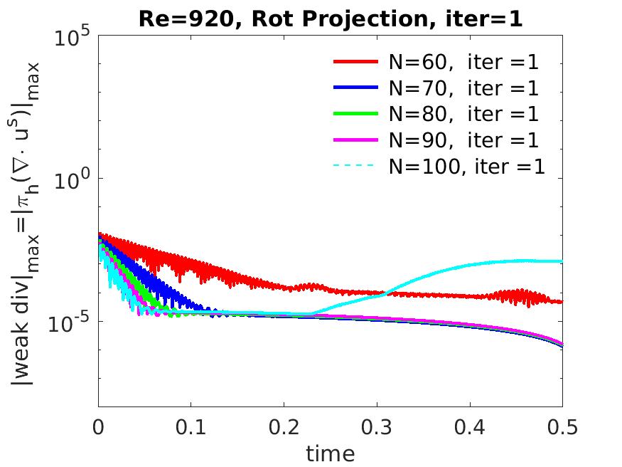
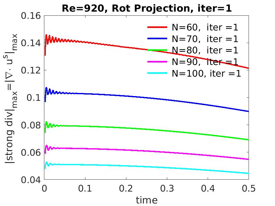
[a] [b]

Figure 4: Weak [a] and strong [b] incompressibility measures for Problem 1 with $Re=920$, iteration=1.

4.4.2 $Re=2300$: iterations reduce/remove spurious solutions

In this subsubsection, all the simulations use the SI-SKEW convection.

1. Only one projection per time step.

   When $Re=2300$, only one projection in every time step leads to large errors when $N=60,70,80$, but delivers accurate solutions when $N=90,100$ (see Table 4). These coincide with sizes of the weak and strong incompressibility measures as shown in Figure 5: when $N=60,70,80$, the measures grow exponentially in time and then stay at high values, but when $N=90,100$, the measures are small (less than 0.1).

   Table 4: Errors at $t=0.5$ when $Re=2300$, iteration=1.

   N	$\|{u}_{h}-{u}\|_{H^{1}}$	rate	$|p_{h}-p|_{L^{2}}$	rate
   60	$0.12\times 10^{+3}$	11	$0.31\times 10^{+1}$	6
   70	$0.42\times 10^{+2}$	33	$0.12\times 10^{+1}$	35
   80	$0.51\times 10^{0}$	33	$0.10\times 10^{-1}$	62
   90	$0.94\times 10^{-2}$	2.14	$0.66\times 10^{-5}$	1.90
   100	$0.75\times 10^{-2}$		$0.54\times 10^{-5}$

   

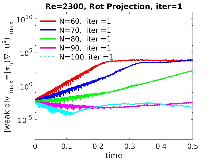
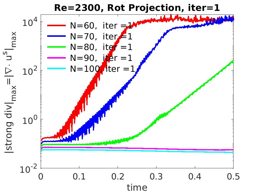
   [a] [b]

   Figure 5: Weak [a] and strong [b] incompressibility measures of Problem 1 when $Re=2300$, iteration=1.

2. Using fixed numbers of iterations per time step.

   To see the effects of iterative projections, we focus on the mesh $N=60$ with a fixed number of iterations per time step: iteration=1, 2, 4, or 6. Based on Table 5, the errors decrease when more iterations are used and when iteration=6, the errors are optimal in the given time and spatial discretizations. The plottings of the numerical solutions in Figure 6 reveal that there are strongly unphysical oscillations when only one iteration is used, but the oscillations reduce when more iterations are added and completely vanish when iteration=6. Correspondingly, both the weak and strong incompressibility measures increase to large values (more than 1000) with respect to time when iteration=1,2,4, but small (less than 0.1) when iteration=6, as illustrated in Figure 7. Especially the strong incompressibility measure shares the same tendency as the $H^{1}$ error of the velocity in the fixed $V_{h}$ space ($h=1/60$) when the iteration number increases, which is an evidence to Remark 4 that the strong incompressibility measure is a marker of spuriousness.

   Table 5: Errors at $t=0.5$ when $Re=2300$, $N=60$, and a fixed number of iterations, “iter”, is applied in each time step.

   $Re$	N	iter	$\|{u}_{h}-{u}\|_{H^{1}}$	$|p_{h}-p|_{L^{2}}$
   2300	60	1	$0.12\times 10^{+3}$	$0.31\times 10^{+1}$
   2300	60	2	$0.43\times 10^{+2}$	$0.13\times 10^{+1}$
   2300	60	4	$0.29\times 10^{+1}$	$0.26\times 10^{-1}$
   2300	60	6	$0.23\times 10^{-1}$	$0.15\times 10^{-4}$

   

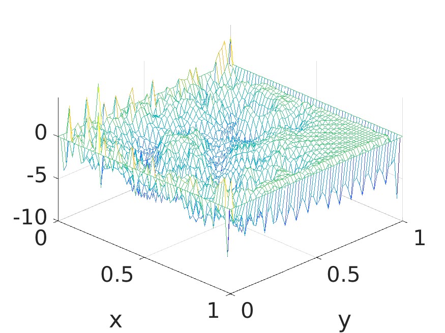
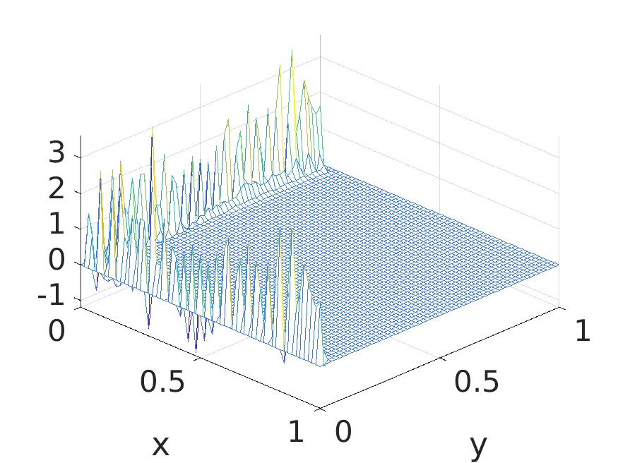
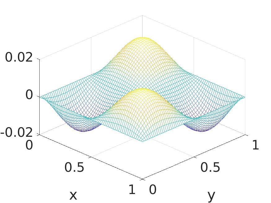
   [a] [b] [c] [d]

   Figure 6: Numerical solution $u_{3}$ on the plane $z=\frac{59}{60}$ of Problem 1 at t=0.5 when $Re=2300$ and $N=60$. Iteration=1 in [a], 2 in [b], 4 in [c], 6 in [d].

   

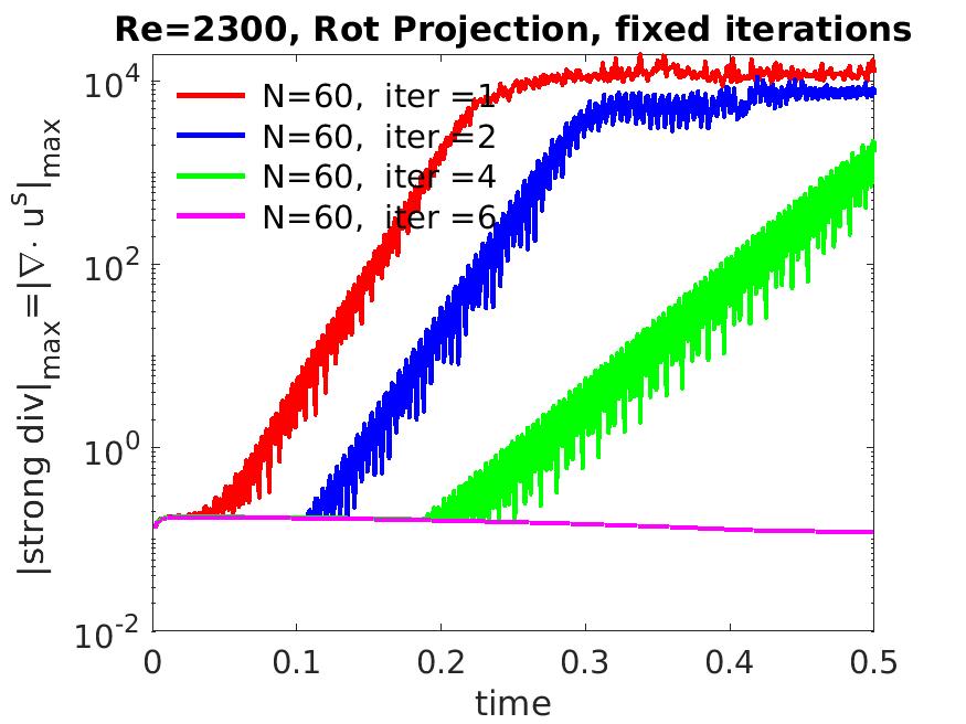
   [a] [b]

   Figure 7: Weak [a] and strong [b] incompressibility measures when $Re=2300$, $N=60$, and iteration=1, 2, 4, 6.

3. Using stopping criterion in formula (266)

   One apparent issue of using a fixed number of iterations in every time step is that the smallest number of iterations sufficient for removing spurious modes is unknown before simulations. Therefore, we switch the stopping criterion (266) with $\epsilon=10^{-2}$ and re-run the simulations of Problem 1 with $Re=2300$. The optimal convergence is recovered as shown in Table 6. Both the weak and strong incompressibility measures are small, according to Figure 8.

   Table 6: Errors at $t=0.5$ when $Re=2300$ and the stopping criterion is (266) with $\epsilon=10^{-2}$. “average iter” is the average iteration in all the time steps.

   N	$\|{u}_{h}-{u}\|_{H^{1}}$	$|p_{h}-p|_{L^{2}}$	average iter
   60	$0.23\times 10^{-1}$	$0.15\times 10^{-4}$	5.2
   70	$0.16\times 10^{-1}$	$0.11\times 10^{-4}$	3.5
   80	$0.12\times 10^{-1}$	$0.83\times 10^{-5}$	1.7
   90	$0.94\times 10^{-2}$	$0.66\times 10^{-5}$	1
   100	$0.75\times 10^{-2}$	$0.53\times 10^{-5}$	1

   

   

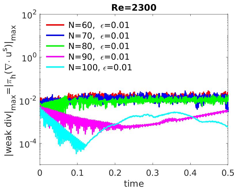
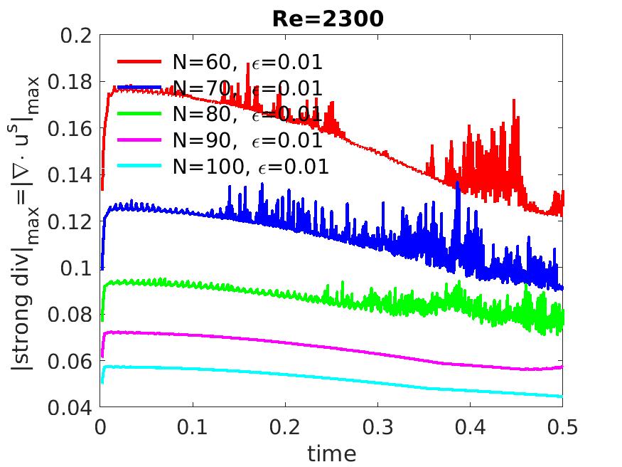
   Figure 8: Weak [a] and strong [b] incompressibility measures of Problem 1 when $Re=2300$ and the stopping criterion is (266) with $\epsilon=10^{-2}$.

4.4.3 $Re=4600$: semi-implicit vs fully-implicit schemes

1. SI-SKEW-based iterative projection method.

   When the Reynolds number increases to $Re=4600$, we first employ the SI-SKEW convection and set the stopping criterion as (266) with $\epsilon=10^{-7}$. The numerical solutions show a strange behavior. The standard exact solution of $u_{1}$ of Problem 1 is zero on the plane $z=0.5$ at all time, but the numerical solution is nonzero, as shown in Figure  9. This solution is spurious but the magnitude of oscillation is much smaller than what are presented in Figure 6 when iteration=1. In addition, when the mesh is refined from $N=60$ to $N=100$, the numerical solution converges to that at $N=100$ for both the velocity and pressure in $L^{2}$ norm, as shown in Table 7. The velocity error with respect to the exact solution and the strong incompressibility measure are shown in Figure 10[ab]. Both surge suddenly from less than one to some large values at certain time steps between $t=0.2$ and $t=0.4$ for all these simulations. This further confirms the role of the strong measure as the marker of the spuriousness of numerical solutions.

   

   

   

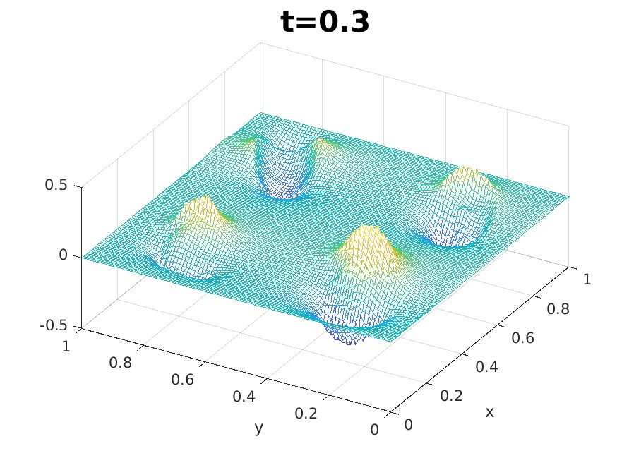
   Figure 9: Numerical solutions of $u_{1}$ on the $z=0.5$ plane of Problem 1 at $t=0.25,0.3,0.5$. Parameters: $Re=4600$, $N=100$, and $k=10^{-3}$. The standard exact solution $u_{1}$ is zero on this plane. The SI-SKEW convection is used.

   Table 7: Difference between the numerical solution with mesh resolution $N<100$ and that of $N=100$. $Re=4600$. The SI-SKEW convection is used. Stopping criterion is (266) with $\epsilon=10^{-7}$.

   N	$\|u_{N}-u_{100}\|_{L^{\infty}(0,0.5;L^{\infty}\Omega)}$	$\|u_{N}-u_{100}\|_{L^{2}(0,0.5;L^{2}\Omega)}$	$||p_{N}-p_{100}||_{L^{2}(0,0.5;L^{2}\Omega)}$	average iter
   60	$0.25769\times 10^{+1}$	$0.19696\times 10^{0}$	$0.17290\times 10^{0}$	15.0
   70	$0.25764\times 10^{+1}$	$0.15761\times 10^{0}$	$0.13233\times 10^{0}$	17.7
   80	$0.26592\times 10^{+1}$	$0.11724\times 10^{0}$	$0.95676\times 10^{-1}$	21.4
   90	$0.23662\times 10^{+1}$	$0.71958\times 10^{-1}$	$0.57587\times 10^{-1}$	27.9
   96	$0.29156\times 10^{+1}$	$0.44540\times 10^{-1}$	$0.28873\times 10^{-1}$	25.0
   97	$0.19185\times 10^{+1}$	$0.41189\times 10^{-1}$	$0.26961\times 10^{-1}$	25.6
   98	$0.19823\times 10^{+1}$	$0.40630\times 10^{-1}$	$0.27062\times 10^{-1}$	26.4
   99	$0.21280\times 10^{+1}$	$0.35669\times 10^{-1}$	$0.21571\times 10^{-1}$	25.5

   

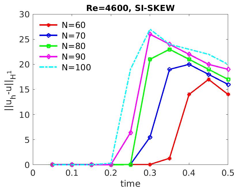
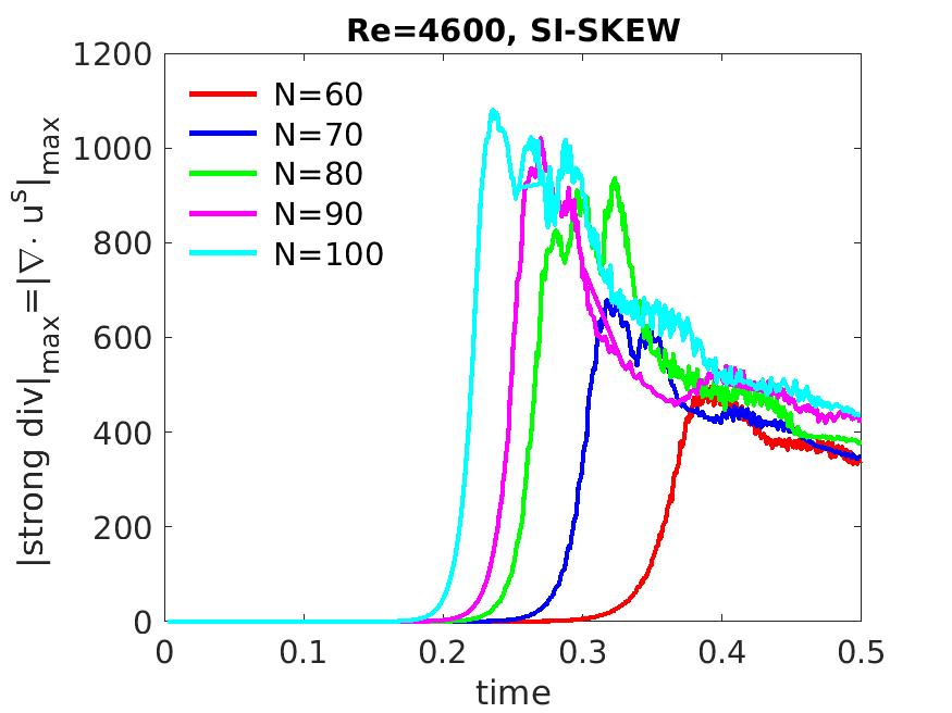
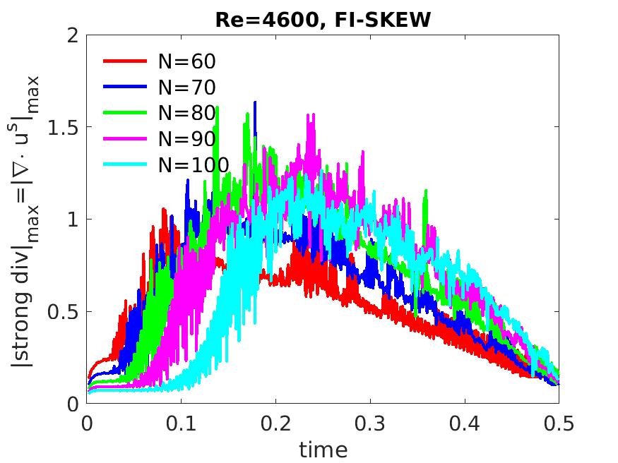
   [a] [b] [c]

   Figure 10: [a,b]: velocity error [a] and strong incompressibility measure [b] of SI-SKEW with $Re=4600$. [c]: strong incompressibility measure of FI-SKEW when $Re=4600$. The stopping criterion is (266) with $\epsilon=10^{-2}$ in [abc].

   The direct reason for this false numerical solution for the iterative SI-SKEW scheme is that at a certain time step, the weak incompressibility measure cannot converge to zero given sufficient iterations although this measure can be very small. For example, when $N=100$, the weak incompressibility measure is stuck at $1.1067\times 10^{-7}$ at iteration steps from 22 to 50 at time step $t=0.219$, the moment when the strong incompressibility measure suddenly rises to a high value in Figure 10[b]. Therefore, the iterative projection method fails to converge at this time step.

2. FI-SKEW-based iterative projection method

   When the FI-SKEW form is adopted and the stopping criterion is (266) with $\epsilon=10^{-2}$, the correct solution is recovered as shown in Table 8. This suggests the fully implicit scheme is more robust than the semi-implicit scheme under the same setting and a possible reason is that the fully implicit scheme preserves better the nonlinear structure of the original Navier-Stokes equations.

   A side note is that although the acceleration technique mentioned in Appendix B can speed up the iteration convergence in many simulations including the cases $N=60,80,90$ in Table 8, it is not guaranteed to always produce convergence. For instance, when $N=70$, the iteration using this acceleration blows up at time $t=0.489$. More studies are required to uncover the conditions to apply the acceleration techniques.

   Table 8: Errors when $Re=4600$ and the stopping criterion is (266) with $\epsilon=10^{-2}$. The convection is FI-SKEW.

   N	$||{u}_{h}-{u}||_{H^{1}}$	rate	$|p_{h}-p|_{L^{2}}$	rate	average iter
   60	$0.29\times 10^{-1}$	2.4	$0.18\times 10^{-4}$	2.6	9.0
   70	$0.20\times 10^{-1}$	2.2	$0.12\times 10^{-4}$	1.4	6.5
   80	$0.15\times 10^{-1}$	2.6	$0.10\times 10^{-4}$	3.3	5.1
   90	$0.10\times 10^{-1}$	2.1	$0.68\times 10^{-5}$	0.6	3.9
   100	$0.88\times 10^{-2}$		$0.64\times 10^{-5}$		2.4

4.4.4 Some higher Reynolds numbers

This set of simulations applies the iterative projection method with the FI-SKEW convection term to handle some high Reynolds numbers $Re=5\times 10^{3}$, $10^{4}$, $2\times 10^{4}$, $4\times 10^{4}$ of Problem 1, and the stopping criterion is (266) with $\epsilon=10^{-2}$. The computational results are shown in Figure 11. Both the $L^{2}$ and $H^{1}$ errors of velocity are optimal and increase when the Reynolds number is larger, which is consistent with the non-robust error estimates of this non-div-free FEM. The average iterations per time step also increase with the Reynolds numbers and are below 9 in these simulations.

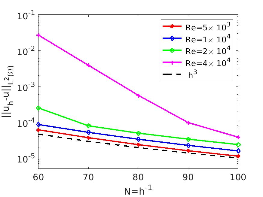
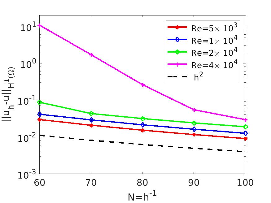
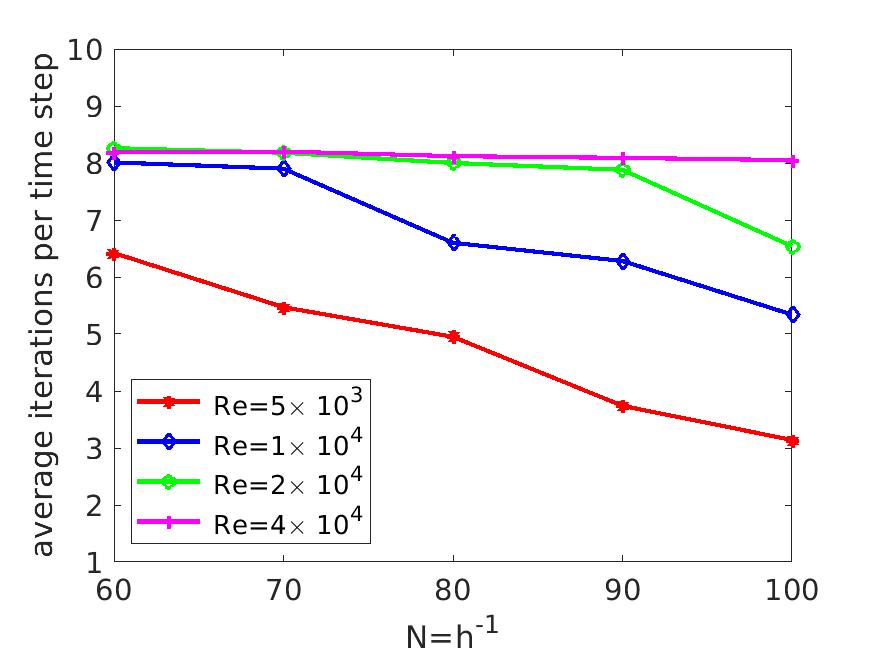
[a] [b] [c]

Figure 11: Simulation results for Problem 1 with FI-SKEW convection and the stopping criterion is (266) with $\epsilon=10^{-2}$. [ab]: $L^{2}$ and $H^{1}$ errors of velocity. [c]: average iteration numbers per time step.

4.4.5 Comparison with iterative IMEX projection scheme

Following [3], we use a BDF2-IMEX scheme, where the only difference with the method proposed in this work ((176), (177), and (178)) is that the equation (176) is replaced by

$$1.5(u_{h}^{n+1,s},v_{h}) +k\nu(\nabla u_{h}^{n+1,s},\nabla v_{h})-k(\nabla\cdot v_{h},p^{n+1,s}_{h})$$

$$=(2u^{n}_{h}-0.5u^{n-1}_{h},v_{h})+k(f^{n+1},v_{h})-k((w^{n+1}_{h}\cdot\nabla)w^{n+1}_{h},v_{h}),$$ (272)

where $w^{n+1}_{h}=2u^{n}_{h}-u^{n-1}_{h}$. That is, the diffusion term $\nu(\nabla u_{h}^{n+1,s},\nabla v_{h})$ is implicit but the convection term $((w^{n+1}_{h}\cdot\nabla)w^{n+1}_{h},v_{h})$ is completely explicit. Using the same proof for Theorem 1, with $f$ replaced with $f-(w^{n+1}_{h}\cdot\nabla)w^{n+1}_{h}$ in (30), it is easy to see that when $s\to\infty$, the scheme converges to the following system,

$$1.5(u_{h}^{n+1},v_{h}) +k\nu(\nabla u_{h}^{n+1},\nabla v_{h})-k(\nabla\cdot v_{h},p^{n+1}_{h})=(2u^{n}_{h}-0.5u^{n-1}_{h},v_{h})$$

$$+k(f^{n+1},v_{h})-k((w^{n+1}_{h}\cdot\nabla)w^{n+1}_{h},v_{h}),\quad\forall v_{h}\in V_{h},$$ (273)

$$(\nabla\cdot u^{n+1}_{h},q_{h}) =0,\quad\forall q_{h}\in Q_{h}.$$ (274)

For this scheme, it is impossible to prove an energy estimate similar to Theorem 4. Indeed, letting $v_{h}=u^{n+1}$ in (273) and $q_{h}=p^{n+1}_{h}$ in (274), we obtain

$$\,\|u^{n+1}_{h}\|^{2}_{L^{2}_{x}}+\|2u^{n+1}_{h}-u^{n}_{h}\|^{2}_{L^{2}_{x}}+\|u^{n+1}_{h}-2u^{n}_{h}+u^{n-1}_{h}\|^{2}_{L^{2}_{x}}+4k\nu\|\nabla u^{n+1}_{h}\|^{2}_{L^{2}_{x}}$$

$$= \,\|u^{n}_{h}\|^{2}_{L^{2}_{x}}+\|2u^{n}_{h}-u^{n-1}_{h}\|^{2}_{L^{2}_{x}}+4k(f^{n+1},u^{n+1}_{h})-4k((w^{n+1}_{h}\cdot\nabla)w^{n+1}_{h},u^{n+1}_{h}).$$ (275)

Following a process similar to that used to derive (94) and (95), we can get

$$|4k((w^{n+1}_{h}\cdot\nabla)w^{n+1}_{h},u^{n+1}_{h})|\leq \,4k\|w^{n+1}_{h}\|_{L^{4}_{x}}\|u^{n+1}_{h}\|_{L^{4}_{x}}\|\nabla w^{n+1}_{h}\|_{L^{2}_{x}}$$

$$\leq \,8k\|w^{n+1}_{h}\|^{\frac{1}{4}}_{L^{2}_{x}}\|\nabla w^{n+1}_{h}\|^{\frac{3}{4}}_{L^{2}_{x}}\|u^{n+1}_{h}\|^{\frac{1}{4}}_{L^{2}_{x}}\|\nabla u^{n+1}_{h}\|^{\frac{3}{4}}_{L^{2}_{x}}\|\nabla w^{n+1}_{h}\|_{L^{2}_{x}}.$$ (276)

By the Poincaré inequality, $\|w^{n+1}_{h}\|_{L^{2}_{x}}\leq C\|\nabla w^{n+1}_{h}\|_{L^{2}_{x}}$ and $\|u^{n+1}_{h}\|_{L^{2}_{x}}\leq C\|\nabla u^{n+1}_{h}\|_{L^{2}_{x}}$. Then (276) becomes

$$|4k((w^{n+1}_{h}\cdot\nabla)w^{n+1}_{h},u^{n+1}_{h})|\leq kC\|\nabla(2u^{n}_{h}-u^{n-1}_{h})\|^{2}_{L^{2}_{x}}\|\nabla u^{n+1}_{h}\|_{L^{2}_{x}}.$$ (277)

This nonlinear term makes it impossible to derive a recursive relation from (275). Similarly, the error estimate for (273) and (274), by following the same process as in the proof of Theorem 5, generates one term $(((2\phi^{n}_{h}-\phi^{n-1}_{h})\cdot\nabla)(2\phi^{n}_{h}-\phi^{n-1}_{h}),\phi^{n+1}_{h})$. Using the same argument as in (276) and (277), we can obtain its upper bound as $C\|\nabla(2\phi^{n}_{h}-\phi^{n-1}_{h})\|^{2}_{L^{2}_{x}}\|\nabla\phi^{n+1}_{h}\|_{L^{2}_{x}}$. With the same reason for the stability, it is also impossible to derive a recursive relation for the error analysis.

The numerical simulations further suggest this iterative IMEX projection scheme is not so stable as the proposed scheme ((176), (177), and (178)). When $Re=920$ and $k=0.001$, this scheme blows up around $t=0.1$ (see Figure 12). In contrast, the iterative SI-SKEW scheme obtains the optimal convergence with just one iteration in each time step according to Section 4.4.1.

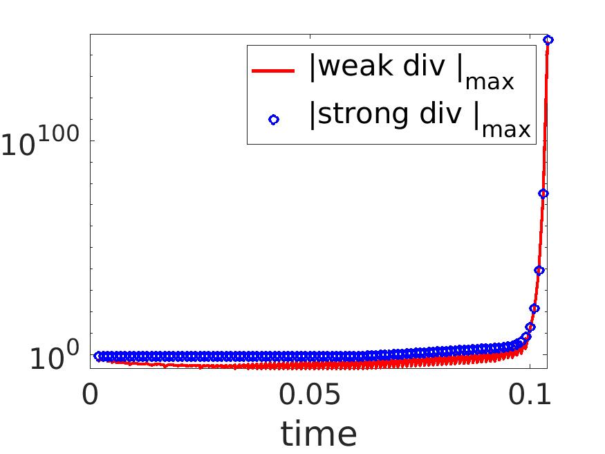
Figure 12: Weak and strong incompressibility measures when iterative IMEX method is used in Problem 1 with $Re=920$ and $k=0.001$. The stopping criterion is (266) with $\epsilon=10^{-7}$.

4.5 Problem 2: iterative projection method in lid driven cavity flow

Problem 2 is a classic lid driven cavity problem. The domain is $\Omega=(-0.5,0.5)^{3}$ and the velocity is ${u}=(0,1,0)$ on the wall $x=-0.5$ and zero on the other walls. The initial velocity is set as zero everywhere except on the sliding wall. The meshes use Gauss-Lobatto points (e.g. [2]), where $x_{i}=0.5\cos(\frac{i\pi}{N})$, $y_{j}=0.5\cos(\frac{j\pi}{N})$, $z_{l}=\frac{l\pi}{N}-0.5$, $i,j,l=0,\cdots,N$, where $N$ is the number of subdivisions in each direction. The Reynolds number of this problem is $Re=\frac{1}{\nu}$.

We run the simulations with the SI-SKEW convection form, $\nu=0.001$ or $Re=1000$, $\alpha=1.5$, $\rho=\nu$, and $k=0.001$. The simulations are run until the velocity reaches a steady state. Since the exact solution is not available, the solution at $t_{1}$ is taken the same as $t_{0}=0$. The solution at $t_{2}$ is obtained by running the scheme until it converges.

When $N=40$, the conventional rotational projection method shows very chaotic velocity and pressure fields at $t=1$, as shown in Figure 13. But when two projection iterations are used in each time step, the velocity field looks very smooth (Figure 14).

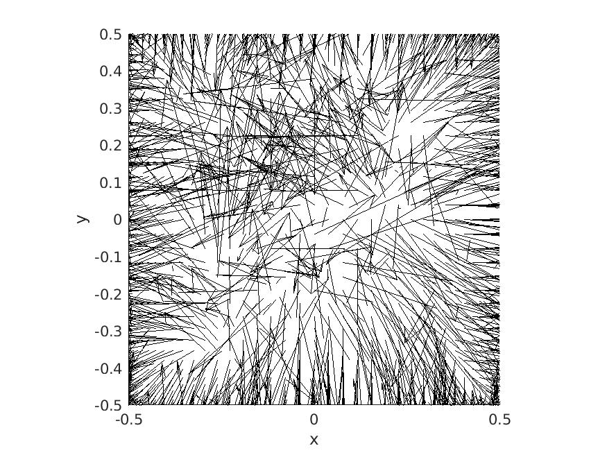
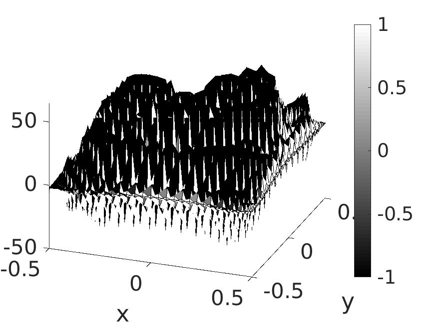
[a] [b]

Figure 13: Velocity[a] and pressure[b] on the x-y plane of $z=0$, at time $t=1$. $Re=1000$, iteration=1, max speed=22.79.

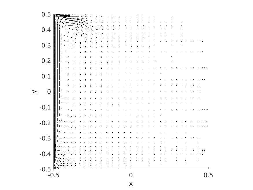
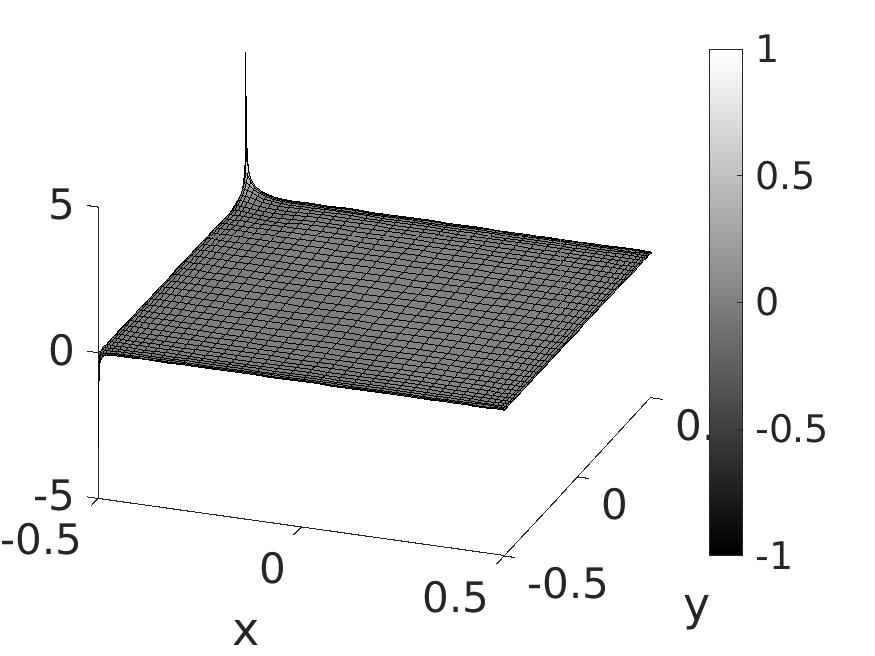
[b] [b]

Figure 14: Velocity[a] and ressure[b] on the x-y plane of $z=0$ at time $t=1$. $Re=1000$, iteration=2, max speed=1.

The accuracy of the numerical solution is confirmed by the agreement with the results of [2] as shown in Figure 15 when the mesh is refined from $N=20$ to $N=40$ and iteration=2 in each time step. In [2], the standard projection scheme with BDF2 scheme in time and spectral method in space is used. More importantly, they construct a special solution $u_{c}$ addressing the edge singularity to accompany the numerical solution. Therefore, without introducing the prescribed singular solution, the proposed iterative projection method obtains the correct solution with just two projections in each time step.

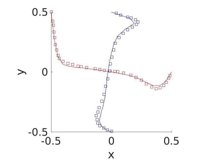
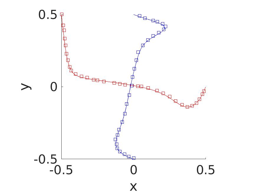
[a] [b]

Figure 15: Comparison of normalized velocities, $v/2$ and $u/2$ (the whole velocity vector is $(u,v,w)$) with those in [2], on the center lines $(x,0,0)$ and $(0,y,0)$ on the x-y plane $z=0$ in the cubic cavity flow. The square symbols are extracted from figures of [2]. The solid lines are from the iterative projection method of this work. [a]: $N=20$. [b]: $N=40$. The Reynolds number $Re=1000$. The time is $t=20$.

5 Summary

This work introduces an iterative projection method for the Navier-Stokes equations, whose methodology is to iterate the classic projection method in every time step with a proper convection form to guarantee stability. The benefits are tremendous. First, when fully convergent, it produces the weakly divergence free velocity (and almost everywhere divergence free velocity on divergence free finite element methods). Second, the stability and error estimates are theoretically established when the projection iterations are convergent in every time step. Third, this method can handle high Reynolds numbers. When the finite element spaces are divergence free, this method is robust, that is, the error estimate of velocity in $L^{2}$ norm is independent of the viscosity or Reynolds numbers. When the projection iterations are not fully convergent, the numerical experiments show that the method can still preserve stability and accuracy for high Reynolds numbers. All these properties are absent in the classic projection method. At the same time, this new approach keeps an essential property of the classic projection method: the splitting of the velocity and pressure fields, which results in the splitting of a large saddle point system into small elliptic problems.

A condition to warrant the iteration convergence with two parameters is derived, as shown in Theorem 2 and Theorem 3. A range of the parameter values to achieve the fast iteration convergence is given in Section 4.3. Two incompressibility measures are proposed to track the performance of numerical solutions. The weak measure monitors whether the iterations are convergent or not and the strong measure indicates whether the numerical solution is spurious or not. These two measures are equivalent for the div-free FEMs but not for the non-div-free FEMs. Under the non-div-free FEMs, if the weak measure is small but strong measure is too large, the numerical solution would be non-physical. In this work, both the semi-implicit and the fully implicit skew-symmetric convection forms are studied and tested. The numerical simulations show that the fully implicit scheme is more stable and accurate and efficient than the semi-implicit form.

Note it is the limit scheme, the one achieved when the iterative projections are convergent in each time step, that endows this method the properties such as stability, accuracy, and robustness to Reynolds numbers. Thus, there are many ways this work can be improved and extended. First, the scheme proposed in this work does not use any stabilization techniques mentioned in [14]. A simple and appealing stabilization is the grad-div method as mentioned in [11], also used in the augmented Lagrangian method [13], which has been shown to achieve robust error estimates for non-div-free FEMs. Second, there are many other forms of the convection term as shown in [9], whose theoretical and computational properties can be studied. Third, the convergence rate of the projection iterations for (4) and (5) is first order, and its comparison in efficiency with Newton’s method with GMRES approach of solving the nonlinear system as in [9] will be an interesting future work.

Finally, this iterative projection method is a completely new and efficient numerical method for the saddle point problem from the discretization of the time dependent Navier-Stokes equations. It is an extension of the Uzawa method by adding only one Poisson equation in the pressure space, which is from the Hodge decomposition of the intermediate velocity. The same as the Uzawa method, the method has a linear convergence rate. However, normal mode analysis and numerical experiments reveal that with proper parameters, the iterative projection method is much faster than the Uzawa method when the viscosity is small or the Reynolds number is large. Because the Uzawa method is a popular method for many saddle point problems including the Stokes equations and steady Navier-Stokes equations, it is worthwhile to consider whether this method can be extended to these saddle point problems.

Appendix A One-step projection does not produce divergence free velocity

Using the matrix and vector notations in Section 2.2.1, the equation (9) and (11) can be written as

$$G\vec{\phi}^{n+1} =\frac{1}{k}B\vec{u}^{*},$$ (A.1)

$$A_{0}\vec{u}^{n+1} =A_{0}\vec{u}^{*}-kB^{T}\vec{\phi}^{n+1}.$$ (A.2)

where $A_{0}$ is the mass matrix of $V_{h}$. That is, $(A_{0})_{ij}=(w_{i},w_{j})$, $i,j=1,\cdots,l$. These two equations yield

$$B\vec{u}^{n+1}=(I-BA_{0}^{-1}B^{T}G^{-1})(B\vec{u}^{*}).$$ (A.3)

In general, $BA_{0}^{-1}B^{T}=G$ does not hold for mixed finite element spaces. Thus, $I-BA_{0}^{-1}B^{T}G^{-1})\neq 0$ and $B\vec{u}^{n+1}\neq 0$. This implies $u^{n+1}$ is not weakly divergence free in the traditional one-step projection method.

Appendix B An acceleration technique

As in [3], acceleration techniques based on Aitken method can be applied to the iterations in this work. There are many variants of Aitken’s method and we use the following one (Method 3 of [22]). Denote $f$ as an algorithm generating a fixed point $p$ of $f$, i.e., $p=f(p)$. Given an initial guess $p_{0}$, the non-accelerated algorithm produces a sequence $\{p_{s}\}$ with the relation $p_{s}=f(p_{s-1})$, $s=1,2,\cdots$. In the accelerated scheme, the new sequence is generated as follows. With an initial guess $p_{0}$, let $p_{1}=f(p_{0})$ and $p_{s}$, $s\geq 2$, be as follows,

$$p_{s} = f(p_{s-1})+\mu_{k}(p_{s-1}-f(p_{s-1})),$$ (B.1)

$$\text{ where }\quad\mu_{k} = \frac{(r_{s},r_{s}-r_{s-1})}{\|r_{s}-r_{s-1}\|^{2}},\quad r_{s-1}=f(p_{s-2})-p_{s-2},\quad r_{s}=f(p_{s-1})-p_{s-1}.$$ (B.2)

A comparison is given for the iterations in the first time step between non-accelerated and accelerated schemes for Problem 1 with the rotational projection scheme and SI-SKEW convection form. The parameters used are $\nu=10^{-5}$, $N=80$, time step size $k=10^{-3}$. The results are shown in Figure B.1. In this example, the accelerated scheme saves about one half iterations as of the non-accelerated one.

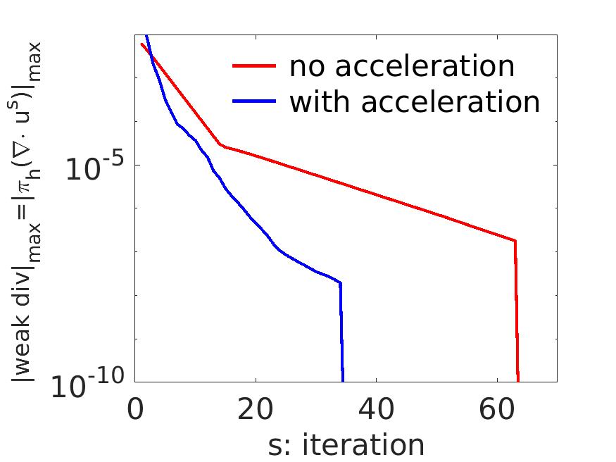
Figure B.1: Comparison of iterations between accelerated and non-accelerated schemes.

References

- [1] N. Ahmed, C. Bartsch, V. John, and U. Wilbrandt. An assessment of some solvers for saddle point problems emerging from the incompressible Navier–Stokes equations. Computer Methods in Applied Mechanics and Engineering, 331:492–513, 2018.
- [2] S. Albensoeder and H.C. Kuhlmann. Accurate three-dimensional lid-driven cavity flow. Journal of Computational Physics, 206(2):536 – 558, 2005.
- [3] J. Aoussou, J. Lin, and P.F.J. Lermusiaux. Iterated pressure-correction projection methods for the unsteady incompressible Navier–Stokes equations. Journal of Computational Physics, 373:940–974, 2018.
- [4] K. Arrow, L. Hurwicz, and H. Uzawa. Studies in Linear and Nonlinear Programming. Stanford University Press, 1958.
- [5] M. Benzi, G.H. Golub, , and J. Liesen. Numerical solution of saddle point problems. Acta Numerica, 14:1–137, 2005.
- [6] S.C. Brenner and L.R. Scott. The Mathematical Theory of Finite Element Methods. Springer, third edition, 2008.
- [7] D.L. Brown, R. Cortez, and M.L. Minion. Accurate projection methods for the incompressible Navier-Stokes equations. Journal of Computational Physics, 168:464–499, 2001.
- [8] M. Cai. Analysis of some projection method based preconditioners for models of incompressible flow. Applied Numerical Mathematics, 90:77–90, 2015.
- [9] S. Charnyi, T. Heister, M.A. Olshanskii, and L.G. Rebholz. On conservation laws of Navier–Stokes Galerkin discretizations. Journal of Computational Physics, 337:289–308, 2017.
- [10] A.J. Chorin. Numerical solution of the navier–stokes equations. Mathematics of Computation, 22:745–762, 1968.
- [11] J. de Frutos, B. García-Archilla, V. John, and J. Novo. Analysis of the grad-div stabilization for the time-dependent Navier-Stokes equations with inf-sup stable finite elements. Advances in Computational Mathematics, 44:195–225, 2018.
- [12] C. Doering, J. Wu, K. Zhao, and X. Zheng. Long time behavior of the two-dimensional boussinesq equations without buoyancy diffusion. Physics D: Nonlinear Phenomena, 376-377:144–159, 2018.
- [13] M. Fortin and R. Glowinski. Augmented Lagrangian Methods, Applications to the Numerical Solution of Boundary-Value Problems. North Holland, 1983.
- [14] B. Garcia-Archilla, V. John, and J. Novo. On the convergence order of the finite element error in the kinetic energy for high reynolds number incompressible flows. Computer Methods in Applied Mechanics and Engineering, 385:114032, 2021.
- [15] B. Griffith. An accurate and efficient method for the incompressible navier–stokes equations using the projection method as a preconditioner. Journal of Computational Physics, 228:7565–7595, 2009.
- [16] J.L. Guermond, C. Migeon, G. Pineau, and L. Quartapelle. Start-up flows in a three-dimensional rectangular driven cavity of aspect ratio 1:1:2 at Re = 1000. Journal of Fluid Mechanics, 450:169–199, 2002.
- [17] J.L. Guermond, P. Minev, and J. Shen. An overview of projection methods for incompressible flows. Computer Methods in Applied Mechanics and Engineering, 195(44):6011 – 6045, 2006.
- [18] J.L. Guermond and L. Quartapelle. On stability and convergence of projection methods based on pressure poisson equation. International Journal for Numerical Methods in Fluids, 26:1039–1053, 1998.
- [19] J.L. Guermond and J. Shen. On the error estimates for the rotational pressure-correction projection methods. Mathematics of Computation, 73:1719–1737, 2004.
- [20] R. Horn and C. R. Johnson. Matrix Analysis. Cambridge University Press, second edition, 2013.
- [21] P. Keast. Moderate-degree tetrahedral quadrature formulas. Computer Methods in Applied Mechanics and Engineering, 55(3):339–348, 1986.
- [22] A. Macleod. Acceleration of vector sequences by multi-dimensional delta2 methods. Communications in Applied Numerical Methods, 2(4):385–392, 1986.
- [23] M.A. Olshanskii and L.G. Rebholz. Longer time accuracy for incompressible Navier–Stokes simulations with the EMAC formulation. Computer Methods in Applied Mechanics and Engineering, 372:113369, 2020.
- [24] Y. Saad. ILUT: A dual threshold incomplete LU factorization. Numerical Linear Algebra with Applications, 1(4):387–402, 1994.
- [25] Y. Saad and M.H. Schultz. GMRES: A Generalized Minimal Residual Algorithm for Solving Nonsymmetric Linear Systems. SIAM Journal on Scientific and Statistical Computing, 7:856–869, 1986.
- [26] P.W. Schroeder and G. Lube. Pressure-robust analysis of divergence-free and conforming FEM for evolutionary incompressible Navier–Stokes flows. Journal of Numerical Mathematics, 25(4):249–276, 2017.
- [27] L.R. Scott and M. Vogelius. Conforming finite element methods for incompressible and nearly incompressible continua. In Lectures in Applied Mathematics, volume 22, pages 221–244. 1984.
- [28] R. Temam. Une méthode d’approximation de la solution des équations de Navier-Stokes. Bulletin de la Société Mathématique de France, 96:115–152, 1968.
- [29] R. Temam. Navier-Stokes Equations: Theory and Numerical Analysis. AMS Chelsea Publishing, 1984.
- [30] L.J.P. Timmermans, P.D. Minev, and F.N. Van De Vosse. An approximate projection scheme for incompressible flow using spectral elements. International Journal for Numerical Methods in Fluids, 22(7):673–688, 1996.
- [31] X. Zheng, J. Lowengrub, A. Anderson, and V. Cristini. Adaptive unstructured volume remeshing-ii: Applications to two- and three-dimensional levelset simulations of multiphase flow. Journal of Computational Physics, 208:625–650, 2005.