Dynamics of the driven open double two-level system and its entanglement generation

Abstract

We investigate the dynamics of the driven open double two-level system by deriving a driven-Markovian master equation based on the Lewis-Riesenfeld invariants theory. The transitions induced by coupling to the heat reservoir occur between the instantaneous eigenstates of the Lewis-Riesenfeld invariant. Therefore, different driving protocols associated with corresponding Lewis-Riesenfeld invariants result in different open system dynamics and symmetries. In particular, we show that, since the instantaneous steady state of the driven double two-level system is one of eigenstates of the Lewis-Riesenfeld invariant at ultra-low reservoir temperature, the inverse engineering method based on the Lewis-Riesenfeld invariants has a good performance in rapidly preparing quantum state of open quantum systems. As an example, a perfect entangled state is generated by means of the inverse engineering method.

I Introduction

The quantum control aims at manipulating the quantum system into desired quantum states or achieving certain quantum operations with satisfied fidelity by using limited control manners. To improve the performance of the quantum control, the dynamics of the quantum system has to be described as exactly as possible. If the quantum system is isolated, its dynamics is governed by the Schrödinger equation, which results in a unitary evolution. Based on the exact dynamical equation of the isolated systems, many effective methods are proposed, such as the adiabatic controlKral2007 ; Hatomura2021 , the shortcuts to adiabaticityOdelin2019 ; Campo2019 , the optimal controlWerschnik2007 and the Lyapunov controlHou2012 ; Yi2009 . However, any system in nature unavoidably couples to its surroundings. Therefore, the system in the real world is never isolated, but an open systemBreuer2007 . There are many different methods for describing dynamics of different open quantum systems, such as the Markovian master equationDavies1974 ; Davies1978 , the quantum state diffusion equationFlannigan2022 and the stochastic Schrödinger equationBouten2004 .

The master equation method gets special attention due to its concise expression and clear physical meaningsBreuer2007 . To formulate the reduced dynamics of open quantum systems, one needs to trace out the degree of freedom of the environment. In the original derivation of the Markovian master equation, it is assumed that the system Hamiltonian is static. The coupling with the environment induces transitions between the static eigenstates of the system HamiltonianLindblad1976 ; Gorini1976 . But this master equation cannot be used to describe the dynamics of the open systems with time-dependent external drives. Many efforts have been devoted to develop the dynamical equation of the driven open quantum systems. For the driving protocols fulfilling the adiabatic condition, the master equation in the adiabatic limit is easy to be formulated Davies1978 ; Albash2012 ; Childs2001 ; Kamleitner2013 ; Sarandy2004 , since the unitary transformation associated with the system Hamiltonian can be given explicitly by the instantaneous eigenstates of the system Hamiltonian. However, beyond the adiabatic limit, it is difficult to give a general master equation without any restriction on the driving protocolYamaguchi2017 ; Dann2018 ; Potts2021 . Even for the simplest two-level system, deriving a non-adiabatic Markovian master equation is a nontrivial taskDann2020 , let alone multi-level systems.

Recently, based on the Lewis-Riesenfeld invariants (LRI) theoryLewis1968 ; Lewis1969 , a method of deriving the Markovian master equation for the driven open quantum systems has been proposed, which is known as the driven Markovian master equation (DMME)Wu2022 . The DMME can be used to describe the open system dynamics with arbitrary control protocols under the Born-Markovian approximation. In this paper, we derive the DMME for a driven double two-level system coupled to a common heat reservoir. We show that the transition induced by the decoherence occurs between the eigenstates of the LRI but not the system Hamiltonian’s. And the decoherence-free subspaces still emerge in the dynamicsKarasik2008 ; Wu2017 . Moreover, if the environment is a vacuum reservoir, the instantaneous steady state is one of eigenstates of the invariant. Therefore, the inverse engineering method based on the Lewis-Riesenfeld invariants may present a high performance in this eigenstateChen2010 ; Chen2011 ; Herrera2014 . We verify this observation by proposing a protocol to generate a maximally entangled state with a perfect fidelity. Since the decoherence always draw a quantum state into the instantaneous steady state (the eigenstate used in the inverse engineering), our control protocol is also robust to the imperfect initial state preparation. Hence, the inverse engineering method is more robust to the decoherence than pervious predictions Jing2013 .

The paper is organized as follows. In Sec. II, we briefly review the general formula of the DMME for the driving protocol without the memory effect. Then, we derive the DMME for the double two-level system with a time-dependent transverse field and scalar coupling in Sec. III, and present the corresponding adiabatic master equation and its instantaneous steady state. In Sec. IV, we show that the inverse engineering scheme for the closed systems works well if the driven double two-level system couples to a vacuum reservoir, and a maximally entangled state can be generated with a perfect fidelity. Finally, the conclusions are given in Sec. V.

II The Driven Markovian Master Equation

We start by briefly reviewing the DMME based on the LRI theory. Consider the dynamics of the composite system which is governed by the Hamiltonian

$$H(t)=H_{\text{s}}(t)+H_{\text{B}}+H_{\text{I}}.$$

$H_{\text{s}}(t)$ stands for the system Hamiltonian. The reservoir is represented by the Hamiltonian

$$H_{\text{B}}=\sum_{k}\hbar\omega_{k}b_{k}^{\dagger}b_{k},$$

in which $b_{k}$ and $\omega_{k}$ are the annihilation operator and the eigen-frequency of the $k$-th mode of the reservoir. The system-bath interaction Hamiltonian is given by

$$H_{\text{I}}=\sum_{k}\textsl{g}_{k}A_{k}\otimes B_{k}.$$

$A_{k}$ and $B_{k}$ are the Hermitian operators of the system and reservoir, respectively. $g_{k}$ stands for the coupling strength.

By assuming weak-system-bath coupling, the dynamics of the driven system is described by the following Redfield master equation within the Born-Markovian approximation Redfield1965 ,

$$\partial_{t}\tilde{\rho}_{\text{s}}(t)$$

$$=-\frac{1}{\hbar^{2}} \int_{0}^{\infty}\text{d}s\,\text{Tr}_{\text{B}}\left[\tilde{H}_{\text{I}}(t),\left[\tilde{H}_{\text{I}}(t-s),\tilde{\rho}_{\text{s}}(t)\otimes\rho_{\text{B}}\right]\right],$$ (1)

where $\tilde{\rho}_{\text{s }}(t)$ is the reduced density matrix of the driven system in the interaction representation, and a similar notation is applied for the other system operators. For a system operator $A_{k}$, the corresponding operator in the interaction picture can be connected by a unitary transformation as

$$\tilde{A}_{k}(t)=\hat{\mathcal{U}}_{\text{s}}(t)A_{k}=U_{\text{s}}^{\dagger}(t)A_{k}U_{\text{s}}(t).$$

$U_{\text{s}}(t)$ describes the free dynamics of the system, which satisfies the Schrödinger equation with the system Hamiltonian

$$i\hbar\partial_{t}U_{\text{s}}(t)=H_{\text{s}}(t)U_{\text{s}}(t),\>U_{\text{s}}(0)=I.$$ (2)

This results in $U_{\text{s}}(t)=\mathcal{T}\exp\left(-i/\hbar\int_{0}^{t}\text{d}\tau\,H_{\text{s}}(\tau)\right)$ with the time-ordering operator $\mathcal{T}$.

The free dynamics of the system can be solved by means of the LRI theory. The LRI $I_{\text{s}}(t)$ for the systems with the Hamiltonian $H_{\text{s}}(t)$ is a Hermitian operator which obeysLewis1969

$$i\hbar\partial_{t}I_{\text{s}}(t)-\left[H_{\text{s}}(t),I_{\text{s}}(t)\right]=0,$$ (3)

which is an equation in the Schrödinger picture. The quantum state of an isolated system with the time-dependent Hamiltonian $H_{\text{s}}(t)$ can be expressed in terms of the eigenstates of the LRI,

$$|\Psi(t)\rangle=\sum_{n=1}^{N}c_{n}\exp\left(i\alpha_{n}(t)\right)|\psi_{n}(t)\rangle.$$ (4)

Here, $|\psi_{n}(t)\rangle$ is the n-th eigenstate of the LRI $I_{\text{s}}(t)$ with a real constant eigenvalue $\lambda_{n}$, i.e., $I_{\text{s}}(t)|\psi_{n}(t)\rangle=\lambda_{n}|\psi_{n}(t)\rangle$, $\{c_{n}\}$ are time-independent amplitudes, and the Lewis-Riesenfeld phases are defined as Lewis1969

$$\alpha_{n}(t)=\frac{1}{\hbar}\int_{0}^{t}\langle\psi_{n}(\tau)|\left(i\hbar\partial_{\tau}-H_{\text{s}}(\tau)\right)|\psi_{n}(\tau)\rangle\,\text{d}\tau.$$ (5)

Therefore, the solution of Eq.(2) can be expressed by means of the eigenstates of the LRI,

$$U_{\text{s}}(t)=\sum_{n}\exp\left(i\alpha_{n}(t)\right)|\psi_{n}(t)\rangle\langle\psi_{n}(0)|.$$ (6)

In the adiabatic limit, the changes of the eigenstates of the LRI can be neglected. Therefore, the LRI and the system Hamiltonian must share common eigenstates, due to $\left[H_{\text{s}}(t),I_{\text{s}}(t)\right]=0$.

By means of the explicit formula of the free evolution operator $U_{\text{s}}(t)$, the system operator in the interaction picture reads

$$\tilde{A}_{k}(t) = U_{\text{s}}^{\dagger}(t)A_{k}U_{\text{s}}(t)$$ (7)

$$= \sum_{n,m}\exp\left(i\theta_{mn}^{k}(t)\right)\xi_{mn}^{k}(t)\tilde{F}_{mn},$$

with

$$\theta_{mn}^{k}(t)=\alpha_{n}(t)-\alpha_{m}(t)+\text{Arg}\left(\langle\psi_{m}(t)|A_{k}|\psi_{n}(t)\rangle\right)$$ (8)

and $\xi_{mn}^{k}(t)=|\langle\psi_{m}(t)|A_{k}|\psi_{n}(t)\rangle|$. The time-independent operator $\tilde{F}_{mn}=|\psi_{m}(0)\rangle\langle\psi_{n}(0)|$ denotes one of the Lindblad operators in the interaction picture. The time-dependent coefficients satisfy $\theta_{mn}^{k}(t),\>\xi_{mn}^{k}(t)\in\mathbb{R}$ and $\xi_{mn}^{k}(t)>0.$ Since $\tilde{A}_{k}(t)$ are Hermitian operators, it yields

$$\tilde{A}_{k}(t)=\sum_{n^{\prime},m^{\prime}}\exp\left(-i\theta_{m^{\prime}n^{\prime}}^{k}(t)\right)\xi_{m^{\prime}n^{\prime}}^{k}(t)\tilde{F}_{m^{\prime}n^{\prime}}^{\dagger}.$$ (9)

Any $F_{m^{\prime}n^{\prime}}^{\dagger}$ contains in the operator set $\left\{F_{mn}\right\}$ which expands the corresponding Hilbert-Schmidt spacePetrosky1997 . Substituting Eqs.(7) and (9) into Eq.(1), the master equation reads

$$\partial_{t}\tilde{\rho}_{\text{s}} (t)= \frac{1}{\hbar^{2}}\sum_{k,k^{\prime}}\sum_{m,m^{\prime},n,n^{\prime}}\int_{0}^{\infty}\text{d}s\xi_{m^{\prime}n^{\prime}}^{k^{\prime}}(t)\xi_{mn}^{k}(t-s)\textsl{g}_{k}\textsl{g}_{k^{\prime}}$$

$$\times \text{Tr}_{\text{B}}\left[\tilde{B}_{k^{\prime}}(t)\tilde{B}_{k}(t-s)\rho_{B}\right]\text{e}^{i\left(\theta_{mn}^{k}(t-s)-\theta_{m^{\prime}n^{\prime}}^{k^{\prime}}(t)\right)}$$

$$\times \left(\tilde{F}_{mn}\tilde{\rho}_{\text{s}}(t)\tilde{F}_{m^{\prime}n^{\prime}}^{\dagger}-\tilde{F}_{m^{\prime}n^{\prime}}^{\dagger}\tilde{F}_{mn}\tilde{\rho}_{\text{s}}(t)\right)+\text{H.c.},$$

where H.c. denotes the Hermitian conjugated expression and $\tilde{B}_{k^{\prime}}(t)$ is the bath operator in the interaction picture.

For simplifying our discussion, we consider that the bath dynamics is fast compared to the driving rate Dann2018 . In other words, the bath correlation decay time $\tau_{B}$ should be much shorter than the non-adiabatic timescale $\tau_{d}$, which associates with the change in the driving protocol. In such a case, the memory effect of the driving can be neglected safely. For $s\in\left[0,\tau_{B}\right]$ and $s\ll t$, $\xi_{mn}(t-s)$ and $\theta_{mn}(t-s)$ can be approximated by a polynomial expansion in orders of $s$,

$$\xi_{mn}^{k}(t-s) = \xi_{mn}^{k}(t),$$

$$\theta_{mn}^{k}(t-s) = \theta_{mn}^{k}(t)-\partial_{t}\theta_{mn}^{k}(t)s\equiv\theta_{mn}^{k}(t)+\alpha_{mn}^{k}(t)s,$$

which leads to the general formulism of the DMME in the interaction picture

$$\partial_{t}\tilde{\rho}_{\text{s}} (t) =\mathcal{\tilde{L}}(t)\tilde{\rho_{\text{s}}}$$ (10)

$$= \sum_{k,k^{\prime}}\sum_{m,m^{\prime},n,n^{\prime}}\xi_{m^{\prime}n^{\prime}}^{k^{\prime}}(t)\xi_{mn}^{k}(t)\text{e}^{i\left(\theta_{mn}^{k}(t)-\theta_{m^{\prime}n^{\prime}}^{k^{\prime}}(t)\right)}$$

$$\times \Gamma_{kk^{\prime}}(\alpha_{mn})\left(\tilde{F}_{mn}\tilde{\rho}_{\text{s}}(t)\tilde{F}_{m^{\prime}n^{\prime}}^{\dagger}-\tilde{F}_{m^{\prime}n^{\prime}}^{\dagger}\tilde{F}_{mn}\tilde{\rho}_{\text{s}}(t)\right)$$

$$+ \text{H.c.},$$

with the one-side Fourier transforms of the correlation function of the bath operators

$$\Gamma_{kk^{\prime}} (\alpha_{nm}) =\frac{1}{\hbar^{2}}\textsl{g}_{k}\textsl{g}_{k^{\prime}}$$

$$\times\int_{0}^{\infty}\text{d}s\text{e}^{i\alpha_{mn}^{k}s}\text{Tr}_{\text{B}}\left[\tilde{B}_{k^{\prime}}(t)\tilde{B}_{k}(t-s)\rho_{B}\right].$$

$\alpha_{mn}^{k}(t)$ stands for the instantaneous frequency for the transition from $|\psi_{n}(t)\rangle$ to $|\psi_{m}(t)\rangle$, and $\mathcal{\tilde{L}}(t)$ denotes the Liouvillian superoperator in the interaction picture.

According to the non-secular master equation Eq.(10), the Lindblad operator $\tilde{F}_{mn}$ denotes a transition from the state $|\psi_{n}(0)\rangle$ to another one $|\psi_{m}(0)\rangle$. In other words, the transitions caused by the decoherence occur between eigenstates of the LRI for the driven open quantum systems. Combining Eqs. (5) and (8), the instantaneous frequency $\alpha_{mn}^{k}$ can be divided into three parts, i.e.,

$$\alpha_{mn}^{k} = -\frac{1}{\hbar}\left(\langle\psi_{m}(t)|H_{\text{s}}(t)|\psi_{m}(t)\rangle-\langle\psi_{n}(t)|H_{\text{s}}(t)|\psi_{n}(t)\rangle\right)$$ (12)

$$+i\left(\langle\psi_{m}(t)|\partial_{t}|\psi_{m}(t)\rangle-\langle\psi_{n}(t)|\partial_{t}|\psi_{n}(t)\rangle\right)$$

$$-\partial_{t}\text{Arg}\left(\langle\psi_{m}(t)|A_{k}|\psi_{n}(t)\rangle\right).$$

The first term in the above equation attributes to a difference between the energy average values of the eigenstates $|\psi_{n}(t)\rangle$ and $|\psi_{m}(t)\rangle$. The second term is a geometric contribution from the time-dependent eigenstates, while the third term comes from the phase changing rate in the transitions caused by the interaction Hamiltonian. In the adiabatic limit, the eigenstates of the LRI are the eigenstates of the system Hamiltonian, and the adiabatic condition must be satisfied. Thus, the last two terms have no contributions to the instantaneous frequency, while the first term becomes the energy gap between the $n$-th and the $m$-th eigenstate of the system Hamiltonian, which leads to the adiabatic master equation given in Ref. Albash2012 .

III The Driven Double Two-Level System

In this section, we present the DMME for a driven double two-level system which couples with a common heat reservoir. Here, we consider that the driven double two-level system Hamiltonian takes the form

$$H_{\text{s}}(t)=J\pi\sigma_{x}^{(1)}\sigma_{x}^{(2)}+f(t)\left(\sigma_{z}^{(1)}+\sigma_{z}^{(2)}\right),$$ (13)

where $J$ is the scalar coupling and $f(t)$ is a time-dependent modulation function. This is the typical Hamiltonian of two coupled spins used in a scalar molecule in a NMR system Oliveira2007 ; Maziero2013 . The reservoir Hamiltonian reads

$$H_{\text{B}}=\sum_{k}\hbar\omega_{k}b_{k}^{\dagger}b_{k},$$

in which $b_{k}$ and $\omega_{k}$ are the annihilation operator and the eigen-frequency of the $k$-th mode of the reservoir. The interaction Hamiltonian only contains collective decay term, i.e. $H_{\text{I}}=A\otimes\sum_{k}\textsl{g}_{k}B$, where the system and bath operators are

$$A=\sigma_{x}^{(1)}+\sigma_{x}^{(2)},\>B_{k}=b_{k}^{\dagger}-b_{k}.$$ (14)

For the double two-level system with a Hamiltonian as in Eq.(13), the LRIs have been explored before Herrera2014 , which read

$$I_{\text{s}}(t) = g_{1}(t)\Sigma_{1}^{(1)}-g_{2}(t)\Sigma_{2}^{(1)}+g_{6}(t)\Sigma_{3}^{(1)}$$ (15)

$$+ g_{3}(t)\Sigma_{1}^{(2)}+g_{4}(t)\Sigma_{2}^{(2)}-g_{5}(t)\Sigma_{3}^{(2)},$$

with

$$\Sigma_{1}^{(1)} = \frac{\sigma_{z}^{(1)}+\sigma_{z}^{(2)}}{2},\,\Sigma_{2}^{(1)}=-\frac{\sigma_{y}^{(1)}\sigma_{x}^{(2)}+\sigma_{x}^{(1)}\sigma_{y}^{(2)}}{2},$$

$$\Sigma_{3}^{(1)} = \frac{\sigma_{x}^{(1)}\sigma_{x}^{(2)}-\sigma_{y}^{(1)}\sigma_{y}^{(2)}}{2},$$

and

$$\Sigma_{1}^{(2)} = \frac{\sigma_{x}^{(1)}\sigma_{x}^{(2)}+\sigma_{y}^{(1)}\sigma_{y}^{(2)}}{2},\,\Sigma_{2}^{(2)}=\frac{\sigma_{z}^{(1)}-\sigma_{z}^{(2)}}{2},$$

$$\Sigma_{3}^{(2)} =- \frac{\sigma_{y}^{(1)}\sigma_{x}^{(2)}-\sigma_{x}^{(1)}\sigma_{y}^{(2)}}{2}.$$

The sets $\left\{\Sigma_{i}^{(1)}\right\}_{i=1}^{3}$ and $\left\{\Sigma_{i}^{(2)}\right\}_{i=1}^{3}$ provide two independent su(2) algebras with $\left[\Sigma_{i}^{(\alpha)},\Sigma_{j}^{(\alpha)}\right]=2i\varepsilon_{ijk}\Sigma_{k}^{(\alpha)}$ for $\alpha=1,2$. $\varepsilon_{ijk}$ is the Levi-Civita symbol. Inserting Eqs. (13) and (15) into Eq.(3), we have

$$\hbar\partial_{t}g_{1}(t) = 2\pi J(t)g_{2}(t),$$

$$\hbar\partial_{t}g_{2}(t) = 4f(t)g_{6}(t)-2\pi J(t)g_{1}(t),$$ (16)

$$\hbar\partial_{t}g_{3}(t) = 0,$$

$$\hbar\partial_{t}g_{4}(t) = 2\pi J(t)g_{5}(t),$$

$$\hbar\partial_{t}g_{5}(t) = -2\pi J(t)g_{4}(t),$$

$$\hbar\partial_{t}g_{6}(t) = -4f(t)g_{2}(t).$$

The eigenstates of the LRI (Eq.(15)) in the basis $\left\{|00\rangle,|01\rangle,|10\rangle,|11\rangle\right\}$ are obtained after some simple algebra, which yields

$$|\psi_{1}(t)\rangle = \left(0,-\cos\eta_{1}(t)\text{e}^{i\zeta_{1}(t)},\sin\eta_{1}(t),0\right)^{\text{T}},$$ (17)

$$|\psi_{2}(t)\rangle = \left(0,\sin\eta_{1}(t)\text{e}^{i\zeta_{1}(t)},\cos\eta_{1}(t),0\right)^{\text{T}},$$

$$|\psi_{3}(t)\rangle = \left(-\cos\eta_{2}(t)\text{e}^{i\zeta_{2}(t)},0,0,\sin\eta_{2}(t)\right)^{\text{T}},$$

$$|\psi_{4}(t)\rangle = \left(\sin\eta_{2}(t)\text{e}^{i\zeta_{2}(t)},0,0,\cos\eta_{2}(t)\right)^{\text{T}},$$

with

$$\sin\eta_{1}(t) = \sqrt{\frac{g_{3}^{2}(t)+g_{5}^{2}(t)}{2\,g_{4}(t)\,\lambda_{1}+2\lambda_{1}^{2}}},\,\tan\zeta_{1}(t)=-\frac{g_{5}(t)}{g_{3}(t)},$$

$$\sin\eta_{2}(t) = \sqrt{\frac{g_{6}^{2}(t)+g_{2}^{2}(t)}{2\,g_{1}(t)\,\lambda_{3}+2\lambda_{3}^{2}}},\,\tan\zeta_{2}(t)=-\frac{g_{2}(t)}{g_{6}(t)}.$$ (18)

The corresponding eigenvalues are constants, which take the forms

$$\lambda_{1} = -\sqrt{g_{3}^{2}(t)+g_{4}^{2}(t)+g_{5}^{2}(t)},$$

$$\lambda_{2} = \sqrt{g_{3}^{2}(t)+g_{4}^{2}(t)+g_{5}^{2}(t)},$$

$$\lambda_{3} = -\sqrt{g_{1}^{2}(t)+g_{2}^{2}(t)+g_{6}^{2}(t)},$$

$$\lambda_{4} = \sqrt{g_{1}^{2}(t)+g_{2}^{2}(t)+g_{6}^{2}(t)}.$$

Then, it is easy to obtain $A_{mn}=\langle\psi_{m}(t)|A|\psi_{n}(t)\rangle$ by considering Eqs.(14) and (17),

$$A_{13} = \left(\sin\eta_{2}-\text{e}^{i\zeta_{2}}\cos\eta_{2}\right)\left(\sin\eta_{1}-\text{e}^{-i\zeta_{1}}\cos\eta_{1}\right),$$

$$A_{14} = \left(\cos\eta_{2}+\text{e}^{i\zeta_{2}}\sin\eta_{2}\right)\left(\sin\eta_{1}-\text{e}^{-i\zeta_{1}}\cos\eta_{1}\right),$$

$$A_{23} = \left(\sin\eta_{2}-\text{e}^{i\zeta_{2}}\cos\eta_{2}\right)\left(\cos\eta_{1}+\text{e}^{-i\zeta_{1}}\sin\eta_{1}\right),$$

$$A_{24} = \left(\cos\eta_{2}+\text{e}^{i\zeta_{2}}\sin\eta_{2}\right)\left(\cos\eta_{1}+\text{e}^{-i\zeta_{1}}\sin\eta_{1}\right),$$

and the Lewis-Riesenfeld phases defined in Eq.(5) read

$$\alpha_{1} = -\frac{1}{\hbar}\int_{0}^{t}\text{d}\tau\left(\hbar\partial_{\tau}\zeta_{1}\cos^{2}\eta_{1}+\pi J\sin 2\eta_{1}\cos\zeta_{1}\right),$$

$$\alpha_{2} = -\frac{1}{\hbar}\int_{0}^{t}\text{d}\tau\left(\hbar\partial_{\tau}\zeta_{1}\sin^{2}\eta_{1}-\pi J\sin 2\eta_{1}\cos\zeta_{1}\right),$$

$$\alpha_{3} = -\frac{1}{\hbar}\int_{0}^{t}\text{d}\tau\left(\hbar\partial_{\tau}\zeta_{2}\cos^{2}\eta_{2}-\pi J\sin 2\eta_{2}\cos\zeta_{2}\right.$$

$$\left.+2f\cos 2\eta_{2}\right),$$

$$\alpha_{4} = -\frac{1}{\hbar}\int_{0}^{t}\text{d}\tau\left(\hbar\partial_{\tau}\zeta_{2}\sin^{2}\eta_{2}+\pi J\sin 2\eta_{2}\cos\zeta_{2}\right.$$

$$\left.-2f\cos 2\eta_{2}\right).$$

Here, we consider that the double two-level system couples to a heat reservoir at temperature $T_{R}$. The correlation functions of the reservoir satisfy

$$\text{Tr}_{\text{B}}\left[b_{k^{\prime}}b_{k}^{\dagger}\rho_{B}\right] = \delta_{k^{\prime}k}(1+N_{k}),$$

$$\text{Tr}_{\text{B}}\left[b_{k^{\prime}}^{\dagger}b_{k}\rho_{B}\right] = \delta_{k^{\prime}k}N_{k},$$

$$\text{Tr}_{\text{B}}\left[b_{k^{\prime}}b_{k}\rho_{B}\right] = 0,$$

$$\text{Tr}_{\text{B}}\left[b_{k^{\prime}}^{\dagger}b_{k}^{\dagger}\rho_{B}\right] = 0,$$

where $N_{k}=\left(\exp(\hbar\omega_{k}/\verb"k"T_{R})-1\right)^{-1}$ denotes the Planck distribution with the reservoir temperature $T_{R}$ and the Boltzmann’s constant $\verb"k"$. In continuum limit, the sum over $\textsl{g}_{k}^{2}$ can be replaced by an integral

$$\sum_{k}\textsl{g}_{k}^{2}\rightarrow\int_{0}^{\infty}\text{d}\omega_{k}J(\omega_{k})$$

with the spectral density function $J(\omega_{k})$. Inserting Eq.(14) into Eq.(II), we obtain

$$\Gamma(\alpha_{mn}) \equiv \Gamma_{mn}^{(N)}$$

$$= \frac{1}{\hbar^{2}}\int_{0}^{\infty}\text{d}\omega_{k}J(\omega_{k})\left(N_{k}\int_{0}^{\infty}\text{d}s\text{e}^{i\left(\omega_{k}+\alpha_{mn}\right)s}\right.$$

$$+(N_{k}+1)\int_{0}^{\infty}\text{d}s\text{e}^{-i\left(\alpha_{mn}-\omega_{k}\right)s}.$$

Thus the Liouvillian superoperator $\mathcal{\tilde{L}}$ is

$$\mathcal{\tilde{L}}\tilde{\rho}_{\text{s}}(t) = \sum_{m,m^{\prime},n,n^{\prime}}\xi_{m^{\prime}n^{\prime}}(t)\xi_{mn}(t)\text{e}^{i\left(\theta_{mn}(t)-\theta_{m^{\prime}n^{\prime}}(t)\right)}$$ (19)

$$\times \Gamma_{mn}^{(N)}\left(\tilde{F}_{mn}\tilde{\rho}_{\text{s}}(t)\tilde{F}_{m^{\prime}n^{\prime}}^{\dagger}-\tilde{F}_{m^{\prime}n^{\prime}}^{\dagger}\tilde{F}_{mn}\tilde{\rho}_{\text{s}}(t)\right)$$

$$+ \text{H.c.}.$$

In order to guarantee the complete positivity of the driven Markovian master equation, we neglect fast oscillating terms in above equation, which satisfy $\theta_{mn}(t)=\theta_{m^{\prime}n^{\prime}}(t)$. Under the secular approximation, we have

$$\mathcal{\tilde{L}}\tilde{\rho}_{\text{s}}(t) = \sum_{m,m^{\prime},n,n^{\prime}}^{\theta_{mn}=\theta_{m^{\prime}n^{\prime}}}\xi_{m^{\prime}n^{\prime}}(t)\xi_{mn}(t)\Gamma_{mn}^{(N)}$$

$$\times \left(\tilde{F}_{mn}\tilde{\rho}_{\text{s}}(t)\tilde{F}_{m^{\prime}n^{\prime}}^{\dagger}-\tilde{F}_{m^{\prime}n^{\prime}}^{\dagger}\tilde{F}_{mn}\tilde{\rho}_{\text{s}}(t)\right)+\text{H.c.}.$$

If $\theta_{mn}(t)=\theta_{m^{\prime}n^{\prime}}(t)$ only for $m=m^{\prime}$ and $n=n^{\prime}$, it yields

$$\mathcal{\tilde{L}}\tilde{\rho}_{\text{s}}=\sum_{mn}\xi_{mn}^{2}\Gamma_{mn}^{(N)}\left(2\tilde{F}_{mn}\tilde{\rho}_{\text{s}}\tilde{F}_{mn}^{\dagger}-\left\{\tilde{F}_{mn}^{\dagger}\tilde{F}_{mn},\tilde{\rho}_{\text{s}}\right\}\right).$$

Here, we need to state that, since the instantaneous frequencies $\alpha_{mn}(t)$ are time-dependent, the secular approximation may not be satisfied. But if the Lindblad superoperator given by Eq.(19) presents some special symmetries, the partial secular approximation can be used to reduce the complexity of the master equation while ensuring the complete positivity of the master equation Giovannetti2019 ; Cattaneo2020 .

For $\Gamma^{(N)}(\alpha_{mn})$, by making use of the formula

$$\int_{0}^{\infty}\text{d}s\text{e}^{-i\varepsilon s}=\pi\delta(\varepsilon)-i\text{P}\frac{1}{\varepsilon}$$

with the Cauchy principal value P, we finally arrive at

$$\Gamma_{mn}^{(N)}=\frac{1}{2}\gamma(\alpha_{mn})+iS(\alpha_{mn}),$$

where we introduce the quantities

$$\gamma(\alpha_{mn})=\gamma_{0}(\alpha_{mn})\left(N(\alpha_{mn})+1\right)$$

and

$$S(\alpha_{mn})=\text{P}\left[\int_{0}^{\infty}\text{d}\omega_{k}\frac{J(\omega_{k})}{\hbar^{2}}\left[\frac{N(\omega_{k})+1}{\alpha_{mn}-\omega_{k}}+\frac{N(\omega_{k})}{\alpha_{mn}+\omega_{k}}\right]\right]$$

with $\gamma_{0}(\alpha_{mn})=2\pi\hbar^{-2}J(\alpha_{mn}).$ Since the Planck distribution satisfies $N(-\alpha_{mn})=-\left(N(\alpha_{mn})+1\right),$ the master equation in the interaction picture can be written as

$$\mathcal{\tilde{L}}\tilde{\rho}_{\text{s}}(t)=-\frac{i}{\hbar}\left[\tilde{H}_{\text{LS}}(t),\tilde{\rho}_{\text{s}}(t)\right]+\mathcal{D}^{(N)}\tilde{\rho}_{\text{s}}(t),$$ (20)

where

$$\tilde{H}_{\text{LS}}=\sum_{mn}\hbar S(\alpha_{mn})\xi_{mn}^{2}\tilde{F}_{mn}^{\dagger}\tilde{F}_{mn}$$ (21)

is the Lamb shift and the Stark shift. These shifts are induced by the fluctuations of the common heat reservoir and the dissipator takes the form

$$\mathcal{D}^{(N)}\tilde{\rho}_{\text{s}} = \sum_{\alpha_{mn}>0}\xi_{mn}^{2}\gamma_{0}(\alpha_{mn})\left[\left(N(\alpha_{mn})+1\right)\right.$$

$$\times\left.\left(\tilde{F}_{mn}\tilde{\rho}_{\text{s}}\tilde{F}_{mn}^{\dagger}-\frac{1}{2}\left\{\tilde{F}_{mn}^{\dagger}\tilde{F}_{mn},\tilde{\rho}_{\text{s}}\right\}\right)\right.$$

$$\left.+N(\alpha_{mn})\left(\tilde{F}_{mn}^{\dagger}\tilde{\rho}_{\text{s}}\tilde{F}_{mn}-\frac{1}{2}\left\{\tilde{F}_{mn}\tilde{F}_{nm}^{\dagger},\tilde{\rho}_{\text{s}}\right\}\right)\right].$$

Transforming back to the Schrödinger picture, we finally arrive at the DMME,

$$\partial_{t}\rho_{\text{s}} = \mathcal{L}(t)\rho_{\text{s}}$$ (22)

$$= -\frac{i}{\hbar}\left[H_{\text{s}}(t)+H_{\text{LS}}(t),\rho_{\text{s}}(t)\right]+\sum_{\alpha_{mn}>0}\xi_{mn}^{2}\gamma_{0}(\alpha_{mn})$$

$$\times \left(\left[N(\alpha_{mn})+1\right]\left(F_{mn}\tilde{\rho}_{\text{s}}F_{mn}^{\dagger}-\frac{1}{2}\left\{F_{mn}^{\dagger}F_{mn},\tilde{\rho}_{\text{s}}\right\}\right)\right.$$

$$+ \left.N(\alpha_{mn})\left(F_{mn}^{\dagger}\tilde{\rho}_{\text{s}}F_{mn}-\frac{1}{2}\left\{F_{mn}F_{mn}^{\dagger},\tilde{\rho}_{\text{s}}\right\}\right)\right),$$

with the time-dependent Lindblad operators $F_{mn}=U_{\text{s}}(t)\tilde{F}_{mn}U_{\text{s}}^{\dagger}(t)$ and the Lamb shift $H_{\text{LS}}=\sum_{mn}\hbar S(\alpha_{mn})\xi_{mn}^{2}F_{mn}^{\dagger}F_{mn}$ .

III.1 The Adiabatic Limit

In the adiabatic limit, the corresponding LRIs satisfy $\left[H_{\text{s}}(t),I_{\text{s}}(t)\right]=0$, and share the same eigenstates to the system Hamiltonian. According to Eq.(16), if $\partial_{t}g_{i}(t)=0$, it yields $g_{6}=\pi Jg_{1}/2f$, $g_{3}(t)=g_{3}(0)$ and $g_{i}=0$ for $i\neq 1,3,6$. Thus, we obtain the eigenstates of the system Hamiltonian Eq.(13) from Eq.(17) immediately. We can verify the following eigen-equation

$$H_{\text{s}}(t)|\psi_{n}(t)\rangle=\epsilon_{n}(t)|\psi_{n}(t)\rangle,$$

with the eigenvalues of the system Hamiltonian $\epsilon_{1,2}(t)=\mp\pi J,\>\epsilon_{3,4}(t)=\mp\sqrt{(\pi J)^{2}+4f^{2}}$. In such a case, the propagator can be represented in terms of the instantaneous eigenstates of the system Hamiltonian as in Eq.(6). The phases in the propagator become a sum of the geometric phases and the dynamical phases. According to Eq.(17), we write down the eigenstates of the system Hamiltonian in the adiabatic limit with $\zeta_{1}=0$, $\eta_{1}=\pi/4$, and

$$\zeta_{2} = 0,$$

$$\eta_{2} = \arccos\left(\frac{\sqrt{2}}{2}\sqrt{\frac{\sqrt{\pi^{2}\,J^{2}+4\,f^{2}}-2\,f}{\sqrt{\pi^{2}\,J^{2}+4\,f^{2}}}}\right).$$ (23)

Thus, the nonzero expansion coefficients in Eq.(7) are

$$\xi_{23} = \xi_{32}=|\sqrt{2}\left(\cos\eta_{2}-\sin\eta_{2}\right)|$$ (24)

$$= \left|\frac{\left(\pi J+2f-\sqrt{\pi^{2}J^{2}+4f^{2}}\right)}{\sqrt{\sqrt{\pi^{2}\,J^{2}+4\,f^{2}}\left(\sqrt{\pi^{2}\,J^{2}+4\,f^{2}}-2f\right)}}\right|,$$

$$\xi_{24} = \xi_{42}=|\sqrt{2}\left(\cos\eta_{2}+\sin\eta_{2}\right)|$$

$$= \left|\frac{\left(\pi J+2f+\sqrt{\pi^{2}J^{2}+4f^{2}}\right)}{\sqrt{\sqrt{\pi^{2}J^{2}+4\,f^{2}}\left(\sqrt{\pi^{2}\,J^{2}+4\,f^{2}}+2f\right)}}\right|.$$

Due to $\zeta_{1}=\zeta_{2}=0$, the geometric phase vanishes in $\alpha_{mn}$, so that the phase in Eq.(7) reads

$$\theta_{23} = \alpha_{3}-\alpha_{2}$$

$$= \frac{1}{\hbar}\int_{0}^{t}\text{d}\tau\left(\sqrt{\left(\pi J(\tau)\right)^{2}+4f^{2}(\tau)}+\pi J(\tau)\right),$$

$$\theta_{24} = \alpha_{4}-\alpha_{2}$$

$$= -\frac{1}{\hbar}\int_{0}^{t}\text{d}\tau\left(\sqrt{\left(\pi J(\tau)\right)^{2}+4f^{2}(\tau)}-\pi J(\tau)\right),$$

and $\theta_{mn}=-\theta_{nm}$, which leads to the instantaneous frequency vias $\alpha_{mn}=-\partial_{t}\theta_{mn}(t)$,

$$\alpha_{23} =- \frac{1}{\hbar}\left(\sqrt{\left(\pi J(t)\right)^{2}+4f^{2}(t)}+\pi J(t)\right),$$

$$\alpha_{24} = \frac{1}{\hbar}\left(\sqrt{\left(\pi J(t)\right)^{2}+4f^{2}(t)}-\pi J(t)\right),$$

and $\alpha_{mn}=-\alpha_{mn}$, respectively. No matter $J(t)$ is positive or negative, $\alpha_{32}$ and $\alpha_{24}$ are always positive. There are two Lindblad operators involved in Eq.(22), i.e., $F_{32}(t)=\exp\left(i\theta_{32}(t)\right)|\psi_{3}(t)\rangle\langle\psi_{2}(t)|$ and $F_{24}(t)=\exp\left(i\theta_{24}(t)\right)|\psi_{2}(t)\rangle\langle\psi_{4}(t)|$.

III.2 The Instantaneous Steady State

The instantaneous steady state $\tilde{\rho}_{\text{ss}}$ of the driven double two-level system in the interaction picture satisfies $\tilde{\mathcal{L}}\tilde{\rho}_{\text{ss}}=0$Kraus2008 , which can be expanded by the eigenstates of the dynamical invariants Eq.(17) at $t=0$,

$$\tilde{\rho}_{\text{ss}}=\sum_{i,j}\rho_{ij}|\psi_{i}(0)\rangle\langle\psi_{j}(0)|.$$

By substituting the instantaneous steady state to Eq.(20) and considering the steady state condition $\mathcal{\tilde{L}}\tilde{\rho}_{\text{ss}}=0$, it yields

$$-i\sum_{i,j}\sum_{m}\left(S(\alpha_{mi})\xi_{mi}^{2}-S(\alpha_{mj})\xi_{mj}^{2}\right)\rho_{ij}|\psi_{i}(0)\rangle\langle\psi_{j}(0)|$$

$$+\sum_{\alpha_{mn}>0}\xi_{mn}^{2}\gamma_{0}(\alpha_{mn})\left[\left(N_{mn}+1\right)\left(\rho_{mm}|\psi_{n}(0)\rangle\langle\psi_{n}(0)|\right.\right.$$

$$\left.-\frac{1}{2}\sum_{i}\left(\rho_{mi}|\psi_{m}(0)\rangle\langle\psi_{i}(0)|-\rho_{im}|\psi_{i}(0)\rangle\langle\psi_{m}(0)|\right)\right)$$

$$+N_{mn}\left(\rho_{nn}|\psi_{m}(0)\rangle\langle\psi_{m}(0)|\right.$$

$$\left.\left.-\frac{1}{2}\sum_{i}\left(\rho_{ni}(t)|\psi_{n}(0)\rangle\langle\psi_{i}(0)|-\rho_{in}|\psi_{i}(0)\rangle\langle\psi_{n}(0)|\right)\right)\right]$$

$$=0.$$

Here, we denote $N_{mn}\equiv N(\alpha_{mn})$ . In the adiabatic limit, the Lindblad operators $F_{32}$ and $F_{24}$ are survived, so that we have

$$0 = \xi_{32}^{2}\gamma_{0}(\alpha_{32})\left(\left(N_{32}+1\right)\rho_{22}-N_{32}\rho_{33}\right)$$

$$+\xi_{24}^{2}\gamma_{0}(\alpha_{24})\left(-\left(N_{24}+1\right)\rho_{44}+N_{24}\rho_{22}\right),$$

$$0 = N_{32}\rho_{33}-\left(N_{32}+1\right)\rho_{22},$$

$$0 = \left(N_{24}+1\right)\rho_{44}-N_{24}\rho_{22}.$$

As shown, a subspace with the basis $|\psi_{1}(t)\rangle$ decouples to the other parts of the Hilbert space. Thus, if $|\psi_{1}(t)\rangle$ is not populated, the steady state has to satisfy the following normalized condition

$$\rho_{22}+\rho_{33}+\rho_{44}=1.$$

Immediately, we obtain the diagonal elements of the instantaneous steady state under the adiabatic limits,

$$\rho_{22} = \frac{N_{32}(N_{24}+1)}{2N_{24}+N_{32}+3N_{24}N_{32}+1},$$

$$\rho_{33} = \frac{(N_{24}+1)(N_{32}+1)}{2N_{24}+N_{32}+3N_{24}N_{32}+1},$$

$$\rho_{44} = \frac{N_{24}N_{32}}{2N_{24}+N_{32}+3N_{24}N_{32}+1}.$$ (25)

And all of off-diagonal elements are trivial, i.e.,

$$\rho_{23}=\rho_{32}=\rho_{24}=\rho_{42}=0.$$

If the reservoir is vacuum ($N_{mn}=0$ for all $mn$), we obtain $\rho_{22}=\rho_{44}=0$ and $\rho_{33}=1$. In other words, the instantaneous state is a pure state in the interaction picture, i.e., $\tilde{\rho}_{\text{ss}}=|\psi_{3}(0\rangle\langle\psi_{3}(0)|$. Thus the steady state in the Schrödinger must be a time-dependent pure state $\rho_{\text{ss}}(t)=|\psi_{3}(t\rangle\langle\psi_{3}(t)|$, due to $\rho_{\text{ss}}(t)=U_{\text{s}}(t)\tilde{\rho}_{\text{ss}}U_{\text{s}}^{\dagger}(t)$. In fact, $|\psi_{3}(0)\rangle$ is the dark state for the DMME with zero reservoir temperature in the interaction picture. In order to show this, we consider the criteria of the dark state of open quantum systems given in Ref.Kraus2008 . The theorem states that, for a Liouvillian superoperator $\tilde{\mathcal{L}}$ defined as in Eq.(20), $\tilde{\mathcal{L}}|\phi\rangle\langle\phi|=0$ will be satisfied, if and only if the following two conditions are fulfilled: (i) $(-i\tilde{H}_{\text{LS}}+\sum_{mn}\xi_{mn}^{2}\gamma_{0}\tilde{F}_{mn}^{\dagger}\tilde{F}_{mn})|\phi\rangle=\lambda|\phi\rangle$ for some $\lambda\in\mathbb{C}$; (ii)$\tilde{F}_{mn}|\phi\rangle=\lambda_{mn}|\phi\rangle$ for some $\lambda_{mn}\in\mathbb{C}$ with $\sum_{mn}\xi_{mn}^{2}\gamma_{0}|\lambda_{mn}|^{2}=\text{Re}(\lambda)$, where $\text{Re}(x)$ denotes the real part of $x$. For the driven double two-level system, there are two Lindblad operators involved in the adiabatic master equation at zero reservoir temperature, i.e., $\tilde{F}_{32}=|\psi_{3}(0)\rangle\langle\psi_{2}(0)|$ and $\tilde{F}_{24}=|\psi_{2}(0)\rangle\langle\psi_{4}(0)|$, which yields $\tilde{F}_{32}|\psi_{3}(0)\rangle=\tilde{F}_{24}|\psi_{3}(0)\rangle=0$. According to Eq. (21), the Lamb shift Hamiltonian reads

$$\tilde{H}_{\text{LS}} =\hbar S(\alpha_{32})\xi_{32}^{2}|\psi_{2}(0)\rangle\langle\psi_{2}(0)|$$

$$+\hbar S(\alpha_{24})\xi_{24}^{2}|\psi_{4}(0)\rangle\langle\psi_{4}(0)|,$$

which results in $\tilde{H}_{\text{LS}}|\psi_{3}(0)\rangle=0$. Therefore, it is obvious that $|\psi_{3}(0)\rangle$ is the dark state of the adiabatic master equation at zero reservoir temperature.

Since the eigenstate $\eta_{2}$ is time-dependent, we can use this pure instantaneous steady state to generate an entangle state $(|00\rangle-|11\rangle)/\sqrt{2}$ by means of the adiabatic engineering protocol Wu2017 ; Sarandy2005 ; Venuti2016 . On the other hand, the eigenstate $|\psi_{1}\rangle$ of the LRI decouples to the other part of the Hilbert space. Therefore, there is a one-dimensional decoherence-free subspace in this modelKarasik2008 ; Wu2017 ; Altepeter2004 . The two-dimensional decoherence-free subspace appears only if there is no scalar coupling (or the transverse field), i.e., $J=0$ (or $f=0$) . At this time, it yields $\xi_{32}=0$ (see Eq.(24)) and $\eta_{2}=\pi/2$ ($\eta_{2}=\pi/4$), so that $|\psi_{3}(t)\rangle$ decouples to the other parts of the Hilbert space. Since $\eta_{2}$ is time-independent, $|00\rangle$ ($(|00\rangle-|11\rangle)/\sqrt{2}$) will be another dimension of the decoherence free subspaceQin2015 . This discussion is also held true for the finite temperature reservoir.

IV Rapid Entanglement state Generation

In this section, we show that the inverse engineering method works well when the driven double two-level system couples to a common vacuum reservoir, i.e., $N_{mn}=0$ in Eq.(20). Here, we generate an entanglement state $(|00\rangle-|11\rangle)/\sqrt{2}$ by means of the instantaneous steady state of the DMME, which belongs to a 2-dimensional decoherence-free subspace at $f=0$. Firstly, it can be observed from Eq.(16) that $g_{3},\>g_{4}$ and $g_{5}$ decouple to the others. Since the scalar coupling satisfies $J\neq 0$ in most of the time, we consider a time-independent ansatz for $g_{i}$ for $i=3,4,5$, i.e., $g_{4}(t)=g_{5}(t)=0$ and $g_{3}(t)=g_{3}(0)\neq 0$, which corresponds to $\eta_{1}=\pi/4$ and $\zeta_{1}=0$. Hence, we have $A_{13}=A_{14}=A_{12}=A_{34}=0$, and

$$A_{23} = \sqrt{2\left(1-\sin 2\eta_{2}\cos\zeta_{2}\right)}\text{e}^{i\varphi_{23}},$$

$$A_{24} = \sqrt{2\left(1+\sin 2\eta_{2}\cos\zeta_{2}\right)}\text{e}^{i\varphi_{24}},$$

with

$$\tan\varphi_{23} = -\frac{\cos\eta_{2}\sin\zeta_{2}}{\sin\eta_{2}-\cos\eta_{2}\cos\zeta_{2}},$$

$$\tan\varphi_{24} = \frac{\sin\eta_{2}\sin\zeta_{2}}{\cos\eta_{2}+\sin\eta_{2}\cos\zeta_{2}}.$$

Via this parameters’ setting, $|\psi_{1}(t)\rangle$ decouples to the other part of the Hilbert space. It is straight forward to show

$$\xi_{23} = \sqrt{2\left(1-\sin 2\eta_{2}\cos\zeta_{2}\right)},$$

$$\xi_{24} = \sqrt{2\left(1+\sin 2\eta_{2}\cos\zeta_{2}\right)},$$

and

$$\theta_{23} = \alpha_{3}-\alpha_{2}+{\varphi}_{23},$$

$$\theta_{24} = \alpha_{4}-\alpha_{2}+{\varphi}_{24},$$

which results in

$$\alpha_{23} = \frac{1}{\hbar}\left(\hbar\dot{\zeta}_{2}\cos^{2}\eta_{2}+2f\cos 2\eta_{2}\right.$$

$$\left.-\pi J\left(\sin 2\eta_{2}\cos\zeta_{2}+1\right)\right)$$

$$-\frac{\dot{\zeta}_{2}\left(1+\cos 2\eta_{2}-\sin 2\eta_{2}\cos\zeta_{2}\right)+2\mathrm{\dot{\eta}_{2}}\sin\zeta_{2}}{2\,\sin 2\eta_{2}\cos\zeta_{2}-2},$$

$$\alpha_{24} = \frac{1}{\hbar}\left(\hbar\dot{\zeta}_{2}\sin^{2}\eta_{2}-2f\cos 2\eta_{2}\right.$$

$$+\left.\pi J\left(\sin 2\eta_{2}\cos\zeta_{2}-1\right)\right)$$

$$+\frac{\dot{\zeta}_{2}\left(1-\cos 2\eta_{2}+\sin 2\eta_{2}\cos\zeta_{2}\right)+2\dot{\eta}_{2}\sin\zeta_{2}}{2\,\sin 2\eta_{2}\cos\zeta_{2}+2}.$$

Here, the dot denotes the derivative with respect to $t$. If $\eta_{2}$ and $\zeta_{2}$ do not change too radically, positive $\alpha_{32}$ and $\alpha_{24}$ can be ensured. Thus, the DMME in the Schrödinger picture for the double two-level system coupling to a common vacuum reservoir can be written as

$$\partial_{t}{\rho}_{\text{s}} = -\frac{i}{\hbar}\left[H_{\text{s}}(t),\rho_{\text{s}}\right]$$

$$+ \gamma_{32}\left(F_{32}(t){\rho}_{\text{s}}F_{32}^{\dagger}(t)-\frac{1}{2}\left\{F_{32}^{\dagger}(t)F_{32}(t),{\rho}_{\text{s}}\right\}\right)$$

$$+ \gamma_{24}\left(F_{24}(t){\rho}_{\text{s}}F_{24}^{\dagger}(t)-\frac{1}{2}\left\{F_{24}^{\dagger}(t)F_{24}(t),{\rho}_{\text{s}}\right\}\right),$$

where $\gamma_{32}=\xi_{32}^{2}\gamma_{0}(\alpha_{32})$ and $\gamma_{24}=\xi_{24}^{2}\gamma_{0}(\alpha_{24})$ are decoherence rates correspondingly. Here the Lamb shift Hamiltonian is discarded, because $H_{\text{LS}}(t)$ does not affect the instantaneous steady state engineering evidently. The detailed discussion can be found in Append A.

As we see, the DMME is similar to the adiabatic one, except that $\{|\psi_{i}\rangle\}_{i=1}^{4}$ are not the eigenstates of the Hamiltonian but the eigenstates of the LRI. In the interaction picture, if the environment is a vacuum reservoir, the instantaneous state must be a pure state, i.e., $|\psi_{3}(0)\rangle$. When we select the initial state as this pure steady state, the DMME in the interaction picture (Eq.(20)) ensures that the population on $|\psi_{3}(0)\rangle$ is invariant. On the other hand, since the unitary operator used to transform the picture that satisfies Eq.(2), the Hamiltonian used in the DMME in the Schrödinger picture is the Hamiltonian given in Eq.(13). Therefore, we do not need to add a counterdiabatic Hamiltonian to accelerate the adiabatic evolution Chen2011 ; Santos2021 . Thus, a shortcut of the adiabatic evolution to connect initial and target eigenstate of the Hamiltonian is established.

Now, let us consider the non-adiabatic control protocol from the initial separable state $|\phi_{0}\rangle=|00\rangle$ to the maximal entanglement state $|\phi_{T}\rangle=(|00\rangle-|11\rangle)/\sqrt{2}$ by using the instantaneous steady state $|\psi_{3}(t)\rangle$. For this purpose, we shall solve the set of the differential equations in Eq.(16). In order to determine the LRI Eq.(15), we fix the boundary conditions by defining

$$g_{1}(0) = \frac{2\delta^{2}-1}{2\delta\sqrt{1-\delta^{2}}}\gamma,\>g_{2}(0)=0,\>g_{6}(0)=\gamma,$$

$$g_{1}(T) = 0,\>g_{2}(T)=0,\>g_{6}(T)=\frac{\mathrm{\gamma}}{2\delta\sqrt{1-\delta^{2}}},$$

where $\delta$ and $\gamma$ are positive parameters with $\sin\eta_{2}(0)=\delta$ and $\gamma\neq 0$. Since the eigenvalues of the LRI are constants, it follows that $\lambda_{3}$, $\delta$, and $\gamma$ are related by $\lambda_{3}=-\gamma/\left(2\mathrm{\delta}\sqrt{1-\mathrm{\delta}^{2}}\right)$. Moreover, we observe that, as the constant parameter $\delta$ tends to be zero, the steady state $|\psi_{3}(t)\rangle$ approaches to $|\phi_{0}\rangle$ at $t=0$. Thus, we set following ansatz:

$$g_{1}(t) = g_{1}(0)\sin^{2}\left(\omega_{e}t\right),$$

$$g_{2}(t) = g_{2m}\sin(2\omega_{e}t),$$

$$g_{6}(t) = \sqrt{\lambda_{3}^{2}-g_{1}^{2}(t)-g_{2}^{2}(t)},$$ (27)

with the control period $T=\pi/(2\omega_{e})$. $g_{2m}$ is a constant, which must be chosen carefully to ensure a real $g_{6}(t)$. Finally, employing the previous results, we can obtain the functions $f(t)$ and $J(t)$ from Eq.(16), which read

$$f(t)=\frac{\omega_{e}\left(2{g_{2m}^{2}}\cos\left(2\omega_{e}t\right)-{g_{1}^{2}(0)}\cos^{2}\left(\omega_{e}t\right)\right)/4{g_{2m}}}{\sqrt{{g_{1}^{2}(0)}\left(1-\cos^{4}\left(\omega_{e}t\right)\right)-{g}_{2m}^{2}\sin^{2}\left(2\omega_{e}t\right)+{g_{6}^{2}(0)}}},$$

$$J(t)=\frac{g_{1}(0)\omega_{e}}{2\pi g_{2m}}.$$ (28)

Here we set $\hbar=1$ for simplifying our discussion.

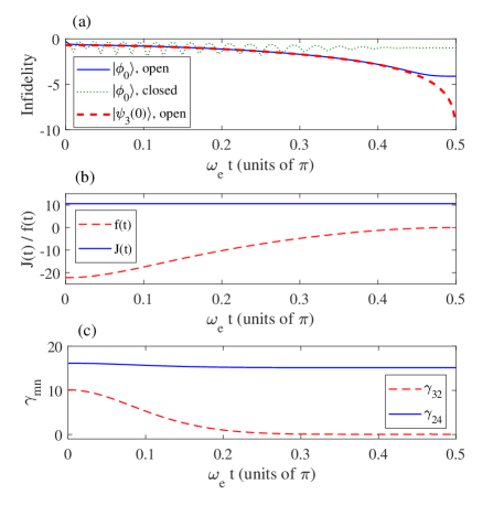
Figure 1: (a) The infidelities between $\rho_{\text{s}}(t)$ and $|\phi_{T}\rangle$ with a perfect initial state $|\psi_{3}(0)\rangle$ (red dashed line) and a preset initial $|\phi(0)\rangle$ for both open (blue solid line) and closed (green dotted line) cases, (b) Transverse field $f(t)$ and the scalar coupling $J(t)$, (c) The decoherence rates $\gamma_{32}$ and $\gamma_{24}$ as functions of the dimensionless time in the unity of $\pi$. The parameters are chosen as $\gamma=1$, $g_{2m}=0.02$, $\delta=\sqrt{0.1}$, $\omega^{c}_{mn}=10\alpha_{mn}$, $s_{24}=0.01$ and $s_{32}=0.1$. We set $\omega_{e}=1$ as a unity of $f(t)$, $J(t)$, $\gamma_{32}$ and $\gamma_{24}$.

For the inverse engineering method, the initial state is not $|\phi_{0}\rangle$, but the initial eigenstate $|\psi_{3}(0)\rangle$. A small amplitude on $|11\rangle$ is required for successful entanglement generation. Even so, because of the decoherence effect, employing a not too large $\delta$, an initial state as $|\phi_{0}\rangle$ can still be transferred to the target state with a satisfied fidelity. This will be shown in the following numerical results.

Next, we show numerical results for the Ohmic coupling spectral density functionBenedetti2018

$$J(\alpha_{mn})=s_{mn}\alpha_{mn}\exp\left(-\frac{\alpha_{mn}}{\omega^{c}_{mn}}\right),$$ (29)

where $s_{mn}$ denotes the dimensionless coupling strength and $\omega^{c}_{mn}$ is the cut-off frequency. In FIG.1 (a), we plot the infidelity $\log_{10}(1-\langle\phi_{T}|\rho_{\text{s}}(t)|\phi_{T}\rangle)$ as a function of dimensionless time $\omega_{e}t$ for a perfectly prepared initial state $|\psi_{3}(0)\rangle$ (the red dashed line) and an imperfect initial state $|\phi_{0}\rangle$ (the blue solid line). As a comparison, we also plot the infidelity for the closed system case, where the evolution of the quantum state governed by Eq(LABEL:eq:meq2) with $\gamma_{mn}=0$. By using the transverse field $f(t)$ and the scalar coupling $J(t)$ as shown in FIG.1 (b), the quantum state transfers into the target entanglement state with a perfect fidelity (the red dashed line in FIG.1 (a)). Obviously, the control protocol given by the inverse engineering method based on the LRIs still works well in open dynamics case. But the differences are also obvious: (i) The inverse engineering does not suit all of eigenstates of the LRI, and only one of them can be used, which corresponds to the instantaneous steady state; (ii) The inverse engineering can be successful only in the zero-temperature reservoir, while it is a mixed state for the finite temperature case (see Eq.(25)).

It should be noticed that, because the instantaneous frequency $\alpha_{mn}$ is time-dependent, the target state may fail to generate, if the ansatz of $g_{i}(t)$ is not chosen well. For instance, if $g_{2m}$ exceeds a particular value (about 0.48 for the parameters chosen in FIG.1), $\alpha_{32}$ will be negative in some time ranges, while $\alpha_{23}$ is becoming positive. Thus the transition direction between $|\psi_{2}(t)\rangle$ and $|\psi_{3}(t)\rangle$ is reversed. In this time range, the Lindblad operators involved in the DMME are $F_{23}(t)$ and $F_{24}(t)$. The instantaneous steady state of the DMME is no longer $|\psi_{3}(t)\rangle$, but $|\psi_{2}(t)\rangle$. Therefore, we will fail to prepare the target state $(|00\rangle-|11\rangle)/\sqrt{2}$. For the parameters used in FIG.1, both $\alpha_{32}$ and $\alpha_{24}$ are still positive which leads to positive decoherence rates as shown in FIG.1(c).

The ansatz given by Eq.(27) provides us with a constant scalar coupling and a decreasing transverse field, which is very similar to the adiabatic engineering protocol. However, the trajectories from the initial state to the target state are different. The adiabatic trajectory is defined by the instantaneous steady state of the adiabatic master equation, i.e, $|\psi_{3}(t)\rangle$ with $\zeta_{2}=0$ (see Eq.(23)). In contrast, $\zeta_{2}(t)$ can be nonzero for the trajectory defined by the instantaneous steady state of the DMME. This is essential for accelerating the adiabatic engineering process. According to Eqs.(18) and (27), $\zeta_{2}(t)$ will be zero if $g_{2m}=0$. Because $J(t),f(t)\propto g_{2m}^{-1}$ (see Eq.(28)), the quantum state can evolve along the adiabatic trajectory by means of either infinite $f$ and $J$, or a infinitesimal $\omega_{e}$. Besides, a proper selection of $g_{2m}$ will reduce the driving strength used in the quantum state engineering.

On the other hand, it is shown by Eq.(28) that the transverse field at $t=0$ satisfies

$$f(0)=\frac{\omega_{e}(g_{1}^{2}(0)+2g_{2m}^{2})}{4g_{2m}g_{6}(0)}.$$

Due to $\delta\rightarrow 0$, it yields $g_{1}(0)\rightarrow\infty$. Thus, if we prepare the initial state on $|00\rangle$, the control protocol requires an infinite transverse field at $t=0$, which leads to the inverse engineering scheme is unavailable. Therefore, we must admit a superposition state of $|00\rangle$ and $|11\rangle$ as the initial state. However, it is difficult to prepare the initial state on $|\psi_{3}(0)\rangle$ precisely. And the starting point of our control mission is not $|\psi_{3}(0)\rangle$, but $|\phi_{0}\rangle=|00\rangle$. Due to the decoherence effect, we can always present a better fidelity than the closed systems case. In FIG.1(a), we plot the evolution of the fidelity for the initial state $|\phi_{0}\rangle$, in which the blue solid line (the green dots line) associates with the mater equation with (without) the dissipator. Since it is unitary evolution for the case without the dissipator, the final fidelity will be 0.9 as shown by the green dotted line in FIG.1(a). In contrast to the closed systems case, the infidelity for the open system case decreases and approaches to a perfect fidelity with the evolution. The decoherence draws the quantum system into $|\psi_{3}(t)\rangle$ gradually. Here, we would like to clarify that the inverse engineering method and the dissipation engineering method are totally different. The inverse engineering method is to transfer the quantum state from an initial eigenstate of the LRI to its final eigenstate, which is usually the target state. But it is true only for the closed quantum systems. For the open quantum system dynamics, the decoherence will draw the quantum state out the eigenstate of the LRI. In contrast, the dissipation engineering method is to generate the target state by means of the decoherence effect. The target state is usually the steady state of open quantum systems. Obviously, our proposal combines the advantages of both two methods, and is robust to errors in initial state preparing. Therefore, the stronger decoherence rates are, the higher fidelity we can obtain within a finite control period.

At last, we would like to emphasise that the ansatz for $g_{i}$ for $i=1,2,6$ will be chosen optionally. For instance, the advantage of the ansatz given in Eq.(27) is that scalar coupling $J$ is constant. Also we can choose

$$g_{1}(t)=g_{1}(0)\sin^{3}\left(\omega_{e}t\right).$$

In this way, the transverse field at $t=0$ reads

$$f(0)=\frac{{g_{2m}}\omega_{e}}{2\,{g_{6}(0)}},$$

which is independent on $g_{1}(0)$. Thus, even $\delta\rightarrow 0$, we can still have a control protocol with a finite transverse field at $t=0$. Meanwhile, the scalar coupling $J$ must be changed with time, which reads

$$J(t)=-\frac{3\,{g_{1}(0)}\omega_{e}}{4\,\pi\,\mathrm{g_{2m}}}\sin\left(\omega_{e}t\right).$$

If $g_{2m}/g_{6}(0)\ll 1$ is set, we will immediately obtain a control protocol starting and ending with zero transverse field.

V Conclusion

In this paper, we explicitly solve the problem of a double two-level system with a time-dependent transverse field and a scalar coupling which interacts with a common heat reservoir in the finite temperature. By means of the driven-Markovian master equation based on the Lewis-Riesenfeld invariants theory, we show that both the decoherence rates and the Lindblad operators are time-dependent, which implies a time-dependent steady state will appear in the open system dynamics. Such a time-dependent steady state is an important candidate in the quantum state engineering of open quantum systems. For instance, if the reservoir is vacuum, the instantaneous steady state is not only a time-dependent pure state, but also one of the LRI’s eigenstates. Therefore, the quantum state can be transferred along the trajectory given by this eigenstate with a perfect fidelity by means of the inverse engineering method for the closed quantum systems, even if the initial state does not prepared precisely. This implies a potential application in the non-adiabatic quantum control by using the inverse engineering method based on the LRIs theoryKang2022 ; Whitty2022 .

As we see, the DMME depends on the driving protocol of the system. The generators of the Hamiltonian in the DMME presented here belongs to a semi-simple subalgebras $so(4)\oplus u(1)$ of the Lie algebras $su(4)$Nakahara2012 . For the other physical models and driving protocols for the double two-level system, we need to analyse symmetry of driving protocol. Based on this symmetry and related semi-simple subalgebras, the LRIs can be obtained explicitly. Fortunately, the LRIs for the driven four-level system have been explored in Ref.Nakahara2012 . Therefore, following the procedure presented in this paper, it is not difficult to derive the DMMEs for different driving protocols.

This work is supported by the National Natural Science Foundation of China (NSFC) under Grants Nos. 12205037, 12075050 .

Appendix A The Lamb shifts Hamiltonian

We start with the DMME in the interaction picture (Eq.(20)). The Lamb shift Hamiltonian is given by Eq.(21). As shown in Sec. IV, there are two Lindblad operators involved in the DMME for the driven double two-level system, i.e., $\tilde{F}_{32}=|\psi_{3}(0)\rangle\langle\psi_{2}(0)|$ and $\tilde{F}_{24}=|\psi_{2}(0)\rangle\langle\psi_{4}(0)|$. Substituting the Lindblad operators into Eq.(21), we immediately obtain the concrete Lamb shift Hamiltonian

$$\tilde{H}_{\text{LS}}= \hbar S(\alpha_{32})\xi_{32}^{2}|\psi_{2}(0)\rangle\langle\psi_{2}(0)|$$

$$+\hbar S(\alpha_{24})\xi_{24}^{2}|\psi_{4}(0)\rangle\langle\psi_{4}(0)|.$$

Since $\alpha_{mn}$ and $\xi_{mn}$ are time-varying, the Lamb shift Hamiltonian in the interaction picture is a time-dependent operator. When the reservoir is at zero temperature, i.e., $N_{mn}=0$, $S(\alpha_{mn})$ can be given analytically. Considering a Ohmic coupling spectral density function as shown in Eq.(29), we have

$$S(\alpha_{mn})=\frac{s_{mn}}{\hbar^{2}}\left[\omega_{c}-\alpha_{mn}\exp\left(-\frac{\alpha_{mn}}{\omega_{c}}\right)\text{Ei}\left(\frac{\alpha_{mn}}{\omega_{c}}\right)\right],$$

where $\text{Ei}(x)=\int_{-\infty}^{x}\ e^{-x^{\prime}}/x^{\prime}dx^{\prime}$ is the one-argument exponential integral function. Thus the Lamb shift Hamiltonian in the Schrödinger picture can be obtained by means of $H_{\text{LS}}=U_{\text{s}}\tilde{H}_{\text{LS}}U_{\text{s}}^{\dagger}$.

In the following, we verify that $|\psi_{3}(t)\rangle$ is the instantaneous steady state, or the dark state, of the DMME with the Lamb shifts. We still focus on the DMME in the interaction picture at first

$$\partial_{t}{\tilde{\rho}}_{\text{s}} \equiv \mathcal{\tilde{L}}\tilde{\rho}_{\text{s}}(t)=-\frac{i}{\hbar}\left[\tilde{H}_{\text{LS}}(t),\tilde{\rho}_{\text{s}}\right]$$ (30)

$$+ \gamma_{32}\left(\tilde{F}_{32}{\tilde{\rho}}_{\text{s}}\tilde{F}_{32}^{\dagger}-\frac{1}{2}\left\{\tilde{F}_{32}^{\dagger}\tilde{F}_{32},{\tilde{\rho}}_{\text{s}}\right\}\right)$$

$$+ \gamma_{24}\left(\tilde{F}_{24}{\tilde{\rho}}_{\text{s}}\tilde{F}_{24}^{\dagger}-\frac{1}{2}\left\{\tilde{F}_{24}^{\dagger}\tilde{F}_{24},{\tilde{\rho}}_{\text{s}}\right\}\right).$$

If the steady state in the interaction picture is $|\psi_{3}(0)\rangle$ , the instantaneous steady of the DMME in the Schrödinger picture must be $|\psi_{3}(t)\rangle$ owing to $\rho_{\text{ss}}(t)=U_{\text{s}}\tilde{\rho}_{\text{ss}}U_{\text{s}}^{\dagger}$. Here we use the criteria of the pure steady state given in Ref.Kraus2008 . It is not difficult to see that $|\psi_{3}(0)\rangle$ satisfies the following conditions, i.e., $\tilde{H}_{\text{LS}}(t)|\psi_{3}(0)\rangle=0$, $\tilde{F}_{32}|\psi_{3}(0)\rangle=0$ and $\tilde{F}_{24}|\psi_{3}(0)\rangle=0$. Therefore, we confirm that $|\psi_{3}(0)\rangle$ is the steady state of the DMME Eq.(30). On the other hand, if we discard the Lamb shifts Hamiltonian, the steady state is not changed, so is the instantaneous steady state in the Schrödinger picture ($|\psi_{3}(t)\rangle$).

In order to show this visibly, we recheck the infidelity between the quantum states, governed by the DMME with and without the Lamb shifts, and the target state $|\Phi_{T}\rangle$, which is shown in FIG.2. When the initial state is chosen as the initial steady state $|\psi_{3}(0)\rangle$, the dynamical evolutions governed by the DMME with and without the Lamb shifts are similar, which is verified by FIG.2 (a). Therefore, we can neglect the Lamb shift terms in the DMME if we are interested in generating a quantum state by the instantaneous steady state. Otherwise, the Lamb shifts may affect the dynamical evolution when we choose the other initial states. In FIG.2 (b), we also plot the infidelity with the initial state $|\psi_{4}(0)\rangle$. As we see, the dynamical evolutions are evidently different at the beginning. With the evolution, they decay into the same steady state $|\psi_{3}(t)\rangle$. Therefore, we can still trust the numerical results in Sec. IV, where there is a tiny population out of the initial steady state.

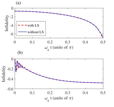
Figure 2: (a) The infidelities between $\rho_{\text{s}}(t)$ and $|\phi_{T}\rangle$ with the Lamb shifts (red dashed line) and without the Lamb shifts (blue solid line) for the initial state $|\psi_{3}(0)\rangle$, (b) The infidelities between $\rho_{\text{s}}(t)$ and $|\phi_{T}\rangle$ with the Lamb shifts (red dashed line) and without the Lamb shifts (blue solid line) for the initial state $|\psi_{4}(0)\rangle$. The parameters are chosen as $\gamma=1$, $g_{2m}=0.02$, $\delta=\sqrt{0.1}$, $\omega^{c}_{mn}=10\alpha_{mn}$, $s_{24}=0.01$ and $s_{32}=0.1$. We set $\omega_{e}=1$ as a unity of $f(t)$, $J(t)$, $\gamma_{32}$ and $\gamma_{24}$.

References

(1) P. Král, I. Thanopulos, and M. Shapiro, Rev. Mod. Phys. 79, 53 (2007).
(2) T. Hatomura, and K. Takahashi, Phys. Rev. A 103, 012220 (2021).
(3) D. Guéry-Odelin, A. Ruschhaupt, A. Kiely, E. Torrontegui, S.
Martínez-Garaot, and J. G. Muga, Rev. Mod. Phys. 91, 045001 (2019).
(4) A. del Campo, and K. Kim, New J. Phys. 21, 050201 (2019).
(5) J. Werschnik, and E. K. U. Gross, J. Phys. B. 40, R175 (2007).
(6) S. C. Hou, M. A. Khan, X. X. Yi, D. Y. Dong, and I. R. Petersen, Phys. Rev. A
86, 022321 (2012).
(7) X. X. Yi, X. L. Huang, C. F. Wu, and C. H. Oh, Phys. Rev. A 80, 052316 (2009).
(8) H. P. Breuer and F. Petruccione, The Theory of Open Quantum Systems
(Oxford University Press, New York, 2007).
(9) E. B. Davies, Commun. Math. Phys. 39, 91 (1974).
(10) E. Davies and H. Spohn, J. Stat. Phys. 19, 511 (1978).
(11) S. Flannigan, F. Damanet, and A. J. Daley, Phys. Rev. Lett. 128, 063601 (2022).
(12) L. Bouten, M. Guta, and H. Maassen, J. Phys. A 37, 3189 (2004).
(13) V. Gorini, A. Kossakowski, and E. C. G. Sudarshan, J. Math. Phys. 17, 821 (1976).
(14) G. Lindblad, Commun. Math. Phys. 48, 119 (1976).
(15) T. Albash, S. Boixo, D. A. Lidar, and P. Zanardi, New J. Phys. 14, 123016 (2012).
(16) A. M. Childs, E. Farhi, and J. Preskill, Phys. Rev. A 65, 012322 (2001).
(17) I. Kamleitner, Phys.Rev.A 87, 042111 (2013).
(18) M. S. Sarandy, L. A. Wu, and D. A. Lidar, Quant. Info. Proc. 3, 331 (2004).
(19) M. Yamaguchi, T. Yuge, and T. Ogawa, Phys. Rev. E 95, 012136 (2017).
(20) R. Dann, A. Levy, and R. Kosloff, Phys. Rev. A 98, 052129 (2018).
(21) P. P. Potts, A. A. Sand Kalaee, and A. Wacker, New J. Phys. 23, 123013 (2021).
(22) R. Dann, A. Tobalina, and R. Kosloff, Phys. Rev. A 101, 052102 (2020).
(23) H. R. Lewis Jr., J. Math. Phys. 9, 1976 (1968).
(24) H. R. Lewis Jr. and W. B. Riesenfeld, J. Math. Phys. 10, 1458 (1969).
(25) S. L. Wu, X. L. Huang, and X. X. Yi, Phys. Rev. A 106, 052217 (2022).
(26) R. I. Karasik, K. P. Marzlin, B. C. Sanders, and K. B. Whaley, Phys. Rev. A 77, 052301 (2008).
(27) S. L. Wu, X. L. Huang , H. Li , and X. X. Yi, Phys. Rev. A 96, 042104 (2017).
(28) X. Chen, A. Ruschhaupt, S. Schmidt, A. del Campo, D. Guéry-Odelin, and J. G. Muga,
Phys. Rev. Lett. 104, 063002 (2010).
(29) X. Chen, and J. G. Muga, Phys. Rev. A, 82, 053403 (2010).
(30) M. Herrera, M. S. Sarandy, E. I. Duzzioni, and R. M. Serra, Phys. Rev. A 89, 022323 (2014).
(31) J. Jing, L. A. Wu, M. S. Sarandy, and J. G. Muga, Phys. Rev. A 88, 053422 (2013).
(32) A. G. Redfield, Advances in Magnetic and Optical Resonance (Elsevier, 1965).
(33) T. Petrosky and I. Prigogine, The Liouville Space Extension of Quantum Mechanics,
edited by I. Prigogine and S. A. Rice (John Wiley & Sons, New York, 1997).
(34) I. S. Oliveira, R. S. Sarthour Jr, T. J. Bonagamba, J. C. C. Freitas, andE. R. deAzevedo,
NMR Quantum Information Processing (Elsevier, Amsterdam, 2007).
(35) J. Maziero, R. Auccaise, L. C. Céleri, D. O. Soares-Pinto, E. R. deAzevedo, T. J. Bonagamba,
R. S. Sarthour, I. S. Oliveira, and R. M. Serra, Braz. J. Phys. 42, 86 (2013).
(36) D. Farina, V. Giovannetti, Phys. Rev. A 100, 012107 (2019).
(37) M. Cattaneo, G. L. Giorgi, S. Maniscalco, and R. Zambrini,
Phys. Rev. A 101, 042108 (2020).
(38) B. Kraus, H. P. Büchler, S. Diehl, A. Kantian, A. Micheli, and P. Zoller, Phys. Rev. A 78, 042307 (2008).
(39) M. S. Sarandy and D. A. Lidar, Phys.Rev.A 71, 012331 (2005).
(40) L. C. Venuti, T. Albash, D. A. Lidar, and P. Zanardi, Phys. Rev. A. 93, 032118 (2016).
(41) J. B. Altepeter, P. G. Hadley, S. M. Wendelken, A. J. Berglund, and P. G. Kwiat,
Phys. Rev. Lett. 92, 147901 (2004).
(42) W. Qin, C. Wang, and X. Zhang, Phys. Rev. A 91, 042303 (2015).
(43) A. C. Santos, and M. S. Sarandy, Phys. Rev. A 104, 062421 (2021).
(44) C. Benedetti, F. Salari Sehdaran, M. H. Zandi, and M. G. A. Paris, Phys. Rev. A 97, 012126 (2018).
(45) Y. H. Kang, Y. H. Chen, X. Wang, J. Song, Y. Xia, A. Miranowicz, S. B. Zheng, and F. Nori,
Phys. Rev. Research 4, 013233 (2022).
(46) C. Whitty, A. Kiely, and A. Ruschhaupt, Phys. Rev. A 105, 013311 (2022).
(47) U. Güngördü, Y. Wan, M. A. Fasihi, and M. Nakahara, Phys. Rev. A 86, 062312 (2012).