Non-Hermitian Quantum Fermi Accelerator

Abstract:

We exactly solve a quantum Fermi accelerator model consisting of a time-independent non-Hermitian Hamiltonian with time-dependent Dirichlet boundary conditions. A Hilbert space for such systems can be defined in two equivalent ways, either by first constructing a time-independent Dyson map and subsequently unitarily mapping to fixed boundary conditions or by first unitarily mapping to fixed boundary conditions followed by the construction of a time-dependent Dyson map. In turn this allows to construct time-dependent metric operators from a time-independent metric and two time-dependent unitary maps that freeze the moving boundaries. From the time-dependent energy spectrum, we find the known possibility of oscillatory behavior in the average energy in the PT-regime, whereas in the spontaneously broken PT-regime we observe the new feature of a one-time depletion of the energy. We show that the PT broken regime is mended with moving boundary, equivalently to mending it with a time-dependent Dyson map.

1 Introduction

Classical versions of Fermi accelerators were originally proposed by Fermi [1] more than seventy years ago as a possible explanation for the high energies observed in cosmic radiation. The simplest classical Fermi accelerator model consists of a free particle moving between two walls simulating magnetic fields, with one of them fixed and the other moving in time, with the collisions between the particle and the walls being perfectly elastic. Besides predicting features of cosmic rays in the spirit of the original motivation, such as the maximum energy that particles can reach is proportional to the strength of the magnetic field and the size of the acceleration region, the models were also found to exhibit classical chaotic behavior [2, 3, 4]. The latter is due to the fact that the description in phase-space of consecutive scatterings between the walls and the particle leads to nonlinear maps, which in their simplest version, corresponding to the so-called Ulam maps. For a recent overview of the latest experimental observations of ultra-high energy cosmic rays, see for instance [5].

Quantum versions of Fermi accelerator models are set up in a similar fashion, described by the Schrödinger equation with Dirichlet boundary conditions. They allow us to study quantum chaos [6, 7] and other interesting phenomena [8, 9, 10, 11, 12, 13], such as the possibility of an energy gain in the time-dependent spectrum. Here the purpose is to investigate such a system with the starting Hamiltonian taken to be non-Hermitian, but $\mathcal{PT}$-symmetric/pseudo-Hermitian. In the broken $\mathcal{PT}$-regime we observe the new feature of declaration.

Our starting point is to consider a time-independent $\mathcal{PT}$-symmetric/pseudo-Hermitian [14, 15] Hamiltonian $\tilde{H}=-\frac{\hbar^{2}}{2m}\partial_{x}^{2}+\tilde{V}(x)$, where $\tilde{V}(x)$ is a non-Hermitian potential. The Schrödinger equation with Dirichlet boundary condition is given by

$$i\hbar\frac{\partial}{\partial t}\tilde{\psi}(t,x)=\tilde{H}(x)\tilde{\psi}(t,x),\qquad\tilde{\psi}(t,\pm\ell)=0,$$ (1)

where $\ell>0$. The Hilbert space of the system consists of square-integrable functions in the interval $[-\ell,\ell]$, i.e., $\tilde{\psi}(t,x)\in L^{2}([-\ell,\ell])$. This Hamiltonian is said to be $\mathcal{PT}$-symmetric if the Hamiltonian and the wave functions are symmetric under an anti-linear transformation, such as $p\rightarrow p$, $x\rightarrow-x$, and $i\rightarrow-i$, in our case.

The standard procedure in $\mathcal{PT}$-symmetric quantum mechanics is to map the non-Hermitian Hamiltonian (1) to a Hermitian Hamiltonian with a Dyson map $\eta$ such that $\tilde{H}=\eta\tilde{h}\tilde{\eta}^{-1}\not=\tilde{H}^{\dagger}$, $\tilde{h}^{\dagger}=\tilde{h}$. Let us denote the new wave function $\tilde{\phi}(t,x)=\tilde{\eta}\tilde{\psi}(t,x)$ where the non-Hermitian operator $\tilde{\eta}$ is time-independent. Therefore the Schrödinger equation and the boundary condition (1) are simply mapped to

$$i\hbar\frac{d}{dt}\tilde{\phi}(t,x)=\tilde{h}(x)\tilde{\phi}(t,x),\qquad\tilde{\phi}(t,\pm\ell)=0.$$ (2)

In $\mathcal{PT}$-symmetric quantum mechanics inner product in the Hilbert space needs to be redefined. Accordingly, the average energy of the non-Hermitian Hamiltonian is given by $\braket{E}_{\eta}\equiv\int_{-\ell}^{\ell}dx\tilde{\psi}\tilde{\rho}\tilde{H}\tilde{\psi}$, where the Hermitian positive definite metric is defined as $\tilde{\rho}:=\tilde{\eta}^{\dagger}\tilde{\eta}$. This can be rewritten in terms of the Hermitian Hamiltonian as

$$\braket{E(t)}_{\eta}:=\int_{-\ell}^{\ell}dx\tilde{\psi}\tilde{\rho}\tilde{H}\tilde{\psi}=\int_{-\ell}^{\ell}dx\tilde{\phi}\tilde{h}\tilde{\phi}.$$ (3)

The common characteristic of the non-Hermitian system is that the above equality only holds when the non-Hermitian Hamiltonian and the wave function are $\mathcal{PT}$-symmetric. The average energy of $\tilde{H}$ acquires complex conjugate eigenvalues in the $\mathcal{PT}$-broken regime.

It has been established that real-valued average energies can be obtained in all regimes when the non-Hermitian Hamiltonian or the Dyson map are time-dependent [16]. In this work, we demonstrate that real-valued average energies can also be attained in the $\mathcal{PT}$-broken regime of the Swanson model by introducing time-dependence to the boundary condition $\ell$, instead of the Hamiltonian or Dyson map. Moreover, we establish the equivalence of our approach with a previous method [16], where the Dyson map’s time-dependence was used to mend the $\mathcal{PT}$-broken regime. Our two primary findings are summarized in Table 1 and Fig. 1. We will provide the explicit derivation of the scheme in Fig. 1 in the next section.

	$\mathcal{PT}$-symmetric	$\mathcal{PT}$-broken
Time-independent boundary condition	$\braket{E}_{\eta}\in\mathbb{R}$	$\braket{E}_{\eta}\in\mathbb{C}$
Time-dependent boundary condition	$\braket{E}_{\eta}\in\mathbb{R}$	$\braket{E}_{\eta}\in\mathbb{R}$

Table 1: The average energy $\braket{E}_{\eta}$ defined in Eq. (3) is compared for two $\mathcal{PT}$-regimes with time-dependent/independent boundary conditions. In both cases there is a phase transition in the dynamical behavior of $\braket{E}_{\eta}$ between $\mathcal{PT}$ broken/unbroken regimes. The detail is presented in section 3.

2 Equivalence of time-dependent boundary and Dyson map

Let us assume that the boundary is time-dependent, i.e., $\ell=\ell(t)$, then, the wave functions $\tilde{\psi}(t,x)$ and $\tilde{\psi}(t^{\prime},x)$ belong to two different Hilbert spaces for $t\not=t^{\prime}$. Therefore, the time derivative of the wave function does not belong to any Hilbert space for any time slice, which implies that the above Schrödinger equation is not well-defined. However, in [17], the problem was resolved by formally embedding the system into a larger domain $L^{2}(\mathbb{R})=L^{2}([-\ell,\ell])\oplus L^{2}((-\infty,-\ell)\cup(\ell,\infty))$, where extended Hamiltonian is $\tilde{H}(x)\oplus 0$. This embedding implies that the integration contour of the average energy (3) can be understood as

$$\braket{E(t)}_{\eta}=\int_{-\infty}^{\infty}dx\tilde{\psi}\tilde{\rho}\left[\tilde{H}(x)\oplus 0\right]\tilde{\psi}=\int_{-\ell(t)}^{\ell(t)}dx\tilde{\psi}\tilde{\rho}\left[\tilde{H}(x)\right]\tilde{\psi}.$$ (4)

To remove the time dependence of the boundary from the Hilbert space, a time-dependent unitary operator $U(t)$ is introduced as

$$\begin{array}[]{cccc}U:&L^{2}(\mathbb{R})&\rightarrow&L^{2}(\mathbb{R})\\ &f(t,x)&\rightarrow&\quad\sqrt{\ell(t)}f\left(t,\ell(t)x\right),\end{array}$$ (5)

which maps all wave functions in $L^{2}(\mathbb{R})$ to $L^{2}(\mathbb{R})=L^{2}([-1,1])\oplus L^{2}((-\infty,-1)\cup(1,\infty))$, thereby removing the time dependence of the boundary from the Hilbert space. The factor $\sqrt{l(t)}$ is necessary to ensure the transformation is unitary. The Hamiltonian is mapped to $U\tilde{H}U^{\dagger}\oplus 0$. For the rest of the paper, we will drop the $0$ component of the extended operators for brevity.

Let us define the unitary transformed wave function as $U(t)\tilde{\psi}(t,x)\equiv\psi(t,x)$. The time-dependent Schrödinger equation (1) is also mapped by the unitary operator as

$$i\hbar\frac{\partial}{\partial t}\psi(t,y) = \left(U\tilde{H}(x)U^{\dagger}+i\hbar U\partial_{t}U^{\dagger}\right)\psi(t,y)$$ (6)

$$= \left[\tilde{H}(y)+\frac{\partial_{t}\ell}{2\ell}\left\{y,i\hbar\partial_{y}\right\}\right]\psi(t,y)\equiv H(t,y)\psi(t,y)$$

where $y=\ell x\in[-1,1]$.

Alternatively, assuming pseudo-Hermiticity, the time-independent non-Hermitian Hamiltonian (1) can be mapped to a Hermitian Hamiltonian via Dyson map $\tilde{H}=\eta\tilde{h}\tilde{\eta}^{-1}$, $\tilde{h}^{\dagger}=\tilde{h}$. In this case, let us denote the new wave function $\tilde{\phi}(t,x)=\tilde{\eta}\tilde{\psi}(t,x)$ where the non-Hermitian operator $\tilde{\eta}$ is time-independent. Therefore the Schrödinger equation and the boundary condition (1) are simply mapped to

$$i\hbar\frac{d}{dt}\tilde{\phi}(t,x)=\tilde{h}(x)\tilde{\phi}(t,x),\qquad\tilde{\phi}(t,\pm\ell)=0.$$ (7)

Then the above procedure to remove the boundary time dependence can be applied to the mapped Hermitian system, and one obtains

$$i\hbar\frac{d}{dt}\phi(t,y) = \left(u\tilde{h}u^{\dagger}-i\hbar u\partial_{t}u^{\dagger}\right)\phi(t,y)$$ (8)

$$= \left[\tilde{h}(y)+\frac{\partial_{t}\ell}{2\ell}\left\{y,i\hbar\partial_{y}\right\}\right]\phi(t,y)\equiv h(t)\phi(t,y),$$ (9)

where $u\tilde{\phi}(t,x)\equiv\phi(t,y)$ and $u$ is also defined in a same way as Eq. (5).

It has been shown that in the time-dependent case, the Dyson map between non-Hermitian and Hermitian operators is given by

$$H(t)=\eta(t)h(t)\eta(t)^{-1}+i\hbar\frac{\partial\eta}{\partial t}\eta^{-1},$$ (10)

where the Dyson map $\eta(t)$ is a time-dependent non-Hermitian operator. We summarise the relation between Eqs.(1), (6), (7) and (9) in the Fig. 1. Note that by requiring the scheme in Fig. 1 to be commutative, we find the relation between two similarity transformations and the two Dyson maps

$$\eta(t)=u(t)\tilde{\eta}U^{\dagger}(t),$$ (11)

which leads to the equivalence between the non-Hermitian time-dependent boundary problem (1) and the non-Hermitian time-dependent Hamiltonian problem with a time-dependent metric (6) discussed in [16].

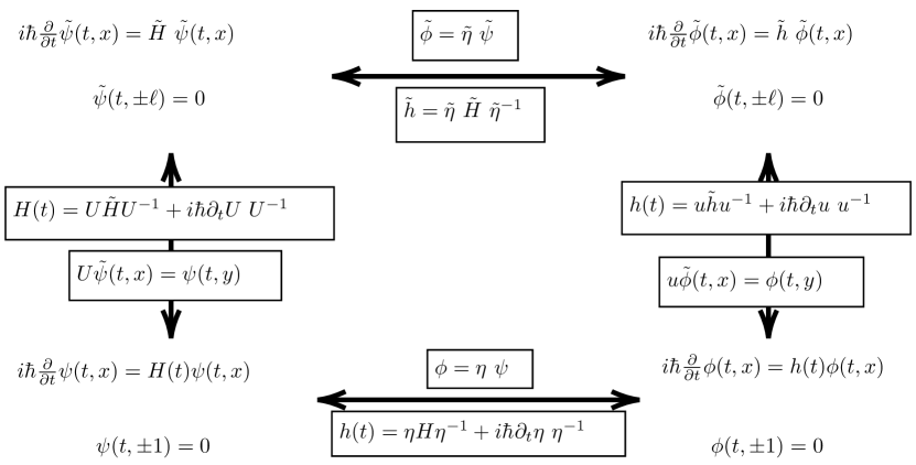
Figure 1: Commutative scheme, showing the relations between two time-independent Schrödinger equations with time-dependent boundary conditions on the top row, and two time-dependent Schrödinger equations with time-independent boundary conditions on the bottom row.

Once we obtain the time-dependent Hermitian Hamiltonian, the average energy (3) can be calculated. Using the relations in Fig. 1 and the Eq. (11), one can write down four alternative formulations of the average energy (3).

$$\braket{E(t)} = \int_{-\ell(t)}^{\ell(t)}dx\tilde{\psi}^{\dagger}\tilde{\rho}\tilde{H}\tilde{\psi}=\int_{-\ell(t)}^{\ell(t)}dx\tilde{\phi}^{\dagger}\tilde{h}\tilde{\phi}$$ (12)

$$= \int_{-1}^{1}dx\phi^{\dagger}\left(h-i\hbar u_{t}u^{\dagger}\right)\phi$$ (13)

$$= \int_{-1}^{1}dx\psi^{\dagger}\eta^{\dagger}\eta\left[H+i\hbar\left(u^{\dagger}\eta\right)^{-1}\partial_{t}\left(u^{\dagger}\eta\right)\right]\psi.$$ (14)

We will apply these relations to the Swanson model in the next section.

3 Swanson model: Mending $\mathcal{PT}$-broken regime via moving boundary

To see how a time-dependent boundary can lead to real average energy in both $\mathcal{PT}$-symmetric and broken regimes, let us consider the Swanson Hamiltonian [18]

$$\tilde{H}=\frac{\omega_{-}}{2}p^{2}+\frac{\omega_{+}}{2}x^{2}+\frac{i}{2}\mathcal{A}\{x,p\},\quad i\hbar\partial_{t}\tilde{\psi}=\tilde{H}\tilde{\psi},$$ (15)

where $p=-i\hbar\partial_{x}$, $\omega_{\pm}:=\omega\pm(\alpha+\beta)$ and $\mathcal{A}:=\alpha-\beta$. According to [19], the Hamiltonian (15) can be mapped via a similarity transformation to a harmonic oscillator, which corresponds to the top-right corner of the commutative diagram in Fig. 1

$$\tilde{\eta}_{i}\tilde{H}\tilde{\eta}^{-1}_{i}=A_{i}(\alpha,\beta)p^{2}+B_{i}(\alpha,\beta)x^{2}\equiv\tilde{h}_{i},\quad\tilde{\eta}_{i}\tilde{\psi}=\tilde{\phi}_{i},\quad i\hbar\partial_{t}\tilde{\phi}_{i}=\tilde{h}_{i}\tilde{\phi}_{i},$$ (16)

where the index $i$ labels the non-unique choices of the Dyson maps. The specific forms of the parameters $A_{i}(\omega,\alpha,\beta)$ and $B_{i}(\omega,\alpha,\beta)$ are fixed by assuming at least two operators to be mapped to their Hermitian counterparts [20]. Below we list three examples taken from [19]

$$A_{1} = \frac{\omega-2\sqrt{\alpha\beta}}{2\omega},\quad B_{1}=\frac{\omega\left(\omega+2\sqrt{\alpha\beta}\right)}{2}:\tilde{\eta}_{i}H\tilde{\eta}_{i}^{-1}=\tilde{h}_{i},\quad\tilde{\eta}_{i}N\tilde{\eta}^{-1}_{i}=N,$$ (17)

$$A_{2} = \frac{\omega-\alpha-\beta}{2\omega},\quad B_{2}=\frac{\omega}{2}\frac{\omega^{2}-4\alpha\beta}{\omega-\alpha-\beta}:\tilde{\eta}_{i}H\tilde{\eta}_{i}^{-1}=\tilde{h}_{i},\quad\tilde{\eta}_{i}x\tilde{\eta}_{i}^{-1}=x,$$ (18)

$$A_{3} = \frac{\omega^{2}-4\alpha\beta}{2\omega\left(\omega+\alpha+\beta\right)},\quad B_{3}=\frac{\omega\left(\omega+\alpha+\beta\right)}{2}:\tilde{\eta}_{i}H\tilde{\eta}_{i}^{-1}=\tilde{h}_{i},\quad\tilde{\eta}_{i}p\tilde{\eta}^{-1}_{i}=p,$$ (19)

where $N$ is a number operator.

The average energy (3) of the Hamiltonian is computed to

$$\braket{E}=(n+1/2)\sqrt{\omega^{2}-4\alpha\beta}=(n+1/2)\sqrt{\mathcal{A}^{2}+\omega_{+}\omega_{-}}$$ (20)

for $n\in\mathbb{N}$. The $\mathcal{PT}$ symmetry of the Swanson model is broken when $\omega^{2}-4\alpha\beta=\mathcal{A}^{2}+\omega_{+}\omega_{-}<0$. Therefore in the $\mathcal{PT}$-broken regime, the average energy becomes complex. This is a common feature of $\mathcal{PT}$-symmetry quantum mechanics. We will consider the time-dependent boundary to mend this complex energy analog to [16].

The Schrödinger equation (16) can be transformed by the unitary map (5) to give the time-dependent Hermitian Schrödinger equation $i\hbar\partial_{t}\phi_{i}=h\phi_{i}$ corresponding to the bottom right corner of the commutative diagram in Fig. 1. The explicit form of the time-dependent Hermitian Hamiltonian is

$$h_{i}(t,x)\equiv\frac{\ell_{t}}{2\ell}\left\{x,i\hbar\partial_{x}\right\}-\frac{\hbar^{2}A_{i}}{\ell^{2}}\partial_{x}^{2}+B_{i}\ell^{2}x^{2}.$$ (21)

for $i=1,2,3$. The corresponding Schrödinger equation is simplified by performing a further unitary transformation of the form $\phi_{j}=c_{1}\text{exp}\left({i\frac{\ell\ell_{t}}{4A_{j}\hbar}x^{2}}\right)\varphi_{j}(t,x)$, which reduces the equation to

$$i4\hbar A_{j}\ell^{2}(\varphi_{j})_{t}+\hbar^{2}4A_{j}^{2}(\varphi_{j})_{yy}-\ell^{3}(4A_{j}B_{j}\ell+\ell_{tt})y^{2}\varphi_{j}=0,$$ (22)

with $c_{j}$ denoting the normalization constant. It is useful to notice that the combination of two parameters $4A_{j}B_{j}=\omega^{2}-4\alpha\beta\equiv\Omega$ takes the same form for all three examples (17) - (19).

The above equation can be reduced further into the effective Harmonic oscillator if we consider the solution to the equation $\ell^{3}(\Omega\ell+\ell_{tt})=\kappa^{2}$ where $\kappa$ is some constant. This is an Ermakov-Pinney equation [21, 22], which can be solved exactly. One of the solutions is

$$\ell^{2}_{j}(t) = \frac{\kappa}{A_{j}B_{j}}\sin^{2}\left(2\sqrt{A_{j}B_{j}}t\right)+\kappa\cos^{2}\left(2\sqrt{A_{j}B_{j}}t\right)$$ (23)

$$+2\kappa\sqrt{\frac{1}{A_{j}B_{j}}-\frac{1}{4A_{j}B_{j}}}\sin\left(2\sqrt{A_{j}B_{j}}t\right)\cos\left(2\sqrt{A_{j}B_{j}}t\right).$$

Introducing the new time variable $\tau=\int^{t}1/\ell^{2}$, we find the effective Harmonic oscillator

$$i4\hbar A_{j}(\varphi_{j})_{\tau}+\hbar^{2}4A^{2}_{j}(\varphi_{j})_{yy}-\kappa^{2}y^{2}\varphi_{j}=0.$$ (24)

Let us consider the Ansatz $\varphi_{j}^{n}=\exp\left(-i\epsilon^{n}_{j}\tau_{j}/A_{j}\hbar\right)\chi_{j}^{n}(y)$. Then the above effective harmonic oscillator is reduced to a Sturm-Liouville eigenvalue problem

$$-\partial_{yy}\chi_{j}^{n}+\frac{\kappa^{2}}{4\hbar^{2}A_{j}^{2}}y^{2}\chi_{j}^{n}=\epsilon_{j}^{n}\chi_{j}^{n}.$$ (25)

where there exist odd and even solutions are given in terms of hypergeometric functions

$${\chi_{\text{odd}}}_{j}^{n}(y) = e^{-\frac{1}{2}\frac{\kappa y^{2}}{2\hbar A_{j}}}\left(\frac{\sqrt{\kappa}y}{\sqrt{2\hbar A_{j}}}\right){{}_{1}}F_{1}\left[\frac{3}{4}-\frac{1}{4}\frac{2\hbar A_{j}}{\kappa}\epsilon_{j}^{n},\frac{3}{2},\frac{\kappa y^{2}}{2\hbar A_{j}}\right],$$ (26)

$${\chi_{\text{even}}}_{j}^{n}(y) = e^{\frac{1}{2}\frac{\kappa y^{2}}{2\hbar A_{j}}}{{}_{1}}F_{1}\left[\frac{1}{4}+\frac{1}{4}\frac{2\hbar A_{j}}{\kappa}\epsilon_{j}^{n},\frac{1}{2},\frac{-\kappa y^{2}}{2\hbar A_{j}}\right].$$ (27)

Therefore we found the solution to the effective Schrödinger equation corresponding to the bottom right corner of the commutative diagram shown in Fig. 1

$$\phi_{j}^{n}(t,x)=c^{j}_{n}e^{i\frac{\ell\ell_{t}}{4A_{j}\hbar}x^{2}-i\frac{1}{A_{j}\hbar}\epsilon_{j}^{n}\tau_{j}}\chi_{j}^{n}(x).$$ (28)

where the constants $c_{n}^{j}$ are fixed by normalisation $1=\braket{\phi_{j}^{n}}{\phi_{j}^{n}}\implies c_{n}^{-2}=\int_{-1}^{1}dy\chi_{n}^{\dagger}\chi_{n}$.

The solution (28) can be mapped back to $\tilde{\phi}$ by use of an inverse mapping with the unitary transformation $u^{\dagger}\phi(t,x)=\phi(t,x/\ell(t))/\sqrt{\ell(t)}$, which gives

$$\tilde{\phi}_{j}^{n}(t,x)=\frac{c_{n}^{j}}{\sqrt{\ell(t)}}e^{i\frac{\ell\ell_{t}}{4A_{j}\hbar}\left(\frac{x}{\ell(t)}\right)^{2}-i\frac{1}{A_{j}\hbar}\epsilon_{j}^{n}\tau_{j}}\chi_{j}^{n}\left(x/\ell(t)\right).$$ (29)

Using this solution together with the Hamiltonian (16), one can calculate the average energy (12).

3.1 Average energy

Next, let us plot the average energy (12) for three different Dyson maps (17) - (19) in the $\mathcal{PT}$-symmetric ($\Omega>0$) and the $\mathcal{PT}$-broken ($\Omega<0$) regimes.

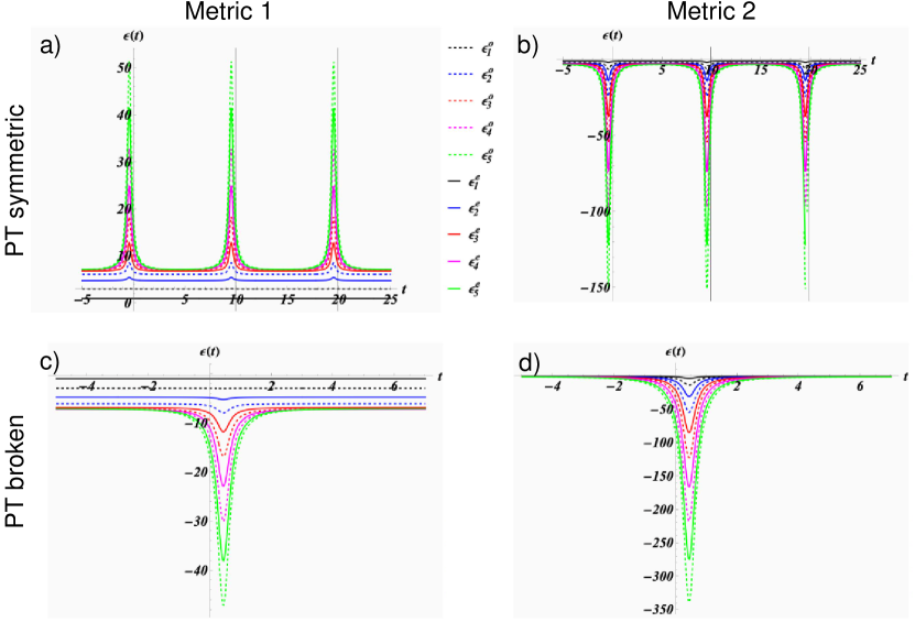
Figure 2: Average energy for the $\mathcal{PT}$-symmetric/broken regimes over time for the first metric (17) in panels (a) and (c), respectively. The results computed with the second metric (18) for $\mathcal{PT}$-symmetric/broken regimes are shown in panels (b) and (d), respectively. The case involving the third metric (19) is omitted as it is almost identical to the first metric with a slight scale difference.

In the $\mathcal{PT}$-symmetric regime shown in Fig. 2 panel (a) and (b), the average energy exhibits the periodic structure with $T=n\pi/2\sqrt{A_{j}B_{j}}$, $n\in\mathbb{Z}$ for all three metrics (17)-(19). This is because the average energy’s periodicity is inherited from the boundary function (23), where the combination $A_{i}B_{i}$ is equal for all metrics. This finding leads us to the same conclusion as in [23], indicating that although the energy expectation value experiences time-dependent fluctuations, it remains periodic with no net gain or loss over a long time.

In the $\mathcal{PT}$-broken regime, the real-valued average energy is consistent with previous observations [16]. As shown in Figs. 2 (c) and (d), the average energy loses its periodic structure in this regime due to the non-periodic behavior of the boundary function (23), which hyperbolically diverges with time. Despite the divergent nature of the boundary function, the average energy remains constant over time and only experiences gain and loss near the origin. This is due to the spreading probability density, which compensates for the divergence of the boundary function, as illustrated in Fig. 3. This behavior is similar to that observed in single-particle open quantum systems [24], but it differs from the context considered here in time-dependent pseudo-Hermitian non-Hermitian systems, where the non-Hermitian term does not result from environmental effects, as in [24].

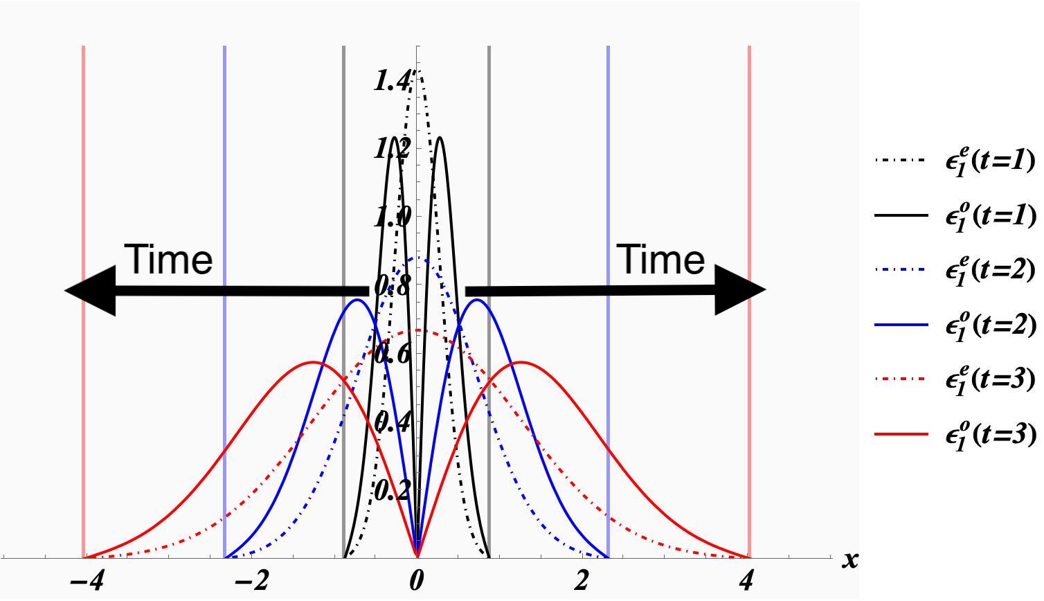
Figure 3: Showing the infinite spreading of the probability density $\tilde{\phi}^{\dagger}\tilde{\phi}$ of the wave function (29) with time in $\mathcal{PT}$-broken regime. The vertical line is the boundary $\ell(t)$, which is found by solving the Ermakov-Pinney equation. In the $\mathcal{PT}$-symmetric regime, the boundary moves periodically with a similar spreading of the probability density.

4 Swanson model: Equivalence of time-dependent boundary and Dyson map

This section illustrates the commutativity of the diagram shown in Fig. 1.

Let us begin with the Swanson model (15). Performing the unitary transformation (5), the time-dependent non-Hermitian Hamiltonian is given in (6), where its explicit form is found to

$$i\hbar\partial_{t}\psi=-\frac{\omega_{-}\hbar^{2}}{2\ell^{2}}\psi_{yy}+\frac{\omega_{+}\ell^{2}}{2}y^{2}\psi+{\hbar\mathcal{A}y\psi_{y}}+\frac{\hbar\mathcal{A}}{2}\psi+\frac{\ell_{t}}{2\ell}\left\{y,i\hbar\partial_{x}\right\}\psi$$ (30)

Similar to the previous section, one can perform further unitary transformations by $\psi=\exp(i\ell\partial_{t}\ell/2\hbar\omega_{-}y^{2})\varphi(t,y)$ to the above equation. Let us consider the following Dyson map

$$\eta=e^{-\frac{1}{2\hbar\omega_{-}}\mathcal{A}\ell^{2}y^{2}},\quad\eta\psi=\eta e^{\frac{1}{2\hbar\omega_{-}}iLL_{t}y^{2}}\psi(t,y)=e^{\frac{1}{2\hbar\omega_{-}}\left(-\mathcal{A}L^{2}+iLL_{t}\right)y^{2}}\varphi(t,y),$$ (31)

which maps the non-Hermitian Hamiltonian to Hermitian Hamiltonian

$$i2\hbar\omega_{-}\ell^{2}\varphi_{t}+\hbar^{2}\omega_{-}^{2}\phi_{yy}-\ell^{3}\left(\Omega\ell+\ell_{tt}\right)y^{2}\phi=0.$$ (32)

Rescaling the variable as $y=\sqrt{\omega_{-}/2A_{i}}z$, the above equation is mapped to the effective Hamiltonian (22), rendering the equivalence of two approaches.

5 Conclusion

Our main finding is that time-dependent boundary conditions can be simulated with time-dependent metric operators and vice versa. In turn, this implies that the spontaneously broken $\mathcal{PT}$ regime can be mended, in the sense of acquiring real energies, not only by a time-dependent metric but equivalently also with time-dependent boundaries. We demonstrated our assertions for the exactly solvable pseudo-Hermitian Swanson model. For this model, the time-dependent boundary functions are restricted by the Ermakov-Pinney equation. The characteristic behavior of this function, which is periodic in time or divergent, is inherited by the time-dependent average of the energy function. These restrictions may be relaxed at the cost of the model no longer exactly solvable.

In the $\mathcal{PT}$-symmetric regime, we find an oscillatory behavior of the average energy similar to the one found in [11] for the harmonic oscillator with time-dependent coefficients. Different types of metric operators distinguish between whether this function has well-localized minima or maxima. In the spontaneously broken $\mathcal{PT}$-regime, the average energy is no longer periodic and develops only one well-localized minimum, irrespective of the choice of the metric.

References

- [1] E. Fermi, On the origin of the cosmic radiation, Phys. Rev. 75(8), 1169 (1949).
- [2] S. Ulam, On some statistical properties of dynamical systems, in Proceedings of the 4th Berkeley Symposium on Mathematical Statistics and Probability, volume 3, pages 315–320, University of California Press, 1961.
- [3] G. Zaslavskii and B. V. Chirikov, Stochastic instability of non-linear oscillations, Soviet Physics Uspekhi 14(5), 549 (1972).
- [4] A. Lichtenberg, M. Lieberman, and R. Cohen, Fermi acceleration revisited, Physica D: Nonlinear Phenomena 1(3), 291–305 (1980).
- [5] D. Gora and P. A. Collaboration, The Pierre Auger Observatory: review of latest results and perspectives, Universe 4(11), 128 (2018).
- [6] G. Karner, On the quantum Fermi accelerator and its relevance to ‘quantum chaos’, letters in mathematical physics 17, 329–339 (1989).
- [7] P. Seba, Quantum chaos in the Fermi-accelerator model, Physical Review A 41(5), 2306 (1990).
- [8] S. Doescher and M. Rice, Infinite square-well potential with a moving wall, American Journal of Physics 37(12), 1246–1249 (1969).
- [9] A. Munier, J. Burgan, M. Feix, and E. Fijalkow, Schrödinger equation with time-dependent boundary conditions, Journal of Mathematical Physics 22(6), 1219–1223 (1981).
- [10] D. Pinder, The contracting square quantum well, American Journal of Physics 58(1), 54–58 (1990).
- [11] A. Makowski and S. Dembiński, Exactly solvable models with time-dependent boundary conditions, Physics Letters A 154(5-6), 217–220 (1991).
- [12] P. Pereshogin and P. Pronin, Geometrical treatment of nonholonomic phase in quantum mechanics and applications, International journal of theoretical physics 32, 219–236 (1993).
- [13] V. Dodonov, A. Klimov, and D. Nikonov, Quantum particle in a box with moving walls, Journal of mathematical physics 34(8), 3391–3404 (1993).
- [14] C. M. Bender and S. Boettcher, Real spectra in non-Hermitian Hamiltonians having P T symmetry, Physical review letters 80(24), 5243 (1998).
- [15] A. Mostafazadeh, Pseudo-Hermiticity versus PT symmetry: the necessary condition for the reality of the spectrum of a non-Hermitian Hamiltonian, Journal of Mathematical Physics 43(1), 205–214 (2002).
- [16] A. Fring and T. Frith, Mending the broken PT-regime via an explicit time-dependent Dyson map, Physics Letters A 381(29), 2318–2323 (2017).
- [17] S. Di Martino, F. Anza, P. Facchi, A. Kossakowski, G. Marmo, A. Messina, B. Militello, and S. Pascazio, A quantum particle in a box with moving walls, Journal of Physics A: Mathematical and Theoretical 46(36), 365301 (2013).
- [18] M. S. Swanson, Transition elements for a non-Hermitian quadratic Hamiltonian, Journal of Mathematical Physics 45(2), 585–601 (2004).
- [19] D. Musumbu, H. Geyer, and W. Heiss, Choice of a metric for the non-Hermitian oscillator, Journal of Physics A: Mathematical and Theoretical 40(2), F75 (2006).
- [20] F. Scholtz, H. Geyer, and F. Hahne, Quasi-Hermitian operators in quantum mechanics and the variational principle, Annals of Physics 213(1), 74–101 (1992).
- [21] E. Pinney, The nonlinear differential equation y+ p (x) y+ cy- 3= 0, in Proc. Amer. Math. Soc, volume 1, pages 681–681, 1950.
- [22] V. P. Ermakov, Second-order differential equations: conditions of complete integrability, Applicable Analysis and Discrete Mathematics , 123–145 (2008).
- [23] A. Makowski and S. Dembiński, Exactly solvable models with time-dependent boundary conditions, Physics Letters A 154(5-6), 217–220 (1991).
- [24] N. Hatano and G. Ordonez, Time-reversal symmetric resolution of unity without background integrals in open quantum systems, Journal of Mathematical Physics 55(12), 122106 (2014).