A $C^{0}$ finite element algorithm for the sixth order problem with simply supported boundary conditions ^★

Abstract.

In this paper, we study the sixth order equation with the simply supported boundary conditions in a polygonal domain. We propose a new mixed formulation that decomposes the sixth order problem into a system of Poisson equations. Depending on the interior angles of the domain, additional Poisson problems may be needed to confine the solution to the correct Sobolev space. In addition, we propose a $C^{0}$ finite element algorithm for the sixth order problem and provide the optimal error analysis. Numerical results are reported to verify the theoretical findings.

1. Introduction

Consider the sixth order triharmonic problem

$$-\Delta^{3}u=f\quad{\rm{in}}\ \Omega,\qquad\quad u=\Delta u=\Delta^{2}u=0\quad{\rm{on}}\ \partial\Omega,$$ (1.1)

where $\Omega\subset\mathbb{R}^{2}$ is a polygonal domain and $f\in L^{2}(\Omega)$. The boundary conditions in (1.1) are known as the simply supported boundary conditions [7]. The sixth order partial differential equations (PDEs) arises from many mathematical models such as differential geometry [21], the thin film equations [2], and the phase field crystal model [1, 5, 12, 23]. The conforming finite element approximation for (1.1) requires $H^{3}$ conforming finite element which usually involves delicate constructions of the finite element space and of the variational formulation [22, 3, 6, 4]. Recently, a nonconforming $H^{3}$ conforming finite element was proposed in [25], and the element is composed of $H^{1}$ conforming finite element and additional bubble functions. $C^{0}$ interior penalty discontinuous Galerkin (IPDG) and $C^{1}$-IPDG method were also proposed in [11] for the sixth order elliptic equations, but the choice of penalty parameters could be involved. To balance the weak continuity and the complexity in choosing the penalty parameters, a family of $\mathcal{P}_{m}$ interior nonconforming finite element methods was proposed in [24]. A mixed finite element was proposed in [7] based on the low-order $H^{1}$-conforming finite element or $C^{0}$ finite element, and optimal error estimate was given under the regularity assumption $u\in H^{k+1}(\Omega)$ for $k=\mathbb{N}\cup\{0\}$. However, the regularity assumption does not always hold, it depends on the domain and the source term. Moreover, the solution of the sixth order problem (1.1) may not be unique in $H^{1}(\Omega)$ and $H^{2}(\Omega)$ if the domain is a polygonal domain.

The mixed finite method based on $C^{0}$ finite element for the sixth order problem (1.1) is appealing since the boundary conditions allow one to obtain three Poisson equations that are completely decoupled, which implies that a reasonable numerical solution should be achieved by merely applying a finite element Poisson solver in the mixed formulation. Though the mixed finite element is easy to implement, its solution is not always reliable. We take the biharmonic equation with Navier boundary conditions or simply supported boundary conditions in a 2D polygonal domain as an example. The solution of the mixed formulation could be different from the solution of the original biharmonic problem when the domain possesses a reentrant corner, and this is known as the Sapongyan paradox [20, 26]. To confine the solution of the mixed formulation to the same space as the original solution, an additional Poisson problem need to be solved [18]. This kind of solution mismatch also happens between the sixth order problem (1.1) and its mixed formulation.

In this paper, we propose and analyze a $C^{0}$ finite element method for solving the sixth order problem (1.1). In particular, we shall devise a mixed formulation to transform equation (1.1) into a system of Poisson equations with the total number depending on the interior angles. This is based on the observation that the aforementioned direct mixed formulation (decomposition into three Poisson equations) in fact defines a weak solution in a larger space than that for equation (1.1). This mismatch in function spaces does not affect the solution in a polygonal domain for which largest interior angle less than $\pi/2$; while the largest interior angle is greater than $\pi/2$, it allows additional singular functions and therefore results in a solution different from that in equation (1.1). Our proposed mixed formulation ensures that the associated solution is identical to the solution of (1.1) in polygonal domains. This is accomplished by introducing additional intermediate Poisson problems that confine the solution in the correct space.

To solve the proposed mixed formulation, we present a numerical algorithm based on the piecewise linear $C^{0}$ finite element on quasi-uniform meshes. Meanwhile, we carry out the error analysis on the finite element approximations for both the auxiliary functions and the solution $u$. For the auxiliary functions, the error in the $H^{1}$ norm is standard and has a convergence rate $h^{\frac{\pi}{\omega}}$, where $\omega$ is the interior angle of the reentrant corner; its $L^{2}$ error estimate can be obtained using the duality argument. For the solution $u$, the error in the $H^{1}$ norm is bounded by: (i) the interpolation error of the solution $u$ in $H^{1}$; (ii) the $H^{-1}$ error for the auxiliary functions; and (iii) the weighted $L^{2}$ error for the solutions of the additional intermediate Poisson problems. The $H^{1}$ convergence rate for the solution $u$ depends on the interior angles.

The rest of the paper is organized as follows. In Section 2, following the general regularity theory for second order elliptic equations [13, 10, 14, 15, 19], we introduce the weak solution of the sixth order problem (1.1) and the direct mixed formulation. In addition, we discuss the orthogonal space of the image of the operator $-\Delta$ in $H_{0}^{1}(\Omega)$ and identify a basis function in this space. Then we propose a modified mixed formulation and show the equivalence of the solution to the original sixth order problem. In Section 3, we propose the finite element algorithm and obtain error estimates on quasi-uniform meshes for both the solution $u$ and the auxiliary functions. We report numerical test results in Section 4 to validate the theory.

Throughout the paper, the generic constant $C>0$ in our estimates may be different at different occurrences. It will depend on the computational domain, but not on the functions involved or the mesh level in the finite element algorithms.

2. The sixth order problem

2.1. Well-posedness of the solution

Denote by $H^{m}(\Omega)$, $m\geq 0$, the Sobolev space that consists of functions whose $i$th derivatives are square integrable for $0\leq i\leq m$. Let $L^{2}(\Omega):=H^{0}(\Omega)$. If $m$ is not an integer, then it defines the fractional Sobolev space. Recall that $H^{l}_{0}(\Omega)\subset H^{l}(\Omega)$ for $l\leq 1$ is the subspace consisting of functions with zero traces on the boundary $\partial\Omega$. We shall denote the norm $\|\cdot\|_{L^{2}(\Omega)}$ by $\|\cdot\|$ when there is no ambiguity about the underlying domain.

Let

$$V=\{\phi\ |\ \phi\in H^{3}(\Omega),\phi|_{\partial\Omega}=0,\ \Delta\phi|_{\partial\Omega}=0\},$$ (2.1)

then the variational formulation for equation (1.1) is to find $u\in V$ such that,

$$a(u,\phi):=\int_{\Omega}\nabla\Delta u\cdot\nabla\Delta\phi dx=\int_{\Omega}f\phi dx=(f,\phi),\quad\forall\phi\in V.$$ (2.2)

For (2.2), we have the following result.

Lemma 2.1.

Given $f\in H^{-1}(\Omega)$, the variational formulation (2.2) admits a unique solution in $V$ and it satisfies

$$\|u\|_{H^{3}(\Omega)}\leq C\|f\|_{H^{-1}(\Omega)}.$$ (2.3)

Proof.

We delay the existence to Theorem 2.16. Let’s assume that (2.2) has two solutions and denote by $\bar{u}$ their difference, then we have

$$a(\bar{u},\phi)=0,\quad\phi\in V.$$

Note that $\bar{u}\in V\subset H^{2}(\Omega)\cap H_{0}^{1}(\Omega)$ implies $\Delta\bar{u}\in H_{0}^{1}(\Omega)$. By the Poincaré-type inequality [10]:

$$\|\nabla\Delta\bar{u}\|\geq C_{0}\|\Delta\bar{u}\|_{H^{1}(\Omega)}\geq C_{0}\|\Delta\bar{u}\|\geq C\|\bar{u}\|_{H^{2}(\Omega)}.$$

By setting $\phi=\bar{u}$, it follows

$$0=a(\bar{u},\bar{u})=\|\nabla\Delta\bar{u}\|^{2}\geq C\|\bar{u}\|_{H^{2}(\Omega)}=0,$$

thus $\bar{u}=0$, which implies $\bar{u}$ is unique in $H^{2}(\Omega)$, so it must be unique in $V$. We will delay the proof of (2.3) to Theorem 2.18. ∎

2.2. The direct mixed formulation

Intuitively, equation (1.1) can be decoupled to the system of three Poisson problems by introducing auxiliary functions $w,v$ such that

$$\left\{\begin{array}[]{ll}-\Delta w=f\quad{\rm{in}}\ \Omega,\\ \hskip 17.07182ptw=0\quad{\rm{on}}\ \partial\Omega;\end{array}\right.\qquad\left\{\begin{array}[]{ll}-\Delta v=w\quad{\rm{in}}\ \Omega,\\ \hskip 17.07182ptv=0\quad{\rm{on}}\ \partial\Omega;\end{array}\right.\qquad{\rm{and}}\qquad\left\{\begin{array}[]{ll}-\Delta\bar{u}=v\quad{\rm{in}}\ \Omega,\\ \hskip 17.07182pt\bar{u}=0\quad{\rm{on}}\ \partial\Omega.\end{array}\right.$$ (2.10)

We refer to (2.10) as the direct mixed formulation. Note that numerical solvers for the Poisson problems (2.10) are readily available, while numerical approximation of the sixth-order problem (1.1) is generally a much harder task. The mixed weak formulation of (2.10) is to find $\bar{u},v,w\in H_{0}^{1}(\Omega)$ such that

$$A(w,\phi)= (f,\phi),\quad\forall\phi\in H_{0}^{1}(\Omega),$$ (2.11a)

$$A(v,\psi)= (w,\psi),\quad\forall\psi\in H_{0}^{1}(\Omega),$$ (2.11b)

$$A(\bar{u},\tau):= (v,\tau),\quad\forall\tau\in H_{0}^{1}(\Omega),$$ (2.11c)

where

$$A(\phi,\psi)=\int_{\Omega}\nabla\phi\cdot\nabla\psi dx.$$

Given $f\in H^{-1}(\Omega)\subset V^{*}$, it is clear that the weak solutions $\bar{u},v,w$ are well defined by (2.11) because they are solutions of decoupled Poisson problems [8]. Since our goal is to solve the sixth order problem (1.1), an important question is whether the solution $u$ in (2.2) and the solution $\bar{u}$ in (2.11) are the same. In the next subsection, we shall study the structure of the solution in a polygonal domain in order to design effective numerical algorithms for problem (1.1).

2.3. Image of the Laplace operator in $H_{0}^{1}(\Omega)$ and its orthogonal space

Assume that the polygonal domain $\Omega$ possesses at most one interior angle greater than $\frac{\pi}{2}$. We denote the largest interior angle of $\Omega$ by $\omega$ which is associated with the vertex $Q$. Without lost of generality, we set $Q$ to be the origin. Let ($r,\theta$) be the polar coordinates centered at the vertex $Q$, such that $\omega$ is spanned by two half lines $\theta=0$ and $\theta=\omega$. Given $R>0$, we identify a sector $K_{\omega}^{R}\subset\Omega$ with radius $R$ as

$$K_{\omega}^{R}=\{(r,\theta)|0\leq r\leq R,0\leq\theta\leq\omega\}.$$

A sketch drawing of the domain $\Omega$ is shown in Figure 1.

Figure 1. Domain $\Omega$ containing a reentrant corner.

We first introduce some $H^{-1}(\Omega)$ and $H_{0}^{1}(\Omega)$ functions in domain $\Omega$ in the following way.

Definition 2.2.

Given the parameters $\tau\in(0,1)$ and $R$ satisfying $K_{\omega}^{R}\subset\Omega$, let $N\geq 0$ depending on $\omega$ be the total number of the functions satisfying $N<\frac{2\omega}{\pi}$.
(i) For $1\leq i\leq N$, we define $H^{-1}(\Omega)$ functions,

$$\xi_{i}(r,\theta;\tau,R):=\chi_{i}(r,\theta;\tau,R)+\zeta_{i}(r,\theta;\tau,R),$$ (2.12)

where

$$\begin{aligned} \chi_{i}(r,\theta;\tau,R)=&\eta(r;\tau,R)r^{-\frac{i\pi}{\omega}}\sin\left(\frac{i\pi}{\omega}\theta\right),\end{aligned}$$ (2.13)

with $\eta(r;\tau,R)\in C^{\infty}(\Omega)$ satisfying $\eta(r;\tau,R)=1$ for $0\leq r\leq\tau R$ and $\eta(r;\tau,R)=0$ for $r>R$, and $\zeta\in H_{0}^{1}(\Omega)$ satisfies

$$-\Delta\zeta_{i}=\Delta\chi_{i}\text{ in }\Omega,\qquad\zeta_{i}=0\text{ on }\partial\Omega.$$ (2.14)

(ii) For $1\leq i\leq N$, we obtain $\sigma_{i}\in H_{0}^{1}(\Omega)$ in $\Omega$,

$$-\Delta\sigma_{i}=\xi_{i}\text{ in }\Omega,\qquad\sigma_{i}=0\text{ on }\partial\Omega.$$ (2.15)

For a given $\omega$, the range of $\frac{\pi}{\omega}$ and the value of $N$ can be found in Table 1.

Table 1. The range of $\frac{\pi}{\omega}$ and the value of $N$ for different $\omega$ in Definition 2.2.

$\omega$	$(0,\frac{\pi}{2})$	$(\frac{\pi}{2},\pi)$	$(\pi,\frac{3\pi}{2})$	$(\frac{3\pi}{2},2\pi)$
$\frac{\pi}{\omega}$	$(2,\infty)$	$(1,2)$	$(\frac{2}{3},1)$	$(\frac{1}{2},\frac{2}{3})$
$N$	0	1	2	3

From (2.13), we see that $\chi_{i}\in C^{\infty}(\Omega\setminus K_{\omega}^{\delta})$ for any $\delta>0$ and $\chi_{i}=0$ for $(r,\theta)\in\Omega\setminus K_{\omega}^{R}$. Moreover, $\Delta\chi_{i}=0$ for $(r,\theta)\in K_{\omega}^{\tau R}\cup(\Omega\setminus K_{\omega}^{R})$.

Remark 2.3.

If $N=0$, both the set $\{\xi_{i}\}_{i=1}^{N}$ and $\{\sigma_{i}\}_{i=1}^{N}$ are empty.

Lemma 2.4.

Given $\eta\in C^{\infty}(\Omega)$ in Definition 2.2, the functions $\xi_{i}\in H^{-1}(\Omega)$, $i=1,\cdots,N$, are uniquely defined and satisfy

$$-\Delta\xi_{i}=0\text{ in }\Omega,\qquad\xi_{i}=0\text{ on }\partial\Omega.$$ (2.16)

Moreover, $\xi_{i}$ depends on the domain $\Omega$, but not on $\tau$ or $R$. Namely, for any $\tau_{1},\tau_{2}$ and $R_{1},R_{2}$ satisfying $0<\delta<\min\{\tau_{1}R_{1},\tau_{2}R_{2}\}$, it follows

$$\xi(r,\theta):=\xi(r,\theta;\tau_{1},R_{1})=\xi(r,\theta;\tau_{2},R_{2}).$$ (2.17)

Proof.

Note that for a given $\eta$, the function $\chi_{i}\in H^{-1}(\Omega)$ in (2.13) is uniquely defined, and so is $\Delta\chi_{i}$. It can be further verified that $\Delta\chi_{i}\in L^{2}(\Omega)$. Therefore, $\zeta_{i}\in H^{1}_{0}(\Omega)$ is uniquely defined via (2.14). Thus, $\xi_{i}$ in (2.12) is uniquely defined due to the uniqueness of $\chi_{i}$ and $\zeta_{i}$. Taking $-\Delta$ on both side of (2.12), we have by (2.14),

$$-\Delta\xi_{i}=-\left(\Delta\chi_{i}+\Delta\zeta_{i}\right)=0.$$

$\chi_{i}=0$ and $\zeta_{i}=0$ on $\partial\Omega$ imply $\xi_{i}=0$ on $\partial\Omega$.

We proceed to prove (2.17). For $0<\delta<\min\{\tau_{1}R_{1},\tau_{2}R_{2}\}$, we have $K_{\omega}^{\delta}\subset K_{\omega}^{\tau_{1}R_{1}}\cap K_{\omega}^{\tau_{2}R_{2}}\subset\Omega$. By (2.13), we have

$$\chi_{i}(r,\theta;\tau_{1},R_{1})-\chi_{i}(r,\theta;\tau_{2},R_{2})=0,\quad(r,\theta)\in K_{\omega}^{\delta}.$$

Recall that $\chi_{i}(r,\theta;\tau_{j},R_{j})\in C^{\infty}(\Omega\setminus K_{\omega}^{\delta})$, $j=1,2$, then it follows

$$\chi_{i}(r,\theta;\tau_{1},R_{1})-\chi_{i}(r,\theta;\tau_{2},R_{2})\in C^{\infty}(\Omega).$$

Since $\zeta_{i}(r,\theta;\tau_{j},R_{j})\in H_{0}^{1}(\Omega)$, $j=1,2$, we have

$$\tilde{\xi}_{i}:= \xi_{i}(r,\theta;\tau_{1},R_{1})-\xi_{i}(r,\theta;\tau_{2},R_{2})$$

$$= \zeta_{i}(r,\theta;\tau_{1},R_{1})-\zeta_{i}(r,\theta;\tau_{2},R_{2})+\left(\chi_{i}(r,\theta;\tau_{1},R_{1})-\chi_{i}(r,\theta;\tau_{2},R_{2})\right)\in H_{0}^{1}(\Omega).$$

Meanwhile, from (2.16), we have

$$\Delta\tilde{\xi}_{i}=\Delta\xi_{i}(r,\theta;\tau_{1},R_{1})-\Delta\xi_{i}(r,\theta;\tau_{2},R_{2})=0\text{ in }\Omega,\qquad\tilde{\xi}_{i}=0\text{ on }\partial\Omega.$$

By the Lax-Milgram Theorem, we have $\tilde{\xi}_{i}=0$, and thus (2.17) holds. ∎

From now on we shall write $\xi_{i}(r,\theta)$ instead of $\xi_{i}(r,\theta;\tau,R)$, since it is independent of $\tau$ and $R$. We also notice that $\xi_{i}(r,\theta)\not\equiv 0$, because otherwise we have $\chi_{i}=-\zeta_{i}\in H^{1}_{0}(\Omega)$, which contradicts the fact that $\chi_{i}\notin H^{1}_{0}(\Omega)$.

Remark 2.5.

An $H^{-1}(\Omega)$ solution of the boundary value problem (2.16) is a function $\xi_{i}\in H^{-1}(\Omega)$ satisfying (2.16). However, different from the $H^{1}(\Omega)$ solution, the $H^{-1}(\Omega)$ solution to problem (2.16) is not unique. For example, there are at least two $H^{-1}(\Omega)$ solutions for (2.16), one is $\xi_{i}=0$, which is also the unique $H^{1}(\Omega)$ solution, and the other one is $\xi_{i}\not\equiv 0$ as defined in (2.12).

Lemma 2.6.

The functions $\sigma_{i}\in H_{0}^{1}(\Omega)$, $i=1,\cdots,N$, in Definition 2.2 are uniquely defined and satisfy

$$\Delta^{2}\sigma_{i}=0\text{ in }\Omega,\qquad\sigma_{i}=0,\quad\Delta\sigma_{i}=0\text{ on }\partial\Omega.$$ (2.18)

Proof.

Note that $\sigma_{i}$ is obtained through (2.15). By Lemma 2.4, $\xi_{i}$ is uniquely defined, thus it follows the uniqueness $\sigma_{i}$. (2.18) is obtained by combining (2.15) and (2.16). ∎

For both functions $\xi_{i}$ and $\sigma_{i}$, we have the following result.

Theorem 2.7.

(a) The $H^{-1}(\Omega)$ functions $\xi_{i}(=\Delta\sigma_{i})$, $i=1,2,\cdots,N$, are linearly independent.
(b) The functions $\sigma_{i},\nabla\sigma_{i}$, $i=1,2,\cdots,N$, are also linearly independent, respectively.

Proof.

(a) $\xi_{i}(r,\theta)\not\equiv 0$, because otherwise we have $\chi_{i}=-\zeta_{i}\in H^{1}_{0}(\Omega)$, which contradicts the fact that $\chi_{i}\notin H^{1}_{0}(\Omega)$. We assume that

$$\sum_{i=1}^{N}C_{i}\xi_{i}=0,$$

where $C_{i},\ i=1,2,\cdots,N$ are some constants. Then we have

$$\sum_{i=1}^{N}C_{i}\chi_{i}=-\sum_{i=1}^{N}C_{i}\zeta_{i}\in H_{0}^{1}(\Omega).$$

Since $\chi_{i}\not\in H_{0}^{1}(\Omega),\ i=1,2,\cdots,N$, thus we must have

$$\sum_{i=1}^{N}C_{i}\chi_{i}=0.$$ (2.19)

Multiplying (2.19) by $r^{-\frac{\pi}{\omega}}$, we have $C_{N}r^{-\frac{\pi}{\omega}}\chi_{N}=-\sum_{i=1}^{N-1}C_{i}r^{-\frac{\pi}{\omega}}\chi_{i}\in H^{-1}(\Omega)$, which contradicts the fact that $C_{N}r^{-\frac{\pi}{\omega}}\chi_{N}\not\in H^{-1}(\Omega)$. Thus, it follows

$$C_{N}=0.$$

Multiplying (2.19) by $r^{-\frac{i\pi}{\omega}}$, $i=2,\cdots,N$, the same argument gives

$$C_{N+1-i}=0.$$

Thus, $\xi_{i}$, $i=1,2,\cdots,N$, are linearly independent.
(b) We assume that $\sum_{i=1}^{N}C^{\prime}_{i}\sigma_{i}=0$ for some constants $C^{\prime}_{i}$. Taking $-\Delta$ on both sides of the equation, it follows

$$\sum_{i=1}^{N}C^{\prime}_{i}\xi_{i}=0.$$

By (a), we have $C^{\prime}_{i}=0$, $i=1,\cdots,N$, which implies $\sigma_{i}$, $i=1,2,\cdots,N$, are linearly independent. The linear independence of $\nabla\sigma_{i}$ can be proved in a similar way. ∎

By the linear independence of $\sigma_{i}\in H_{0}^{1}(\Omega)$, $i=1,\cdots,N$, we can define a space $\mathcal{M}$ and its $\mathcal{M}^{\perp}$.

Definition 2.8.

Let’s define the gradient orthogonal space of $\mathcal{M}\subset H_{0}^{1}(\Omega)$ by $\mathcal{M}^{\perp}=\text{span}\{\sigma_{i}\}$, $i=1,\cdots,N$ satisfying $\mathcal{M}\oplus\mathcal{M}^{\perp}=H_{0}^{1}(\Omega)$. Namely, for any functions $v_{\mathcal{M}}\in M$ and $v_{\perp}\in M^{\perp}$, it follows $(\nabla v_{\mathcal{M}},\nabla v_{\perp})=0$.

Theorem 2.7 implies that $\dim(\mathcal{M}^{\perp})=N$. We further have the following result.

Lemma 2.9.

For any function $v_{\mathcal{M}}\in\mathcal{M}$, it follows

$$\langle v_{\mathcal{M}},\xi_{i}\rangle=0,\quad i=1,\cdots,N.$$ (2.20)

Proof.

By the weak formulation of (2.15), we have

$$\langle v_{\mathcal{M}},\xi_{i}\rangle=(\nabla v_{\mathcal{M}},\nabla\sigma_{i}).$$ (2.21)

Note that $\sigma_{i}\in\mathcal{M}^{\perp}$. By Definition 2.8, the conclusion holds. ∎

For $\forall v\in H_{0}^{1}(\Omega)$, we introduce the decomposition,

$$v=v_{\mathcal{M}}+\sum_{i=1}^{N}c_{i}\sigma_{i},$$ (2.22)

where $v_{\mathcal{M}}\in\mathcal{M}$ and the coefficients $c_{i}$ are determined by the linear system,

$$\sum_{i=1}^{N}c_{i}\langle\sigma_{i},\xi_{j}\rangle=\langle v,\xi_{j}\rangle,\quad j=1,\cdots,N.$$ (2.23)

By the weak formulation of (2.15), we know that for $\forall\phi\in H_{0}^{1}(\Omega)$,

$$(\nabla\sigma_{j},\nabla\phi)=\langle\xi_{j},\phi\rangle,\quad j=1,\cdots,N.$$ (2.24)

So the linear system (2.23) is equivalent to the following linear system

$$\sum_{i=1}^{N}c_{i}(\nabla\sigma_{i},\nabla\sigma_{j})=(\nabla v,\nabla\sigma_{j}),\quad j=1,\cdots,N.$$ (2.25)

Lemma 2.10.

The linear system (2.23) or (2.25) admits a unique solution $c_{i}$, $i=1,\cdots,N$.

Proof.

Since (2.23) and (2.25) are equivalent, so we only need to consider (2.25), which is a finite dimensional linear system, whose existence is equivalent to its uniqueness. Let $\bar{c}_{i}$ be the difference of two possible solutions, it follows

$$\left(\sum_{i=1}^{N}\bar{c}_{i}\nabla\sigma_{i},\nabla\sigma_{j}\right)=\sum_{i=1}^{N}\bar{c}_{i}(\nabla\sigma_{i},\nabla\sigma_{j})=0,\quad j=1,\cdots,N.$$

A linear combination in terms of $\nabla\sigma_{j}$ gives

$$\left(\sum_{i=1}^{N}\bar{c}_{i}\nabla\sigma_{i},\sum_{j=1}^{N}\bar{c}_{j}\nabla\sigma_{j}\right)=0,$$

which means $\|\sum_{i=1}^{N}\bar{c}_{i}\nabla\sigma_{i}\|=0$, thus we have

$$\sum_{i=1}^{N}\bar{c}_{i}\nabla\sigma_{i}=0.$$

Theorem 2.7 indicates $\bar{c}_{i}=0$, $i=1,\cdots,N$. Thus, the conclusion holds. ∎

Lemma 2.11.

The mapping $v\rightarrow v_{\mathcal{M}}$ in (2.22) defines a contraction mapping $H_{0}^{1}(\Omega)\rightarrow\mathcal{M}$, namely,

$$\|v_{\mathcal{M}}\|_{H^{1}(\Omega)}\leq\|v\|_{H^{1}(\Omega)}.$$

Proof.

Multiplying (2.22) by $-\Delta v_{\mathcal{M}}$, integrating over the domain $\Omega$ and applying Green’s Theorem lead to

$$(\nabla v,\nabla v_{\mathcal{M}})=(\nabla v_{\mathcal{M}},\nabla v_{\mathcal{M}})+\left(\sum_{i=1}^{N}c_{i}\nabla\sigma_{i},\nabla v_{\mathcal{M}}\right).$$ (2.26)

Note that

$$(\nabla v_{\mathcal{M}},\nabla\sigma_{j})=\left(\nabla\left(v-\sum_{i=1}^{N}c_{i}\sigma_{i}\right),\nabla\sigma_{j}\right)=(\nabla v,\nabla\sigma_{j})-\sum_{i=1}^{N}c_{i}\left(\nabla\sigma_{i},\nabla\sigma_{j}\right)=0,\quad j=1,\cdots,N,$$

where we have used (2.25) in the last equality. Thus for the last term in (2.26) we have

$$\left(\sum_{i=1}^{N}c_{i}\nabla\sigma_{i},\nabla v_{\mathcal{M}}\right)=0.$$

Then, applying Hölder’s inequality to (2.26), it follows

$$\|\nabla v_{\mathcal{M}}\|^{2}=(\nabla v,\nabla v_{\mathcal{M}})\leq\|\nabla v_{\mathcal{M}}\|\|\nabla v\|,$$

which gives the conclusion. ∎

2.4. The modified mixed formulation

Based on the discussion above, we propose a modified mixed formulation for (1.1),

$$\left\{\begin{array}[]{ll}-\Delta w=f\quad{\rm{in}}\ \Omega,\\ \hskip 17.07182ptw=0\quad{\rm{on}}\ \partial\Omega;\end{array}\right.\qquad\left\{\begin{array}[]{ll}-\Delta v=w\quad{\rm{in}}\ \Omega,\\ \hskip 17.07182ptv=0\quad{\rm{on}}\ \partial\Omega;\end{array}\right.\qquad\left\{\begin{array}[]{ll}-\Delta\tilde{u}=v-\sum_{i=1}^{N}c_{i}\sigma_{i}\quad{\rm{in}}\ \Omega,\\ \hskip 17.07182pt\tilde{u}=0\quad{\rm{on}}\ \partial\Omega,\end{array}\right.$$ (2.33)

where $\sigma_{i}$ are given in (2.15) and $c_{i}$ are given by (2.25).

The modified mixed weak formulation for (2.33) is to find $w,v,\tilde{u}\in H_{0}^{1}(\Omega)$ such that

$$A(w,\phi)= (f,\phi),$$ (2.34a)

$$A(v,\phi)= (w,\psi),$$ (2.34b)

$$A(\tilde{u},\tau)= \left(v-\sum_{i=1}^{N}c_{i}\sigma_{i},\tau\right),$$ (2.34c)

for any $\phi,\psi,\tau\in H_{0}^{1}(\Omega)$.

Lemma 2.12.

(i) Assume that $0\leq s\leq 1$. Then for $\phi\in H_{0}^{s}(\Omega)\subset H_{0}^{1}(\Omega)$ it follows that $r^{-s}\phi\in L^{2}(\Omega)$ and

$$\|r^{-s}\phi\|\leq C\|\phi\|_{H^{s}(\Omega)}\leq C\|\phi\|_{H^{1}(\Omega)}.\\$$ (2.35)

(ii) If $\gamma\in[0,1)$, $s^{\prime}\leq 1+\gamma$, and $\phi\in H_{0}^{s^{\prime}-\gamma}(\Omega)\subset H_{0}^{1}(\Omega)$, then we have $r^{-s^{\prime}}\phi\in H^{-\gamma}(\Omega)$ and

$$\|r^{-s^{\prime}}\phi\|_{H^{-\gamma}(\Omega)}\leq C\|r^{-s^{\prime}+\gamma}\phi\|.$$ (2.36)

Proof.

(i) The estimate (2.35) follows from [10, Theorem 1.2.15].

(ii) Since $s^{\prime}-\gamma\leq 1$, then we have $r^{-s^{\prime}+\gamma}\phi\in L^{2}(\Omega)$ by (i) and the estimate $\|r^{-s^{\prime}+\gamma}\phi\|\leq C\|\phi\|_{H^{s^{\prime}-\gamma}(\Omega)}$. For (2.36), we have

$$\|r^{-s^{\prime}}\phi\|_{H^{-\gamma}(\Omega)}:= \sup_{\psi\in H_{0}^{\gamma}(\Omega)}\frac{\langle r^{-s^{\prime}}\phi,\psi\rangle}{\|\psi\|_{H^{\gamma}(\Omega)}}=\sup_{\psi\in H_{0}^{\gamma}(\Omega)}\frac{\langle r^{-s^{\prime}+\gamma}\phi,r^{-\gamma}\psi\rangle}{\|\psi\|_{H^{\gamma}(\Omega)}}$$

$$\leq \sup_{\psi\in H_{0}^{\gamma}(\Omega)}\frac{\|r^{-s^{\prime}+\gamma}\phi\|\|r^{-\gamma}\psi\|}{\|\psi\|_{H^{\gamma}(\Omega)}}\leq C\|r^{-s^{\prime}+\gamma}\phi\|,$$

where (2.35) is used. ∎

Next, we introduce some regularity results for the Poisson problem

$$\left\{\begin{array}[]{ll}-\Delta z=g\quad{\rm{in}}\ \Omega,\\ \hskip 17.07182ptz=0\quad{\rm{on}}\ \partial\Omega.\end{array}\right.$$ (2.39)

Lemma 2.13.

For $g\in H^{\min\{\alpha-1,s\}}(\Omega)$ for any $s\in(-1,0]$ and $\alpha\in(\frac{1}{2},\frac{\pi}{\omega})$, then (2.39) admits a unique solution $z\in H^{\min\{\alpha+1,s+2\}}(\Omega)$ and holds the estimates

$$\|z\|_{H^{\min\{\alpha+1,s+2\}}(\Omega)}\leq C\|g\|_{H^{\min\{\alpha-1,s\}}(\Omega)}.$$ (2.40)

Proof.

The proof follows from [19, Theorem 3.1]. ∎

Lemma 2.14.

For $\beta_{i}=1-\frac{i\pi}{\omega}>-1$, $i=1,\cdots,N$, and $\alpha\in(\frac{1}{2},\frac{\pi}{\omega})$ with $\omega\in(\frac{\pi}{2},2\pi)$, if $\phi\in H_{0}^{1}(\Omega)$ and $g=r^{2\min\{\alpha-1,\beta_{i}\}}\phi$, then (2.39) admits a unique solution $z\in H^{\min\{2+\beta_{i},1+\alpha\}}(\Omega)$ and holds the estimates

$$\|z\|_{H^{\min\{2+\beta_{i},1+\alpha\}}(\Omega)}\leq C\|r^{\min\{\alpha-1,\beta_{i}\}}\phi\|.$$ (2.41)

Proof.

If $\omega\in(\frac{\pi}{2},\pi)$, we have $\beta_{N}=\beta_{1}<1-\frac{\pi}{\omega}<0$, and $\alpha-1>0$. Then for this case it follows $\min\{\alpha-1,\beta_{i}\}=\beta_{i}<0$. If $\omega\in(\pi,2\pi)$, we have $\alpha\in(\frac{1}{2},\frac{\pi}{\omega})\subset(\frac{1}{2},1)$, so that $\min\{\alpha-1,\beta_{i}\}\leq\alpha-1<0$. By Lemma 2.12, we have $r^{\min\{\alpha-1,\beta_{i}\}}\phi\in L^{2}(\Omega)$ and

$$\|r^{\min\{\alpha-1,\beta_{i}\}}\phi\|\leq C\|\phi\|_{H^{-\min\{\alpha-1,\beta_{i}\}}(\Omega)}\leq C\|\phi\|_{H^{1}(\Omega)}.$$ (2.42)

Again by Lemma 2.12, it follows $g\in H^{\min\{\alpha-1,\beta_{i}\}}(\Omega)$ and

$$\|g\|_{H^{\min\{\alpha-1,\beta_{i}\}}(\Omega)}=\|r^{2\min\{\alpha-1,\beta_{i}\}}\phi\|_{H^{\min\{\alpha-1,\beta_{i}\}}(\Omega)}\leq C\|r^{\min\{\alpha-1,\beta_{i}\}}\phi\|.$$ (2.43)

By Lemma 2.13, the Poisson problem (2.39) admits a unique solution $z\in H^{\min\{2+\beta_{i},1+\alpha\}}(\Omega)$ and

$$\|z\|_{H^{\min\{2+\beta_{i},1+\alpha\}}(\Omega)}\leq C\|g\|_{H^{\min\{\alpha-1,\beta_{i}\}}(\Omega)}.$$ (2.44)

Thus, (2.43) and (2.44) give the estimate (2.41). ∎

More generally, we have the following result for (2.39).

Lemma 2.15.

Let $\frac{\omega}{\pi}(s+1)\in(m,m+1)$, where $m$ is a positive integer and $g\in H^{s}(\Omega)$ for $s\geq 0$. Then the solution $z$ of the Poisson problem (2.39) from the space $H^{1+\alpha}(\Omega)\cap H_{0}^{1}(\Omega)$ possesses the asymptotic representation

$$z(x)=\tilde{z}(x)+\eta(r)\sum_{j=1}^{m}(j\pi)^{-\frac{1}{2}}d_{j}r^{\frac{j\pi}{\omega}}\sin\left(\frac{j\pi\theta}{\omega}\right),$$ (2.45)

where $\tilde{z}(x)\in H^{s+2}(\Omega)\cap H_{0}^{1}(\Omega)$ and the coefficients $d_{j}$ are defined by

$$d_{j}=\langle g,\xi_{j}\rangle,\quad j=1,\cdots,m.$$

Moreover, it follows that

$$\|\tilde{z}\|_{H^{s+2}}+\sum_{j=1}^{m}|d_{j}|\leq C\|g\|_{H^{s}(\Omega)}.$$ (2.46)

Proof.

The proof can be found in Theorem 3.4 in [19] and Section 2.7 in [10]. ∎

For the modified mixed formulation (2.34), we have the following result.

Theorem 2.16.

Let $\tilde{u}$ be the solution of the modified mixed weak formulation (2.34), then it satisfies the weak formulation (2.2), namely, $u=\tilde{u}$ in $V$.

Proof.

Note that $v,\sigma_{i}\in H_{0}^{1}(\Omega)$, thus $v-\sum_{i=1}^{N}c_{i}\sigma_{i}\in H_{0}^{1}(\Omega)$. Therefore, applying Lemma 2.15 to the last Poisson equation in (2.33), it follows that $d_{j}=\langle v-\sum_{i=1}^{N}c_{i}\sigma_{i},\xi_{j}\rangle=0$, $j=1,\cdots,N$ by (2.23) and $\tilde{u}\in H^{3}(\Omega)\cap H_{0}^{1}(\Omega)$. Since $\Delta\tilde{u}|_{\partial\Omega}=-(v-\sum_{i=1}^{N}c_{i}\sigma_{i})|_{\partial\Omega}=0$, so it follows $\tilde{u}\in V$.

On the other hand,

$$-\Delta^{3}\tilde{u}=\Delta^{2}v-\sum_{i=1}^{N}c_{i}\Delta^{2}\sigma_{i}=-\Delta(-\Delta v)=-\Delta w=f,$$

where we have used the result (2.18). Thus, we have $\tilde{u}\in V$ satisfies (2.2). Thus, by the uniqueness of the solution of (2.2) in $V$, the conclusion holds. ∎

Therefore, by Theorem 2.16, the solution $u$ of the sixth order problem (1.1) satisfies

$$\left\{\begin{array}[]{ll}-\Delta w=f\quad{\rm{in}}\ \Omega,\\ \hskip 17.07182ptw=0\quad{\rm{on}}\ \partial\Omega;\end{array}\right.\qquad\left\{\begin{array}[]{ll}-\Delta v=w\quad{\rm{in}}\ \Omega,\\ \hskip 17.07182ptv=0\quad{\rm{on}}\ \partial\Omega;\end{array}\right.\qquad\left\{\begin{array}[]{ll}-\Delta u=v-\sum_{i=1}^{N}c_{i}\sigma_{i}\quad{\rm{in}}\ \Omega,\\ \hskip 17.07182ptu=0\quad{\rm{on}}\ \partial\Omega,\end{array}\right.$$ (2.53)

The corresponding weak formulation is to find $w,v,u\in H_{0}^{1}(\Omega)$ such that for any $\phi,\psi,\tau\in H_{0}^{1}(\Omega)$,

$$A(w,\phi)= (f,\phi),$$ (2.54a)

$$A(v,\psi)= (w,\psi),$$ (2.54b)

$$A(u,\tau)= \left(v-\sum_{i=1}^{N}c_{i}\sigma_{i},\tau\right),$$ (2.54c)

where $c_{i}$, $i=1,\cdots,N$, are given in (2.25).

Remark 2.17.

For the following cases, the modified mixed formulation (2.53) is identical to the direct mixed formulation (2.10): (i) $N=0$, which happens if $\omega<\frac{\pi}{2}$ as shown in Table 1; (ii) $c_{i}=0$, $i=1,\cdots,N$ in (2.23) or (2.25), which is possible for some special function $f$ such that the solution $v\in\mathcal{M}$ in (2.53) or (2.54).

In addition, we have the following regularity result.

Theorem 2.18.

Given $f\in H^{-1}(\Omega)$, for $w,u$ in (2.53), it follows

$$\|w\|_{H^{1}(\Omega)}\leq C\|f\|_{H^{-1}(\Omega)},$$ (2.55a)

$$\|v\|_{H^{1}(\Omega)}\leq C\|f\|_{H^{-1}(\Omega)},$$ (2.55b)

$$\|u\|_{H^{3}(\Omega)}\leq C\|f\|_{H^{-1}(\Omega)}.$$ (2.55c)

Proof.

The estimate (2.55a) is a direct consequence of the fact that the Laplace operator is an isomorphism between $H^{1}_{0}(\Omega)$ and $H^{-1}(\Omega)$. In a similar fashion,

$$\|v\|_{H^{1}(\Omega)}\leq\|w\|_{H^{-1}(\Omega)}\leq C\|w\|_{H^{1}(\Omega)}\leq C\|f\|_{H^{-1}(\Omega)},$$

which gives the estimate (2.55b). By Theorem 2.16, it follows $u\in V$. Moreover, (2.46) gives

$$\|u\|_{H^{3}}\leq C\left\|v-\sum_{i=1}^{N}c_{i}\sigma_{i}\right\|_{H^{1}(\Omega)}=C\|v_{\mathcal{M}}\|_{H^{1}(\Omega)}\leq C\|v\|_{H^{1}(\Omega)}\leq C\|f\|_{H^{-1}(\Omega)},$$ (2.56)

where we have used Lemma 2.11 in the last inequality. ∎

Note that $\{\nabla\sigma_{i}\}_{i=1}^{N}$ is not orthogonal if $\omega>\pi$. For analysis convenience, we apply Schmidt orthogonalization to obtain an orthogonal basis $\{\nabla\tilde{\sigma}_{i}\}_{i=1}^{N}$, namely, we take

$$\tilde{\sigma}_{1}= \sigma_{1},$$ (2.57)

$$\tilde{\sigma}_{2}= \sigma_{2}-\frac{(\nabla\sigma_{2},\nabla\tilde{\sigma}_{1})}{\|\nabla\tilde{\sigma}_{1}\|^{2}}\tilde{\sigma}_{1},$$

$$\tilde{\sigma}_{3}= \sigma_{3}-\frac{(\nabla\sigma_{3},\nabla\tilde{\sigma}_{1})}{\|\nabla\tilde{\sigma}_{1}\|^{2}}\tilde{\sigma}_{1}-\frac{(\nabla\sigma_{3},\nabla\tilde{\sigma}_{2})}{\|\nabla\tilde{\sigma}_{2}\|^{2}}\tilde{\sigma}_{2}.$$

Furthermore, we denote $\{\tilde{\xi}_{i}\}_{i=1}^{N}$ by

$$\tilde{\xi}_{1}= \xi_{1},$$ (2.58)

$$\tilde{\xi}_{2}= \xi_{2}-\frac{(\nabla\sigma_{2},\nabla\tilde{\sigma}_{1})}{\|\nabla\tilde{\sigma}_{1}\|^{2}}\tilde{\xi}_{1},$$

$$\tilde{\xi}_{3}= \xi_{3}-\frac{(\nabla\sigma_{3},\nabla\tilde{\sigma}_{1})}{\|\nabla\tilde{\sigma}_{1}\|^{2}}\tilde{\xi}_{1}-\frac{(\nabla\sigma_{3},\nabla\tilde{\sigma}_{2})}{\|\nabla\tilde{\sigma}_{2}\|^{2}}\tilde{\xi}_{2}.$$

Then it follows that

$$-\Delta\tilde{\sigma}_{i}=\tilde{\xi}_{i}\text{ in }\Omega,\qquad\tilde{\sigma}_{i}=0\text{ on }\partial\Omega,$$ (2.59)

and its weak formulation is to find $\tilde{\sigma}_{i}\in H_{0}^{1}(\Omega)$ such that $\forall\phi\in H_{0}^{1}(\Omega)$,

$$A(\tilde{\sigma}_{i},\phi)=\langle\tilde{\xi}_{i},\phi\rangle.$$ (2.60)

With the new basis $\{\sigma_{i}\}_{i=1}^{N}$, the third Poisson problem in (2.53) can be equivalently written as

$$\left\{\begin{array}[]{ll}-\Delta u=v-\sum_{i=1}^{N}\tilde{c}_{i}\tilde{\sigma}_{i}\quad{\rm{i,n}}\ \Omega,\\ \hskip 17.07182ptu=0\quad{\rm{on}}\ \partial\Omega,\end{array}\right.$$ (2.63)

where the coefficients

$$\tilde{c}_{i}=\frac{\langle v,\tilde{\xi}_{i}\rangle}{\langle\tilde{\sigma}_{i},\tilde{\xi}_{i}\rangle},\quad i=1,\cdots,N,$$ (2.64)

or equivalently,

$$\tilde{c}_{i}=\frac{(\nabla v,\nabla\tilde{\sigma}_{i})}{\|\nabla\tilde{\sigma}_{i}\|^{2}},\quad i=1,\cdots,N.$$ (2.65)

Correspondingly, the weak formulation (2.54c) becomes

$$A(u,\tau)=\left(v-\sum_{i=1}^{N}\tilde{c}_{i}\tilde{\sigma}_{i},\tau\right).$$ (2.66)

3. The finite element method

In this section, we propose a linear $C^{0}$ finite element method for solving the biharmonic problem (1.1). Then we derive the finite element error analysis for the solution $u$ to show that our method shall achieve the optimal convergence rate.

3.1. The finite element algorithm

Let $\mathcal{T}_{n}$ be a triangulation of $\Omega$ with shape-regular triangles and let $S_{n}\subset H^{1}_{0}(\Omega)$ be the $C^{0}$ Lagrange linear finite element space associated with $\mathcal{T}_{n}$. Then we proceed to propose the finite element algorithm.

Algorithm 3.1.

We define the finite element solution of the biharmonic problem (1.1) by utilizing the decoupling in (2.54) as follows.

• Step 1. Find the finite element solution $w_{n}\in S_{n}$ of the Poisson equation

  $$A(w_{n},\phi)=(f,\phi),\qquad\forall\phi\in S_{n}.$$ (3.1)

• Step 2. Find the finite element solution $v_{n}\in S_{n}$ of the Poisson equation

  $$A(v_{n},\psi)=(w_{n},\psi),\qquad\forall\psi\in S_{n}.$$ (3.2)

• Step 3. With $\chi_{i}$, $i=1,\cdots,N$ defined in (2.13), we compute the finite element solution $\zeta_{i,n}\in S_{n}$ of the Poisson equation

  $$A(\zeta_{i,n},\phi)=(\Delta\chi_{i},\phi),\qquad\forall\phi\in S_{n},$$ (3.3)

  and set $\xi_{i,n}=\zeta_{i,n}+\chi_{i}$.

• Step 4. Find the finite element solution $\sigma_{i,n}\in S_{n}$, $i=1,\cdots,N$ of the Poisson equation

  $$A(\sigma_{i,n},\phi)=(\xi_{i,n},\phi),\qquad\forall\phi\in S_{n}.$$ (3.4)

• Step 5. Find the coefficient $c_{i,n}\in\mathbb{R}$ by solving the linear system

  $$\sum_{i=1}^{N}c_{i,n}\langle\sigma_{i,n},\xi_{j,n}\rangle=\langle v_{n},\xi_{j,n}\rangle,\quad j=1,\cdots,N.$$ (3.5)

• Step 6. Find the finite element solution $u_{n}\in S_{n}$ of the Poisson equation

  $$A(u_{n},\tau)=\left(v_{n}-\sum_{i=1}^{N}c_{i,n}\sigma_{i,n},\tau\right),\qquad\forall\tau\in S_{n}.$$ (3.6)

Remark 3.2.

According to (3.3), $\zeta_{i,n}\in S_{n}$, while $\xi_{i,n}\in H^{-1}(\Omega)$ but $\xi_{i,n}\not\in S_{n}$. In practice, $\xi_{i,n}$ can be approximated by using high-order quadrature rules. In addition, the finite element approximations in Algorithm 3.1 are well defined based on the Lax-Milgram Theorem.

Theorem 3.3.

(a) The $H^{-1}(\Omega)$ functions $\xi_{i,n}$, $i=1,2,\cdots,N$, are linearly independent.
(b) The functions $\sigma_{i,n},\nabla\sigma_{i,n}$, $i=1,2,\cdots,N$, are also linearly independent, respectively.

Proof.

(a) The proof is similar to the proof of Theorem 2.7(a).
(b) We assume that $\sum_{i=1}^{N}C^{\prime}_{i}\sigma_{i,n}=0$ for some constants $C^{\prime}_{i}$. The combination of (3.4) gives

$$\left(\sum_{i=1}^{N}C^{\prime}_{i}\xi_{i,n},\phi\right)=A\left(\sum_{i=1}^{N}C^{\prime}_{i}\sigma_{i,n},\phi\right)=0.$$

By (a), we have $C^{\prime}_{i}=0$, $i=1,\cdots,N$, which implies $\sigma_{i,n}$, $i=1,2,\cdots,N$, are linearly independent. The linear independence of $\nabla\sigma_{i,n}$ can be proved similarly. ∎

Again, we apply the Schmidt orthogonalization to obtain an orthogonal basis $\{\nabla\tilde{\sigma}_{i,n}\}_{i=1}^{N}$,

$$\tilde{\sigma}_{1,n}= \sigma_{1,n},$$ (3.7)

$$\tilde{\sigma}_{2,n}= \sigma_{2,n}-\frac{(\nabla\sigma_{2,n},\nabla\tilde{\sigma}_{1,n})}{\|\nabla\tilde{\sigma}_{1,n}\|^{2}}\tilde{\sigma}_{1,n},$$

$$\tilde{\sigma}_{3,n}= \sigma_{3,n}-\frac{(\nabla\sigma_{3,n},\nabla\tilde{\sigma}_{1,n})}{\|\nabla\tilde{\sigma}_{1,n}\|^{2}}\tilde{\sigma}_{1,n}-\frac{(\nabla\sigma_{3,n},\nabla\tilde{\sigma}_{2,n})}{\|\nabla\tilde{\sigma}_{2,n}\|^{2}}\tilde{\sigma}_{2,n}.$$

Similarly, we take $\{\tilde{\xi}_{i}\}_{i=1}^{N}$,

$$\tilde{\xi}_{1,n}= \xi_{1,n},$$ (3.8)

$$\tilde{\xi}_{2,n}= \xi_{2,n}-\frac{(\nabla\sigma_{2,n},\nabla\tilde{\sigma}_{1,n})}{\|\nabla\tilde{\sigma}_{1,n}\|^{2}}\tilde{\xi}_{1,n},$$

$$\tilde{\xi}_{3,n}= \xi_{3,n}-\frac{(\nabla\sigma_{3,n},\nabla\tilde{\sigma}_{1,n})}{\|\nabla\tilde{\sigma}_{1,n}\|^{2}}\tilde{\xi}_{1,n}-\frac{(\nabla\sigma_{3,n},\nabla\tilde{\sigma}_{2,n})}{\|\nabla\tilde{\sigma}_{2,n}\|^{2}}\tilde{\xi}_{2,n}.$$

With the new basis, we have

$$A(\tilde{\sigma}_{i,n},\phi)=\langle\tilde{\xi}_{i,n},\phi\rangle.$$ (3.9)

With the orthogonal basis $\{\nabla\sigma_{i,n}\}_{i=1}^{N}$, the last two steps in Algorithm 3.1 can be modified as

• Step 5’. Find the coefficient $\tilde{c}_{i,n}\in\mathbb{R}$,

  $$\tilde{c}_{i,n}=\frac{\langle v_{n},\tilde{\xi}_{i,n}\rangle}{\langle\tilde{\sigma}_{i,n},\tilde{\xi}_{i,n}\rangle},\quad i=1,\cdots,N.$$ (3.10)

• Step 6’. Find the finite element solution $u_{n}\in S_{n}$ of the Poisson equation

  $$A(u_{n},\tau)=\left(v_{n}-\sum_{i=1}^{N}\tilde{c}_{i,n}\tilde{\sigma}_{i,n},\tau\right),\qquad\forall\tau\in S_{n}.$$ (3.11)

3.2. Optimal error estimates on quasi-uniform meshes

Suppose that the mesh $\mathcal{T}_{n}$ consists of quasi-uniform triangles with size $h$. Recall the interpolation error estimates [6] on $\mathcal{T}_{n}$ for any $z\in H^{s}(\Omega)$, $s>1$,

$$\|z-z_{I}\|_{H^{m}(\Omega)}\leq Ch^{s-m}\|z\|_{H^{l}(\Omega)},$$ (3.12)

where $m=0,1$ and $z_{I}\in S_{n}$ represents the nodal interpolation of $z$. Let $z_{n}\in S_{n}$ be the finite element solution of the Poisson equation (2.39) in the polygonal domain, if $z\in H^{s}(\Omega)$, $s>1$, the standard error estimate [6, 16] yields

$$\|z-z_{n}\|_{H^{1}(\Omega)}\leq Ch^{\min\{s,1\}}\|z\|_{H^{1+\min\{s,1\}}(\Omega)},\quad\|z-z_{n}\|\leq Ch^{2\min\{s,1\}}\|z\|_{H^{1+\min\{l,1\}}(\Omega)}.$$ (3.13)

Given $g\in L^{2}(\Omega)$ in (2.39), it is well known that the solution $z\in H^{1+\alpha}(\Omega)$ with $\alpha<\frac{\pi}{\omega}$ (see e.g., [9, 10, 16]). Note that $f,\Delta\chi_{i}\in L^{2}(\Omega)$ in Poisson equations (2.14) and (2.53), so it follows $w,\zeta_{i}\in H^{1+\alpha}(\Omega)$. Note that $\xi_{i}\in H^{-1}(\Omega)$, but Step 3 in Algorithm 3.1 indicates $\xi_{i}-\xi_{i,n}=\zeta_{i}-\zeta_{i,n}$. Therefore, we have the following error estimates.

Lemma 3.4.

Given $w_{n}$ and $\xi_{i,n}$ in Algorithm 3.1, it follows

$$\|w-w_{n}\|_{H^{1}(\Omega)}\leq Ch^{\min\{\alpha,1\}}\|w\|_{H^{1+\min\{\alpha,1\}}(\Omega)},$$ (3.14a)

$$\|w-w_{n}\|\leq Ch^{2\min\{\alpha,1\}}\|w\|_{H^{1+\min\{\alpha,1\}}(\Omega)},$$ (3.14b)

$$\|\xi_{i}-\xi_{i,n}\|_{H^{1}(\Omega)}\leq Ch^{\min\{\alpha,1\}}\|\zeta_{i}\|_{H^{1+\min\{\alpha,1\}}(\Omega)},$$ (3.14c)

$$\|\xi_{i}-\xi_{i,n}\|_{H^{-1}(\Omega)}\leq C\|\xi_{i}-\xi_{i,n}\|\leq Ch^{2\min\{\alpha,1\}}\|\zeta_{i}\|_{H^{1+\min\{\alpha,1\}}(\Omega)}.$$ (3.14d)

By (2.12) in Definition 2.2, we have $\xi_{i}\in H^{\beta_{i}}\subset H^{-1}(\Omega)$, where $-1<\beta_{i}<1-\frac{i\pi}{\omega}$ with $i=1,\cdots,N$ satisfying $\beta_{1}>\cdots>\beta_{N}$, thus from (2.15) we have $\sigma_{i}\in H^{\min\{2+\beta_{i},1+\alpha\}}$, which is further explained in Table 2.

Table 2. The regularity of $\sigma_{i}$ in different cases. ($--$: means no such a term.)

$\omega$	$(0,\frac{\pi}{2})$	$(\frac{\pi}{2},\pi)$	$(\pi,\frac{3\pi}{2})$	$(\frac{3\pi}{2},2\pi)$
$\sigma_{1}$	$--$	$H^{2+\beta_{1}}(\Omega)$	$H^{1+\alpha}(\Omega)$	$H^{1+\alpha}(\Omega)$
$\sigma_{2}$	$--$	$--$	$H^{2+\beta_{2}}(\Omega)$	$H^{1+\alpha}(\Omega)$
$\sigma_{3}$	$--$	$--$	$--$	$H^{2+\beta_{3}}(\Omega)$

Then for the finite element solution $\sigma_{i,n}$ in (3.4), we have the following result.

Lemma 3.5.

For $\sigma_{i,n}$ in Algorithm 3.1, we have for $1\leq i\leq N$,

$$\|\sigma_{i}-\sigma_{i,n}\|_{H^{1}(\Omega)}\leq Ch^{\min\{1+\beta_{i},\alpha\}},$$ (3.15a)

$$\|\sigma_{i}-\sigma_{i,n}\|\leq Ch^{\min\{1+\beta_{i}+\min\{\alpha,1\},2\alpha\}},$$ (3.15b)

$$\|r^{\min\{\alpha-1,\beta_{i}\}}(\sigma_{j}-\sigma_{j,n})\|\leq Ch^{\min\{1+\beta_{i},\alpha\}+\min\{1+\beta_{j},\alpha\}},$$ (3.15c)

where $1\leq j\leq N$.

Proof.

The difference of weak formulation of (2.15) and (3.4) gives

$$A(\sigma_{i}-\sigma_{i,n},\phi)=(\xi_{i}-\xi_{i,n},\phi).$$ (3.16)

Let $\sigma_{iI}\in S_{n}$ be the nodal interpolation of $\sigma_{i}$. Set $\epsilon_{i}=\sigma_{iI}-\sigma_{i},\ e_{i}=\sigma_{iI}-\sigma_{i,n}$ and take $\phi=e$ in the equation above, we have

$$A(e_{i},e_{i})=A(\epsilon_{i},e_{i})+(\xi_{i}-\xi_{i,n},e_{i}),$$

which implies

$$\|e_{i}\|_{H^{1}(\Omega)}\leq\|\epsilon_{i}\|_{H^{1}(\Omega)}+\|\xi_{i}-\xi_{i,n}\|_{H^{-1}(\Omega)},$$

Using the triangle inequality, it follows

$$\|\sigma_{i}-\sigma_{i,n}\|_{H^{1}(\Omega)}\leq \|e_{i}\|_{H^{1}(\Omega)}+\|\epsilon_{i}\|_{H^{1}(\Omega)}\leq C\left(\|\epsilon_{i}\|_{H^{1}(\Omega)}+\|\xi_{i}-\xi_{i,n}\|_{H^{-1}(\Omega)}\right)\leq Ch^{\min\{1+\beta_{i},\alpha\}},$$

where we have used the projection error (3.12) and (3.14d).

To obtain the error in $L^{2}$ norm, we consider the Poisson problem (2.39). By the Aubin-Nitsche Lemma in [6, Theorem 3.2.4], we have

$$\|\sigma_{i}-\sigma_{i,n}\|\leq C\|\sigma_{i}-\sigma_{i,n}\|_{H^{1}(\Omega)}\sup_{g\in L^{2}(\Omega)}\left(\frac{\inf_{\psi\in S_{n}}\|z-\psi\|_{H^{1}(\Omega)}}{\|g\|}\right).$$ (3.17)

By the regularity (2.40a), we have

$$\inf_{\psi\in S_{n}}\|z-\psi\|_{H^{1}(\Omega)}\leq\|z-z_{I}\|_{H^{1}(\Omega)}\leq Ch^{\min\{\alpha,1\}}\|z\|_{H^{1+\min\{\alpha,1\}}(\Omega)}\leq Ch^{\min\{\alpha,1\}}\|g\|.$$ (3.18)

Plugging (3.18) and (3.15a) into (3.17) gives the estimate (3.15b).

We take $g=r^{2\min\{\alpha-1,\beta_{i}\}}(\sigma_{j}-\sigma_{j,n})$, $i=1,\cdots,N$ in (2.39), since $\sigma_{j}-\sigma_{j,n}\in H_{0}^{1}(\Omega)$, so Lemma 2.14 indicates that $z\in H^{\min\{2+\beta_{i},1+\alpha\}}(\Omega)$. By (3.12), we have the interpolation error

$$\|z-z_{I}\|_{H^{1}(\Omega)}\leq Ch^{\min\{1+\beta_{i},\alpha\}}\|z\|_{H^{\min\{2+\beta_{i},1+\alpha\}}(\Omega)}.$$ (3.19)

The weak formulation of (2.39) is find to $z\in H_{0}^{1}(\Omega)$ such that

$$\langle r^{2\min\{\alpha-1,\beta_{i}\}}(\sigma_{j}-\sigma_{j,n}),\psi\rangle=A(z,\psi),\quad\forall\psi\in H_{0}^{1}(\Omega).$$

Set $\psi=\sigma_{j}-\sigma_{j,n}$ and subtract (3.16) with $\phi=z_{I}$ from the equation above, it follows

$$\|r^{\min\{\alpha-1,\beta_{i}\}}(\sigma_{j}-\sigma_{j,n})\|^{2}= A(\sigma_{j}-\sigma_{j,n},z-z_{I})+(\xi_{j}-\xi_{j,n},z_{I})$$

$$= A(\sigma_{j}-\sigma_{j,n},z-z_{I})+(\xi_{j}-\xi_{j,n},z_{I}-z)+(\xi_{j}-\xi_{j,n},z)$$

$$\leq \|\sigma_{j}-\sigma_{j,n}\|_{H^{1}(\Omega)}\|z-z_{I}\|_{H^{1}(\Omega)}+\|\xi_{j}-\xi_{j,n}\|_{H^{-1}(\Omega)}(\|z_{I}-z\|_{H^{1}(\Omega)}+\|z\|_{H^{1}(\Omega)}).$$

Applying the estimates in (3.14d), (3.15a) and (3.19), we have

$$\|r^{\min\{\alpha-1,\beta_{i}\}}(\sigma_{j}-\sigma_{j,n})\|^{2}\leq Ch^{\min\{1+\beta_{i},\alpha\}+\min\{1+\beta_{j},\alpha\}}\|z\|_{H^{\min\{2+\beta_{i},1+\alpha\}}(\Omega)}$$

$$\leq Ch^{\min\{1+\beta_{i},\alpha\}+\min\{1+\beta_{j},\alpha\}}\|r^{\min\{\alpha-1,\beta_{i}\}}(\sigma_{j}-\sigma_{j,n})\|,$$

which gives the error estimate (3.15c). ∎

Lemma 3.4 and Lemma 3.5 imply that $\|\xi_{i,n}\|_{H^{-1}(\Omega)},\|\sigma_{i,n}\|$ and $\|\nabla\sigma_{i,n}\|$, $i=1,\cdots,N$ are uniformly bounded when $h\leq h_{0}$ for some constant $h_{0}$.

Lemma 3.6.

For the basis $\tilde{\sigma}_{i}$ and the corresponding finite element solution $\tilde{\sigma}_{i,n}$, we have

$$\|\tilde{\sigma}_{i}-\tilde{\sigma}_{i,n}\|_{H^{1}(\Omega)}\leq Ch^{\min\{1+\beta_{i},\alpha\}},\quad i=1,\cdots,N.$$ (3.20)

Proof.

By Lemma 3.5, it is obvious that

$$\|\tilde{\sigma}_{1}-\tilde{\sigma}_{1,n}\|_{H^{1}(\Omega)}=\|\sigma_{1}-\sigma_{1,n}\|_{H^{1}(\Omega)}\leq Ch^{\min\{1+\beta_{1},\alpha\}}.$$

We assume that the conclusion holds for $i\leq j-1$,

$$\|\tilde{\sigma}_{i}-\tilde{\sigma}_{i,n}\|_{H^{1}(\Omega)}\leq Ch^{\min\{1+\beta_{i},\alpha\}}.$$ (3.21)

A quick calculation gives that

$$\nabla\tilde{\sigma}_{j}-\nabla\tilde{\sigma}_{j,n}= \nabla\sigma_{j}-\nabla\sigma_{j,n}-\sum_{i=1}^{j-1}\left(\frac{(\nabla\sigma_{j},\nabla\tilde{\sigma}_{i})}{\|\nabla\tilde{\sigma}_{i}\|^{2}}\nabla\tilde{\sigma}_{i}-\frac{(\nabla\sigma_{j,n},\nabla\tilde{\sigma}_{i,n})}{\|\nabla\tilde{\sigma}_{i,n}\|^{2}}\nabla\tilde{\sigma}_{i,n}\right)$$

$$= \left(\nabla\sigma_{j}-\nabla\sigma_{j,n}\right)-\sum_{i=1}^{j-1}\frac{\left((\nabla\sigma_{j},\nabla\tilde{\sigma}_{i})\|\nabla\tilde{\sigma}_{i,n}\|^{2}\nabla\tilde{\sigma}_{i}-(\nabla\sigma_{j,n},\nabla\tilde{\sigma}_{i,n})\|\nabla\tilde{\sigma}_{i}\|^{2}\nabla\tilde{\sigma}_{i,n}\right)}{\|\nabla\tilde{\sigma}_{i}\|^{2}\|\nabla\tilde{\sigma}_{i,n}\|^{2}}.$$

We then have

$$\|\nabla\tilde{\sigma}_{j}-\nabla\tilde{\sigma}_{j,n}\|\leq\|\nabla\sigma_{j}-\nabla\sigma_{j,n}\|+\sum_{i=1}^{j-1}\frac{\left\|(\nabla\sigma_{j},\nabla\tilde{\sigma}_{i})\|\nabla\tilde{\sigma}_{i,n}\|^{2}\nabla\tilde{\sigma}_{i}-(\nabla\sigma_{j,n},\nabla\tilde{\sigma}_{i,n})\|\nabla\tilde{\sigma}_{i}\|^{2}\nabla\tilde{\sigma}_{i,n}\right\|}{\|\nabla\tilde{\sigma}_{i}\|^{2}\|\nabla\tilde{\sigma}_{i,n}\|^{2}}.$$

We know that $\nabla\tilde{\sigma}_{i}$ obtained through (2.57) also depend only on $\Omega$. Therefore, we have

$$0<\gamma_{1}\leq\|\nabla\tilde{\sigma}_{i}\|\leq\gamma_{2},\quad i=1,\cdots,N,$$ (3.22)

where $\gamma_{1}=\min_{1\leq i\leq N}\{\|\nabla\tilde{\sigma}_{i}\|\}$, and $\gamma_{2}=\max_{1\leq i\leq N}\{\|\nabla\tilde{\sigma}_{i}\|\}$. Let $h\leq h_{0}\leq\min\left\{1,\left(\frac{\gamma_{1}}{2C}\right)^{\frac{1}{\min\{1+\beta_{i},\alpha\}}}\right\}$, $i=1,\cdots,j-1$ in (3.20), it follows that

$$\frac{1}{2}\gamma_{1}\leq\|\nabla\tilde{\sigma}_{i,n}\|\leq\gamma_{2}-\frac{1}{2}\gamma_{1},\quad i=1,\cdots,j-1.$$ (3.23)

(3.22) and (3.23) implies

$$\frac{1}{\|\nabla\tilde{\sigma}_{i}\|^{2}\|\nabla\tilde{\sigma}_{i,n}\|^{2}}\leq C,$$ (3.24)

where $C$ is a constant. By Lemma 3.5, it follows

$$\|\nabla\sigma_{j}-\nabla\sigma_{j,n}\|=\|\sigma_{j}-\sigma_{j,n}\|_{H^{1}(\Omega)}\leq Ch^{\min\{1+\beta_{j},\alpha\}}.$$ (3.25)

To this end, we will get an error estimate for $\left\|(\nabla\sigma_{j},\nabla\tilde{\sigma}_{i})\|\nabla\tilde{\sigma}_{i,n}\|^{2}\nabla\tilde{\sigma}_{i}-(\nabla\sigma_{j,n},\nabla\tilde{\sigma}_{i,n})\|\nabla\tilde{\sigma}_{i}\|^{2}\nabla\tilde{\sigma}_{i,n}\right\|$. Note that

$$(\nabla\sigma_{j},\nabla\tilde{\sigma}_{i})\|\nabla\tilde{\sigma}_{i,n}\|^{2}\nabla\tilde{\sigma}_{i}-(\nabla\sigma_{j,n},\nabla\tilde{\sigma}_{i,n})\|\nabla\tilde{\sigma}_{i}\|^{2}\nabla\tilde{\sigma}_{i,n}$$

$$=(\nabla\sigma_{j}-\nabla\sigma_{j,n},\nabla\tilde{\sigma}_{i})\|\nabla\tilde{\sigma}_{i,n}\|^{2}\nabla\tilde{\sigma}_{i}+(\nabla\sigma_{j,n},\nabla\tilde{\sigma}_{i}-\nabla\tilde{\sigma}_{i,n})\|\nabla\tilde{\sigma}_{i,n}\|^{2}\nabla\tilde{\sigma}_{i}$$

$$+(\nabla\sigma_{j,n},\nabla\tilde{\sigma}_{i,n})(\|\nabla\tilde{\sigma}_{i,n}\|^{2}-\|\nabla\tilde{\sigma}_{i}\|^{2})\nabla\tilde{\sigma}_{i}+(\nabla\sigma_{j,n},\nabla\tilde{\sigma}_{i,n})\|\nabla\tilde{\sigma}_{i}\|^{2}(\nabla\tilde{\sigma}_{i}-\nabla\tilde{\sigma}_{i,n})$$

$$:=T_{1}+T_{2}+T_{3}+T_{4}.$$

By Lemma 3.5 again, we have

$$\|T_{1}\|\leq\|\nabla\tilde{\sigma}_{i,n}\|^{2}\|\nabla\tilde{\sigma}_{i}\|^{2}\|\nabla\sigma_{j}-\nabla\sigma_{j,n}\|\leq Ch^{\min\{1+\beta_{j},\alpha\}}.$$

By assumption (3.21), we have

$$\|T_{2}\|\leq\|\nabla\sigma_{j,n}\|\|\nabla\tilde{\sigma}_{i,n}\|^{2}\|\nabla\tilde{\sigma}_{i}\|\|\nabla\tilde{\sigma}_{i}-\nabla\tilde{\sigma}_{i,n}\|\leq Ch^{\min\{1+\beta_{i},\alpha\}}.$$

$$\|T_{3}\|\leq\|\nabla\sigma_{j,n}\|\|\nabla\tilde{\sigma}_{i,n}\|\|\nabla\tilde{\sigma}_{i}\|\left(\|\nabla\tilde{\sigma}_{i}\|+\|\nabla\tilde{\sigma}_{i,n}\|\right)\left|\|\nabla\tilde{\sigma}_{i}\|-\|\nabla\tilde{\sigma}_{i,n}\|\right|\leq Ch^{\min\{1+\beta_{i},\alpha\}},$$

where we used the inequality $\left|\|\nabla\tilde{\sigma}_{i}\|-\|\nabla\tilde{\sigma}_{i,n}\|\right|\leq\|\nabla\tilde{\sigma}_{i}-\nabla\tilde{\sigma}_{i,n}\|$.

Last, we have

$$\|T_{4}\|\leq\|\nabla\sigma_{j,n}\|\|\nabla\tilde{\sigma}_{i,n}\|\|\nabla\tilde{\sigma}_{i}\|^{2}\|\nabla\tilde{\sigma}_{i}-\nabla\tilde{\sigma}_{i,n}\|\leq Ch^{\min\{1+\beta_{i},\alpha\}}.$$

Thus, we have

$$\left\|(\nabla\sigma_{j},\nabla\tilde{\sigma}_{i})\|\nabla\tilde{\sigma}_{i,n}\|^{2}\nabla\tilde{\sigma}_{i}-(\nabla\sigma_{j,n},\nabla\tilde{\sigma}_{i,n})\|\nabla\tilde{\sigma}_{i}\|^{2}\nabla\tilde{\sigma}_{i,n}\right\|\leq\sum_{l=1}^{4}\|T_{l}\|\leq Ch^{\min\{1+\beta_{i},\alpha\}}.$$ (3.26)

Note that $\beta_{i}>\beta_{j}$, thus the combination of (3.25) and (3.26) gives

$$\|\tilde{\sigma}_{j}-\tilde{\sigma}_{j,n}\|_{H^{1}(\Omega)}\leq Ch^{\min\{1+\beta_{j},\alpha\}}.$$ (3.27)

The method of induction leads to the conclusion. ∎

Lemma 3.7.

For $i=1,\cdots,N$, it follows $r^{-\min\{\alpha-1,\beta_{i}\}}\tilde{\xi}_{i}\in L^{2}(\Omega)$ and

$$\|r^{-\min\{\alpha-1,\beta_{i}\}}\tilde{\xi}_{i}\|\leq C,$$ (3.28)

where $C$ depends on $\beta_{i}$ and $\Omega$.

Proof.

By (2.12), we have for $k\leq i$,

$$r^{-\min\{\alpha-1,\beta_{i}\}}\xi_{k}=\eta(r;\tau,R)r^{-\min\{\alpha-1,\beta_{i}\}-\frac{k\pi}{\omega}}\sin\left(\frac{k\pi}{\omega}\theta\right)+r^{-\min\{\alpha-1,\beta_{i}\}}\zeta_{k}:=T_{11}+T_{12}.$$

Since $\beta_{i}<1-\frac{i\pi}{\omega}$, so

$$-\min\{\alpha-1,\beta_{i}\}-\frac{k\pi}{\omega}>\beta_{i}-\min\{\alpha-1,\beta_{i}\}-1\geq-1.$$

So we can verify that $T_{11}\in L^{2}(\Omega)$, namely,

$$\|T_{11}\|\leq C.$$ (3.29)

For $T_{12}$, we have

$$\|T_{12}\|\leq\|r^{-\min\{\alpha-1,\beta_{i}\}}\|_{L^{\infty}(\Omega)}\|\zeta_{k}\|\leq C\|\zeta_{k}\|_{H^{1}(\Omega)}.$$ (3.30)

(3.29) and (3.30) imply that

$$\|r^{-\min\{\alpha-1,\beta_{i}\}}{\xi}_{k}\|\leq\|T_{11}\|+\|T_{12}\|\leq C.$$ (3.31)

By the construction of $\tilde{\xi}_{i}$ in (2.58), we can obtain the estimate (3.28). ∎

Lemma 3.8.

For $i=1,\cdots,N$, the orthogonalized functions $\tilde{\sigma}_{i}$ in (2.57), $\tilde{\xi}_{i}$ in (2.58), and their finite element approximations $\tilde{\sigma}_{i,n}$ in (3.7), $\tilde{\xi}_{i,n}$ in (3.8) satisfy

$$\|\tilde{\xi}_{i}-\tilde{\xi}_{i,n}\|_{H^{-1}(\Omega)}\leq Ch^{\min\{1+\beta_{i}+\min\{\alpha,1\},2\alpha\}},$$ (3.32a)

$$\|\tilde{\sigma}_{i}-\tilde{\sigma}_{i,n}\|\leq Ch^{\min\{1+\beta_{i}+\min\{\alpha,1\},2\alpha\}},$$ (3.32b)

$$\|r^{\min\{\alpha-1,\beta_{k}\}}(\tilde{\sigma}_{i}-\tilde{\sigma}_{i,n})\|\leq Ch^{\min\{1+\beta_{k},\alpha\}+\min\{1+\beta_{i},\alpha\}},$$ (3.32c)

where $1\leq k\leq N$.

Proof.

It is easy to check that the estimates in (3.32) hold when $i=1$, and we also assume that they also hold for $i\leq j-1$ if $N\geq 2$. Next, we prove the estimates in (3.32) hold at $j$. The proof of (3.32b) is similar to that for (3.32a), so we will skip its proof.

Using the similar argument as in Lemma 3.6, we have that $\|\tilde{\xi}_{i}\|_{H^{-1}(\Omega)},\|\tilde{\sigma}_{i}\|$, $i=1,\cdots,N$ are uniformly bounded. When $h\leq h_{0}$ for some $h_{0}$, it follows that $\|\tilde{\xi}_{i,n}\|_{H^{-1}(\Omega)},\|\tilde{\sigma}_{i,n}\|$, $1\leq i\leq j-1$ are also uniformly bounded.

The difference of the $\tilde{\xi}_{j}-\tilde{\xi}_{j,n}$, $j=2,\cdots,N$, gives

$$\tilde{\xi}_{j}-\tilde{\xi}_{j,n}= \xi_{j}-\xi_{j,n}-\sum_{i=1}^{j-1}\left(\frac{(\nabla\sigma_{j},\nabla\tilde{\sigma}_{i})}{\|\nabla\tilde{\sigma}_{i}\|^{2}}\tilde{\xi}_{i}-\frac{(\nabla\sigma_{j,n},\nabla\tilde{\sigma}_{i,n})}{\|\nabla\tilde{\sigma}_{i,n}\|^{2}}\tilde{\xi}_{i,n}\right)$$ (3.33)

$$= \left(\xi_{j}-\xi_{j,n}\right)-\sum_{i=1}^{j-1}\frac{\left((\nabla\sigma_{j},\nabla\tilde{\sigma}_{i})\|\nabla\tilde{\sigma}_{i,n}\|^{2}\tilde{\xi}_{i}-(\nabla\sigma_{j,n},\nabla\tilde{\sigma}_{i,n})\|\nabla\tilde{\sigma}_{i}\|^{2}\tilde{\xi}_{i,n}\right)}{\|\nabla\tilde{\sigma}_{i}\|^{2}\|\nabla\tilde{\sigma}_{i,n}\|^{2}}.$$

By (3.24), $\frac{1}{\|\nabla\tilde{\sigma}_{i}\|^{2}\|\nabla\tilde{\sigma}_{i,n}\|^{2}}$ are uniformly bounded. We denote by

$$(\nabla\sigma_{j},\nabla\tilde{\sigma}_{i})\|\nabla\tilde{\sigma}_{i,n}\|^{2}\tilde{\xi}_{i}-(\nabla\sigma_{j,n},\nabla\tilde{\sigma}_{i,n})\|\nabla\tilde{\sigma}_{i}\|^{2}\tilde{\xi}_{i,n}$$

$$=(\nabla\sigma_{j}-\nabla\sigma_{j,n},\nabla\tilde{\sigma}_{i})\|\nabla\tilde{\sigma}_{i,n}\|^{2}\tilde{\xi}_{i}+(\nabla\sigma_{j,n},\nabla\tilde{\sigma}_{i}-\nabla\tilde{\sigma}_{i,n})\|\nabla\tilde{\sigma}_{i,n}\|^{2}\tilde{\xi}_{i}$$

$$+(\nabla\sigma_{j,n},\nabla\tilde{\sigma}_{i,n})(\|\nabla\tilde{\sigma}_{i,n}\|^{2}-\|\nabla\tilde{\sigma}_{i}\|^{2})\tilde{\xi}_{i}+(\nabla\sigma_{j,n},\nabla\tilde{\sigma}_{i,n})\|\nabla\tilde{\sigma}_{i}\|^{2}(\tilde{\xi}_{i}-\tilde{\xi}_{i,n})$$

$$:=T_{1}+T_{2}+T_{3}+T_{4}.$$

By (3.33), it follows

$$\|\tilde{\xi}_{j}-\tilde{\xi}_{j,n}\|_{H^{-1}(\Omega)}\leq\|\xi_{j}-\xi_{j,n}\|_{H^{-1}(\Omega)}+\sum_{i=1}^{j-1}\frac{\left\|(\nabla\sigma_{j},\nabla\tilde{\sigma}_{i})\|\nabla\tilde{\sigma}_{i,n}\|^{2}\tilde{\xi}_{i}-(\nabla\sigma_{j,n},\nabla\tilde{\sigma}_{i,n})\|\nabla\tilde{\sigma}_{i}\|^{2}\tilde{\xi}_{i,n}\right\|_{H^{-1}(\Omega)}}{\|\nabla\tilde{\sigma}_{i}\|^{2}\|\nabla\tilde{\sigma}_{i,n}\|^{2}}.$$

From (3.14d), we have

$$\|\xi_{j}-\xi_{j,n}\|_{H^{-1}(\Omega)}\leq Ch^{2\min\{\alpha,1\}}.$$ (3.34)

By taking $\phi=\sigma_{j}-\sigma_{j,n}\in H_{0}^{1}(\Omega)$ in (2.60), we have

$$(\nabla\sigma_{j}-\nabla\sigma_{j,n},\nabla\tilde{\sigma}_{i})=\langle\sigma_{j}-\sigma_{j,n},\tilde{\xi}_{i}\rangle,$$ (3.35)

which implies that

$$T_{1}=\langle\sigma_{j}-\sigma_{j,n},\tilde{\xi}_{i}\rangle\|\nabla\tilde{\sigma}_{i,n}\|^{2}\tilde{\xi}_{i}=\langle r^{\min\{\alpha-1,\beta_{i}\}}(\sigma_{j}-\sigma_{j,n}),r^{-\min\{\alpha-1,\beta_{i}\}}\tilde{\xi}_{i}\rangle\|\nabla\tilde{\sigma}_{i,n}\|^{2}\tilde{\xi}_{i}.$$

By Lemma 3.7, we have $r^{-\min\{\alpha-1,\beta_{i}\}}\tilde{\xi}_{i}\in L^{2}(\Omega)$. Therefore, we have the estimate

$$\|T_{1}\|_{H^{-1}(\Omega)}\leq \|r^{\min\{\alpha-1,\beta_{i}\}}(\sigma_{j}-\sigma_{j,n})\|\|r^{-\min\{\alpha-1,\beta_{i}\}}\tilde{\xi}_{i}\|\|\nabla\tilde{\sigma}_{i,n}\|^{2}\|\tilde{\xi}_{i}\|_{H^{-1}(\Omega)}$$

$$\leq Ch^{\min\{1+\beta_{i},\alpha\}+\min\{1+\beta_{j},\alpha\}}=Ch^{\min\{1+\beta_{j}+\min\{\alpha,1\},2\alpha\}},$$

where we have used the estimate (3.15c).

Subtracting equation (3.9) from equation (2.60) and setting $\phi=\sigma_{j,n}$ yields

$$(\nabla\sigma_{j,n},\nabla\tilde{\sigma}_{i}-\nabla\tilde{\sigma}_{i,n})=\langle\sigma_{j,n},\tilde{\xi}_{i}-\tilde{\xi}_{i,n}\rangle.$$

Thus, we have by the assumption,

$$\|T_{2}\|_{H^{-1}(\Omega)}\leq\|\sigma_{j,n}\|\|\tilde{\xi}_{i}-\tilde{\xi}_{i,n}\|_{H^{-1}(\Omega)}\|\nabla\tilde{\sigma}_{i,n}\|^{2}\|\tilde{\xi}_{i}\|_{H^{-1}(\Omega)}\leq Ch^{\min\{1+\beta_{i}+\min\{\alpha,1\},2\alpha\}}.$$

We have by (2.60) and (3.9),

$$\|\nabla\tilde{\sigma}_{i,n}\|^{2}-\|\nabla\tilde{\sigma}_{i}\|^{2}=\langle\tilde{\sigma}_{i,n},\tilde{\xi}_{i,n}\rangle-\langle\tilde{\sigma}_{i},\tilde{\xi}_{i}\rangle=\langle\tilde{\sigma}_{i,n}-\tilde{\sigma}_{i},\tilde{\xi}_{i,n}\rangle+\langle\tilde{\sigma}_{i},\tilde{\xi}_{i,n}-\tilde{\xi}_{i}\rangle:=T_{31}+T_{32}.$$

By the assumption for (3.32c), we have

$$|T_{31}|=|\langle\tilde{\sigma}_{i,n}-\tilde{\sigma}_{i},\tilde{\xi}_{i,n}\rangle|\leq\|r^{\min\{\alpha-1,\beta_{i}\}}(\tilde{\sigma}_{i,n}-\tilde{\sigma}_{i})\|\|r^{-\min\{\alpha-1,\beta_{i}\}}\tilde{\xi}_{i,n}\|\leq Ch^{\min\{1+\beta_{i}+\min\{\alpha,1\},2\alpha\}}.$$

For the second term, we have by the assumption for (3.32a),

$$|T_{32}|=|\langle\tilde{\sigma}_{i},\tilde{\xi}_{i,n}-\tilde{\xi}_{i}\rangle|\leq\|\tilde{\sigma}_{i}\|_{H^{1}(\Omega)}\|\tilde{\xi}_{i,n}-\tilde{\xi}_{i}\|_{H^{-1}(\Omega)}\leq Ch^{\min\{1+\beta_{i}+\min\{\alpha,1\},2\alpha\}}.$$

The estimates of $|T_{31}|$ and $|T_{32}|$ indicate that

$$\|T_{3}\|_{H^{-1}(\Omega)}\leq Ch^{\min\{1+\beta_{i}+\min\{\alpha,1\},2\alpha\}}.$$

Again by the assumption for (3.32a), we have

$$\|T_{4}\|_{H^{-1}(\Omega)}\leq\|\nabla\sigma_{j,n}\|\|\nabla\tilde{\sigma}_{i,n}\|\|\nabla\tilde{\sigma}_{i}\|^{2}\|\tilde{\xi}_{i}-\tilde{\xi}_{i,n}\|_{H^{-1}(\Omega)}\leq Ch^{\min\{1+\beta_{i}+\min\{\alpha,1\},2\alpha\}}.$$

Note that $\beta_{i}>\beta_{j}$, we have

$$\sum_{l=1}^{4}\|T_{l}\|_{H^{-1}(\Omega)}\leq Ch^{\min\{1+\beta_{j}+\min\{\alpha,1\},2\alpha\}}.$$ (3.36)

The combination of (3.34) and (3.36) indicate that (3.32a) holds at $j$, so that the method of induction state that (3.32a) holds for $i=1,\cdots,N$.

Next, we prove the estimate (3.32c) hold at $j$. For $j=2,\cdots,N$, we have

$$r^{\min\{\alpha-1,\beta_{k}\}}(\tilde{\sigma}_{j}-\tilde{\sigma}_{j,n})=r^{\min\{\alpha-1,\beta_{k}\}}(\sigma_{j}-\sigma_{j,n})$$ (3.37)

$$-r^{\min\{\alpha-1,\beta_{k}\}}\sum_{i=1}^{j-1}\left(\frac{(\nabla\sigma_{j},\nabla\tilde{\sigma}_{i})}{\|\nabla\tilde{\sigma}_{i}\|^{2}}\tilde{\sigma}_{i}-\frac{(\nabla\sigma_{j,n},\nabla\tilde{\sigma}_{i,n})}{\|\nabla\tilde{\sigma}_{i,n}\|^{2}}\tilde{\sigma}_{i,n}\right)$$

$$=r^{\min\{\alpha-1,\beta_{k}\}}\left(\sigma_{j}-\sigma_{j,n}\right)$$

$$-\sum_{i=1}^{j-1}\frac{\left((\nabla\sigma_{j},\nabla\tilde{\sigma}_{i})\|\nabla\tilde{\sigma}_{i,n}\|^{2}r^{\min\{\alpha-1,\beta_{k}\}}\tilde{\sigma}_{i}-(\nabla\sigma_{j,n},\nabla\tilde{\sigma}_{i,n})\|\nabla\tilde{\sigma}_{i}\|^{2}r^{\min\{\alpha-1,\beta_{k}\}}\tilde{\sigma}_{i,n}\right)}{\|\nabla\tilde{\sigma}_{i}\|^{2}\|\nabla\tilde{\sigma}_{i,n}\|^{2}},$$

where $1\leq k\leq N$. By (3.24), $\frac{1}{\|\nabla\tilde{\sigma}_{i}\|^{2}\|\nabla\tilde{\sigma}_{i,n}\|^{2}}$ are uniformly bounded. We denote by

$$(\nabla\sigma_{j},\nabla\tilde{\sigma}_{i})\|\nabla\tilde{\sigma}_{i,n}\|^{2}r^{\min\{\alpha-1,\beta_{k}\}}\tilde{\sigma}_{i}-(\nabla\sigma_{j,n},\nabla\tilde{\sigma}_{i,n})\|\nabla\tilde{\sigma}_{i}\|^{2}r^{\min\{\alpha-1,\beta_{k}\}}\tilde{\sigma}_{i,n}$$

$$=(\nabla\sigma_{j}-\nabla\sigma_{j,n},\nabla\tilde{\sigma}_{i})\|\nabla\tilde{\sigma}_{i,n}\|^{2}r^{\min\{\alpha-1,\beta_{k}\}}\tilde{\sigma}_{i}+(\nabla\sigma_{j,n},\nabla\tilde{\sigma}_{i}-\nabla\tilde{\sigma}_{i,n})\|\nabla\tilde{\sigma}_{i,n}\|^{2}r^{\min\{\alpha-1,\beta_{k}\}}\tilde{\sigma}_{i}$$

$$+(\nabla\sigma_{j,n},\nabla\tilde{\sigma}_{i,n})(\|\nabla\tilde{\sigma}_{i,n}\|^{2}-\|\nabla\tilde{\sigma}_{i}\|^{2})r^{\min\{\alpha-1,\beta_{k}\}}\tilde{\sigma}_{i}+(\nabla\sigma_{j,n},\nabla\tilde{\sigma}_{i,n})\|\nabla\tilde{\sigma}_{i}\|^{2}r^{\min\{\alpha-1,\beta_{k}\}}(\tilde{\sigma}_{i}-\tilde{\sigma}_{i,n})$$

$$:=K_{1}+K_{2}+K_{3}+K_{4}.$$

By (3.37), it follows

$$\|r^{\min\{\alpha-1,\beta_{k}\}}(\tilde{\sigma}_{j}-\tilde{\sigma}_{j,n})\|\leq\|r^{\min\{\alpha-1,\beta_{k}\}}\left(\sigma_{j}-\sigma_{j,n}\right)\|$$

$$+\sum_{i=1}^{j-1}\frac{\left\|(\nabla\sigma_{j},\nabla\tilde{\sigma}_{i})\|\nabla\tilde{\sigma}_{i,n}\|^{2}r^{\min\{\alpha-1,\beta_{k}\}}\tilde{\sigma}_{i}-(\nabla\sigma_{j,n},\nabla\tilde{\sigma}_{i,n})\|\nabla\tilde{\sigma}_{i}\|^{2}r^{\min\{\alpha-1,\beta_{k}\}}\tilde{\sigma}_{i,n}\right\|}{\|\nabla\tilde{\sigma}_{i}\|^{2}\|\nabla\tilde{\sigma}_{i,n}\|^{2}},$$

From (3.15b), we have

$$\|r^{\min\{\alpha-1,\beta_{k}\}}\left(\sigma_{j}-\sigma_{j,n}\right)\|\leq Ch^{\min\{1+\beta_{k},\alpha\}+\min\{1+\beta_{j},\alpha\}}.$$ (3.38)

Similar to the estimate of $T_{1}$, we have by (3.35),

$$K_{1}=\langle r^{\min\{\alpha-1,\beta_{i}\}}(\sigma_{j}-\sigma_{j,n}),r^{-\min\{\alpha-1,\beta_{i}\}}\tilde{\xi}_{i}\rangle\|\nabla\tilde{\sigma}_{i,n}\|^{2}r^{\min\{\alpha-1,\beta_{k}\}}\tilde{\sigma}_{i}.$$

Since $\tilde{\sigma}_{i}\in H^{\min\{2+\beta_{i},1+\alpha\}}$, so we have $r^{\min\{\alpha-1,\beta_{k}\}}\tilde{\sigma}_{i}\in L^{2}(\Omega)$ by Lemma 2.12 or from (2.42). Therefore, we have the estimate

$$\|K_{1}\|\leq \|r^{\min\{\alpha-1,\beta_{i}\}}(\sigma_{j}-\sigma_{j,n})\|\|r^{-\min\{\alpha-1,\beta_{i}\}}\tilde{\xi}_{i}\|\|\nabla\tilde{\sigma}_{i,n}\|^{2}\|r^{\min\{\alpha-1,\beta_{k}\}}\tilde{\sigma}_{i}\|$$

$$\leq Ch^{\min\{1+\beta_{i},\alpha\}+\min\{1+\beta_{j},\alpha\}}=Ch^{\min\{1+\beta_{i}+\min\{\alpha,1\},2\alpha\}},$$

the last equality is due to the fact that $\min\{1+\beta_{i},\alpha\}=\alpha$ when $1\leq i<N$. Similar to the estimate of $T_{2}$, we have

$$\|K_{2}\|_{H^{-1}(\Omega)}\leq\|\sigma_{j,n}\|\|\tilde{\xi}_{i}-\tilde{\xi}_{i,n}\|_{H^{-1}(\Omega)}\|\nabla\tilde{\sigma}_{i,n}\|^{2}\|r^{\min\{\alpha-1,\beta_{k}\}}\tilde{\sigma}_{i}\|\leq Ch^{\min\{1+\beta_{i}+\min\{\alpha,1\},2\alpha\}}.$$

The estimates of $|T_{31}|$ and $|T_{32}|$ above also indicate that

$$\|K_{3}\|\leq Ch^{\min\{1+\beta_{i}+\min\{\alpha,1\},2\alpha\}}.$$

By the assumption for (3.32c), we have

$$\|K_{4}\|\leq\|\nabla\sigma_{j,n}\|\|\nabla\tilde{\sigma}_{i,n}\|\|\nabla\tilde{\sigma}_{i}\|^{2}\|r^{\min\{\alpha-1,\beta_{k}\}}(\tilde{\sigma}_{i}-\tilde{\sigma}_{i,n})\|\leq Ch^{\min\{1+\beta_{k},\alpha\}+\min\{1+\beta_{i},\alpha\}}.$$

Note again that $\beta_{i}>\beta_{j}$, we have

$$\sum_{l=1}^{4}\|K_{l}\|\leq Ch^{\min\{1+\beta_{k},\alpha\}+\min\{1+\beta_{j},\alpha\}}.$$ (3.39)

The combination of (3.38) and (3.39) indicate that (3.32c) holds at $j$, so that the method of induction state that (3.32c) holds for $i=1,\cdots,N$. ∎

Note that $v\in H^{1+\alpha}(\Omega)$, then we have the following estimates for $v_{n}$ in (3.2).

Lemma 3.9.

Let $v_{n}\in S_{n}$ be the finite element approximation to (3.2), and $v$ be the solution to the Poisson equation in the mixed formulation (2.53). Then it follows

$$\|v-v_{n}\|_{H^{1}(\Omega)}\leq Ch^{\min\{\alpha,1\}},$$ (3.40a)

$$\|v-v_{n}\|\leq Ch^{2\min\{\alpha,1\}}.$$ (3.40b)

Proof.

Subtracting (2.54b) from (3.2) gives the Galerkin orthogonality

$$A(v-v_{n},\psi)=(w-w_{n},\psi).$$ (3.41)

Let $v_{I}\in S_{n}$ be the nodal interpolation of $v$. Set $\epsilon=v_{I}-u,\ e=v_{I}-v_{n}$ and take $\psi=e$ in the equation above, we have

$$A(e,e)=A(\epsilon,e)+(w-w_{n},e),$$

which implies

$$\|e\|_{H^{1}(\Omega)}\leq\|\epsilon\|_{H^{1}(\Omega)}+\|w-w_{n}\|_{H^{-1}(\Omega)},$$

Using the triangle inequality, it follows

$$\|v-v_{n}\|_{H^{1}(\Omega)}\leq \|e\|_{H^{1}(\Omega)}+\|\epsilon\|_{H^{1}(\Omega)}\leq C\left(\|\epsilon\|_{H^{1}(\Omega)}+\|w-w_{n}\|_{H^{-1}(\Omega)}\right),$$

$$\leq C\left(\|\epsilon\|_{H^{1}(\Omega)}+\|w-w_{n}\|\right)\leq Ch^{\min\{\alpha,1\}},$$

where we have used the projection error (3.12) and (3.14b). To obtain the $L^{2}$ error, we consider the problem (2.39) with $g=v-v_{n}$, then we have

$$\|v-v_{n}\|^{2}=A(v-v_{n},z).$$

Subtract (3.41) from the above equation and set $\psi=z_{I}$, we have

$$\|v-v_{n}\|^{2}= A(v-v_{n},z-z_{I})+(w-w_{n},z_{I})$$ (3.42)

$$= A(v-v_{n},z-z_{I})+(w-w_{n},z_{I}-z)+(w-w_{n},z)$$

$$\leq \|v-v_{n}\|_{H^{1}(\Omega)}\|z-z_{I}\|_{H^{1}(\Omega)}+\|w-w_{n}\|\|z-z_{I}\|+\|w-w_{n}\|\|z\|$$

$$\leq Ch^{2\min\{\alpha,1\}}\|z\|_{H^{1+\min\{\alpha,1\}}(\Omega)}\leq Ch^{2\min\{\alpha,1\}}\|v-v_{n}\|,$$

where in the last inequality we have use the estimates (3.12), (3.14b), (3.40a). By the regularity (2.40a), we have

$$\|z\|_{H^{1+\min\{\alpha,1\}}(\Omega)}\leq C\|v-v_{n}\|_{H^{\min\{\alpha,1\}-1}(\Omega)}\leq C\|v-v_{n}\|.$$ (3.43)

(3.42) and (3.43) give the $L^{2}$ error estimate (3.40b). ∎

Next we carry out the error estimate for the finite element approximation $u_{n}$ in (3.6).

Theorem 3.10.

Let $u_{n}\in S_{n}$ be the finite element approximation to (3.6), and $u$ be the solution to the sixth order problem (2.2). Then it follows

$$\|u-u_{n}\|_{H^{1}(\Omega)}\leq C_{0}h+\sum_{i=1}^{N}C_{i}h^{\min\{2(1+\beta_{i}),1\}}\leq Ch^{\gamma},$$ (3.44)

where $\beta_{i}<1-\frac{i\pi}{\omega}$, the convergence rate $\gamma=1$ if $N=0$, and $\gamma=\min\{2(1+\beta_{N}),1\}$ if $1\leq N\leq 3$, the constants $C$, $C_{i}$ depend on the coefficients $\tilde{c}_{i}$ in (2.64).

Proof.

Subtract (3.11) from (2.66c), we have

$$A(u-u_{n},\tau)= (v-v_{n},\tau)-\sum_{i=1}^{N}\left(\tilde{c}_{i}\tilde{\sigma}_{i}-\tilde{c}_{i,n}\tilde{\sigma}_{i,n},\tau\right)$$ (3.45)

$$= (v-v_{n},\tau)+\sum_{i=1}^{N}\left[\tilde{c}_{i,n}(\tilde{\sigma}_{i,n}-\tilde{\sigma}_{i},\tau)+(\tilde{c}_{i,n}-\tilde{c}_{i})(\tilde{\sigma}_{i},\tau)\right].$$

Let $u_{I}\in S_{n}$ be the nodal interpolation of $u$. Set $\epsilon=u_{I}-u,\ e=u_{I}-u_{n}$ and take $\tau=e$ in (3.45), we have

$$\begin{aligned} A(e,e)=A(\epsilon,e)+(v-v_{n},e)+\sum_{i=1}^{N}\left[\tilde{c}_{i,n}(\tilde{\sigma}_{i,n}-\tilde{\sigma}_{i},e)+(\tilde{c}_{i,n}-\tilde{c}_{i})(\tilde{\sigma}_{i},e)\right].\end{aligned}$$

Thus, we have

$$\|e\|_{H^{1}(\Omega)}\leq C\left(\|\epsilon\|_{H^{1}(\Omega)}+\|v-v_{n}\|_{H^{-1}(\Omega)}+\sum_{i=1}^{N}\left[|\tilde{c}_{i,n}|\|\tilde{\sigma}_{i}-\tilde{\sigma}_{i,n}\|_{H^{-1}(\Omega)}+|\tilde{c}_{i}-\tilde{c}_{i,n}|\|\tilde{\sigma}_{i}\|_{H^{-1}(\Omega)}\right]\right).$$

Using the triangle inequality and the inequality above, we have

$$\|u-u_{n}\|_{H^{1}(\Omega)}\leq\|e\|_{H^{1}(\Omega)}+\|\epsilon\|_{H^{1}(\Omega)}$$ (3.46)

$$\leq C\left(\|\epsilon\|_{H^{1}(\Omega)}+\|v-v_{n}\|_{H^{-1}(\Omega)}+\sum_{i=1}^{N}\left[|\tilde{c}_{i,n}|\|\tilde{\sigma}_{i}-\tilde{\sigma}_{i,n}\|_{H^{-1}(\Omega)}+|\tilde{c}_{i}-\tilde{c}_{i,n}|\|\tilde{\sigma}_{i}\|_{H^{-1}(\Omega)}\right]\right).$$

We shall estimate every term in (3.46). Recall the solution $u\in H^{3}(\Omega)$. By the interpolation error estimate (3.12),

$$\|\epsilon\|_{H^{1}(\Omega)}=\|u-u_{I}\|_{H^{1}(\Omega)}\leq Ch\|u\|_{H^{2}(\Omega)}.$$ (3.47)

Recall that $\frac{\pi}{\omega}>\frac{1}{2}$. Thus, choosing $\alpha=1/2<\frac{\pi}{\omega}$ in (3.40b), we have

$$\|v-v_{n}\|_{H^{-1}(\Omega)}\leq\|v-v_{n}\|\leq Ch.$$ (3.48)

By (3.32a), we have

$$\|\tilde{\xi}_{i}-\tilde{\xi}_{i,n}\|_{H^{-1}(\Omega)}\leq Ch^{\min\{1+\beta_{i}+\min\{\alpha,1\},2\alpha\}}.$$ (3.49)

From (3.32b), we also have

$$\|\tilde{\sigma}_{i}-\tilde{\sigma}_{i,n}\|_{H^{-1}(\Omega)}\leq\|\tilde{\sigma}_{i}-\tilde{\sigma}_{i,n}\|\leq Ch^{\min\{1+\beta_{i}+\min\{\alpha,1\},2\alpha\}}.$$

To obtain the error estimate for the third term in (3.46), we still need to shown $|\tilde{c}_{i,n}|$ is uniformly bounded. By (3.10), we have

$$|\tilde{c}_{i,n}|=\left|\frac{\langle v_{n},\tilde{\xi}_{i,n}\rangle}{\langle\tilde{\sigma}_{i,n},\tilde{\xi}_{i,n}\rangle}\right|=\left|\frac{(\nabla\tilde{\sigma}_{i,n},\nabla v_{n})}{(\nabla\tilde{\sigma}_{i,n},\nabla\tilde{\sigma}_{i,n})}\right|\leq\frac{\|v_{n}\|_{H^{1}(\Omega)}\|\tilde{\sigma}_{i,n}\|_{H^{1}(\Omega)}}{\|\tilde{\sigma}_{i,n}\|^{2}_{H^{1}(\Omega)}}\leq\frac{\|v_{n}\|_{H^{1}(\Omega)}}{\|\tilde{\sigma}_{i,n}\|_{H^{1}(\Omega)}},$$ (3.50)

where we have used Hölder’s inequality. By the regularity result (2.55) and the estimate (3.40), we have $\|v_{n}\|_{H^{1}(\Omega)}\leq C\|f\|$ when $h\leq h_{0}$ for some $h_{0}$, which together with (3.23) implies that (3.50) is uniformly bounded.

Subtracting (3.10) from (2.64) or (2.65), we obtain

$$\tilde{c}_{i}-\tilde{c}_{i,n}=\frac{(\nabla v,\nabla(\tilde{\sigma}_{i}-\tilde{\sigma}_{i,n}))}{\|\nabla\tilde{\sigma}_{i}\|^{2}}+\frac{(\nabla\tilde{\sigma}_{i,n},\nabla(v-v_{n}))}{\|\nabla\tilde{\sigma}_{i}\|^{2}}+\frac{\|\nabla\tilde{\sigma}_{i,n}\|^{2}-\|\nabla\tilde{\sigma}_{i}\|^{2}}{\|\nabla\tilde{\sigma}_{i}\|^{2}\|\nabla\tilde{\sigma}_{i,n}\|^{2}}(\nabla v_{n},\nabla\tilde{\sigma}_{i,n}):=T_{1}+T_{2}+T_{3}.$$

Set $\psi=(\tilde{\sigma}_{i}-\tilde{\sigma}_{i,n})\in H_{0}^{1}(\Omega)$ in (2.66), we obtain

$$(\nabla v,\nabla(\tilde{\sigma}_{i}-\tilde{\sigma}_{i,n}))=(w,\tilde{\sigma}_{i}-\tilde{\sigma}_{i,n}).$$

Thus, we have by (3.32)

$$\|T_{1}\|\leq\frac{\|w\|}{\|\nabla\tilde{\sigma}_{i}\|^{2}}\|\tilde{\sigma}_{i}-\tilde{\sigma}_{i,n}\|\leq Ch^{\min\{1+\beta_{i}+\min\{\alpha,1\},2\alpha\}}.$$

Subtract (3.2) from (2.66b) and set $\psi=\tilde{\sigma}_{i,n}$, it follows

$$(\nabla\tilde{\sigma}_{i,n},\nabla(v-v_{n}))=(w-w_{n},\nabla\sigma_{i,n}).$$

Then we have by (3.14b) and taking $\alpha=\frac{1}{2}$,

$$\|T_{2}\|\leq\frac{1}{\|\nabla\tilde{\sigma}_{i}\|}\|w-w_{n}\|\leq Ch^{2\min\{\alpha,1\}}=Ch.$$

Note that

$$\|\nabla\tilde{\sigma}_{i,n}\|^{2}-\|\nabla\tilde{\sigma}_{i}\|^{2}= (\nabla\tilde{\sigma}_{i,n}-\nabla\tilde{\sigma}_{i},\nabla\tilde{\sigma}_{i,n})+(\nabla\tilde{\sigma}_{i,n}-\nabla\tilde{\sigma}_{i},\nabla\tilde{\sigma}_{i})$$

$$= \langle\tilde{\xi}_{i,n}-\tilde{\xi}_{i},\tilde{\sigma}_{i,n}\rangle+\langle\tilde{\sigma}_{i,n}-\tilde{\sigma}_{i},\tilde{\xi}_{i}\rangle.$$

It is easy to check

$$|\langle\tilde{\xi}_{i,n}-\tilde{\xi}_{i},\tilde{\sigma}_{i,n}\rangle|\leq\|\tilde{\xi}_{i,n}-\tilde{\xi}_{i}\|_{H^{-1}(\Omega)}\|\tilde{\sigma}_{i,n}\|_{H^{1}(\Omega)}\leq Ch^{\min\{1+\beta_{i}+\min\{\alpha,1\},2\alpha\}}.$$

Note that

$$|\langle\tilde{\sigma}_{i,n}-\tilde{\sigma}_{i},\tilde{\xi}_{i}\rangle|= |\langle r^{\min\{\alpha-1,\beta_{i}\}}(\tilde{\sigma}_{i}-\tilde{\sigma}_{i,n}),r^{-\min\{\alpha-1,\beta_{i}\}}\tilde{\xi}_{i}\rangle|$$

$$\leq \|r^{\min\{\alpha-1,\beta_{i}\}}(\tilde{\sigma}_{i}-\tilde{\sigma}_{i,n})\|\|r^{-\min\{\alpha-1,\beta_{i}\}}\tilde{\xi}_{i}\|\leq Ch^{2\min\{1+\beta_{i},\alpha\}}.$$

The last two inequality implies that

$$\|T_{3}\|\leq Ch^{2\min\{1+\beta_{i},\alpha\}}.$$

Thus, we have

$$|\tilde{c}_{i}-\tilde{c}_{i,n}|\leq\sum_{l=1}^{3}\|T_{l}\|\leq Ch^{2\min\{1+\beta_{i},\alpha\}}.$$ (3.51)

Plugging (3.47), (3.48), (3.49) and (3.51) with $\alpha=\frac{1}{2}$ into (3.46), the conclusion holds. ∎

Remark 3.11.

For the following cases, we have $\min\{2(1+\beta_{i}),1\}=1$, (i) $1\leq i<N$; (ii) $i=N$ and $\beta_{i}\geq-\frac{1}{2}$. To better view $\|u-u_{n}\|_{H^{1}(\Omega)}$ in (3.44), we explicitly show the value of $\min\{2(1+\beta_{i}),1\}$ and the value or interval of $\gamma$ in Table 3.

Table 3. The value of $\min\{2(1+\beta_{i}),1\}$ and the value or interval of $\gamma$ for different $\omega$.

$\omega$	$(0,\frac{\pi}{2})$	$(\frac{\pi}{2},\frac{2\pi}{3}]$	$(\frac{2\pi}{3},\pi)$	$(\pi,\frac{4\pi}{3}]$	$(\frac{4\pi}{3},\frac{3\pi}{2})$	$(\frac{3\pi}{2},2\pi)$
$\min\{2(1+\beta_{1}),1\}$	$--$	$2(1+\beta_{1})$	$1$	$1$	$1$	$1$
$\min\{2(1+\beta_{2}),1\}$	$--$	$--$	$--$	$2(1+\beta_{2})$	$1$	$1$
$\min\{2(1+\beta_{3}),1\}$	$--$	$--$	$--$	$--$	$--$	$2(1+\beta_{3})$
$\gamma$	$1$	$2(1+\beta_{1})$	$1$	$2(1+\beta_{2})$	$1$	$2(1+\beta_{3})$

4. Numerical illustrations

In this section, we present numerical test results to validate our theoretical predictions for Algorithm 3.1 solving equation (1.1). As a comparison, we also compute the finite element method for the direct mixed formulation (2.10), which we call direct mixed finite element method. We will use the following convergence rate as an indicator of the actual convergence rate. If the exact solutions $u,v,w$ in (2.53) are given, then calculate the convergence rate by

$${\mathcal{R}}=\log_{2}\frac{|\phi-\phi_{j-1}|_{H^{1}(\Omega)}}{|\phi-\phi_{j}|_{H^{1}(\Omega)}},$$ (4.1)

otherwise,

$${\mathcal{R}}=\log_{2}\frac{|\phi_{j}-\phi_{j-1}|_{H^{1}(\Omega)}}{|\phi_{j+1}-\phi_{j}|_{H^{1}(\Omega)}}.$$ (4.2)

Here $\phi_{j}$ denotes the finite element solution on the mesh $\mathcal{T}_{j}$ obtained after $j$ refinements of the initial triangulation $\mathcal{T}_{0}$. It can be either $u_{j}$, $v_{j}$ or $w_{j}$ depending on the underlying Poisson problem. In particular, suppose the actual convergence rate is $\|\phi-\phi_{j}\|_{H^{1}(\Omega)}=O(h^{\beta})$ for $\beta>0$. Then for the $P_{1}$ finite element method, the rate in (4.2) is also a good approximation of the exponent $\beta$ as the level of refinements $j$ increases [17].

We use the following cut-off function in Algorithm 3.1:

$$\eta(r;\tau,R)=\left\{\begin{array}[]{ll}0,&\text{if }r\geq R,\\ 1,&\text{if }r\leq\tau R,\\ \frac{1}{2}-\frac{15}{16}\left(\frac{2r}{R(1-\tau)}-\frac{1+\tau}{1-\tau}\right)+\frac{5}{8}\left(\frac{2r}{R(1-\tau)}-\frac{1+\tau}{1-\tau}\right)^{3}-\frac{3}{16}\left(\frac{2r}{R(1-\tau)}-\frac{1+\tau}{1-\tau}\right)^{5},&\text{otherwise.}\end{array}\right.$$

We set the default parameters $R=\frac{32}{5},\tau=\frac{1}{8}$. If a different $R$ is used, it will be specified.

Example 4.1.

We solve the problem (1.1) on different domains using both the direct mixed finite element method and Algorithm 3.1 on quasi-uniform meshes obtained by midpoint refinements with the given initial mesh. We start with a “wrong solution” $u\not\in H^{3}(\Omega)$,

$$u(r,\theta)=\tilde{\eta}(r;\tau,R)r^{\frac{\pi}{\omega}}\sin\left(\frac{\pi}{\omega}\theta\right),$$ (4.4)

where $\tilde{\eta}(r;\tau,R)$ is also a cut-off function

$$\tilde{\eta}(r;\tau,R)=\left\{\begin{array}[]{ll}0,&\text{if }r>R,\\ 1,&\text{if }r<\tau R,\\ \frac{1}{2}+\sum_{i=0}^{6}C_{i}\left(\frac{2r}{R(1-\tau)}-\frac{1+\tau}{1-\tau}\right)^{2i+1},&\text{otherwise,}\end{array}\right.$$ (4.8)

with $R=\frac{32}{5},\tau=\frac{1}{8}$, and the coefficients $C_{i}$ are determined by solving the linear system

$$\tilde{\eta}^{(i)}(R;\tau,R)=0,\quad i=0,\cdots,6.$$

The source term $f$ is obtained by calculating

$$f=-\Delta(\Delta(\Delta u)),$$

and it can be verified that $f\in L^{2}(\Omega)$. Note that $u\not\in H^{3}(\Omega)$ and therefore $u$ is not the solution of weak formulation (2.2) because the “true solution” should be a function in $H^{3}(\Omega)$. The purpose of this example is to test the convergence of the finite element method for the direct mixed formulation and Algorithm 3.1 to the “wrong solution” $u$ in (4.4).

Test case 1. Take $\Omega$ as the triangle $\vartriangle QQ_{1}Q_{2}$ with $Q(0,0)$, $Q_{1}(16,0)$ and $Q_{2}(-8,8\sqrt{3})$. The domain $\Omega$ with the initial mesh is shown in Figure 2(a), and the “wrong solution” $u$ is shown in Figure 2(b). Here, $\omega=\angle Q_{1}QQ_{2}=\frac{2\pi}{3}\in(\frac{\pi}{2},\pi)$.

The direct mixed finite element solution $u_{10}^{U}$ and the difference $|u-u_{10}^{U}|$ are shown in Figure 2(c) and Figure 2(d), respectively. The error $\|u-u_{j}^{U}\|_{H^{1}(\Omega)}$ is shown in Table 4. These results indicate that the direct mixed finite element solution converges to the “wrong solution” $u\not\in H^{3}(\Omega)$. On the other hand, since $\omega=\frac{2\pi}{3}\in(\frac{\pi}{2},\pi)$, so it follows $N=1$ in Algorithm 3.1 by checking Table 1. The solution $u_{10}^{A}$ from Algorithm 3.1 and the difference $|u-u_{10}^{A}|$ are shown in Figure 2(e) and Figure 2(f), respectively. The error $\|u-u_{j}^{A}\|_{H^{1}(\Omega)}$ is shown in Table 4. These results imply that the solution of Algorithm 3.1 does not converge to the “wrong solution”, since the solution of Algorithm 3.1 converges to the solution in $H^{3}(\Omega)$ as stated in Theorem 2.16.

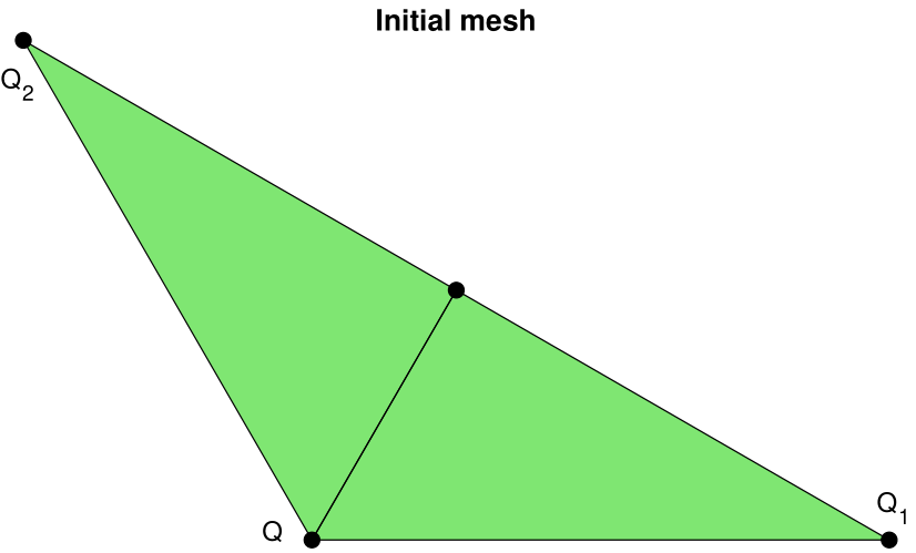
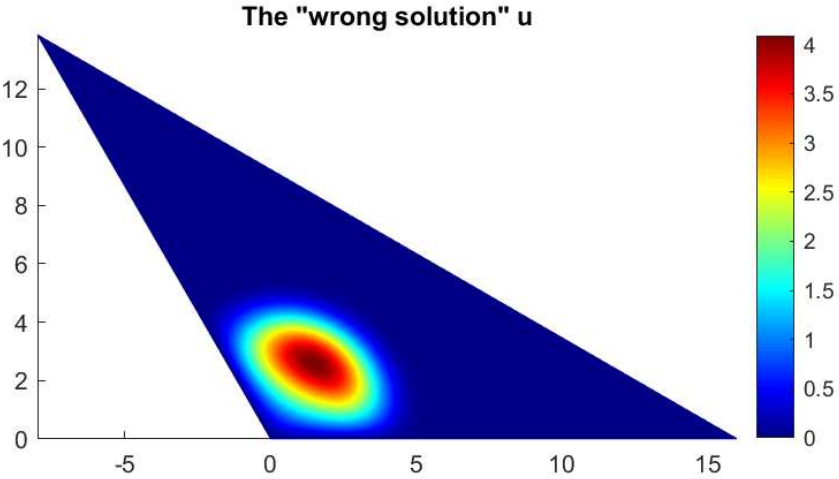
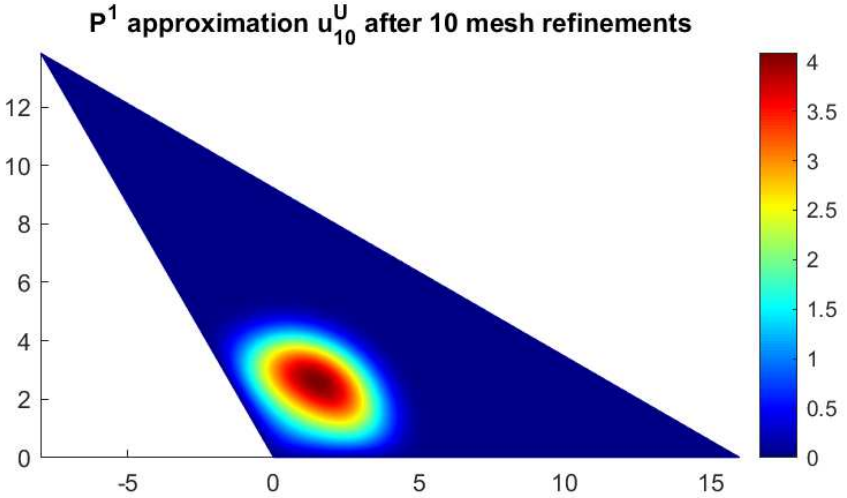
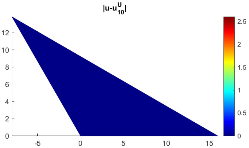
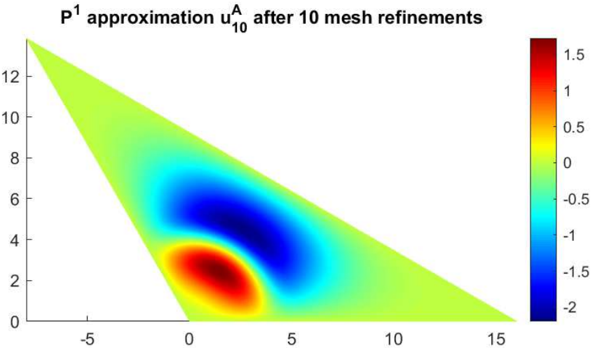
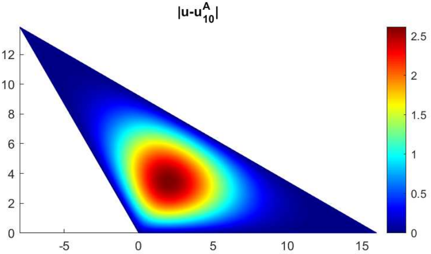
Figure 2. Example 4.1 Test case 1: (a) the domain and the initial mesh; (b) the “wrong solution” $u$; (c) the direct mixed finite element solution $u^{U}_{10}$; (d) the difference $|u-u^{U}_{10}|$; (e) the solution $u^{A}_{10}$ from Algorithm 3.1; (f) the difference $|u-u^{A}_{10}|$.

Table 4. The $H^{1}$ error of the numerical solutions on quasi-uniform meshes.

	$j=7$	$j=8$	$j=9$	$j=10$
$\|u-u_{j}^{U}\|_{H^{1}(\Omega)}$	2.74964e-01	1.35594e-01	6.77391e-02	3.38605e-02
$\|u-u_{j}^{A}\|_{H^{1}(\Omega)}$	6.07564	6.02331	6.00958	6.00306

Test case 2. Here, we consider the domain $\Omega$ to be the polygon with vertices $Q(0,0)$, $Q_{1}(\frac{16\sqrt{3}}{3},0)$, $Q_{2}(\frac{16-8\sqrt{2}}{1+\sqrt{3}},\frac{16-8\sqrt{2}}{1+\sqrt{3}}+8\sqrt{2})$, $Q_{3}(-8\frac{\sqrt{2}+\frac{2\sqrt{3}}{2}}{1+\frac{1}{\sqrt{3}}},8\sqrt{2}-8\frac{\sqrt{2}+\frac{2\sqrt{3}}{2}}{1+\frac{1}{\sqrt{3}}})$ and $Q_{4}(-\frac{8}{3},-4\sqrt{3})$. Then we have $\omega=\angle Q_{1}QQ_{4}\approx 1.383\pi\in(\pi,\frac{3\pi}{2})$. The domain $\Omega$ with the initial mesh is shown in Figure 3(a), and the “wrong solution” $u$ is shown in Figure 3(b).

The direct mixed finite element solution $u_{10}^{U}$ and the difference $|u-u_{10}^{U}|$ are shown in Figure 3(c) and Figure 3(d), respectively. The error $\|u-u_{j}^{U}\|_{H^{1}(\Omega)}$ is shown in Table 5. These results imply that the direct mixed finite element solution converges to the “wrong solution” $u\not\in H^{3}(\Omega)$. On the other hand, since $\omega\in(\pi,\frac{3\pi}{2})$, we have $N=2$ in Algorithm 3.1. The solution $u_{10}^{A}$ of Algorithm 3.1 and the difference $|u-u_{10}^{A}|$ are shown in Figure 3(e) and Figure 3(f), respectively. The error $\|u-u_{j}^{A}\|_{H^{1}(\Omega)}$ is shown in Table 5. These results imply that the solution of Algorithm 3.1 does not converge to the “wrong solution”.

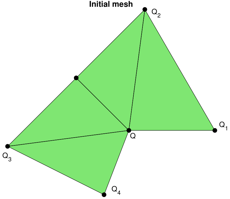
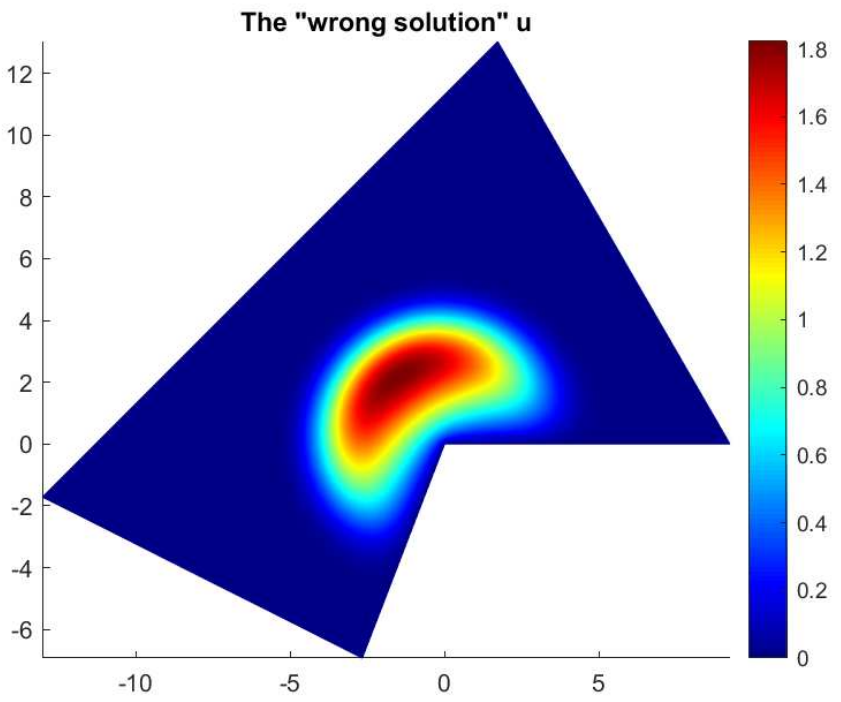
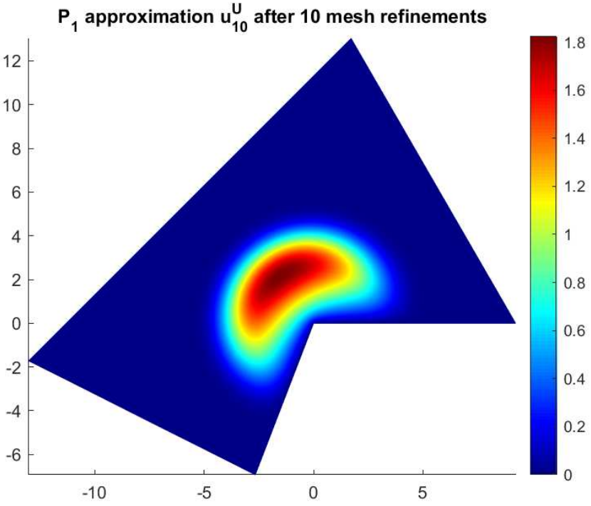
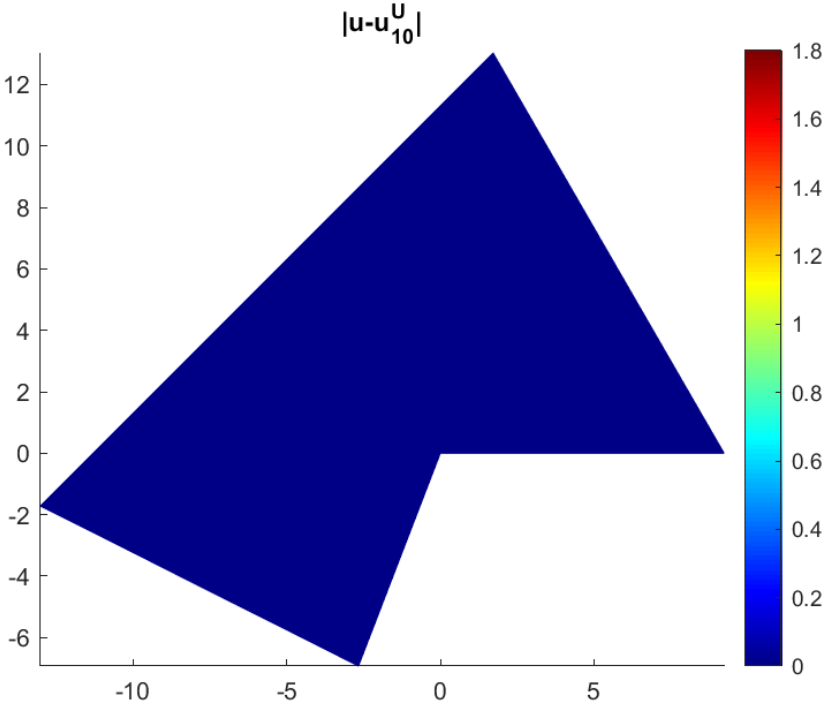
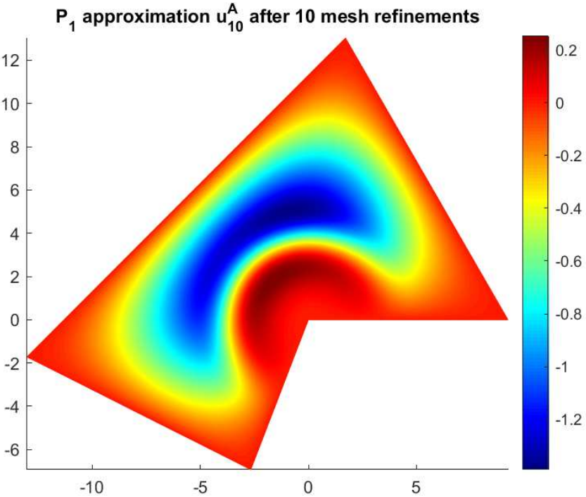
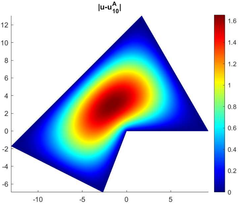
Figure 3. Example 4.1 Test case 2: (a) the domain and the initial mesh; (b) the “wrong solution” $u$; (c) the direct mixed finite element solution $u^{U}_{10}$; (d) the difference $|u-u^{U}_{10}|$; (e) the solution $u^{A}_{10}$ from Algorithm 3.1; (f) the difference $|u-u^{A}_{10}|$.

Table 5. The $H^{1}$ error of the numerical solutions on quasi-uniform meshes.

	$j=7$	$j=8$	$j=9$	$j=10$
$\|u-u_{j}^{U}\|_{H^{1}(\Omega)}$	1.43517e-01	7.44186e-02	3.94988e-02	2.13310e-02
$\|u-u_{j}^{A}\|_{H^{1}(\Omega)}$	4.08611	4.08457	4.08383	4.08329

Test case 3. Consider the polygonal domain $\Omega$ with vertices $Q(0,0)$, $Q_{1}(\frac{16\sqrt{3}}{3},0)$, $Q_{2}(\frac{16-8\sqrt{2}}{1+\sqrt{3}},\frac{16-8\sqrt{2}}{1+\sqrt{3}}+8\sqrt{2})$, $Q_{3}(-8\frac{\sqrt{2}+\frac{2\sqrt{3}}{2}}{1+\frac{1}{\sqrt{3}}},8\sqrt{2}-8\frac{\sqrt{2}+\frac{2\sqrt{3}}{2}}{1+\frac{1}{\sqrt{3}}})$ and $Q_{4}(4,-8\sqrt{3})$. Then we have $\omega=\angle Q_{1}QQ_{4}\approx 1.589\pi\in(\frac{3\pi}{2},2\pi)$. The domain $\Omega$ with the initial mesh is shown in Figure 4(a), and the “wrong solution” $u$ is shown in Figure 4(b).

The direct mixed finite element solution $u_{10}^{U}$ and the difference $|u-u_{10}^{U}|$ are shown in Figure 4(c) and Figure 4(d), respectively. The error $\|u-u_{j}^{U}\|_{H^{1}(\Omega)}$ is shown in Table 6. These results continue to indicate that the direct mixed finite element solution converges to the “wrong solution” $u\not\in H^{3}(\Omega)$. On the other hand, since $\omega\in(\frac{3\pi}{2},2\pi)$, it follows $N=3$ in Algorithm 3.1. The solution $u_{10}^{A}$ of Algorithm 3.1 and the difference $|u-u_{10}^{A}|$ are shown in Figure 4(e) and Figure 4(f), respectively. The error $\|u-u_{j}^{A}\|_{H^{1}(\Omega)}$ is shown in Table 6. These results confirm that the solution of Algorithm 3.1 does not converge to the “wrong solution”.

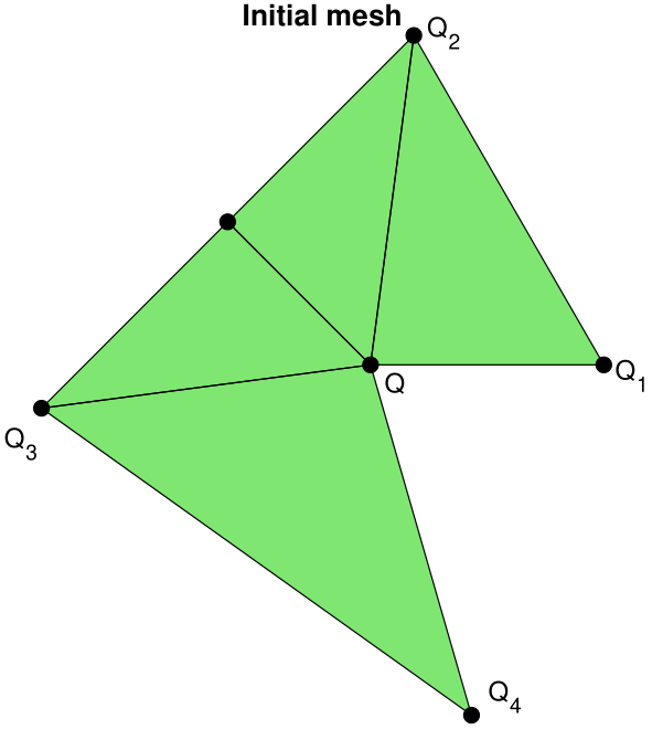
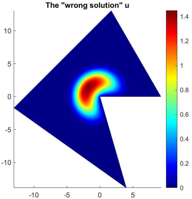
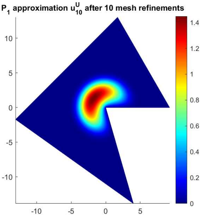
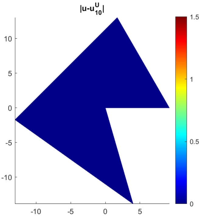
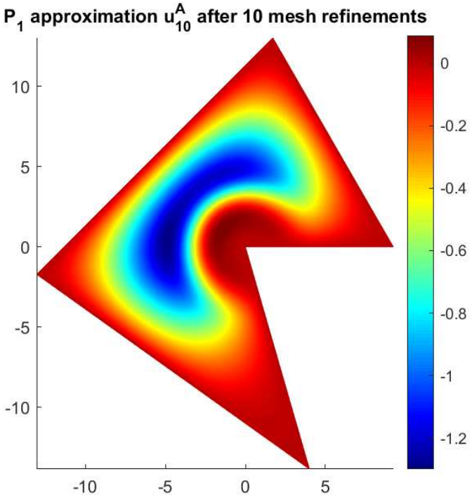
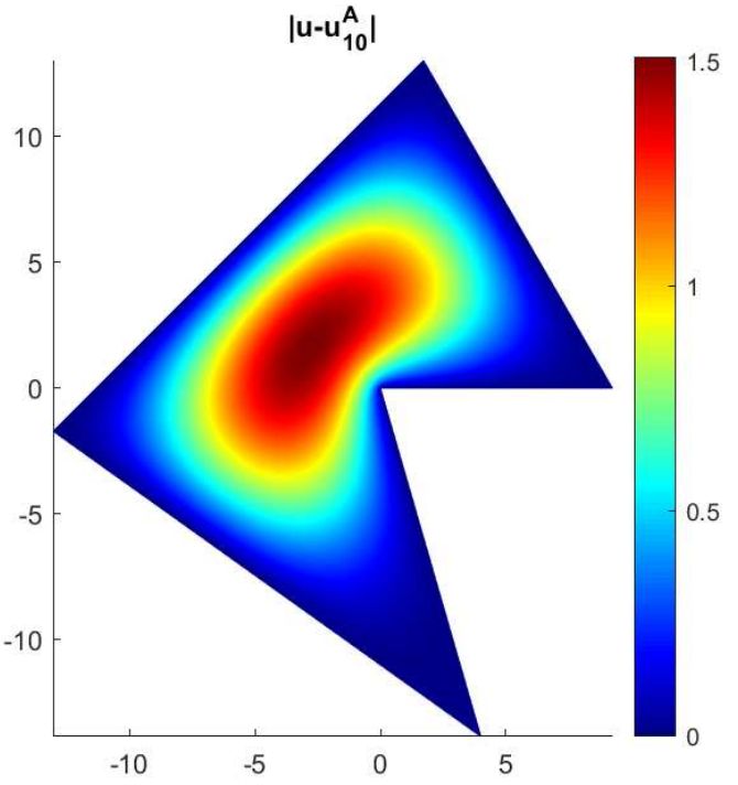
Figure 4. Example 4.1 Test Case 3: (a) the domain and the initial mesh; (b) the “wrong solution” $u$; (c) the direct mixed finite element solution $u^{U}_{10}$; (d) the difference $|u-u^{U}_{10}|$; (e) the solution $u^{A}_{10}$ from Algorithm 3.1; (f) the difference $|u-u^{A}_{10}|$.

Table 6. The $H^{1}$ error of the numerical solutions on quasi-uniform meshes.

	$j=7$	$j=8$	$j=9$	$j=10$
$\|u-u_{j}^{U}\|_{H^{1}(\Omega)}$	1.474223e-01	8.67096e-02	5.25520e-02	3.25455e-02
$\|u-u_{j}^{A}\|_{H^{1}(\Omega)}$	3.863711	3.85981	3.85832	3.85767

Example 4.2.

We solve the triharmonic problem in Example 4.1 again using the direct mixed finite element method and Algorithm 3.1 on quasi-uniform meshes. Here, we take the solution $u_{ex}$ of the following Poisson problem as the exact solution,

$$-\Delta u_{ex}=f_{0}-\sum_{i=1}^{N}c_{i}\sigma_{i}\text{ in }\Omega,\qquad u_{ex}=0\text{ on }\partial\Omega,$$ (4.9)

where

$$f_{0}=-\Delta\left(\tilde{\eta}(r;\tau,R)r^{\frac{N\pi}{\omega}}\sin\left(\frac{N\pi}{\omega}\theta\right)\right)\in H_{0}^{1}(\Omega),$$

with $\tilde{\eta}(r;\tau,R)$ given in (4.8), $\sigma_{i}$ given in (2.15), and $c_{i}$ is the solution of the linear system (2.23). Note that the function $f_{0}=-\Delta u$ for $u$ in (4.4). By Lemma 2.15, we have $u_{ex}\in H^{3}(\Omega)$ and it satisfies

$$-\Delta^{3}u_{ex}=-\Delta^{2}(\Delta u_{ex})=\Delta^{2}f_{0}-\sum_{i=1}^{N}c_{i}\Delta^{2}\sigma_{i}=\Delta^{2}f_{0}=-\Delta^{2}(\Delta u)=-\Delta(\Delta(\Delta u))=f,$$

where we have used the result in Lemma 2.6. Here, the source term $f$ is the same as that in Example 4.1. The purpose of this example is to test the convergence of the direct mixed finite element method and Algorithm 3.1 to the exact solution $u_{ex}$ in (4.9). From Test case 2 to Test case 4, we will use the finite element method solution $u_{exn}$ (instead of using the complicated notation $u_{ex,n+1}$) of (4.9) on mesh $\mathcal{T}_{n+1}$ as an approximation of $u_{ex}$.

Test case 1. Take $\Omega$ as the triangle $\vartriangle QQ_{1}Q_{2}$ with $Q(0,0)$, $Q_{1}(8,0)$ and $Q_{2}(4,4\sqrt{3})$. In this case, the exact solution $u_{ex}=u$ for a given $u$ in (4.4), and its contour is given in Figure 5(a). Here, $\omega=\angle Q_{1}QQ_{2}=\frac{\pi}{3}\in(0,\frac{\pi}{2})$. Thus Algorithm 3.1 coincides with the direct mixed finite element method. The solution $u_{10}^{A}(=u_{10}^{U})$ from Algorithm 3.1 and the difference $|u-u_{10}^{A}|$ are shown in Figure 5(b) and Figure 5(c), respectively. The error $\|u-u_{j}^{A}\|_{H^{1}(\Omega)}$ and convergence rate $\mathcal{R}$ are shown in Table 7. These results show that the solution of Algorithm 3.1 converges to the exact solution in the optimal convergence rate $\mathcal{R}=1$, which coincides with the result in Theorem 3.10 or Table 3.

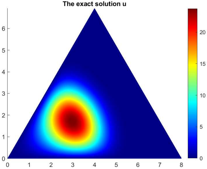
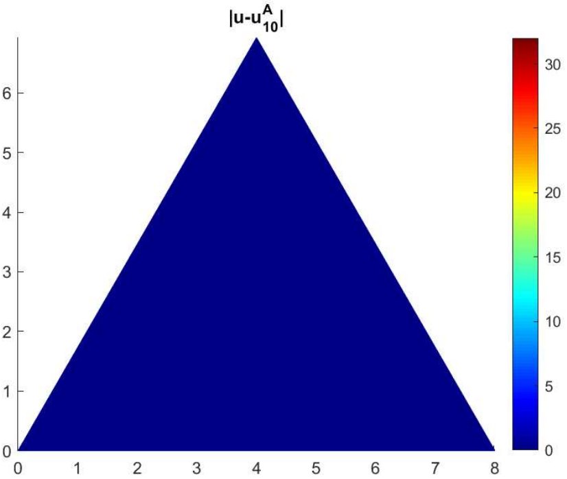
Figure 5. Example 4.2 Test case 1: (a) the exact solution $u$; (b) the solution $u^{A}_{10}$ from Algorithm 3.1; (c) the difference $|u-u^{A}_{10}|$.

Table 7. The $H^{1}$ error and convergence rate $\mathcal{R}$ for Example 4.2 Test case 1.

	$j=5$	$j=6$	$j=7$	$j=8$
$\|u-u_{j}^{A}\|_{H^{1}(\Omega)}$	1.09202	5.45465e-01	2.72663e-01	1.36323e-01
$\mathcal{R}$	$--$	1.00	1.00	1.00

Test case 2. We consider the same domain and initial mesh (see Figure 2(a)) as Test case 1 in Example 4.1. Note that $\omega=\angle Q_{1}QQ_{2}=\frac{2\pi}{3}\in(\frac{\pi}{2},\pi)$. The finite element solution $u_{exn}$ of the exact solution $u_{ex}$ is shown in Figure 6(a). The direct mixed finite element solution $u_{10}^{U}$ and the difference $|u_{exn}-u_{10}^{U}|$ are shown in Figure 2(c) and Figure 6(b), respectively. The error $\|u_{exn}-u_{j}^{U}\|_{H^{1}(\Omega)}$ is shown in Table 8. These results indicate that the direct mixed finite element solution does not converge to the exact solution. Note that $N=1$ in Algorithm 3.1, the solution $u_{10}^{A}$ from Algorithm 3.1 and the difference $|u_{exn}-u_{10}^{A}|$ are shown in Figure 2(e) and Figure 6(c), respectively. The error $\|u_{exn}-u_{j}^{A}\|_{H^{1}(\Omega)}$ is shown in Table 8. These results imply that the solution of Algorithm 3.1 converges to the exact solution.

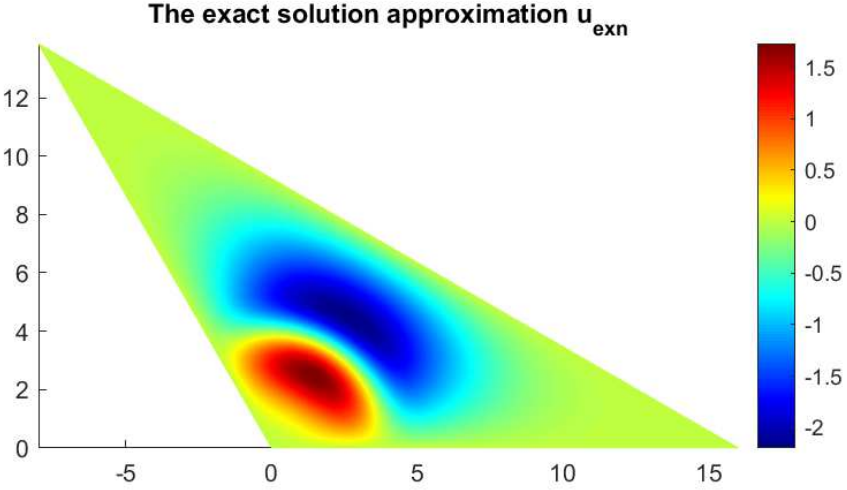
Figure 6. Example 4.2 Test case 2: (a) the exact solution approximation $u$; (b) the difference $|u_{exn}-u^{U}_{10}|$; (c) the difference $|u_{exn}-u^{A}_{10}|$.

Table 8. The $H^{1}$ error of the numerical solutions on quasi-uniform meshes.

	$j=6$	$j=7$	$j=8$	$j=9$
$\|u_{exn}-u_{j}^{U}\|_{H^{1}(\Omega)}$	5.98206	6.01120	6.00363	5.99948
$\|u_{exn}-u_{j}^{A}\|_{H^{1}(\Omega)}$	5.67208e-02	1.47272e-02	6.62074e-03	3.43917e-03

Test case 3. We consider the same domain and initial mesh (see Figure 3(a)) as Test case 2 in Example 4.1. Recall that $\omega=\angle Q_{1}QQ_{4}\approx 1.383\pi\in(\pi,\frac{3\pi}{2})$. The exact solution $u_{exn}$ is shown in Figure 7(a). The direct mixed finite element solution $u_{10}^{U}$ and the difference $|u_{exn}-u_{10}^{U}|$ are shown in Figure 3(c) and Figure 7(b), respectively. The error $\|u_{exn}-u_{j}^{U}\|_{H^{1}(\Omega)}$ is shown in Table 9. These results indicate that the direct mixed finite element solution does not converge to the exact solution. Note that $N=2$ in Algorithm 3.1 in this case. The solution $u_{10}^{A}$ of Algorithm 3.1 and the difference $|u_{exn}-u_{10}^{A}|$ are shown in Figure 3(e) and Figure 7(c), respectively. The error $\|u_{exn}-u_{j}^{A}\|_{H^{1}(\Omega)}$ is shown in Table 9. These results also imply that the solution of Algorithm 3.1 converges to the exact solution.

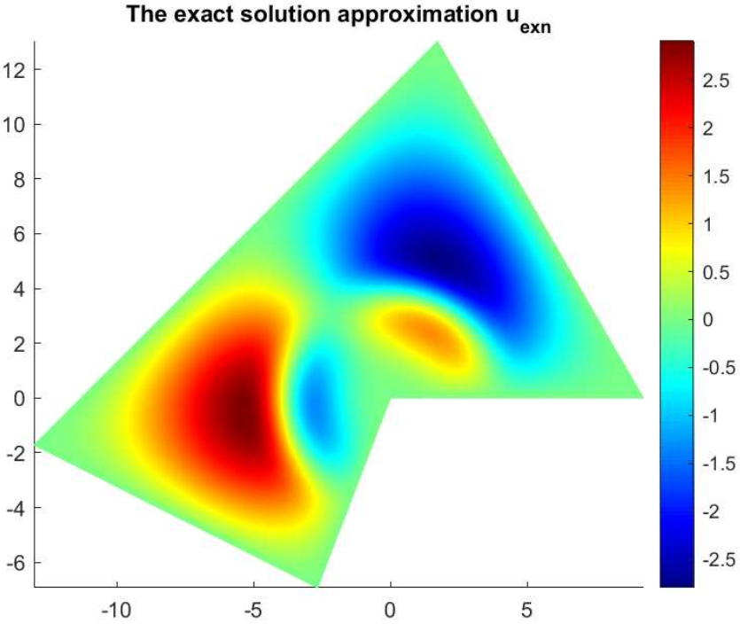
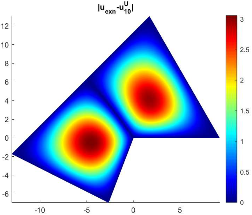
Figure 7. Example 4.2 Test case 3: (a) the exact solution u; (b) the difference $|u_{exn}-u^{U}_{10}|$; (c) the difference $|u_{exn}-u^{A}_{10}|$.

Table 9. The $H^{1}$ error of the numerical solutions on quasi-uniform meshes.

	$j=6$	$j=7$	$j=8$	$j=9$
$\|u_{exn}-u_{j}^{U}\|_{H^{1}(\Omega)}$	9.67666	9.64665	9.63404	9.63164
$\|u_{exn}-u_{j}^{A}\|_{H^{1}(\Omega)}$	5.27303e-02	2.09405e-02	1.01081e-02	4.20655e-03

Test case 4. We consider the same domain and initial mesh (see Figure 4(a)) as Test case 3 in Example 4.1. Recall that $\omega=\angle Q_{1}QQ_{4}\approx 1.589\pi\in(\frac{3\pi}{2},2\pi)$. The approximation $u_{exn}$ of the exact solution is shown in Figure 8(a). The direct mixed finite element solution $u_{10}^{U}$ and the difference $|u_{exn}-u_{10}^{U}|$ are shown in Figure 4(c) and Figure 8(b), respectively. The error $\|u_{exn}-u_{j}^{U}\|_{H^{1}(\Omega)}$ is shown in Table 6. These results continue to indicate that the direct mixed finite element solution does not converge to the exact solution. Note that $N=3$ in Algorithm 3.1, the solution $u_{10}^{A}$ of Algorithm 3.1 and the difference $|u_{exn}-u_{10}^{A}|$ are shown in Figure 4(e) and Figure 8(c), respectively. The error $\|u_{exn}-u_{j}^{A}\|_{H^{1}(\Omega)}$ is shown in Table 10. These results confirm that the solution of Algorithm 3.1 converges to the exact solution.

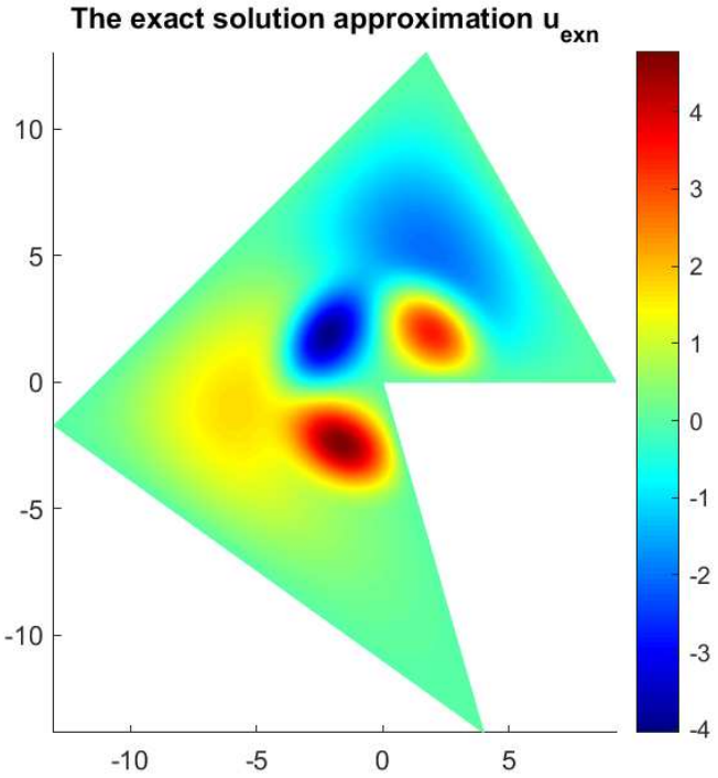
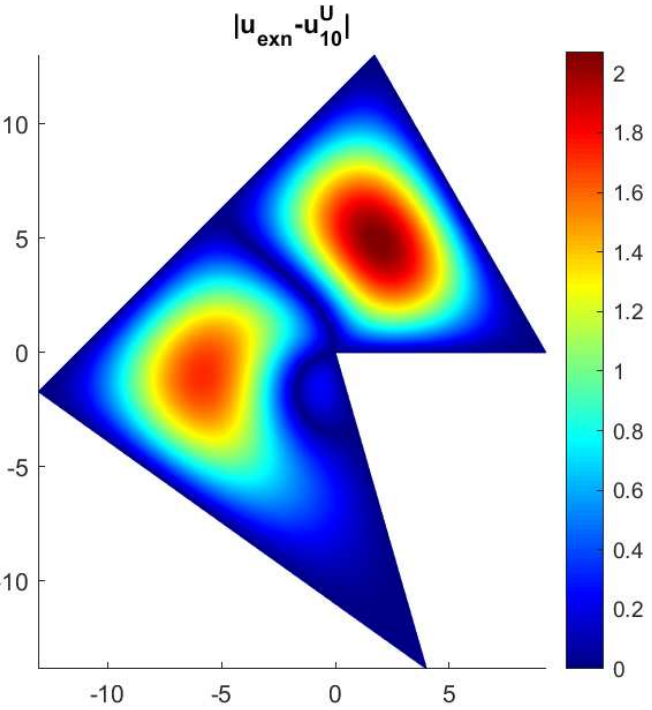
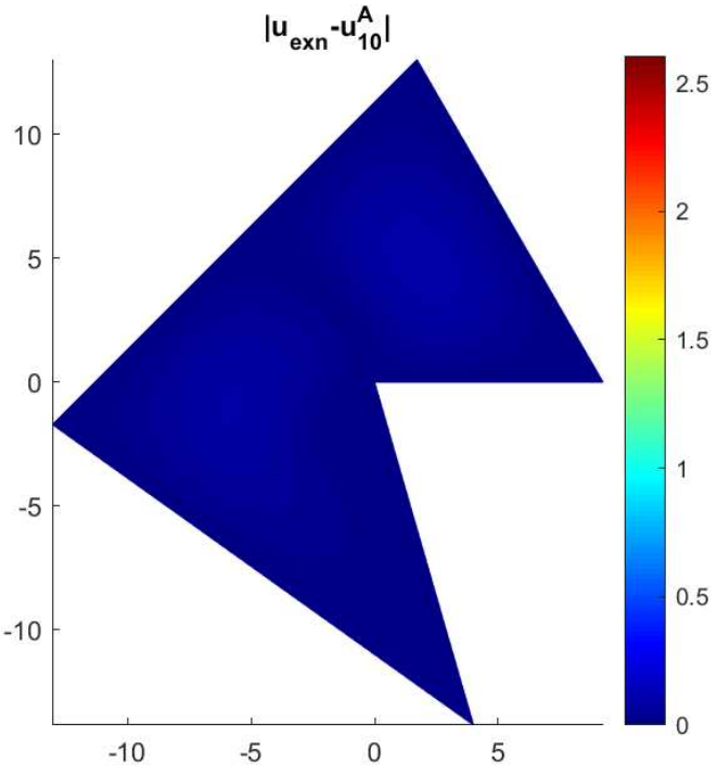
Figure 8. Example 4.2 Test case 4: (a) the exact solution $u$; (b) the difference $|u_{exn}-u^{U}_{10}|$; (c) the difference $|u_{exn}-u^{A}_{10}|$.

Table 10. The $H^{1}$ error of the numerical solutions on quasi-uniform meshes.

	$j=6$	$j=7$	$j=8$	$j=9$
$\|u_{exn}-u_{j}^{U}\|_{H^{1}(\Omega)}$	7.47470	6.98223	6.60342	6.31031
$\|u_{exn}-u_{j}^{A}\|_{H^{1}(\Omega)}$	6.79611e-01	4.98616e-01	3.78626e-01	2.93364e-01

Example 4.3.

In this example, we investigate the convergence of Algorithm 3.1 by considering equation (1.1) with $f=\sin\left(\frac{N\pi}{\omega}\theta\right)$ on different domains with angle $\omega$ categorized in Theorem 3.10 or Table 3, where $N$ is shown in Table 1. For $\omega<\frac{\pi}{2}$, the numerical test on convergence rate can be found in Example 4.2 Test case 1. In the rest of this example, we focus on $\omega>\frac{\pi}{2}$.

Test case 1. Take $\Omega$ as the triangle $\vartriangle QQ_{1}Q_{2}$ with $Q(0,0)$, $Q_{1}(16,0)$ and $Q_{2}(16x_{0},16\sqrt{1-x_{0}^{2}})$ for some $|x_{0}|<1$. The convergence rates for different $\omega=\angle Q_{1}QQ_{2}\in(\frac{\pi}{2},\pi)$ determined by choosing different $x_{0}$ are shown in Table 11. Here, $R=\frac{24}{5}$, $\tau=\frac{1}{8}$ are used when $x_{0}=-0.8$, and default values are used for other cases. The results show that the convergence rate is not optimal when $\omega<\frac{2\pi}{3}$, and it is optimal when $\omega\in[\frac{2\pi}{3},\pi)$. These results are consistent with the expected convergence rate $\mathcal{R}$ in Theorem 3.10 or Table 3 for $\omega\in(\frac{\pi}{2},\pi)$.

Table 11. The $H^{1}$ error for $\omega\in(\frac{\pi}{2},\pi)$ on quasi-uniform meshes.

parameter $x_{0}$	$\omega$	expected rate	$j=7$	$j=8$	$j=9$	$j=10$
$-0.2$	$\approx 0.56409\pi$	$0.46$	0.75	0.67	0.59	0.54
$-0.4$	$\approx 0.63099\pi$	$0.83$	0.96	0.95	0.94	0.93
$-0.5$	$\frac{2\pi}{3}$	$1.00$	1.03	1.01	1.00	1.00
$-0.6$	$\approx 0.70483\pi$	1.00	1.01	1.01	1.01	1.00
$-0.8$	$\approx 0.79517\pi$	1.00	1.02	1.01	1.01	1.00

Test case 2. We consider the polygon $\Omega$ with vertices $Q(0,0)$, $Q_{1}(16,0)$, $Q_{2}(-8,8\sqrt{3})$, and $Q_{3}(-8,-8y_{0}\sqrt{3})$ for some $y_{0}\in(0,1]$, which gives $\omega=\angle Q_{1}QQ_{3}\in(\pi,\frac{4\pi}{3}]$. We then consider the domain $\Omega$ (see Figure 4(a)) presented in Example 4.1 Test case 2, and the corresponding angle $\omega\in(\frac{4\pi}{3},\frac{3\pi}{2})$. The convergence rates for different $\omega\in(\pi,\frac{3\pi}{2})$ are shown in Table 12. The results show that the convergence rate is not optimal when $\omega<\frac{4\pi}{3}$, and it is optimal when $\omega\in[\frac{4\pi}{3},\frac{3\pi}{2})$. These results are consistent with the expected convergence rate in Theorem 3.10 or Table 3 for $\omega\in(\pi,\frac{3\pi}{2})$.

Table 12. The $H^{1}$ error for $\omega\in(\pi,\frac{3\pi}{2})$ on quasi-uniform meshes.

parameter $y_{0}$ or domain	$\omega$	expected rate	$j=6$	$j=7$	$j=8$	$j=9$
$0.2$	$\approx 1.10615\pi$	$0.38$	0.82	0.72	0.62	0.53
$0.6$	$\approx 1.25612\pi$	$0.82$	0.96	0.95	0.94	0.93
$0.8$	$\approx 1.30101\pi$	$0.93$	0.98	0.98	0.98	0.98
$1.0$	$\frac{4\pi}{3}$	1.00	1.00	1.00	1.00	1.00
$\Omega$ in Figure 4(a)	$\approx 1.38305\pi$	1.00	1.02	1.02	1.01	1.01

Test case 3. We consider the polygon $\Omega$ with vertices $Q(0,0)$, $Q_{1}(\frac{16\sqrt{3}}{3},0)$, $Q_{2}(\frac{16-8\sqrt{2}}{1+\sqrt{3}},\frac{16-8\sqrt{2}}{1+\sqrt{3}}+8\sqrt{2})$, $Q_{3}(-8\frac{\sqrt{2}+\frac{2\sqrt{3}}{2}}{1+\frac{1}{\sqrt{3}}},8\sqrt{2}-8\frac{\sqrt{2}+\frac{2\sqrt{3}}{2}}{1+\frac{1}{\sqrt{3}}})$, and $Q_{4}(x_{1},-8\sqrt{3})$ for some $x_{1}\in(0,8\sqrt{3}]$, which generates $\omega=\angle Q_{1}QQ_{4}\in(\frac{3\pi}{2},\frac{7\pi}{4}]$. The convergence rates for different $\omega\in(\frac{3\pi}{2},2\pi)$ are shown in Table 13. These results are consistent with the expected convergence rate in Theorem 3.10 or Table 3 for $\omega\in(\frac{3\pi}{2},2\pi)$.

Table 13. The $H^{1}$ error for $\omega\in(\frac{3\pi}{2},2\pi)$ on quasi-uniform meshes.

$x_{1}$ or domain	$\omega$	expected rate	$j=6$	$j=7$	$j=8$	$j=9$
$x_{1}=4$	$\approx 1.58946\pi$	$0.23$	0.87	0.76	0.63	0.50
$x_{1}=8$	$\frac{5\pi}{3}$	$0.40$	0.83	0.75	0.65	0.60
$x_{1}=8\sqrt{3}$	$\frac{7\pi}{4}$	$0.57$	0.87	0.82	0.77	0.71

References

- [1] R. Backofen, A. Rätz, and A. Voigt. Nucleation and growth by a phase field crystal (PFC) model. Philosophical Magazine Letters, 87(11):813–820, 2007.
- [2] J. W. Barrett, S. Langdon, and R. Nürnberg. Finite element approximation of a sixth order nonlinear degenerate parabolic equation. Numerische Mathematik, 96(3):401–434, 2004.
- [3] J. H. Bramble and M. Zlámal. Triangular elements in the finite element method. Mathematics of Computation, 24(112):809–820, 1970.
- [4] S. C. Brenner and L. R. Scott. The Mathematical Theory of Finite Element Methods, volume 15 of Texts in Applied Mathematics. Springer-Verlag, New York, second edition, 2002.
- [5] M. Cheng and J. A. Warren. An efficient algorithm for solving the phase field crystal model. Journal of Computational Physics, 227(12):6241–6248, 2008.
- [6] P. Ciarlet. The Finite Element Method for Elliptic Problems, volume 4 of Studies in Mathematics and Its Applications. North-Holland, Amsterdam, 1978.
- [7] J. Droniou, M. Ilyas, B. P. Lamichhane, and G. E. Wheeler. A mixed finite element method for a sixth-order elliptic problem. IMA Journal of Numerical Analysis, 39(1):374–397, 2019.
- [8] L. Evans. Partial Differential Equations, volume 19 of Graduate Studies in Mathematics. AMS, Rhode Island, 1998.
- [9] P. Grisvard. Elliptic Problems in Nonsmooth Domains. Pitman, Boston, 1985.
- [10] P. Grisvard. Singularities in Boundary Value Problems, volume 22 of Research Notes in Applied Mathematics. Springer-Verlag, New York, 1992.
- [11] T. Gudi and M. Neilan. An interior penalty method for a sixth-order elliptic equation. IMA journal of numerical analysis, 31(4):1734–1753, 2011.
- [12] Z. Hu, S. M. Wise, C. Wang, and J. S. Lowengrub. Stable and efficient finite-difference nonlinear-multigrid schemes for the phase field crystal equation. Journal of Computational Physics, 228(15):5323–5339, 2009.
- [13] V.A. Kondrat′ev. Boundary value problems for elliptic equations in domains with conical or angular points. Trudy Moskov. Mat. Obšč., 16:209–292, 1967.
- [14] V. Kozlov, V. Maz′ya, and J. Rossmann. Elliptic boundary value problems in domains with point singularities, volume 52 of Mathematical Surveys and Monographs. American Mathematical Society, Providence, RI, 1997.
- [15] V. Kozlov, V. Maz′ya, and J. Rossmann. Spectral problems associated with corner singularities of solutions to elliptic equations, volume 85 of Mathematical Surveys and Monographs. American Mathematical Society, Providence, RI, 2001.
- [16] H. Li. Graded Finite Element Methods for Elliptic Problems in Nonsmooth Domains. Surveys and Tutorials in the Applied Mathematical Sciences (STAMS, volume 10). Springer, 2022.
- [17] H. Li and S. Nicaise. Regularity and a priori error analysis on anisotropic meshes of a Dirichlet problem in polyhedral domains. Numer. Math., 139(1):47–92, 2018.
- [18] H. Li, P. Yin, and Z. Zhang. A finite element method for the biharmonic problem with Navier boundary conditions in a polygonal domain. IMA Journal of Numerical Analysis, pages 1–23, 2022. https://doi.org/10.1093/imanum/drac026.
- [19] S. Nazarov and B. A. Plamenevsky. Elliptic Problems in Domains with Piecewise Smooth Boundaries, volume 13. Walter de Gruyter, 1994.
- [20] S.A. Nazarov and G. Kh. Svirs. Boundary value problems for the biharmonic equation and the iterated Laplacian in a three-dimensional domain with an edge. Zap. Nauchn. Sem. S.-Peterburg. Otdel. Mat. Inst. Steklov. (POMI), 336(Kraev. Zadachi Mat. Fiz. i Smezh. Vopr. Teor. Funkts. 37):153–198, 276–277, 2006.
- [21] H. Ugail. Partial Differential Equations for Geometric Design. Springer Science & Business Media, 2011.
- [22] A. Ženíšek. Interpolation polynomials on the triangle. Numerische Mathematik, 15:283–296, 1970.
- [23] S. M. Wise, C. Wang, and J. S. Lowengrub. An energy-stable and convergent finite-difference scheme for the phase field crystal equation. SIAM Journal on Numerical Analysis, 47(3):2269–2288, 2009.
- [24] S. Wu and J. Xu. interior penalty nonconforming finite element methods for -th order pdes in . arXiv preprint arXiv:1710.07678, 2017.
- [25] S. Wu and J. Xu. Nonconforming finite element spaces for th order partial differential equations on simplicial grids when . Mathematics of Computation, 88(316):531–551, 2019.
- [26] S. Zhang and Z. Zhang. Invalidity of decoupling a biharmonic equation to two Poisson equations on non-convex polygons. Int. J. Numer. Anal. Model., 5(1):73–76, 2008.