Spectral Subspaces of Sturm-Liouville Operators and Variable Bandwidth

Abstract.

We study spectral subspaces of the Sturm-Liouville operator $f\mapsto-(pf^{\prime})^{\prime}$ on $\mathbb{R}$, where $p$ is a positive, piecewise constant function. Functions in these subspaces can be thought of as having a local bandwidth determined by $1/\sqrt{p}$. Using the spectral theory of Sturm-Liouville operators, we make the reproducing kernel of these spectral subspaces more explicit and compute it completely in certain cases. As a contribution to sampling theory, we then prove necessary density conditions for sampling and interpolation in these subspaces and determine the critical density that separates sets of stable sampling from sets of interpolation.

1. Introduction

In [9] we proposed a new notion of variable bandwidth that connects the theory of Sturm-Liouville operators on $\mathbb{R}$ with notions from signal processing. Roughly speaking, bandwidth is the largest frequency $\Omega$ in a signal (or function) $f$ on the real line, so that $f$ can be represented as $f(x)=\int_{-\Omega}^{\Omega}\hat{f}(\lambda)e^{i\lambda x}\,d\lambda$ via the inverse Fourier transform. Intuitively it makes sense to speak of a maximum frequency near a time $x$ or, in other words, of variable bandwidth. However, a precise mathematical formulation of variable bandwidth seems difficult. The engineering literature offers several informal definitions [3, 5, 11, 19], but so far none of them has become accepted. The mathematical approach in  [1, 2] only yields a class of new norms on Sobolev spaces and lacks the fundamental features of bandwidth. The attempt of Kempf and Martin [14] uses self-adjoint extensions of a differential operator for an algorithmic approach to variable bandwidth.

Our idea in [9] was to define variable bandwidth by means of the spectral subspaces of a Sturm-Liouville operator on $\mathbb{R}$ which is closely related to the work of Pesenson and Zayed on abstract Paley-Wiener spaces ([12, 15], see also [18]). Precisely, let $p>0$ be a strictly positive, sufficiently smooth function on $\mathbb{R}$ and consider the Sturm-Liouville operator $A_{p}f=-(pf^{\prime})^{\prime}$ on a suitable domain in $L^{2}(\mathbb{R})$ so that $A_{p}$ is a positive self-adjoint operator. The spectral theorem asserts the existence of a projection-valued measure $\Lambda\mapsto\chi_{\Lambda}(A_{p})$. In  [9] we argued that the range of such an orthogonal projection is a good model for variable bandwidth and defined the Paley-Wiener space (in engineering language this is a space of bandlimited functions) as

$$PW_{[0,\Omega]}\left(A_{p}\right)=\chi_{[0,\Omega]}\left(A_{p}\right)L^{2}\left(\mathbb{R}\right)\,.$$

For a general Borel set $\Lambda\subset[0,\infty)$ of finite measure, we write $PW_{\Lambda}(A_{p})=\chi_{\Lambda}(A_{p})L^{2}(\mathbb{R})$ for the corresponding spectral subspace.

Taking $p\equiv 1$ and $A_{p}=-\frac{d^{2}}{dx^{2}}$, we see that the Fourier transform of $A_{p}f$ is $\widehat{A_{p}f}(\xi)=\xi^{2}\hat{f}(\xi)$. Thus spectral values $\xi^{2}\in[0,\Omega]$ correspond to frequencies $\xi\in[-\sqrt{\Omega},\sqrt{\Omega}]$. Consequently, $PW_{[0,\Omega]}(-\frac{d^{2}}{dx^{2}})=\{f\in L^{2}(\mathbb{R}):\operatorname*{supp}\hat{f}\subseteq[-\sqrt{\Omega},\sqrt{\Omega}]\}$ and coincides with the classical space of bandlimited functions with maximum frequency $\sqrt{\Omega}$.

In [9] we proved several general theorems about the general Paley-Wiener spaces $PW_{[0,\Omega]}\left(A_{p}\right)$ to support the interpretation of variable bandwidth. Among these were a general, almost optimal sampling theorem for the reconstruction of a function in $PW_{[0,\Omega]}\left(A_{p}\right)$ from its samples $\{f(x):x\in X\}$ on a discrete set $X\subseteq\mathbb{R}$ and a necessary density condition for sampling. These results indicate that a function in $PW_{[0,\Omega]}\left(A_{p}\right)$ behaves like a function with maximum frequency $(\Omega/p(x))^{1/2}$ near $x$. Thus the function $p$ defining the Sturm-Liouville operator parametrizes the local bandwidth.

Despite the success of the theory and an explicit iterative reconstruction algorithm, an intended numerical implementation faces some immediate and serious difficulties. Even the most naive numerical treatment requires some knowledge of the reproducing kernel, that is, of those functions in $PW_{[0,\Omega]}\left(A_{p}\right)$ that determine the point evaluations $f(x)=\int_{\mathbb{R}}f(y)\overline{k_{x}(y)}\,dy=\langle f,k_{x}\rangle$. Since $PW_{[0,\Omega]}\left(A_{p}\right)$ is a reproducing kernel Hilbert space [9, Prop. 3.3] these functions do exist. But what exactly is this reproducing kernel?

Any deeper investigation of the Paley-Wiener spaces and any attempt of a numerical implementation of a sampling reconstruction must use some knowledge about the reproducing kernel. In a sense the situation is similar to the theory of spaces of analytic functions (Bergman spaces), where some of the deepest results hinge on delicate properties of the reproducing kernel (see [7] for a celebrated example).

Although the spectral projections are natural objects associated to a Sturm-Liouville operator, surprisingly little explicit knowledge seems to be available. A general formula can be derived from spectral theory as follows. Let $\Phi(\lambda,\cdot)=(\Phi^{+}(\lambda,\cdot),\Phi^{-}(\lambda,\cdot))$ be a suitable fundamental system of solutions of $A_{p}f=-(pf^{\prime})^{\prime}=\lambda f$ on $\mathbb{R}$ that depends continuously on $\lambda\in\mathbb{R}$. If $\Lambda\subseteq[0,\infty)$ has finite Lebesgue measure, then there exists a $2\times 2$ positive matrix-valued Borel measure $\mu$ constructed from $\Phi(\lambda,\cdot)$ (see, e.g., [21, Sec. 14] for details), such that the reproducing kernel of $PW_{\Lambda}(A_{p})$ is given by

(1.1) $$k_{\Lambda}(x,y)=k_{x}(y)=\int_{\Lambda}\overline{\Phi(\lambda,x)}\cdot\Phi(\lambda,y)\,d\mu(\lambda)=\langle\Phi(\cdot,y),\Phi(\cdot,x)\rangle_{L^{2}(\Lambda,\mu)}\,.$$

The inner product in $L^{2}([0,\Omega],\mu)$ is

$$\langle F,G\rangle_{L^{2}(\mathbb{R},\mu)}=\int_{\Lambda}F(\lambda)\cdot\overline{G(\lambda)}\,d\mu(x)=\sum_{j,k=1}^{2}\int_{\Lambda}F_{j}(\lambda)\overline{G_{k}(\lambda)}\,d\mu_{jk}(\lambda)$$

where the $\mu_{jk}$’s are the component measures of $\mu$. See [6, Sec. XIII.5] for more details on matrix measures.

In this classical formula the kernel still depends on the knowledge of a fundamental solution and is far from explicit.

In this paper we study the Sturm-Liouville operator $A_{p}f=-(pf^{\prime})^{\prime}$ for a piecewise constant, positive function $p$ and make the reproducing kernel $k$ as explicit as possible. Let $t_{1}<t_{2}<\dots<t_{n}$ be the position of the jumps of $p$ and set $t_{0}=-\infty$ and $t_{n+1}=+\infty$. Then the step function

(1.2) $$p(x)=\sum_{j=0}^{n}p_{j}\chi_{(t_{j},t_{j+1}]}(x)$$

is our model to parametrize variable bandwidth. Indeed, this is the most natural assumption, since it can be shown that for such a parametrizing function the restriction of $f\in PW_{[0,\Omega]}\left(A_{p}\right)$ to an interval $I_{j}=[t_{j},t_{j+1})$ is equal to the restriction of a classical bandlimited function with bandwidth $(\Omega/p_{j})^{1/2}$. This is plausible because the operator $A_{p}$ restricted to $L^{2}(I_{j})$ is just $-p_{j}\frac{d^{2}}{dx^{2}}$ with eigenfunctions $e^{\pm i\lambda x}$ corresponding to the eigenvalues $p_{j}\lambda^{2}$. Consequently a spectral value $p_{j}\lambda^{2}\leq\Omega$ corresponds to a frequency $|\lambda|\leq(\Omega/p_{j})^{1/2}$, cf. [9, Prop. 3.5].

For this natural class of parametrizing functions we can describe the reproducing kernel in a more explicit fashion than in (1.1). Let $\Phi(\lambda,\cdot)=(\Phi^{+}(\lambda,\cdot),\Phi^{-}(\lambda,\cdot))$ be a fundamental system of solutions of $A_{p}f=-(pf^{\prime})^{\prime}=\lambda f$ that depends analytically on $\lambda\in\mathbb{C}\setminus(-\infty,0]$. Then the reproducing kernel of $PW_{\Lambda}(A_{p})$ is as follows.

Theorem 1.1.

Let $\Lambda\subset\mathbb{R}_{0}^{+}$ and $p$ be a piecewise constant, positive function as in (1.2). Then $PW_{\Lambda}(A_{p})$ is a reproducing kernel Hilbert space with a kernel of the form

$$k_{\Lambda}(x,y)=\dfrac{1}{2\pi}\sum_{j,k=1}^{n}\chi_{(t_{j},t_{j+1}]}(x)\chi_{(t_{k},t_{k+1}]}(y)\int_{\Lambda^{1/2}}\dfrac{\vartheta_{jk}(u)}{\kappa(u)}\,du,\quad x,y\in\mathbb{R}.$$

All functions $\vartheta_{jk}$ and $\kappa$ depend only on the parameters $\{p_{j}:j=1,\dots,n\}$ and the jumps $\{t_{j}\}$ of $p$. Furthermore, each function $\vartheta_{jk}$ and $\kappa$ are almost periodic polynomials with real coefficients.

For the spectrum $\Lambda=[0,\Omega]$ and $n=2$, i.e., $p$ has two jumps and partitions $\mathbb{R}$ into three intervals of constant local bandwidth, $\kappa$ can be explicitly computed to be (set $q_{k}=p_{k}^{-1/2}$, $k=0,1$)

(1.3) $$\kappa(u)=\tfrac{1}{16q_{0}^{2}}\left[\left(1+\tfrac{q_{0}}{q_{1}}\right)^{2}\left(1+\tfrac{q_{1}}{q_{2}}\right)^{2}+\left(1-\tfrac{q_{0}}{q_{1}}\right)^{2}\left(1-\tfrac{q_{1}}{q_{2}}\right)^{2}\right]+\tfrac{1}{8q_{0}^{2}}\left(1-\tfrac{q_{0}^{2}}{q_{1}^{2}}\right)\left(1-\tfrac{q_{1}^{2}}{q_{2}^{2}}\right)\,\cos 2q_{1}Tu\,.$$

The kernel $k$ is then obtained by evaluating parameter integrals of the form

$$J(s)=\int_{\Lambda^{1/2}}\frac{e^{isu}}{C+K\cos\zeta u}\,du,\quad s\in\mathbb{R}.$$

This integral seems to be a new type of special function. The kernel can then be written explicitly by means of this function $J$. This will be done in Theorem 4.4.

In the second part of the paper we derive necessary density conditions for sampling and interpolation in $PW_{\Lambda}(A_{p})$ in the style of Landau [13] for the case of a piecewise constant parametrizing function $p$. As in [9, Sec. 6], we consider the positive measure

(1.4) $$\mu_{p}([a,b])=\int_{a}^{b}\dfrac{dx}{\sqrt{p(x)}}\,,$$

which is determined by the parametrizing function $p$. We also recall the following notions. We say $X$ is a set of stable sampling for $PW_{\Lambda}(A_{p})$ if there exist $C_{1},C_{2}>0$ such that

$$C_{1}\left\|f\right\|_{2}^{2}\leq\sum_{x\in X}|f(x)|^{2}\leq C_{2}\left\|f\right\|_{2}^{2}\quad\text{ for all }f\in PW_{\Lambda}(A_{p})\,.$$

Furthermore, $X$ is a set of interpolation for $PW_{\Lambda}(A_{p})$ if for every $c\in\ell^{2}(X)$ there exists $f\in PW_{\Lambda}(A_{p})$ such that $f(x)=c_{x}$ for all $x\in X$. Using a modified form of the upper and lower Beurling densities via $\mu_{p}$, we derive the following version of the density theorem.

Theorem 1.2 (Density theorem in $PW_{\Lambda}(A_{p})$).

Let $p$ be a piecewise constant function and $\Omega>0$.

1. If $X$ is a set of stable sampling for $PW_{[0,\Omega]}(A_{p})$, then

   $$D_{p}^{-}(X)=\liminf_{r\to\infty}\inf_{x\in\mathbb{R}}\dfrac{\#(X\cap B_{r}(x))}{\mu_{p}(B_{r}(x))}\geq\frac{\Omega^{1/2}}{\pi}.$$

2. If $X$ is a set of interpolation for $PW_{[0,\Omega]}(A_{p})$, then

   $$D_{p}^{+}(X)=\limsup_{r\to\infty}\sup_{x\in\mathbb{R}}\dfrac{\#(X\cap B_{r}(x))}{\mu_{p}(B_{r}(x))}\leq\frac{\Omega^{1/2}}{\pi}.$$

Although the density theorem does not make any reference to the reproducing kernel, Theorem 1.1 is substantial for its proof. In the proof of Theorem 1.2 we will apply a general density theorem for sampling and interpolation in reproducing kernel Hilbert spaces [8]. This statement identifies an averaged trace of the reproducing kernel as the critical density. Based on the semi-explicit formula of Theorem 1.1 we will show that the averaged trace equals $\sqrt{\Omega}/\pi$ (see Theorem 5.9).

Theorem 1.2 holds for much more general spectra $\Lambda$. In fact, if $\Lambda\subset\mathbb{R}^{+}$ has finite Lebesgue measure, then the necessary condition for sampling is

$$D_{p}^{-}(X)\geq\tfrac{1}{\pi}\big{|}\{x\in\mathbb{R}:x^{2}\in\Lambda\}\big{|}\,,$$

where $|I|$ denotes the Lebesgue measure of a set $I\subseteq\mathbb{R}$.

Finally, the formulation of the necessary densities is identical to the main result in [9, Thm. 6.2, 6.3]. However, the assumptions on the parametrizing function $p$ are radically different. In [9] we assumed $p$ to be smooth, at least $C^{2}$, and then transformed the Sturm-Liouville operator into an equivalent Schrödinger operator and applied scattering theory. In the multivariate version in [10] we even assumed $p\in C^{\infty}$ and used the regularity theory of elliptic partial differential equations to derive information about the reproducing kernel. For the case of a singular function $p$ all these tools fail dramatically; our main tool is the simple form of the operator $A_{p}$ and the ensuing more explicit knowledge about the reproducing kernel.

1.1. Organization

The paper is organized as follows: in Section 2 we recall a few concepts and results from Sturm-Liouville theory. In Section 3 we introduce rigorously the Paley-Wiener space $PW_{\Lambda}(A_{p})$. We will determine a suitable fundamental system of solutions and the spectral measure $\mu$ for $A_{p}$. In Section 4 we compute the reproducing kernel of $PW_{[0,\Omega]}\left(A_{p}\right)$ for a piecewise constant parametrizing function $p$. In Section 5, we derive necessary density conditions for sampling and interpolation in $PW_{\Lambda}(A_{p})$ with piecewise constant $p$.

Acknowledgment: We would like to thank our colleagues Gerald Teschl and Jussi Behrndt for discussion and advice about the spectral theory of Sturm-Liouville operators.

2. Spectral Theory of Sturm-Liouville Operators

This section, adapted from [9], is a brief review of the relevant spectral theory of singular Sturm-Liouville differential expressions on $\mathbb{R}$ in divergence form. Given a positive function $p$ on $\mathbb{R}$, we define the differential expression $\tau_{p}$ by $\tau_{p}f=-\left(pf^{\prime}\right)^{\prime}$.

Proposition 2.1.

If $p$ is a piecewise constant function as defined in (1.2), then $\tau_{p}$ with domain

$$\mathcal{D}(A_{p}) =\{f\in L^{2}(\mathbb{R}):f,pf^{\prime}\in AC_{loc}(\mathbb{R})\textrm{ and }\tau_{p}f\in L^{2}(\mathbb{R})\},$$

$$A_{p}f =\tau_{p}f,f\in\mathcal{D}(A_{p})$$

defines the self-adjoint operator $A_{p}$ on $L^{2}\left(\mathbb{R}\right)$. The spectrum of $A_{p}$ is purely absolutely continuous and consists of the positive semiaxis: $\sigma\left(A_{p}\right)=\sigma_{ac}\left(A_{p}\right)=[0,\infty)$.

Proof.

The assertions concerning self-adjointness are standard, see, e.g., [17, 21, 6]. The result on the purely absolutely continuous spectrum can be inferred form [16].  

We also have the following spectral representation of $A_{p}$ (see [9]).

Proposition 2.2.

If $\Phi(\lambda,x)=\big{(}\phi_{1}(\lambda,x),\phi_{2}(\lambda,x)\big{)}$ is a fundamental system of solutions of $(\tau-\lambda)\phi=0$ that depends continuously on $\lambda$, then there exists a $2\times 2$ matrix measure $\rho$, such that the operator

(2.1) $$\mathcal{F}_{A_{p}}:L^{2}(\mathbb{R})\to L^{2}(\mathbb{R},d\rho);\quad\mathcal{F}_{A_{p}}f(\lambda)=\int_{\mathbb{R}}f(x)\,\overline{\Phi(\lambda,x)}dx$$

is unitary and diagonalizes $A$, i.e.,

$$\mathcal{F}_{A_{p}}A\mathcal{F}_{A_{p}}^{-1}G(\lambda)=\lambda G(\lambda)$$

for all $G\in L^{2}(\mathbb{R},d\rho)$. The inverse has the form

$${\mathcal{F}_{A_{p}}^{-1}}G(x)=\int_{\mathbb{R}}G(\lambda)\cdot{\Phi(\lambda,x)}\,d\rho(\lambda)\,.$$

for $G\in L^{2}(\mathbb{R},d\rho)$.

If $g$ is a bounded Borel function on $\mathbb{R}$, then for every $f\in L^{2}(\mathbb{R})$,

(2.2) $$g(A)f(x)=\int_{\mathbb{R}_{0}^{+}}g(\lambda)\mathcal{F}_{A_{p}}f(\lambda)\cdot{\Phi(\lambda,x)}\,d\rho(\lambda)\,.$$

All integrals $\int_{\mathbb{R}}$ have to be understood as $\lim_{\begin{subarray}{c}a\to-\infty\\ b\to\infty\end{subarray}}\int_{a}^{b}$ with convergence in $L^{2}$.

$\mathcal{F}_{A_{p}}$ is called the spectral transform (or also a spectral representation of $A$).

Remark.

It is always possible to choose a fundamental system of solutions $\Phi(\lambda,\cdot)$ that depends continuously (even analytically) on $\lambda$ [21]. The spectral measure can (and will be) then be constructed explicitly from the knowledge of such a set of fundamental solutions $(A-z)\phi=0$, see [6, 17, 20, 21] .

In particular, the spectral projection $\chi_{\Lambda}(A_{p}):L^{2}(\mathbb{R})\to L^{2}(\mathbb{R})$ corresponding to a Borel set $\Lambda\subseteq\mathbb{R}_{0}^{+}$ is given by

(2.3) $$\chi_{\Lambda}(A_{p})f=\int_{\Lambda}\mathcal{F}_{A_{p}}f(\lambda)\cdot\Phi(\lambda,\cdot)\,d\mu(\lambda)=\mathcal{F}_{A_{p}}^{-1}(\chi_{\Lambda}\mathcal{F}_{A_{p}}f)$$

for all $f\in L^{2}(\mathbb{R})$. With this projection operator we define the main object for our approach to variable bandwidth.

Definition 2.3.

Let $A_{p}$ as defined in Proposition 2.1 and $\Lambda\subset\mathbb{R}_{0}^{+}$ be of finite measure. The Paley-Wiener space, denoted $PW_{\Lambda}(A_{p})$, is the range of $\chi_{\Lambda}(A_{p})$, i.e.,

$$PW_{\Lambda}(A_{p})=\chi_{\Lambda}(A_{p})(L^{2}(\mathbb{R})).$$

Equivalently, a function $f\in L^{2}(\mathbb{R})$ belongs to $PW_{\Lambda}(A_{p})$ if $f=\chi_{\Lambda}(A_{p})f$.

Some elementary properties of functions of variable bandwidth can be found in [9, Sec. 3]. As argued in [9], this definition is one possibility to give meaning to the notion of variable bandwidth.

3. Paley Wiener Space with Piecewise Constant Parametrization

We now present the fundamental results on $PW_{\Lambda}(A_{p})$ for $p$ piecewise constant as in (1.2).We will derive a formula for the spectral measure and discuss a strategy how to compute the reproducing kernel.

3.1. Fundamental solutions of $(\tau_{p}-\lambda)f=0$

In order to derive the spectral representation $\mathcal{F}_{A_{p}}$, we choose a fundamental system $\Phi(z,\cdot)=(\Phi^{+}(z,\cdot),\Phi^{-}(z,\cdot))$ of $(\tau_{p}-z)f=0$ of (classical) solutions that depends analytically on $z\in\mathbb{C}\setminus\mathbb{R}$ and such that one solution lies right and the other lies left in $L^{2}(\mathbb{R})$ (a function $f$ lies right in $L^{2}(\mathbb{R})$ if $f\in L^{2}(c,\infty)$ for some $c\in\mathbb{R}$. Similarly, $f$ lies left in $L^{2}(\mathbb{R})$ if $f\in L^{2}(-\infty,c)$ for some $c\in\mathbb{R}$). These additional integrability conditions are in preparation for the derivation of the spectral measure.

The strategy is as follows. Since $p$ is constant $p(x)=p_{k}$ on the interval $I_{k}=[t_{k},t_{k+1})$, the eigenvalue equation $A_{p}f=zf$ becomes $(-p_{k}D^{2}-z)f=0$ on $I_{k}$, and therefore every eigenfunction of $A_{p}$ restricted to $I_{k}$ possesses an elementary solution by exponentials. To obtain an eigenfunction for $A_{p}$ on all of $\mathbb{R}$, we have to glue together these local solutions, which is a construction similar to that of splines. In the following we use once and for all the notation

(3.1) $$q_{k}=\frac{1}{\sqrt{p_{k}}}\,,$$

as this is the precise local frequency of the eigenfunctions. We also use the principal square root of $z$ defined as follows: if $z=re^{i\theta}\in\mathbb{C}\setminus(-\infty,0]$ with $r>0$ and $-\pi<\theta<\pi,$ then $\sqrt{z}=\sqrt{r}e^{i\theta/2}$. In particular, $\textrm{Im}z$ and $\textrm{Im}\sqrt{z}$ have the same sign.

Theorem 3.1.

Let $p$ be a piecewise constant function. Then there exist analytic functions $a_{l}^{+},b_{l}^{+},a_{j}^{-},b_{j}^{-}$ from $\mathbb{C}\setminus(-\infty,0]$ to $\mathbb{C}$ such that, for every $z\in\mathbb{C}\setminus(-\infty,0]$, the functions

(3.2) $$\Phi^{+}(z,x) =\begin{cases}a_{l}^{+}(z)e^{iq_{l}\sqrt{z}x}+b_{l}^{+}(z)e^{-iq_{l}\sqrt{z}x},&x\in I_{l},0\leq l\leq n-1,\\ e^{iq_{n}\sqrt{z}x},&x\in I_{n},\end{cases}$$

(3.3) $$\Phi^{-}(z,x) =\begin{cases}e^{-iq_{0}\sqrt{z}x},&x\in I_{0},\\ a_{j}^{-}(z)e^{iq_{j}\sqrt{z}x}+b_{j}^{-}(z)e^{-iq_{j}\sqrt{z}x},&x\in I_{j},1\leq j\leq n\end{cases}$$

are solutions of $(\tau_{p}-z)f=0$ that are analytic in $z$ on $\mathbb{C}\setminus(-\infty,0]$.

If $\textrm{Im}z>0$, then $\Phi(z,\cdot)=\big{(}\Phi^{+}(z,\cdot),\phi^{-}(z,\cdot)\big{)}$ is a fundamental system of $(\tau_{p}-z)f=0$ such that $\Phi^{+}(z,\cdot)$ lies right and $\Phi^{-}(z,\cdot)$ lies left in $L^{2}(\mathbb{R})$, and

Similarly, if $\textrm{Im}z<0$, then $\overline{\Phi(\overline{z},\cdot)}$ is a fundamental system of $(\tau_{p}-z)f=0$ such that $\overline{\Phi^{+}(\overline{z},\cdot)}$ lies right and $\overline{\Phi^{-}(\overline{z},\cdot)}$ lies left in $L^{2}(\mathbb{R})$.

Setting

(3.4) $$L_{k}(z)=\dfrac{1}{2}\begin{bmatrix}\left(1+\frac{q_{k}}{q_{k-1}}\right)e^{it_{k}(q_{k-1}-q_{k})\sqrt{z}}&\left(1-\frac{q_{k}}{q_{k-1}}\right)e^{-it_{k}(q_{k-1}+q_{k})\sqrt{z}}\\ \left(1-\frac{q_{k}}{q_{k-1}}\right)e^{it_{k}(q_{k-1}+q_{k})\sqrt{z}}&\left(1+\frac{q_{k}}{q_{k-1}}\right)e^{-it_{k}(q_{k-1}-q_{k})\sqrt{z}}\end{bmatrix}\,,$$

the coefficients $a^{\pm},b^{\pm}$ satisfy the recursion relations

$$\begin{bmatrix}a_{k}^{\pm}(z)\\ b_{k}^{\pm}(z)\end{bmatrix}=L_{k}(z)\begin{bmatrix}a_{k-1}^{\pm}(z)\\ b_{k-1}^{\pm}(z)\end{bmatrix}\,.$$

As a consequence the coefficients $a^{\pm},b^{\pm}$ are almost periodic trigonometric polynomials of the variable $\sqrt{z}$.

Proof.

Fix $z\in\mathbb{C}\setminus(-\infty,0]$. On the interval $I_{k}=[t_{k},t_{k+1})$ the parametrizing function $p$ is constants and we need to solve

$$(A_{p}-z)f(x)=(-p_{k}\frac{d^{2}f}{dx^{2}}-zf)(x)=0\qquad\for x\in I_{k}\,.$$

It is clear that these local solutions $\varphi_{k}(z,\cdot)$ take the form

$$\varphi_{k}(z,x)=a_{k}(z)e^{iq_{k}\sqrt{z}x}+b_{k}(z)e^{-iq_{k}\sqrt{z}x},\quad x\in I_{k}$$

for some choice of constants $a_{k}(z),b_{k}(z)\in\mathbb{C},0\leq k\leq n.$ We need to choose these constants in such a way that the function

$$\varphi(z,x)=\sum_{k=0}^{n}\varphi_{k}(z,x)\chi_{I_{k}}(x)$$

satisfies $\varphi(z,\cdot),p\varphi^{\prime}(z,\cdot)\in AC_{loc}(\mathbb{R})$. These conditions imply that for each $k$,

$$\begin{bmatrix}\varphi_{k-1}(z,t_{k})\\ \frac{1}{q_{k-1}^{2}}\varphi_{k-1}^{\prime}(z,t_{k})\end{bmatrix}=\begin{bmatrix}\varphi(z,t_{k})\\ p(t_{k})\varphi^{\prime}(z,t_{k})\end{bmatrix} =\lim_{x\downarrow t_{k}}\begin{bmatrix}\varphi(z,x)\\ p(x)\varphi^{\prime}(z,x)\end{bmatrix}=\begin{bmatrix}\varphi_{k}(z,t_{k})\\ \frac{1}{q_{k}^{2}}\varphi_{k}^{\prime}(z,t_{k})\end{bmatrix}\,.$$

Upon substituting the local solutions, this yields

$$\begin{bmatrix}e^{iq_{k-1}\sqrt{z}t_{k}}&e^{iq_{k-1}\sqrt{z}t_{k}}\\ i\frac{\sqrt{z}}{q_{k-1}}e^{iq_{k-1}\sqrt{z}t_{k}}&-i\frac{\sqrt{z}}{q_{k-1}}e^{iq_{k-1}\sqrt{z}t_{k}}\end{bmatrix}\begin{bmatrix}a_{k-1}(z)\\ b_{k-1}(z)\end{bmatrix} =\begin{bmatrix}e^{iq_{k}\sqrt{z}t_{k}}&e^{iq_{k}\sqrt{z}t_{k}}\\ i\frac{\sqrt{z}}{q_{k}}e^{iq_{k}\sqrt{z}t_{k}}&-i\frac{\sqrt{z}}{q_{k}}e^{iq_{k}\sqrt{z}t_{k}}\end{bmatrix}\begin{bmatrix}a_{k}(z)\\ b_{k}(z)\end{bmatrix}.$$

With the notation for the matrices $L_{k}(z)$ from (3.4), $\varphi(z,\cdot)$ is a solution of $(\tau_{p}-z)f=0$ if and only if the relations

$$\begin{bmatrix}a_{k}(z)\\ b_{k}(z)\end{bmatrix}=L_{k}(z)\begin{bmatrix}a_{k-1}(z)\\ b_{k-1}(z)\end{bmatrix}$$

hold for all $k$. In particular, taking $a_{0}^{-}(z)=0$, $b_{0}^{-}(z)=1$ and recursively generating the remaining coefficients via

(3.5) $$\begin{bmatrix}a_{j}^{-}(z)\\ b_{j}^{-}(z)\end{bmatrix}=L_{j}(z)\begin{bmatrix}a_{j-1}^{-}(z)\\ b_{j-1}^{-}(z)\end{bmatrix},\quad 1\leq j\leq n,$$

we generate the solution $\Phi^{-}(z,\cdot)$ of $(\tau_{p}-z)f=0,z\in\mathbb{C}\setminus(-\infty,0]$ as claimed in (3.3). Analogously, we generate $\Phi^{+}$ in (3.2) using

(3.6) $$\qquad R_{k}(z)=L_{k}^{-1}(z)=\dfrac{1}{2}\begin{bmatrix}\left(1+\frac{q_{k-1}}{q_{k}}\right)e^{-it_{k}(q_{k-1}-q_{k})\sqrt{z}}&\left(1-\frac{q_{k-1}}{q_{k}}\right)e^{-it_{k}(q_{k-1}+q_{k})\sqrt{z}}\\ \left(1-\frac{q_{k-1}}{q_{k}}\right)e^{it_{k}(q_{k-1}+q_{k})\sqrt{z}}&\left(1+\frac{q_{k-1}}{q_{k}}\right)e^{it_{k}(q_{k-1}-q_{k})\sqrt{z}}\end{bmatrix},$$

the initial values

(3.7) $$a_{n}^{+}(z)=1,b_{n}^{+}(z)=0$$

and the recursions

(3.8) $$\begin{bmatrix}a_{l}^{+}(z)\\ b_{l}^{+}(z)\end{bmatrix}=R_{l+1}(z)\begin{bmatrix}a_{l+1}^{+}(z)\\ b_{l+1}^{+}(z)\end{bmatrix},\quad 0\leq l\leq n-1\,.$$

The analyticity of $a_{k}^{\pm}$, $b_{k}^{\pm},$ and consequently of $\Phi^{+}$ and $\Phi^{-}$ in $z$ follows from the analyticity of $z\mapsto e^{\pm iq_{k}\sqrt{z}x}$ in $\mathbb{C}\setminus(-\infty,0]$ for all $x\in\mathbb{R}$. Finally, if $\textrm{Im}z>0$ then $\textrm{Im}\sqrt{z}>0$. Moreover,

$$|e^{\pm iq\sqrt{z}x}|=e^{\mp q\textrm{Im}\sqrt{z}x},\quad x\in\mathbb{R},q>0,z\in\mathbb{C}\setminus(-\infty,0].$$

Thus, $\Phi^{-}(z,x)=e^{-iq_{0}\sqrt{z}x}\in L^{2}(I_{0})$ and $\Phi^{+}(z,x)=e^{iq_{n}\sqrt{z}x}\in L^{2}(I_{n})$. This means that $\Phi^{-}(z,\cdot)$ lies left and $\Phi^{+}(z,\cdot)$ lies right in $L^{2}(\mathbb{R})$. The case $\textrm{Im}z<0$ for $\overline{\Phi^{+}(\overline{z},\cdot)}$ and $\overline{\Phi^{-}(\overline{z},\cdot)}$ is proved analogously.  

We call the analytic functions $a_{k}^{\pm}$ and $b_{k}^{\pm}$ the connection coefficients of $\Phi^{+}$ and $\Phi^{-}$. From the iterative computations in (3.5) and (3.8) we see that

(3.9) $$\begin{bmatrix}a_{l}^{+}(z)\\ b_{l}^{+}(z)\end{bmatrix} =R_{l+1}(z)R_{l+2}(z)\cdots R_{n}(z)\begin{bmatrix}1\\ 0\end{bmatrix},\quad 0\leq l\leq n-1$$

(3.10) $$\begin{bmatrix}a_{j}^{-}(z)\\ b_{j}^{-}(z)\end{bmatrix} =L_{j}(z)L_{j-1}(z)\cdots L_{1}(z)\begin{bmatrix}0\\ 1\end{bmatrix},\quad 1\leq j\leq n.$$

These coefficients are used to continuously glue together the local solutions of $(\tau_{p}-z)f=0$ on each $I_{k}$ to form two global solutions $\Phi^{+}(z,\cdot)$, $\Phi^{-}(z,\cdot)$ that lie right and lie left in $L^{2}(\mathbb{R})$, respectively. Moreover, the above formulas show that the connection coefficients are almost periodic polynomials in $\sqrt{z}$ with real coefficients.

Remark 3.2.

Hidden in the recursion relations (3.9) is a group structure. To see this, define for $1\leq k\leq n$ the quantities

$$\gamma_{k}=(\tfrac{q_{k-1}}{q_{k}})^{1/2},\quad\eta_{k}=t_{k}(q_{k-1}-q_{k})\quad\textrm{ and }\quad\theta_{k}=t_{k}(q_{k-1}+q_{k}).$$

We can then express $L_{k}(z)$ as

$$L_{k}(z) =\gamma_{k}^{-1}\begin{bmatrix}\frac{\gamma_{k}+\gamma_{k}^{-1}}{2}e^{i\eta_{k}\sqrt{z}}&\frac{\gamma_{k}-\gamma_{k}^{-1}}{2}e^{-i\theta_{k}\sqrt{z}}\\ \frac{\gamma_{k}-\gamma_{k}^{-1}}{2}e^{i\theta_{k}\sqrt{z}}&\frac{\gamma_{k}+\gamma_{k}^{-1}}{2}e^{-i\eta_{k}\sqrt{z}}\end{bmatrix},\quad\det L_{k}(z)=\gamma_{k}^{-2}$$

and (3.6) as

$$R_{k}(z) =\gamma_{k}\begin{bmatrix}\frac{\gamma_{k}+\gamma_{k}^{-1}}{2}e^{-i\eta_{k}\sqrt{z}}&-\frac{\gamma_{k}-\gamma_{k}^{-1}}{2}e^{-i\theta_{k}\sqrt{z}}\\ -\frac{\gamma_{k}-\gamma_{k}^{-1}}{2}e^{i\theta_{k}\sqrt{z}}&\frac{\gamma_{k}+\gamma_{k}^{-1}}{2}e^{i\eta_{k}\sqrt{z}}\end{bmatrix},\quad\det R_{k}(z)=\gamma_{k}^{2}.$$

For $z\in(0,\infty)$, the matrices $\gamma_{k}L_{k}(z)$ and $\gamma_{k}^{-1}R_{k}(z)$ are elements of the Lie group

$$SU(1,1)=\left\{\begin{bmatrix}\overline{a}&b\\ \overline{b}&a\end{bmatrix}:a,b\in\mathbb{C}\textrm{ and }|a|^{2}-|b|^{2}=1\right\}.$$

Hence,

$$\gamma_{j}L_{j}(z)\cdot\ldots\cdot\gamma_{1}L_{1}(z)=\left(\prod_{k=1}^{j}\gamma_{k}\right)\begin{bmatrix}\overline{b_{j}^{-}(z)}&a_{j}^{-}(z)\\ \overline{a_{j}^{-}(z)}&b_{j}^{-}(z)\end{bmatrix}$$

and therefore

(3.11) $$L_{j}(z)\cdot\ldots\cdot L_{1}(z)=\begin{bmatrix}\overline{b_{j}^{-}(z)}&a_{j}^{-}(z)\\ \overline{a_{j}^{-}(z)}&b_{j}^{-}(z)\end{bmatrix},\quad 1\leq j\leq n.$$

By the same token, it can be shown that

(3.12) $$R_{l+1}(z)\cdot\ldots\cdot R_{n}(z)=\begin{bmatrix}a_{l}^{+}(z)&\overline{b_{l}^{+}(z)}\\ b_{l}^{+}(z)&\overline{a_{l}^{+}(z)}\end{bmatrix},\quad 0\leq l\leq n-1.$$

Lemma 3.3.

Let $\Phi=(\Phi^{+},\Phi^{-})$ be defined as in Theorem 3.1. Then $\Phi$ is uniformly bounded on $\mathbb{R}^{+}\times\mathbb{R}$.

Proof.

By definition of $\Phi$, we see that for $0\leq k\leq n$ and $(\lambda,x)\in\mathbb{R}^{+}\times I_{k}$,

$$|\Phi^{\pm}(\lambda,x)|\leq|a_{k}^{\pm}(\lambda)|+|b_{k}^{\pm}(\lambda)|=\left\|\begin{bmatrix}a_{k}^{+}(\lambda)&b_{k}^{+}(\lambda)\end{bmatrix}^{T}\right\|_{1}.$$

Let the matrix norm subordinate to $\lVert\cdot\rVert_{1}$ be denoted by the same symbol. From (3.9) we have that for $(\lambda,x)\in\mathbb{R}^{+}\times\mathbb{R}$,

$$|\Phi^{+}(\lambda,x)| \leq\max_{0\leq k\leq n}\left\|\begin{bmatrix}a_{k}^{+}(\lambda)&b_{k}^{+}(\lambda)\end{bmatrix}^{T}\right\|_{1}\leq\max\left\{1,\max_{1\leq k\leq n}\left\|R_{k}R_{k-1}\cdots R_{n}\right\|_{1}\right\}\,.$$

From (3.6), we obtain for $1\leq k\leq n$ the estimates

$$\left\|R_{k}\right\|_{1} =\tfrac{1}{2}\left(\left|1+\tfrac{q_{k-1}}{q_{k}}\right|+\left|1-\tfrac{q_{k-1}}{q_{k}}\right|\right)\leq 1+\tfrac{q_{k-1}}{q_{k}}$$

The assertion now follows from the submultiplicativity of $\left\|\cdot\right\|_{1}$ . The estimate for $\Phi^{-}(\lambda,x)$ follows the same lines.  

Next, we derive several fundamental identities for the connection coefficients. These expressions will follow from properties of a (modified) Wronskian determinant.

Lemma 3.4.

Let $n\in\mathbb{N}$ and $a_{k}^{\pm},b_{k}^{\pm},0\leq k\leq n$, be the connection coefficients of $\Phi=(\Phi^{+},\Phi^{-})$. Then the following identities hold.

(i) If $z\in\mathbb{C}\setminus(-\infty,0]$, then, for all $1\leq k\leq n-1$

(3.13) $$\frac{a_{0}^{+}(z)}{q_{0}} =\frac{1}{q_{k}}\left(a_{k}^{+}(z)b_{k}^{-}(z)-a_{k}^{-}(z)b_{k}^{+}(z)\right)=\frac{b_{n}^{-}(z)}{q_{n}}$$

(ii) If $\lambda\in(0,\infty)$, then for all $0\leq k\leq n$,

(3.14) $$q_{0}(|b_{k}^{-}(\lambda)|^{2}-|a_{k}^{-}(\lambda)|^{2}) =q_{n}(|a_{k}^{+}(\lambda)|^{2}-|b_{k}^{+}(\lambda)|^{2})=q_{k}\,.$$

Consequently,

(3.15) $$\frac{|a_{k}^{+}(\lambda)|^{2}}{q_{0}}+\frac{|a_{k}^{-}(\lambda)|^{2}}{q_{n}}=\frac{|b_{k}^{+}(\lambda)|^{2}}{q_{0}}+\frac{|b_{k}^{-}(\lambda)|^{2}}{q_{n}}.$$

(iii) If $\lambda\in(0,\infty)$, then for all $1\leq k\leq n-1$

(3.16) $$\frac{b_{0}^{+}(\lambda)}{q_{0}} =\frac{1}{q_{k}}\left(b_{k}^{+}(\lambda)\overline{b_{k}^{-}(\lambda)}-a_{k}^{+}(\lambda)\overline{a_{k}^{-}(\lambda)}\right)=-\frac{\overline{a_{n}^{-}(\lambda)}}{q_{n}}\,.$$

Proof.

Let

$$W_{p}(u,v)=\begin{vmatrix}u&v\\ pu^{\prime}&pv^{\prime}\end{vmatrix}=u(pv^{\prime})-v(pu^{\prime})$$

be the modified Wronskian determinant of a pair of solutions $u,v$ of $(A_{p}-z)f=0$ and recall the important fact that the Wronskian of solutions of the differential equation is a constant and independent of the variable $x$ (see, e.g., [17, 21]). We apply this fact to the components of $\Phi^{+}$ and $\Phi^{-}$ on each interval $I_{k}$.

(i) Let $z\in\mathbb{C}\setminus(-\infty,0]$. Then for $x\in I_{k},0\leq k\leq n$ and

$$\Phi^{\pm}(z,x)=a_{k}^{\pm}(z)e^{iq_{k}\sqrt{z}x}+b_{k}^{\pm}(z)e^{-iq_{k}\sqrt{z}x},$$

we compute directly that

(3.17) $$W_{p}\left(\Phi^{+}(z,x),\Phi^{-}(z,x)\right)=$$

$$=a_{k}^{+}(z)b_{k}^{-}(z)W\left(e^{iq_{k}\sqrt{z}x},e^{-iq_{k}\sqrt{z}x}\right)+b_{k}^{+}(z)a_{k}^{-}(z)W\left(e^{-iq_{k}\sqrt{z}x},e^{iq_{k}\sqrt{z}x}\right)$$

(3.18) $$=-\tfrac{2i\sqrt{z}}{q_{k}}\left(a_{k}^{+}(z)b_{k}^{-}(z)-a_{k}^{-}(z)b_{k}^{+}(z)\right).$$

On the unbounded intervals $I_{0}$ and $I_{n}$, (3.18) reduces to

(3.19) $$W_{p}\left(\Phi^{+}(z,x),\Phi^{-}(z,x)\right) =-\tfrac{2i\sqrt{z}}{q_{0}}a_{0}^{+}(z)\quad(k=0:a_{0}^{-}(z)=0,b_{0}^{-}(z)=1)$$

(3.20) $$W_{p}\left(\Phi^{+}(z,x),\Phi^{-}(z,x)\right) =-\tfrac{2i\sqrt{z}}{q_{n}}b_{n}^{-}(z)\quad(k=n:a_{n}^{+}(z)=1,b_{n}^{+}(z)=0).$$

The equality of all three expressions yields (3.13) for all $z\in\mathbb{C}\setminus(-\infty,0].$

(ii) Given $\lambda\in(0,\infty)$, we can infer from $p$ being real-valued that $(\Phi^{-}(\lambda,\cdot),\overline{\Phi^{-}(\lambda,\cdot)})$ and $(\Phi^{+}(\lambda,\cdot),\overline{\Phi^{+}(\lambda,\cdot)})$ are also pairs of solutions of $(\tau_{p}-\lambda)f=0$. Identities (3.14) are derived analogously from the Wronskian of the respective pairs.

(iii) Given $\lambda\in(0,\infty)$, identity (3.16) follows from computing the Wronskian of the pair $(\Phi^{+}(\lambda,\cdot),\overline{\Phi^{-}(\lambda,\cdot)})$ of solutions of $(\tau_{p}-\lambda)f=0$ on each interval $I_{k}$.  

Remark.

An alternative proof of (ii) is possible by using the underlying group structure explained in Remark 3.2. Let $z=\lambda\in(0,\infty)$. If $k=0$, then $a_{0}^{-}(\lambda)=0$, $b_{0}^{-}(\lambda)=1$ and (3.14) trivially holds. Now, suppose $1\leq k\leq n$. By taking the determinant of both sides of (3.11) and with $j=k$, we get

$$|b_{k}^{-}(\lambda)|^{2}-|a_{k}^{-}(\lambda)|^{2}=\gamma_{k}^{-2}\cdot\ldots\cdot\gamma_{1}^{-2}=\tfrac{q_{k}}{q_{0}},$$

proving (3.14). The other identity is proved similarly.

An immediate consequence of identities (3.13) and (3.15) is the following.

Corollary 3.5.

With the notation of Lemma 3.4 and for $\lambda\in(0,\infty)$ we have

$$\frac{|b_{0}^{+}(\lambda)|^{2}}{q_{0}^{2}}+\frac{1}{q_{0}q_{n}}=\frac{|a_{0}^{+}(\lambda)|^{2}}{q_{0}^{2}}=\frac{|b_{n}^{-}(\lambda)|^{2}}{q_{n}^{2}}=\frac{1}{q_{0}q_{n}}+\frac{|a_{n}^{-}(\lambda)|^{2}}{q_{n}^{2}}.$$

3.2. The spectral measure

We are now ready to discuss some of the spectral properties of $A_{p}$ and derive a formula for the spectral measure $\mu$ of $A_{p}$. We will need the following expressions. An application of [20, Thm. 7.8] to the fundamental system $\Phi$ shows that for $z\in\rho(A_{p})=\mathbb{C}\setminus\sigma(A_{p}),$ the resolvent $R_{z}(A_{p})=(A_{p}-z)^{-1}$ can be expressed as integral operator

$$R_{z}(A_{p})g(x) =\int_{\mathbb{R}}r_{z}(x,y)g(y)\,dy,\quad g\in L^{2}(\mathbb{R})$$

with the resolvent kernel $r_{z}(x,y)$ defined as

(3.21) $$r_{z}(x,y)=\dfrac{1}{W_{p}(\Phi^{+}(z,\cdot),\Phi^{-}(z,\cdot))}\begin{cases}\Phi^{+}(z,x)\Phi^{-}(z,y),&y\leq x,\\ \Phi^{-}(z,x)\Phi^{+}(z,y),&y>x\,.\end{cases}$$

Following Weidmann [21, Sec. 14] we can find $2\times 2$ matrices $m^{\pm}$ with entries analytic in $\rho(A_{p})$ such that

(3.22) $$r_{z}(x,y)=\begin{cases}\overline{\Phi(\overline{z},x)}\cdot m^{+}(z)\Phi(z,y),&y\leq x\\ \overline{\Phi(\overline{z},x)}\cdot m^{-}(z)\Phi(z,y),&y>x.\end{cases}$$

For any bounded interval $(\gamma,\lambda]$ the spectral measure $\mu$ is given by the Weyl-Titchmarsh Formula (cf. [6, Thm. XIII.5.18], [20, Thm. 9.4], [21, Thm. 14.5]):

(3.23) $$\mu((\gamma,\lambda])=\dfrac{1}{2\pi i}\lim_{\delta\downarrow 0}\lim_{\epsilon\downarrow 0}\int_{\gamma+\delta}^{\lambda+\delta}\left(m^{+}(t+i\epsilon)-m^{+}(t-i\epsilon)\right)\,dt.$$

As $\mu$ is absolutely continuous with respect to the Lebesgue measure on $\mathbb{R}$ this equation can also be written as

$$d\mu\left(\lambda\right)=\dfrac{1}{2\pi i}\lim_{\epsilon\downarrow 0}\left(m^{+}(\lambda+i\epsilon)-m^{+}(\lambda-i\epsilon)\right)\,.$$

The following theorem describes the spectral measure of $A_{p}$.

Theorem 3.6.

Let $n\in\mathbb{N}$ and $p$ a step function with $n$ jumps. Let $\Phi=(\Phi^{+},\Phi^{-})$ be the fundamental system as constructed in Theorem 3.1 with connection coefficients $a_{k}^{\pm},b_{k}^{\pm}$, $0\leq k\leq n$. Define

(3.24) $$\kappa(\sqrt{\lambda})=\frac{|a_{0}^{+}(\lambda)|^{2}}{q_{0}^{2}}=\frac{|b_{n}^{-}(\lambda)|^{2}}{q_{n}^{2}}\geq\frac{1}{q_{0}q_{n}}\,.$$

Then the spectral measure of $A_{p}$ is a $2\times 2$ positive matrix measure $\mu$ given by

(3.25) $$d\mu(\lambda)=\dfrac{1}{4\pi\kappa(\sqrt{\lambda})}\begin{bmatrix}\frac{1}{q_{0}}&0\\ 0&\frac{1}{q_{n}}\end{bmatrix}\dfrac{d\lambda}{\sqrt{\lambda}}\,.$$

The spectral transform

(3.26) $$\mathcal{F}_{A_{p}}:L^{2}(\mathbb{R})\longrightarrow L^{2}([0,\infty),d\mu),\quad\mathcal{F}_{A_{p}}f(\lambda)=\int_{\mathbb{R}}f(x)\overline{\Phi(\lambda,x)}\,dx$$

yields a spectral representation of $A_{p}$. The inverse $\mathcal{F}_{A_{p}}^{-1}$ takes the form

$$\mathcal{F}_{A_{p}}^{-1}G(x) =\int_{0}^{\infty}G(\lambda)\cdot\Phi(\lambda,x)\,d\mu(\lambda)$$

$$=\frac{1}{4\pi}\int_{0}^{\infty}\dfrac{\frac{1}{q_{0}}G_{1}(\lambda)\Phi^{+}(\lambda,x)+\frac{1}{q_{n}}G_{2}(\lambda)\Phi^{-}(\lambda,x)}{\kappa(\sqrt{\lambda})}\,\dfrac{d\lambda}{\sqrt{\lambda}}$$

for all $G=(G_{1},G_{2})\in L^{2}([0,\infty),d\mu)$.

Proof.

The result is a direct consequence of Proposition 2.2. Since $\Phi$ is given explicitly in Theorem 3.1, we can proceed one step further to compute $\mu$.

We follow the lines of [21]. Assume that $\textrm{Im}z>0$. By Theorem 3.1, $\Phi(z,\cdot)$ is a fundamental system of $(\tau_{p}-z)f=0$, so that $\Phi^{+}(z,\cdot)$ lies right and $\Phi^{-}(z,\cdot)$ lies left in $L^{2}(\mathbb{R})$, respectively. By (3.19) and (3.21),

(3.27) $$r_{z}(x,y) =\dfrac{iq_{0}}{2a_{0}^{+}(z)\sqrt{z}}\begin{cases}\Phi^{+}(z,x)\Phi^{-}(z,y),&y\leq x,\\ \Phi^{-}(z,x)\Phi^{+}(z,y),&y>x.\end{cases}$$

On the other hand, since $\textrm{Im}\overline{z}<0$, $\overline{\Phi(z,\cdot)}$ is a fundamental system of $(\tau_{p}-\overline{z})f=0$ where $\overline{\Phi^{+}(z,\cdot)}$ lies right and $\overline{\Phi^{-}(z,\cdot)}$ lies left in $L^{2}(\mathbb{R})$, respectively. Therefore

(3.28) $$r_{\overline{z}}(x,y) =\dfrac{-iq_{n}}{2\overline{b_{n}^{-}(z)\sqrt{z}}}\begin{cases}\overline{\Phi^{+}(z,x)}\overline{\Phi^{-}(z,y)},&y\leq x\\ \overline{\Phi^{-}(z,x)}\overline{\Phi^{+}(z,y)},&y>x.\end{cases}$$

To apply the Weyl-Titchmarsh formula we need to compute the $2\times 2$ matrices $m^{\pm}$ in (3.22). This amounts to expressing $\Phi^{\pm}(z,x)$ by $\overline{\Phi(\overline{z},x)}$.

Since $m^{\pm}(z)$ in (3.22) does not depend on $x,y$ , we may choose $x,y$ in the unbounded intervals. This choice makes the calculations simpler.

For $x\in I_{n}$ we get

$$\overline{\Phi^{+}(\overline{z},x)} =e^{-iq_{n}\sqrt{z}x},\quad\overline{\Phi^{-}(\overline{z},x)}=\overline{a_{n}^{-}(\overline{z})}e^{-iq_{n}\sqrt{\overline{z}}x}+\overline{b_{n}^{-}(\overline{z})}e^{iq_{n}\sqrt{\overline{z}}x}$$

and consequently,

$$\Phi^{+}(z,x) =e^{iq_{n}\sqrt{z}x}$$

(3.29) $$=\dfrac{1}{\overline{b_{n}^{-}(\overline{z})}}\overline{\Phi^{-}(\overline{z},x)}-\dfrac{\overline{a_{n}^{-}(\overline{z})}}{\overline{b_{n}^{-}(\overline{z})}}\overline{\Phi^{+}(\overline{z},x)},\quad x\in I_{n}.$$

Assuming $y\leq x$ and substituting (3.29) to (3.27) for Im$z>0$ yields

(3.30) $$r_{z}(x,y) =\dfrac{iq_{0}}{2a_{0}^{+}(z)\overline{b_{n}^{-}(\overline{z})}\sqrt{z}}\left\{\overline{\Phi^{-}(\overline{z},x)}-\overline{a_{n}^{-}(\overline{z})}\ \overline{\Phi^{+}(\overline{z},x)}\right\}\Phi^{-}(z,y)\,;$$

If we compare this to (3.22) we obtain

$$m^{+}(z)=\dfrac{iq_{0}}{2a_{0}^{+}(z)\overline{b_{n}^{-}(\overline{z})}\sqrt{z}}\begin{bmatrix}0&-\overline{a_{n}^{-}(\overline{z})}\\ 0&1\end{bmatrix}\,.$$

The analogous calculation for $x,y\in I_{0},y\leq x,$ yields

$$m^{+}(\overline{z})=\dfrac{-iq_{n}}{2a_{0}^{+}(\overline{z})\overline{b_{n}^{-}(z)}\sqrt{\overline{z}}}\begin{bmatrix}1&-b_{0}^{+}(\overline{z})\\ 0&0\end{bmatrix}.$$

Hence, for $\textrm{Im}z>0$ we have

(3.31) $$m^{+}(z)-m^{+}(\overline{z})=\begin{bmatrix}\dfrac{iq_{n}}{2a_{0}^{+}(\overline{z})\overline{b_{n}^{-}(z)}\sqrt{\overline{z}}}&\dfrac{-iq_{0}\overline{a_{n}^{-}(\overline{z})}}{2a_{0}^{+}(z)\overline{b_{n}^{-}(\overline{z})}\sqrt{z}}-\dfrac{iq_{n}b_{0}^{+}(\overline{z})}{2a_{0}^{+}(\overline{z})\overline{b_{n}^{-}(z)}\sqrt{\overline{z}}}\\ 0&\dfrac{iq_{0}}{2a_{0}^{+}(z)\overline{b_{n}^{-}(\overline{z})}\sqrt{z}}\end{bmatrix}.$$

As $\mu$ is absolutely continuous with respect to the Lebesgue measure on $[0,\infty)$, by (3.23) the matrix $\mathcal{M}$ of densities of $\mu$ has entries

$$\mathcal{M}_{jl}(\lambda) =\lim_{\epsilon\downarrow 0}\dfrac{1}{2\pi i}\left(m_{jk}^{+}(\lambda+i\epsilon)-m_{jk}^{+}(\lambda-i\epsilon)\right).$$

Applying (3.13), (3.16) and Corollary 3.5 to (3.31) with $z=\lambda+i\epsilon$, $\epsilon\downarrow 0$ gives

$$\mathcal{M}_{11}(\lambda) =\dfrac{q_{n}}{4\pi\sqrt{\lambda}a_{0}^{+}(\lambda)\overline{b_{n}^{-}(\lambda)}}=\dfrac{q_{0}}{4\pi\sqrt{\lambda}|a_{0}^{+}(\lambda)|^{2}}=\frac{1}{4\pi q_{0}\kappa\left(\sqrt{\lambda}\right)\sqrt{\lambda}},$$

$$\mathcal{M}_{22}(\lambda) =\frac{q_{0}}{q_{n}}\mathcal{M}_{11}(\lambda),$$

$$\mathcal{M}_{12}(\lambda) =-\dfrac{q_{0}q_{n}\left(\tfrac{1}{q_{n}}\overline{a_{n}^{-}(\lambda)}+\tfrac{1}{q_{0}}b_{0}^{+}(\lambda)\right)}{4\pi a_{0}^{+}(\lambda)\overline{b_{n}^{-}(\lambda)}\sqrt{\lambda}}=0,$$

$$\mathcal{M}_{21}(\lambda) =0.$$

By definition of $\kappa$ and by Corollary 3.5, $\kappa(\sqrt{\lambda})\geq\tfrac{1}{q_{0}q_{n}}>0$ for all $\lambda\in(0,\infty)$ and

$$d\mu(\lambda)=\mathcal{M}(\lambda)\,d\lambda=\dfrac{1}{4\pi\kappa(\sqrt{\lambda})}\begin{bmatrix}\frac{1}{q_{0}}&0\\ 0&\frac{1}{q_{n}}\end{bmatrix}\dfrac{d\lambda}{\sqrt{\lambda}}.$$

The formulas for the spectral transform and its inverse are stated in Theorem 2.2.  

Remark 3.7.

The substitution $\lambda=u^{2}$ yields the following expressions for the spectral matrix and the inverse spectral Fourier transform:

(3.32) $$d\mu(u^{2}) =\dfrac{1}{2\pi\kappa(u)}\begin{bmatrix}\frac{1}{q_{0}}&0\\ 0&\frac{1}{q_{n}}\end{bmatrix}\,du,$$

$$\mathcal{F}_{A_{p}}^{-1}G(x) =\frac{1}{2\pi}\int_{0}^{\infty}\dfrac{\frac{1}{q_{0}}G_{1}(u^{2})\Phi^{+}(u^{2},x)+\frac{1}{q_{n}}G_{2}(u^{2})\Phi^{-}(u^{2},x)}{\kappa(u)}\,du.$$

In addition, since $a^{+}$ and $b^{-}$ are almost periodic trigonometric polynomials, there exist $r\in\mathbb{N}$, which increases with the number of jumps of $p$, and constants $c_{0},\ldots,c_{r},\lambda_{1},\ldots,\lambda_{r}\in\mathbb{R}$ such that

$$\kappa(u)=\frac{|a_{0}^{+}(u^{2})|}{q_{0}^{2}}=c_{0}+\sum_{j=1}^{r}c_{j}\cos(\lambda_{j}u),\quad u\in(0,\infty).$$

3.3. The reproducing kernel of $PW_{\Lambda}(A_{p})$

Next we investigate the reproducing kernel of the Paley-Wiener space $PW_{\Lambda}(A_{p})$. With the spectral measure of $A_{p}$ in place, the general properties of $PW_{\Lambda}(A_{p})$ follow exactly as for the classical Paley-Wiener space. Recall that by definition, $PW_{\Lambda}(A_{p})=\chi_{\Lambda}(A_{p})(L^{2}(\mathbb{R}))$.

Theorem 3.8.

Let $\Lambda\subset\mathbb{R}_{0}^{+}$ be a Borel set of finite measure and $p$ a piecewise constant function. Define $\Lambda^{1/2}=\{\lambda\in\mathbb{R}_{0}^{+}:\lambda^{2}\in\Lambda\}$ and

(3.33) $$\vartheta(u,x,y)=\frac{1}{q_{0}}\overline{\Phi^{+}(u^{2},x)}\Phi^{+}(u^{2},y)+\frac{1}{q_{n}}\overline{\Phi^{-}(u^{2},x)}\Phi^{-}(u^{2},y).$$

Then $PW_{\Lambda}(A_{p})$ is a reproducing kernel Hilbert space with kernel

(3.34) $$k_{\Lambda}(x,y)=\dfrac{1}{2\pi}\int_{\Lambda^{1/2}}\dfrac{\vartheta(u,x,y)}{\kappa(u)}\,du,\quad x,y\in\mathbb{R}.$$

Proof.

We first claim that $\{\|\Phi(\cdot,x)\|_{L^{2}(\Lambda,d\mu)}\}_{x\in\mathbb{R}}$ is bounded. Indeed, Theorem 3.6 implies that for each $x\in\mathbb{R}$,

$$\|\Phi(\cdot,x)\|_{L^{2}(\Lambda,d\mu)}^{2} =\frac{1}{2\pi}\int_{\Lambda^{1/2}}\frac{\frac{1}{q_{0}}|\Phi^{+}(u^{2},x)|^{2}+\frac{1}{q_{n}}|\Phi^{-}(u^{2},x)|^{2}}{\kappa(u)}\,du$$

$$\leq\frac{1}{2\pi}\operatorname*{ess\,sup\,}_{u\in\Lambda^{1/2}}|\Phi^{\pm}(u^{2},x)|^{2}\int_{\Lambda^{1/2}}\frac{q_{0}+q_{n}}{q_{0}q_{n}\kappa(u)}\,du.$$

By (3.25) $\left(q_{0}q_{n}\kappa\left(\sqrt{\lambda}\right)\right)^{-1}\leq 1$, and Lemma 3.3 asserts the uniform boundedness of $\Phi^{\pm}$ , so

$$\|\Phi(\cdot,x)\|_{L^{2}(\Lambda,d\mu)} \leq\operatorname*{ess\,sup\,}_{u\in\Lambda^{1/2}}|\Phi^{\pm}(u^{2},x)|\left(\frac{q_{0}+q_{n}}{2\pi}|\Lambda^{1/2}|\right)^{1/2}=C<\infty.$$

for every $x\in\mathbb{R}$.

Then by the claim and by the unitarity of $\mathcal{F}_{A_{p}}$, we obtain

$$\left|\int_{\Lambda}\mathcal{F}_{A_{p}}f(\lambda)\cdot\Phi(\lambda,x)\,d\mu(\lambda)\right| \leq\|\Phi(\cdot,x)\|_{L^{2}(\Lambda,d\mu)}\|\mathcal{F}_{A_{p}}f\|_{L^{2}(\Lambda,d\mu)}$$

$$=|\Phi(\cdot,x)\|_{L^{2}(\Lambda,d\mu)}\|f\|_{2}\leq C\|f\|_{2}\,,$$

and the integral makes sense for every $x\in\mathbb{R}$ and for all $f\in PW_{\Lambda}(A_{p})$. Furthermore,

$$f(x)=\chi_{\Lambda}(A_{p})f(x) =\int_{\Lambda}\mathcal{F}_{A_{p}}f(\lambda)\cdot\Phi(\lambda,x)\,d\mu(\lambda)$$

$$=\int_{\Lambda}\int_{\mathbb{R}}f(y)\overline{\Phi(\lambda,y)}\cdot\Phi(\lambda,x)\,dy\,d\mu(\lambda)$$

$$=\int_{\mathbb{R}}f(y)\int_{\Lambda}\overline{\Phi(\lambda,y)}\cdot\Phi(\lambda,x)\,d\mu(\lambda)\,dy$$

$$=\int_{\mathbb{R}}f(y)\overline{k_{\Lambda}(x,y)}\,dy.$$

Consequently the evaluation map $f\mapsto f(x)$, $f\in PW_{\Lambda}(A_{p})$ is bounded, in other words, $PW_{\Lambda}(A_{p})$ is a reproducing kernel Hilbert space. Formula (3.34) now follows by substituting the expressions in Theorem 3.1 and Theorem 3.6 to (1.1). See also [6, Thm. XIII.5.24]).  

3.4. Computation of the reproducing kernel

In view of eventual numerical implementations, it may be helpful to make the structure of $k_{\Lambda}$ even more explicit. By Theorem 3.8 $k_{\Lambda}$ depends the fundamental solutions $\Phi^{\pm}$.

Fix $x,y\in\mathbb{R}$. Since the connection coefficients $a^{\pm}(u^{2})$ and $b^{\pm}(u^{2})$ are almost periodic polynomials in $u$, there exist a positive integer $m(x,y)$ and real numbers $\alpha_{k}(x,y),\beta_{k}(x,y),$ $1\leq k\leq m(x,y)$ such that

(3.35) $$\vartheta(u,x,y)=\sum_{k=1}^{m(x,y)}\alpha_{k}(x,y)e^{i\beta_{k}(x,y)u}.$$

Note that for $0\leq j,l\leq n$ fixed and $x\in I_{j},y\in I_{l}$, the coefficients $\alpha_{k}(x,y)$ depend only on $j$ and $l$, and are thus constant on $I_{j}\times I_{l}$. We can therefore write

$$\vartheta(u,x,y)=\sum_{j,l=1}^{n}\vartheta_{jl}(u)\chi_{I_{j}}(x)\chi_{I_{l}}(y)$$

with almost periodic functions $\vartheta_{jl}$. This is the formulation of Theorem 1.1 of the introduction.

Furthermore, by substituting (3.2) and (3.3) in the definition of $\vartheta$, we see that the exponents $\beta_{k}(x,y)$, $x\in I_{j}$, $y\in I_{l}$ are of the form

(3.36) $$\beta_{k}(x,y)=c_{k}^{(j,l)}\pm q_{j}x\pm q_{l}y,$$

where the scalars $c_{k}^{(j,l)}\in\mathbb{R}$ depend on the jump positions $\{t_{r}\}_{r=1}^{n}$ and the local parameters $\{q_{r}\}_{r=0}^{n}$.

Since $\kappa$ is bounded below on $(0,\infty)$ and $\Lambda$ has finite Lebesgue measure, the integral

(3.37) $$J(s)=\frac{1}{2\pi}\int_{\Lambda^{1/2}}\frac{e^{isu}}{\kappa(u)}\,du,\quad s\in\mathbb{R}$$

is a well-defined function whose Fourier transform is supported in $\overline{\Lambda^{1/2}}$. By (3.34) and (3.35), we can now write the reproducing kernel $k_{\Lambda}$ as

(3.38) $$k_{\Lambda}(x,y) =\frac{1}{2\pi}\sum_{k=1}^{m(x,y)}\alpha_{k}(x,y)\int_{\Lambda^{1/2}}\frac{e^{i\beta_{k}(x,y)u}}{\kappa(u)}\,du=\sum_{k=1}^{m(x,y)}\alpha_{k}(x,y)J(\beta_{k}(x,y)).$$

The function $J$ is the Fourier transform of $\kappa$ occuring in the spectral measure and usually has to be computed numerically or by means of the series expansion (see the next section).

4. Concrete examples

In this section, we derive explicit expressions for the reproducing kernel for the case $n=2$. A treatment of the case $n=1$ (two intervals of constant bandwidth) with a formula for the reproducing kernel and a sampling theorem can be found in [9, Sec. 4].

4.1. The case $n=2$: three intervals with constant local bandwidth

We consider a step function $p$ with two jumps. Without loss of generality we assume that the middle interval is centered at the origin. We first determine the density function $\kappa$ in (3.24) of Theorem 3.6.

Lemma 4.1.

Let $p_{0},p_{1},p_{2},T>0$ and $\Lambda\subset\mathbb{R}_{0}^{+}$ be of finite measure and set $q_{k}=p_{k}^{-1/2},k=0,1,2$. Set

(4.1) $$p(x) =p_{0}\chi_{(-\infty,-T/2]}(x)+p_{1}\chi_{(-T/2,T/2]}(x)+p_{2}\chi_{[(T/2,\infty)}(x)\,,$$

(4.2) $$C =\tfrac{1}{16q_{0}^{2}}\left[\left(1+\tfrac{q_{0}}{q_{1}}\right)^{2}\left(1+\tfrac{q_{1}}{q_{2}}\right)^{2}+\left(1-\tfrac{q_{0}}{q_{1}}\right)^{2}\left(1-\tfrac{q_{1}}{q_{2}}\right)^{2}\right],$$

(4.3) $$K =\tfrac{1}{8q_{0}^{2}}\left(1-\tfrac{q_{0}^{2}}{q_{1}^{2}}\right)\left(1-\tfrac{q_{1}^{2}}{q_{2}^{2}}\right),$$

(4.4) $$\zeta =2q_{1}T\,.$$

Then the density in the spectral measure in (3.24) is $\kappa(u)=C+K\cos\zeta u$ and the associated integral is

$$J(s)=\frac{1}{2\pi}\int_{\Lambda^{1/2}}\dfrac{e^{isu}}{C+K\cos\zeta u}\,du,\quad s\in\mathbb{R}.$$

Proof.

By Theorem 3.1, the fundamental system $\Phi(u^{2},\cdot)=(\Phi^{+}(u^{2},\cdot),\Phi^{-}(u^{2},\cdot)),u\in(0,\infty)$ is of the form

$$\Phi^{+}(u^{2},x) =\begin{cases}a_{0}^{+}(u^{2})e^{iq_{0}xu}+b_{0}^{+}(u^{2})e^{-iq_{0}xu},&x\in(-\infty,-\frac{T}{2}]\\ a_{1}^{+}(u^{2})e^{iq_{1}xu}+b_{1}^{+}(u^{2})e^{-iq_{1}xu},&x\in(-\frac{T}{2},\frac{T}{2}]\\ e^{iq_{2}xu},&x\in(\frac{T}{2},\infty)\end{cases}$$

$$\Phi^{-}(u^{2},x) =\begin{cases}e^{-iq_{0}xu},&x\in(-\infty,-\frac{T}{2}]\\ a_{1}^{-}(u^{2})e^{iq_{1}xu}+b_{1}^{-}(u^{2})e^{-iq_{1}xu},&x\in(-\frac{T}{2},\frac{T}{2}]\\ a_{2}^{-}(u^{2})e^{iq_{2}xu}+b_{2}^{-}(u^{2})e^{-iq_{2}xu},&x\in(\frac{T}{2},\infty).\end{cases}$$

Applying (3.9) for $l=2$ yields

$$\begin{bmatrix}a_{0}^{+}(u^{2})\\ b_{0}^{+}(u^{2})\end{bmatrix} =\dfrac{1}{4}\begin{bmatrix}\left(1+\frac{q_{0}}{q_{1}}\right)\left(1+\frac{q_{1}}{q_{2}}\right)e^{i\frac{T}{2}\left(q_{0}-2q_{1}+q_{2}\right)u}+\left(1-\frac{q_{0}}{q_{1}}\right)\left(1-\frac{q_{1}}{q_{2}}\right)e^{i\frac{T}{2}\left(q_{0}+2q_{1}+q_{2}\right)u}\\ \left(1-\frac{q_{0}}{q_{1}}\right)\left(1+\frac{q_{1}}{q_{2}}\right)e^{i\frac{T}{2}\left(-q_{0}-2q_{1}+q_{2}\right)u}+\left(1+\frac{q_{0}}{q_{1}}\right)\left(1-\frac{q_{1}}{q_{2}}\right)e^{i\frac{T}{2}\left(-q_{0}+2q_{1}+q_{2}\right)u}\end{bmatrix}$$

Since $|Ae^{i\alpha}+Be^{i\beta}|^{2}=A^{2}+B^{2}+2AB\cos(\alpha-\beta)$, we obtain the claimed formula for $\kappa$ from the above as

$$\kappa(u) =\tfrac{|a_{0}^{+}(u^{2})|^{2}}{q_{0}^{2}}$$

$$=\tfrac{1}{16q_{0}^{2}}\left[(1+\tfrac{q_{0}}{q_{1}}\big{)}^{2}\big{(}1+\tfrac{q_{1}}{q_{2}}\big{)}^{2}+\big{(}1-\tfrac{q_{0}}{q_{1}}\big{)}^{2}\big{(}1-\tfrac{q_{1}}{q_{2}}\big{)}^{2}\right]\ +\tfrac{1}{8q_{0}^{2}}\big{(}1-\tfrac{q_{0}^{2}}{q_{1}^{2}}\big{)}\big{(}1-\tfrac{q_{1}^{2}}{q_{2}^{2}}\big{)}\cos(2Tq_{1}u)$$

$$=C+K\cos\zeta u\,,$$

with the constants $C$ and $K$ from (4.2) and (4.3). Consequently,

(4.5) $$J(s)=\dfrac{1}{2\pi}\int_{\Lambda^{1/2}}\frac{e^{isu}}{C+K\cos\zeta u}\,du$$

for any $s\in\mathbb{R}$.  

To the best of our knowledge, $J$ does not belong to any known class of special functions. If the spectrum $\Lambda$ is an interval, we can expand $J$ into a series in terms of the cardinal sine function $\mathrm{sinc}\,x=\frac{\sin x}{x}$. Its partial sums converge to $J$ uniformly on $\mathbb{R}$ and at a geometric rate.

Theorem 4.2.

Let $R=\frac{K}{C}$ and $\Lambda=[0,\Omega]$. Then for $s\in\mathbb{R}$,

$$J(s)=\dfrac{\Omega^{1/2}}{2C\pi}\sum_{m=0}^{\infty}\sum_{l=0}^{m}\left(-\frac{R}{2}\right)^{m}\binom{m}{l}e^{i\tfrac{\Omega^{1/2}}{2}(s+(m-2l)\zeta)}\mathrm{sinc}\left(\tfrac{\Omega^{1/2}}{2}(s+(m-2l)\zeta)\right).$$

Moreover, the $M$-th partial sum $J_{M}$ of $J$ satisfies the error estimate

$$\sup_{s\in\mathbb{R}}|J(s)-J_{M}(s)|\leq\dfrac{\Omega^{1/2}}{2C\pi}\dfrac{|R|^{M+1}}{1-|R|}.$$

Note that by the definition of $K$ and $C$ we have $|R|=|K|/C<1$ so that the integrand of $J$ does not have any singularities. Therefore the error estimate implies uniform convergence of the partial sums and this rate depends only on $R$, which in turn depends only on the parameters of the local bandwidths $p$.

Proof.

By assumption we have $|R|<1$. The expression for $J(s)$, $s\in\mathbb{R}$, can be expanded in a geometric series.

(4.6) $$\qquad J(s) =\dfrac{1}{2\pi C}\int_{0}^{\Omega^{1/2}}\dfrac{e^{isu}}{1-\left(-R\cos\zeta u\right)}\,du=\dfrac{1}{2\pi C}\sum_{m=0}^{\infty}\left(-R\right)^{m}\int_{0}^{\Omega^{1/2}}e^{isu}\cos^{m}\zeta u\,du\,.$$

The interchange of the above integral and sum follows from Weierstrass $M$-test. For $m\in\mathbb{N}_{0}$, define the bandlimited function

$$F_{m}(s)=\int_{0}^{\Omega^{1/2}}e^{isu}\cos^{m}\zeta u\,du,\quad s\in\mathbb{R}$$

so that $J=\frac{1}{2\pi C}\sum_{m=0}^{\infty}\left(-R\right)^{m}F_{m}$. To compute $F_{m}$, we write cosine using complex exponentials:

$$F_{m}(s) =\int_{0}^{\Omega^{1/2}}e^{isu}\cdot\left(\dfrac{e^{i\zeta u}+e^{-i\zeta u}}{2}\right)^{m}\,du$$

$$=\frac{1}{2^{m}}\sum_{l=0}^{m}\binom{m}{l}\int_{0}^{\Omega^{1/2}}e^{i(s+(m-2l)\zeta)u}\,du$$

(4.7) $$=\frac{\Omega^{1/2}}{2^{m}}\sum_{l=0}^{m}\binom{m}{l}e^{i\tfrac{\Omega^{1/2}}{2}(s+(m-2l)\zeta)}\mathrm{sinc}\left(\tfrac{\Omega^{1/2}}{2}(s+(m-2l)\zeta)\right).$$

Substituting (4.7) to (4.6) gives the desired expansion. Now, since $|F_{m}(s)|\leq\Omega^{1/2}$ for all $m\in\mathbb{N}_{0}$, then for $M\in\mathbb{N}_{0}$ we observe that

$$|J(s)-J_{M}(s)|=\frac{1}{2\pi C}\left|\sum_{m=M+1}^{\infty}(-R)^{m}F_{m}(s)\right|\leq\frac{\Omega^{1/2}}{2\pi C}\sum_{m=M+1}^{\infty}|R|^{m}=\frac{\Omega^{1/2}}{2\pi C}\frac{|R|^{M+1}}{1-|R|}.$$

Taking the supremum over all $s\in\mathbb{R}$ completes the proof.  

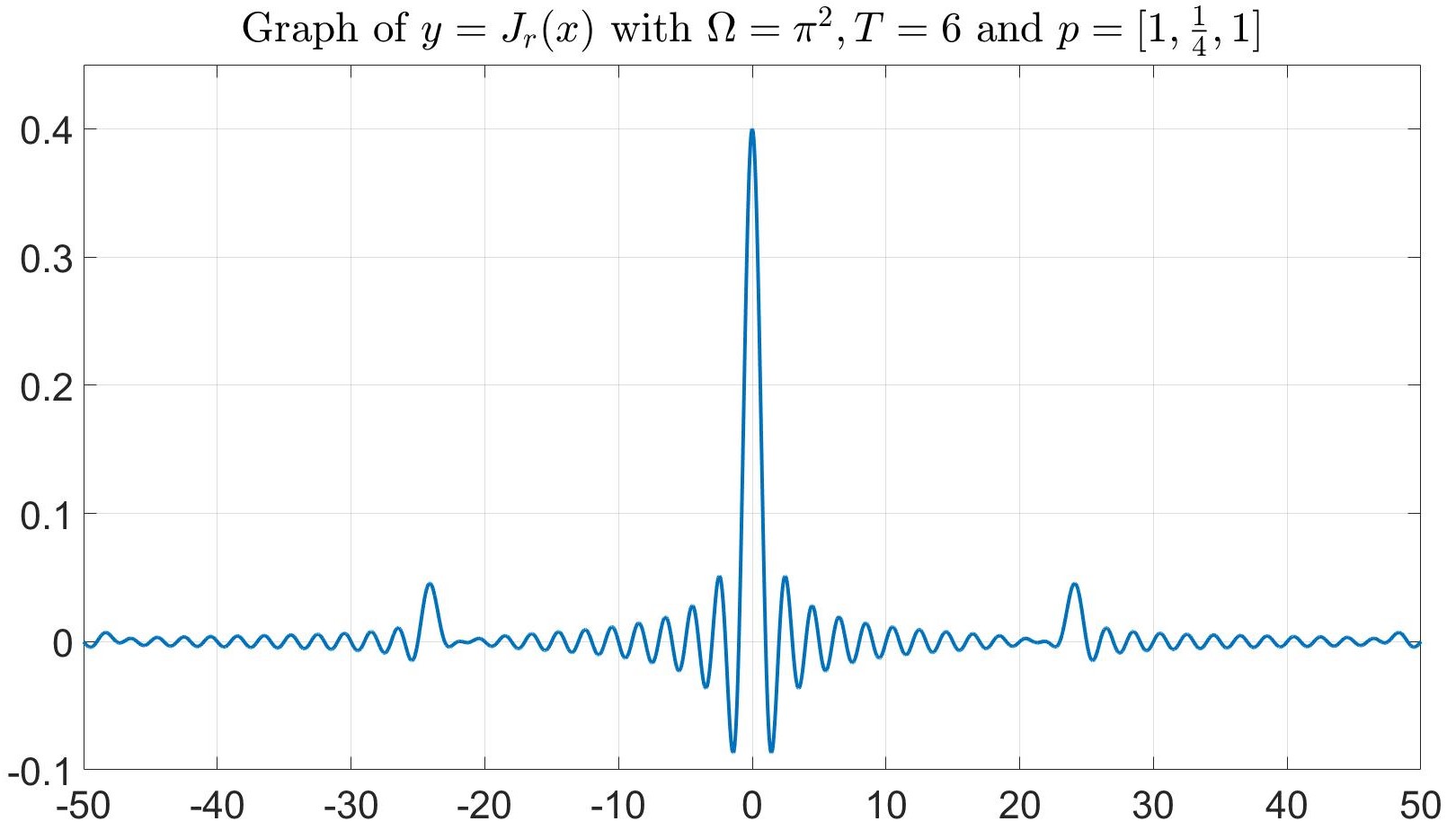
Figure 4.1. Graph of $J_{r}$ when $\Lambda=[0,\pi^{2}]$, $T=6$, $p_{0}=p_{2}=1$ and $p_{1}=\frac{1}{4}$ on the interval $[-50,50]$.

Remark 4.3.

(i) Using the double angle identity for the sine function, one can show that the real part $J_{r}$ of $J$ is given by

(4.8) $$J_{r}(s) =\dfrac{\Omega^{1/2}}{2C\pi}\sum_{m=0}^{\infty}\sum_{l=0}^{m}\left(-\frac{R}{2}\right)^{m}\binom{m}{l}\mathrm{sinc}\left(\Omega^{1/2}(s+(m-2l)\zeta)\right),\quad s\in\mathbb{R}.$$

(ii) In the special case $\Omega^{1/2}=2\pi\zeta l=4\pi q_{1}Tl$ for some $l\in\mathbb{N}$, i.e., if the bandwidth is correlated to the parameters of $p$, then a closed formula for $J$ can be derived in terms of special functions. See [4, Thms. B.0.4, B.0.5].

(iii) In the general case, an alternative expansion for $J_{r}$ can be derived by a change of variables $m-2l\to k$ in (4.8) and a change of the summation order. With

(4.9) $$c_{k} =\frac{\Omega^{1/2}}{2C\pi}\sum_{j=0}^{\infty}\binom{2j+|k|}{j}\left(-\frac{R}{2}\right)^{2j+|k|}$$

(4.10) $$=\frac{\Omega^{1/2}}{2C\pi}\left(-\frac{R}{2}\right)^{|k|}\,_{2}F_{1}\left(\frac{|k|+1}{2},\frac{|k|+2}{2};|k|+1;R^{2}\right),\quad k\in\mathbb{Z},$$

we obtain

$$J_{r}(s)=\sum_{k=-\infty}^{\infty}c_{k}\mathrm{sinc}(\Omega^{1/2}(s-k\zeta)).$$

If $s\in\bigcap_{k\in\mathbb{Z}}\left(k\zeta+\tfrac{\pi}{\Omega^{1/2}}\mathbb{Z}^{*}\right)$, then $J_{r}(s)=0$. In Figure 4.1 we see that for the indicated set of parameters, the zeros of $J_{r}$ are all integers that are not a multiple of $\zeta=2\cdot 2\cdot 6=24$ where peaks with decaying heights occur.

We now derive a complete formula for the reproducing kernel of $PW_{[0,\Omega]}(A_{p})$ with $p$ given in (4.1).

Theorem 4.4.

Let $p_{0},p_{1},p_{2},T>0$, $\Lambda=[0,\Omega]\subset\mathbb{R}_{0}^{+}$ and $p=p_{0}\chi_{(-\infty,-T/2]}+p_{1}\chi_{(-T/2,T/2]}+p_{2}\chi_{[(T/2,\infty)}$. Then the reproducing kernel of $PW_{[0,\Omega]}(A_{p})$ is of the form

$$k_{\Lambda}(x,y)=\sum_{j,l=0}^{2}k_{{jl}}(x,y)\chi_{I_{j}}(x)\chi_{I_{l}}(y),\quad x,y\in\mathbb{R}.$$

The functions $k_{{jl}}$ are

$$k_{00}(x,y) =\tfrac{q_{0}\Omega^{1/2}}{\pi}\mathrm{sinc}(q_{0}\Omega^{1/2}(x-y))+\tfrac{1}{4q_{0}}\left(1-\tfrac{q_{0}^{2}}{q_{1}^{2}}\right)\left(1+\tfrac{q_{1}^{2}}{q_{2}^{2}}\right)J_{r}(q_{0}(x+y+T))$$

$$+\tfrac{1}{8q_{0}}\left(1-\tfrac{q_{0}}{q_{1}}\right)^{2}\left(1-\tfrac{q_{1}^{2}}{q_{2}^{2}}\right)J_{r}(q_{0}(x+y+T)+2q_{1}T)$$

$$+\tfrac{1}{8q_{0}}\left(1+\tfrac{q_{0}}{q_{1}}\right)^{2}\left(1-\tfrac{q_{1}^{2}}{q_{2}^{2}}\right)J_{r}(q_{0}(x+y+T)-2q_{1}T)$$

$$k_{11}(x,y) =\tfrac{1}{2}\left[\tfrac{1}{q_{0}}\left(1+\tfrac{q_{1}^{2}}{q_{2}^{2}}\right)+\tfrac{1}{q_{2}}\left(1+\tfrac{q_{1}^{2}}{q_{0}^{2}}\right)\right]J_{r}(q_{1}(x-y))+\tfrac{1}{2q_{0}}\left(1-\tfrac{q_{1}^{2}}{q_{2}^{2}}\right)J_{r}(q_{1}(x+y-T))$$

$$+\tfrac{1}{2q_{2}}\left(1-\tfrac{q_{1}^{2}}{q_{0}^{2}}\right)J_{r}(q_{1}(x+y+T)),$$

$$k_{22}(x,y) =\tfrac{q_{2}\Omega^{1/2}}{\pi}\mathrm{sinc}(q_{2}\Omega^{1/2}(x-y))+\tfrac{1}{4q_{2}}\left(1+\tfrac{q_{1}^{2}}{q_{0}^{2}}\right)\left(1-\tfrac{q_{2}^{2}}{q_{1}^{2}}\right)J_{r}(q_{2}(x+y-T))$$

$$+\tfrac{1}{8q_{2}}\left(1-\tfrac{q_{1}^{2}}{q_{0}^{2}}\right)\left(1-\tfrac{q_{2}}{q_{1}}\right)^{2}J_{r}(q_{2}(x+y-T)-2q_{1}T)$$

$$+\tfrac{1}{8q_{2}}\left(1-\tfrac{q_{1}^{2}}{q_{0}^{2}}\right)\left(1+\tfrac{q_{2}}{q_{1}}\right)^{2}J_{r}(q_{2}(x+y-T)+2q_{1}T),$$

$$k_{01}(x,y) =k_{10}(y,x)=\tfrac{1}{4q_{0}}\left(1+\tfrac{q_{0}}{q_{1}}\right)\left(1+\tfrac{q_{1}}{q_{2}}\right)^{2}J_{r}(q_{0}(x+\tfrac{T}{2})-q_{1}(y+\tfrac{T}{2}))$$

$$+\tfrac{1}{4q_{0}}\left(1-\tfrac{q_{0}}{q_{1}}\right)\left(1-\tfrac{q_{1}}{q_{2}}\right)^{2}J_{r}(q_{0}(x+\tfrac{T}{2})+q_{1}(y+\tfrac{T}{2}))$$

$$+\tfrac{1}{4q_{0}}\left(1+\tfrac{q_{0}}{q_{1}}\right)\left(1-\tfrac{q_{1}^{2}}{q_{2}^{2}}\right)J_{r}(q_{0}(x+\tfrac{T}{2})+q_{1}(y-\tfrac{3T}{2}))$$

$$+\tfrac{1}{4q_{0}}\left(1-\tfrac{q_{0}}{q_{1}}\right)\left(1-\tfrac{q_{1}^{2}}{q_{2}^{2}}\right)J_{r}(q_{0}(x+\tfrac{T}{2})-q_{1}(y-\tfrac{3T}{2})),$$

$$k_{02}(x,y) =k_{20}(y,x)=\tfrac{1}{2q_{0}}\left(1-\tfrac{q_{0}}{q_{1}}\right)\left(1-\tfrac{q_{1}}{q_{2}}\right)J_{r}(q_{0}(x+\tfrac{T}{2})+q_{1}T-q_{2}(y-\tfrac{T}{2}))$$

$$+\tfrac{1}{2q_{0}}\left(1+\tfrac{q_{0}}{q_{1}}\right)\left(1+\tfrac{q_{1}}{q_{2}}\right)J_{r}(q_{0}(x+\tfrac{T}{2})-q_{1}T-q_{2}(y-\tfrac{T}{2})),$$

$$k_{12}(x,y) =k_{21}(y,x)=\tfrac{1}{4q_{2}}\left(1+\tfrac{q_{1}}{q_{0}}\right)^{2}\left(1+\tfrac{q_{2}}{q_{1}}\right)J_{r}(q_{1}(x-\tfrac{T}{2})-q_{2}(y-\tfrac{T}{2}))$$

$$+\tfrac{1}{4q_{2}}\left(1-\tfrac{q_{1}}{q_{0}}\right)^{2}\left(1-\tfrac{q_{2}}{q_{1}}\right)J_{r}(q_{1}(x-\tfrac{T}{2})+q_{2}(y-\tfrac{T}{2}))$$

$$+\tfrac{1}{4q_{2}}\left(1-\tfrac{q_{1}^{2}}{q_{0}^{2}}\right)\left(1+\tfrac{q_{2}}{q_{1}}\right)J_{r}(q_{1}(x+\tfrac{3T}{2})+q_{2}(y-\tfrac{T}{2}))$$

$$+\tfrac{1}{4q_{2}}\left(1-\tfrac{q_{1}^{2}}{q_{0}^{2}}\right)\left(1-\tfrac{q_{2}}{q_{1}}\right)J_{r}(q_{1}(x+\tfrac{3T}{2})-q_{2}(y-\tfrac{T}{2})).$$

Proof.

Initially we have to consider the following nine pairs of indices:

$$(j,l)\in\{(0,0),(0,1),(0,2),(1,0),(1,1),(1,2),(2,0),(2,1),(2,2)\}.$$

By the symmetry of the reproducing kernel $k_{\Lambda}(x,y)=\overline{k_{\Lambda}(y,x)}$ for all $x,y\in\mathbb{R}$, we see that $(1,0)$ follows from $(0,1)$, $(2,0)$ follows from $(0,2)$, and $(2,1)$ follows from $(1,2)$. Furthermore, since the knots of $p$ are symmetric at the origin, $(2,2)$ follows from $(0,0)$ and $(1,2)$ follows from $(0,1)$ by applying the replacement rule $(x,y,T,q_{0},q_{1},q_{2})\to(y,x,-T,q_{2},q_{1},q_{0})$. Thus, it suffices to take the cases $(j,l)\in\{(0,0),(0,1),(0,2),(1,1)\}.$

Suppose $(j,l)=(0,0)$, i.e., $x,y\leq-\tfrac{T}{2}$. Then upon rearranging the terms, we obtain

(4.11) $$\vartheta(u,x,y) =\frac{1}{q_{0}}\overline{\Phi^{+}(u^{2},x)}\Phi^{+}(u^{2},y)+\frac{1}{q_{n}}\overline{\Phi^{-}(u^{2},x)}\Phi^{-}(u^{2},y),$$

$$=\tfrac{1}{q_{0}}(\overline{a_{0}^{+}(u^{2})}e^{-iq_{0}xu}+\overline{b_{0}^{+}(u^{2})}e^{iq_{0}xu})(a_{0}^{+}(u^{2})e^{iq_{0}yu}+b_{0}^{+}(u^{2})e^{-iq_{0}yu})+\tfrac{1}{q_{2}}e^{iq_{0}xu}e^{-iq_{0}yu}$$

$$=\tfrac{|a_{0}^{+}(u^{2})|^{2}}{q_{0}}e^{-iq_{0}(x-y)u}+\left(\tfrac{1}{q_{2}}+\tfrac{|b_{0}^{+}(u^{2})|^{2}}{q_{0}}\right)e^{iq_{0}(x-y)u}$$

(4.12) $$+\tfrac{1}{q_{0}}\left(a_{0}^{+}(u^{2})\overline{b_{0}^{+}(u^{2})}e^{iq_{0}(x+y)u}+\overline{a_{0}^{+}(u^{2})}b_{0}^{+}(u^{2})e^{-iq_{0}(x+y)u}\right).$$

The above expression simplifies, because $\frac{|b_{0}^{+}(\lambda)|^{2}}{q_{0}^{2}}+\frac{1}{q_{0}q_{n}}=\frac{|a_{0}^{+}(\lambda)|^{2}}{q_{0}^{2}}$ by Corollary 3.5 and by the definition of $\kappa=|a^{+}_{0}(u)|^{2}/q_{0}^{2}$ in (3.25). Upon inserting the connection coefficients $a_{0}^{+}$ and $b_{0}^{+}$ from the proof of Lemma 4.1, we obtain

$$\vartheta(u,x,y) =2q_{0}\kappa(u)\cos(q_{0}(x-y)u)+\tfrac{1}{4q_{0}}\left(1+\tfrac{q_{1}^{2}}{q_{2}^{2}}\right)\left(1-\tfrac{q_{0}^{2}}{q_{1}^{2}}\right)\cos(q_{0}(x+y+T)u)$$

$$+\tfrac{1}{8q_{0}}\left(1-\tfrac{q_{1}^{2}}{q_{2}^{2}}\right)\left(1-\tfrac{q_{0}}{q_{1}}\right)^{2}\cos((q_{0}(x+y+T)+2q_{1}T)u)$$

$$+\tfrac{1}{8q_{0}}\left(1-\tfrac{q_{1}^{2}}{q_{2}^{2}}\right)\left(1+\tfrac{q_{0}}{q_{1}}\right)^{2}\cos((q_{0}(x+y+T)-2q_{1}T)u).$$

Hence,

$$k_{\Lambda}(x,y) =\dfrac{1}{2\pi}\int_{\Lambda^{1/2}}\dfrac{\vartheta(u,x,y)}{\kappa(u)}\,du$$

$$=\tfrac{q_{0}\Omega^{1/2}}{\pi}\mathrm{sinc}(q_{0}\Omega^{1/2}(x-y))+\tfrac{1}{4q_{0}}\left(1+\tfrac{q_{1}^{2}}{q_{2}^{2}}\right)\left(1-\tfrac{q_{0}^{2}}{q_{1}^{2}}\right)J_{r}(q_{0}(x+y+T))$$

$$+\tfrac{1}{8q_{0}}\left(1-\tfrac{q_{1}^{2}}{q_{2}^{2}}\right)\left(1-\tfrac{q_{0}}{q_{1}}\right)^{2}J_{r}(q_{0}(x+y+T)+2q_{1}T)$$

$$+\tfrac{1}{8q_{0}}\left(1-\tfrac{q_{1}^{2}}{q_{2}^{2}}\right)\left(1+\tfrac{q_{0}}{q_{1}}\right)^{2}J_{r}(q_{0}(x+y+T)-2q_{1}T)$$

$$=k_{00}(x,y).$$

The remaining cases are proved in a similar fashion.  

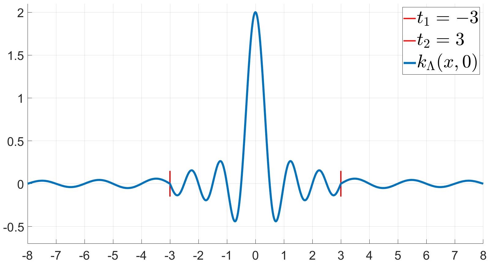
Figure 4.2. Graph of the reproducing kernel $k_{\Lambda}(0,\cdot)$ for the parameters $\Lambda=[0,\pi^{2}],p_{0}=1,p_{1}=\frac{1}{4},p_{2}=1$, $T=6$.

A plot of the reproducing kernel is shown in Figure 4.2. We also note the symmetry of the graph respect to the $y$-axis. Note that the local bandwidth on the interval $[-3,3]$ is $1/\sqrt{p_{1}}=2$ which amounts to two zeros (two oscillations) per unit interval, whereas for $|x|\geq 3$ the local bandwidth is $1/\sqrt{p_{0}}=1/\sqrt{p_{2}}=1$, which amounts to one zero per unit interval. The kernel $k_{\Lambda}(0,\cdot)$ for $PW_{[0,\Omega]}\left(A_{p}\right)$ is the precise analogue of the $\mathrm{sinc}$-kernel $\tfrac{\sin x}{x}$ for the classical Paley-Wiener space.

5. A Density Theorem for Functions of Variable Bandwidth

In this section, we derive necessary density conditions for sampling and interpolation in $PW_{\Lambda}(A_{p})$ with piecewise constant $p$ using a general theory about sampling in reproducing kernel Hilbert spaces from [8].

5.1. Sampling in reproducing kernel Hilbert spaces

We first summarize the definition of density and the necessary density conditions in reproducing kernel Hilbert spaces. For complete details see [8].

For a Borel measure $\mu$ we define the the upper and lower Beurling densities of a separable set $X$ as the quantities

$$D_{\mu}^{+}(X) =\limsup_{r\to\infty}\sup_{x\in\mathbb{R}}\dfrac{\#(X\cap B_{r}(x))}{\mu(B_{r}(x))},$$

$$D_{\mu}^{-}(X) =\liminf_{r\to\infty}\inf_{x\in\mathbb{R}}\dfrac{\#(X\cap B_{r}(x))}{\mu(B_{r}(x))}$$

The relevant measure for sampling in a reproducing kernel Hilbert space with kernel $k$ is $d\mu\left(x\right)=k\left(x,x\right)dx$. The dimension-free Beurling densities $D_{0}^{\pm}(X)$ are defined with respect to the measure $d\mu\left(x\right)=k\left(x,x\right)dx$:

$$D_{0}^{+}(X)=\limsup_{r\to\infty}\sup_{x\in\mathbb{R}}\dfrac{\#(X\cap B_{r}(x))}{\int_{B_{r}(x)}k(x,x)dx},\quad D_{0}^{-}(X)=\liminf_{r\to\infty}\inf_{x\in\mathbb{R}}\dfrac{\#(X\cap B_{r}(x))}{\int_{B_{r}(x)}k(x,x)dx}$$

To derive the desired density theorems in $PW_{\Lambda}(A_{p})$ with piecewise constant $p$, we will use the following special case of [8, Thm. 2.2]. Note the crucial role of the reproducing kernel in the assumptions.

Theorem 5.1.

Assume $k$ is the reproducing kernel for a subspace $\mathcal{H}\subset L^{2}\left(\mathbb{R},dx\right)$ and satisfies the following conditions:

(i) Boundedness of diagonal: There exist constants $C_{1},C_{2}>0$ such that

$$C_{1}\leq k(x,x)\leq C_{2}$$

for all $x\in\mathbb{R}.$

(ii) Weak localization property: For every $\epsilon>0$, there exists $r(\epsilon)>0$ such that

$$\sup_{x\in\mathbb{R}}\int_{\mathbb{R}\setminus B_{r(\epsilon)}(x)}|k(x,y)|^{2}\,dy<\epsilon^{2}.$$

(iii) Homogeneous approximation property: Assume that a subset $X\subseteq\mathbb{R}$ satisfies a Bessel inequality

$$\sum_{x\in X}|f(x)|^{2}\leq C\left\|f\right\|_{\mathcal{H}}^{2}$$

for all $f\in\mathcal{H}$. Then for every $\epsilon>0$ there exists $r(\epsilon)>0$ such that

$$\sup_{y\in\mathbb{R}}\sum_{\underset{|x-y|>r(\epsilon)}{x\in X}}|k(x,y)|^{2}<\epsilon^{2}.$$

Under these assumptions the following density conditions hold in $\mathcal{H}$.

(A) If $X$ is a set of stable sampling for $\mathcal{H}$, then $D_{0}^{-}(X)\geq 1.$

(B) If $X$ is a set of interpolation for $\mathcal{H}$, then $D_{0}^{+}(X)\leq 1.$

Instead of using the measure $k(x,x)\,dx$, this result can be written in terms of any measure $\mu$ equivalent to the Lebesgue measure. For this define the upper and lower averaged traces of $k$ with respect to $\mu$ as

$$\mathrm{tr_{\mu}^{+}}= \limsup_{r\to\infty}\sup_{x\in\mathbb{R}}\dfrac{1}{\mu(B_{r}(x))}\int_{B_{r}(x)}k(y,y)\,dy,$$

$$\mathrm{tr_{\mu}^{-}}= \liminf_{r\to\infty}\inf_{x\in\mathbb{R}}\dfrac{1}{\mu(B_{r}(x))}\int_{B_{r}(x)}k(y,y)\,dy.$$

Then the following reformulation of Theorem 5.1 holds [10, Lemma 6.6].

Lemma 5.2.

Let $d\mu=h\,dx$ be equivalent to the Lebesgue measure. Then $D_{0}^{-}(X)\geq 1$ holds, if and only if $D_{\mu}^{-}\left(X\right)\geq\mathrm{tr_{\mu}^{-}}$. Similarly $D_{0}^{+}\left(X\right)\leq 1$, if and only if $D_{\mu}^{+}\left(X\right)\leq\mathrm{tr_{\mu}^{+}}$.

Proof.

The inequality $D_{0}^{-}(X)\geq 1$ means that for all $\varepsilon>0$ there is an $r_{\epsilon}>0$ such that for all $x\in\mathbb{R}$ and all $r>r_{\varepsilon}$

(5.1) $$\#\left(X\cap B_{r}\left(x\right)\right)\geq\left(1-\varepsilon\right)\int_{B_{r}\left(x\right)}k\left(y,y\right)dy\,,$$

or equivalently,

$$\frac{\#\left(X\cap B_{r}\left(x\right)\right)}{\mu\left(B_{r}\left(x\right)\right)}\geq\left(1-\varepsilon\right)\frac{1}{\mu\left(B_{r}\left(x\right)\right)}\int_{B_{r}\left(x\right)}k\left(y,y\right)dy\,.$$

Written in terms of the Beurling density, this is

$$D_{\mu}^{-}\left(X\right)\geq\liminf_{r\to\infty}\inf_{x\in\mathbb{R}^{d}}\frac{\int_{B_{r}\left(x\right)}k\left(y,y\right)dy}{\mu(B_{r}(x))}=\mathrm{tr}_{\mu}^{-}(k)\,.$$

The converse is obtained by reading the argument backwards.  

5.2. Necessary density conditions in $PW_{[0,\Omega]}\left(A_{p}\right)$

For the Paley-Wiener space $PW_{[0,\Omega]}\left(A_{p}\right)$ we define the positive measure $\mu=\mu_{p}$ by

$$\mu(I)=\mu_{p}(I)=\int_{I}\dfrac{dx}{\sqrt{p(x)}}\,.$$

Since $p$ is positive and bounded away from zero, $\mu_{p}$ is equivalent to Lebesgue measure.

In the case $\mu=\mu_{p}$ we write $D_{p}^{\pm},\operatorname{tr}_{p}^{\pm}$ instead of $D_{\mu_{p}}^{\pm}\left(X\right)$ etc. Our aim is to prove the following theorem for the spectral set $\Lambda$ being an interval.

Theorem 5.3 (Density theorem in $PW_{[0,\Omega]}(A_{p})$).

Let $\Lambda=[0,\Omega]$ and $p$ a piecewise constant function.

1. If $X$ is a set of stable sampling for $PW_{\Lambda}(A_{p})$, then $D_{p}^{-}(X)\geq\frac{|\Lambda^{1/2}|}{\pi}.$

2. If $X$ is a set of interpolation for $PW_{\Lambda}(A_{p})$, then $D_{p}^{+}(X)\leq\frac{|\Lambda^{1/2}|}{\pi}.$

The result is similar to [9, Thms. 6.2, 6.3] but with notable differences in the proofs. In particular, since $p$ is not smooth, not even continuous, we cannot use a Liouville transform to change $A_{p}$ into an equivalent Schrödinger operator and apply scattering theory (as was done in  [9]).

The plan of the proof is to verify the conditions of Theorem 5.1 for the reproducing kernel of $PW(A_{p})$. We will work our way through a series of Lemmas that verify the conditions of Theorem 5.1 and then obtain the value for the averaged trace of the kernel.

5.3. Fine properties of the reproducing kernel of $PW_{[0,\Omega]}\left(A_{p}\right)$

We first verify that the properties of Theorem 5.1 are satisfied for the reproducing kernel of $PW_{[0,\Omega]}\left(A_{p}\right)$.

Lemma 5.4 (Boundedness of the diagonal).

Let $\Lambda\subset\mathbb{R}_{0}^{+}$ be a set of finite measure, $p$ a piecewise constant function and $k_{\Lambda}$ the reproducing kernel for $PW_{\Lambda}(A_{p})$. Then there exist constants $C_{1},C_{2}>0$ such that

$$C_{1}\leq k_{\Lambda}(x,x)\leq C_{2}$$

for all $x\in\mathbb{R}$.

Proof.

The uniform boundedness of $k_{\Lambda}$ (hence the existence of $C_{2}$) follows from the uniform boundedness of the fundamental solutions of $A_{p}$ by Lemma 3.3 and the formula for the reproducing kernel $k_{\Lambda}$ in Theorem 3.8. On the other hand,

$$k_{\Lambda}(x,x) =\dfrac{1}{2\pi}\int_{\Lambda^{1/2}}\dfrac{\frac{1}{q_{0}}|\Phi^{+}(u^{2},x)|^{2}+\frac{1}{q_{n}}|\Phi^{-}(u^{2},x)|^{2}}{\kappa(u)}\,du$$

$$\geq\dfrac{1}{2\pi q_{0}}\int_{\Lambda^{1/2}}\dfrac{|\Phi^{+}(u^{2},x)|^{2}}{\kappa(u)}\,du$$

$$\geq\min_{0\leq j\leq n}\inf_{x\in I_{j}}\dfrac{1}{2\pi q_{0}}\int_{\Lambda^{1/2}}\dfrac{|a_{j}^{+}(u^{2})e^{iq_{j}xu}+b_{j}^{+}(u^{2})e^{-iq_{j}xu}|^{2}}{\kappa(u)}\,du$$

$$\geq\min_{0\leq j\leq n}\dfrac{1}{2\pi q_{0}}\int_{\Lambda^{1/2}}\dfrac{\left||a_{j}^{+}(u^{2})|-|b_{j}^{+}(u^{2})|\right|^{2}}{\kappa(u)}\,du=C_{1}.$$

Since $|a_{j}^{+}(u^{2})|-|b_{j}^{+}(u^{2})|=\frac{q_{j}}{q_{n}}$ by (3.14) and $\kappa$ is bounded, we conclude that $C_{1}>0$.  

Next we show that the kernel $k_{\Lambda}$ exhibits off-diagonal decay. Here we need that $\Lambda$ is an interval.

Lemma 5.5.

Let $\Lambda=[0,\Omega]$ for some $\Omega>0$, $p$ a piecewise constant function and $k_{\Lambda}$ the reproducing kernel for $PW_{[0,\Omega]}(A_{p})$. Then for some constant $C>0$

(5.2) $$|k_{\Lambda}(x,y)|\leq\dfrac{C}{1+|x-y|}\qquad\text{ for all }x,y\in\mathbb{R}\,.$$

Proof.

Let $p$ be a piecewise constant function for some $n\in\mathbb{N}$. Recall the expression (3.38) for the reproducing kernel

$$k_{\Lambda}(x,y)=\sum_{k=1}^{m(x,y)}\alpha_{k}(x,y)J(\beta_{k}(x,y)),\quad m(x,y)\in\mathbb{N},\alpha_{k}(x,y),\beta_{k}(x,y)\in\mathbb{R},1\leq k\leq m(x,y)$$

with $J(s)=\frac{1}{2\pi}\int_{0}^{\Omega^{1/2}}\frac{e^{isu}}{\kappa(u)}\,du$ and $\beta_{k}(x,y)=c_{k}^{(jl)}\pm q_{j}x\pm q_{l}y$ for $x\in I_{j},y\in I_{l}$.

In a first step we show that $J(s)=\mathcal{O}(s^{-1})$ for $\left|s\right|$ large enough. Indeed, as $\kappa$ is (infinitely) differentiable on $(0,\infty)$ with bounded derivatives and $0<\frac{1}{\kappa(u)}\leq q_{0}q_{n}$ for all $u\in(0,\infty)$, integration by parts yields

(5.3) $$J(s) =\dfrac{1}{2\pi is}\left(\dfrac{e^{is\Omega^{1/2}}}{\kappa(\Omega^{1/2})}-\dfrac{1}{\kappa(0^{+})}\right)+\dfrac{1}{2\pi is}\int_{0}^{\Omega^{1/2}}\frac{\kappa^{\prime}(u)}{\kappa(u)^{2}}e^{isu}$$

$$|J(s)| \leq\dfrac{1}{2\pi|s|}\left\{\dfrac{1}{|\kappa(\Omega^{1/2})|}+\dfrac{1}{|\kappa(0^{+})|}+\int_{0}^{\Omega^{1/2}}\dfrac{\left|\kappa^{\prime}(u)\right|}{\kappa(u)^{2}}\,du\right\},$$

where $\kappa(0^{+})=\lim_{u\downarrow 0}\kappa(u)$. Therefore for all $s\neq 0$,

$$|J(s)|\leq\frac{q_{0}q_{n}}{2\pi|s|}\left(2+q_{0}q_{n}\Omega^{1/2}\sup_{0\leq u\leq\Omega^{1/2}}|\kappa^{\prime}(u)|\right).$$

In the second step, we verify that for all $k$ there exist for some $N_{k},r_{k}>0$, such that

(5.4) $$|\beta_{k}(x,y)|\geq{N_{k}}(1+|x-y|)$$

for all $x,y\in\mathbb{R}$ satisfying $|x-y|>r_{k}$. We proceed as follows: let $a>0$ such that the knots $\{t_{k}\}_{k=1}^{n}$ of $p$ are contained in $[-a,a]$. Consider cases where $x$ and $y$ take values on the intervals

$$(-\infty,-a)\subset I_{0},\quad[-a,a]\supset I_{1}\cup\ldots I_{n-1},\quad(a,\infty)\subset I_{n}$$

with $|x-y|$ large.

• Suppose $x$ and $y$ belong to the same unbounded interval, say without loss of generality $x,y<-a$ . Then $\beta_{k}(x,y)=c_{k}\pm q_{0}(x\pm y)$. As $|x\pm y|\geq|x-y|$ we obtain (5.4) for $|x-y|$ sufficiently large, i.e., $|x-y|\geq r_{k}$.

• Likewise the case $|x|\geq a$ and $|y|\leq a$ implies (5.4).

• The remaining case is $x<-a$ and $y>a$, or by symmetry $x>a$ and $y<-a$. Then $|q_{0}x+q_{n}y|$ may be bounded, although $|x-y|\to\infty$, and (5.4) is violated. Here we use the original formulation of $k_{\Lambda}$. We have

  $$\vartheta(u,x,y) =\frac{1}{q_{0}}\overline{\Phi^{+}(u^{2},x)}\Phi^{+}(u^{2},y)+\frac{1}{q_{n}}\overline{\Phi^{-}(u^{2},x)}\Phi^{-}(u^{2},y)$$

  $$=\frac{1}{q_{0}}\Big{(}\overline{a_{0}^{+}(u^{2})}e^{-iq_{0}x}+\overline{b_{0}^{+}(u^{2})}e^{iq_{0}x}\Big{)}e^{iq_{n}yu}+\frac{1}{q_{n}}e^{iq_{0}xu}\Big{(}a_{n}^{-}(u^{2})e^{iq_{n}yu}+b_{n}^{-}(u^{2})e^{-iq_{n}yu}\Big{)}$$

  $$=\Big{(}\frac{\overline{b_{0}^{+}(u^{2})}}{q_{0}}+\frac{a_{n}^{-}(u^{2})}{q_{n}}\Big{)}e^{i(q_{0}x+q_{n}y)u}+\frac{\overline{a_{0}^{+}(u^{2})}}{q_{0}}e^{-i(q_{0}x-q_{n}y)u}+\frac{a_{0}^{+}(u^{2})}{q_{0}}e^{i(q_{0}x-q_{n}y)u}$$

  $$=\frac{\overline{a_{0}^{+}(u^{2})}}{q_{0}}e^{-i(q_{0}x-q_{n}y)u}+\frac{a_{0}^{+}(u^{2})}{q_{0}}e^{i(q_{0}x-q_{n}y)u},$$

  where we have used (3.13) and (3.16) of Lemma 3.4. This implies that there are no exponentials containing $\pm(q_{0}x+q_{n}y)$. Meanwhile, observe that

  $$|q_{0}x-q_{n}y|=q_{n}y-q_{0}x\geq\min(q_{0},q_{n})(y-x)$$

  and (5.4) follows.

To summarize, the decay estimate on $J$ and (5.4) imply that there exists a $C>0$ such that

$$|k_{\Lambda}(x,y)|\leq\frac{C}{1+|x-y|}$$

for all $x,y\in\mathbb{R}$.  

Lemma 5.6 (Weak localization).

Let $\Lambda=[0,\Omega]$ for some $\Omega>0$, $p$ be a piecewise constant function and $k_{\Lambda}$ the reproducing kernel for $PW_{[0,\Omega]}(A_{p})$. Then for every $\epsilon>0$, there exists $r(\epsilon)>0$ such that

(5.5) $$\sup_{x\in\mathbb{R}}\int_{|x-y|>r(\epsilon)}|k_{\Lambda}(x,y)|^{2}\,dy<\epsilon^{2}.$$

Proof.

By Lemma 5.5, we can find $C>0$ such that for all $x,y\in\mathbb{R}$

$$|k_{\Lambda}(x,y)|\leq\dfrac{C}{1+|x-y|}.$$

Let $\epsilon>0$ and take $r(\epsilon)>\max\{b,\frac{4C^{2}}{\epsilon^{2}}-1\}$. Then for a fixed $x\in\mathbb{R}$,

$$\int_{|x-y|>r(\epsilon)}|k_{\Lambda}(x,y)|^{2}\,dy \leq\int_{|x-y|>r(\epsilon)}\dfrac{C^{2}}{(1+|x-y|)^{2}}\,dy=\int_{r(\epsilon)}^{\infty}\dfrac{2C^{2}}{(1+z)^{2}}\,dz$$

$$=\frac{2C^{2}}{1+r(\epsilon)}<\frac{\epsilon^{2}}{2}.$$

Taking the supremum over all $x\in\mathbb{R}$ proves (5.5).  

For the proof of the homogeneous approximation property, we recall that a set $X\subset\mathbb{R}$ is relatively separated if

(5.6) $$\text{rel}(X)=\max_{x\in\mathbb{R}}\#(X\cap[x,x+1])$$

is finite. Lemma 3.7 in [8] implies that if $\{k(x,\cdot):x\in X\}$ is a Bessel sequence for $PW_{\Lambda}\left(\mathbb{R}\right)$ then $X$ is relatively separated.

Lemma 5.7 (Homogeneous approximation property).

Let $\Lambda=[0,\Omega]$ for some $\Omega>0$, $p$ a piecewise constant function and $k_{\Lambda}$ the reproducing kernel for $PW_{[0,\Omega]}(A_{p})$. Suppose $X\subset\mathbb{R}$ such that $\{k_{\Lambda}(x,\cdot):x\in X\}$ is a Bessel sequence in $PW_{[0,\Omega]}(A_{p})$. Then for every $\epsilon>0$, there exists $r(\epsilon)>0$ such that

(5.7) $$\sup_{y\in\mathbb{R}}\sum_{\underset{|x-y|>r(\epsilon)}{x\in X}}|k_{\Lambda}(x,y)|^{2}<\epsilon^{2}.$$

Proof.

Fix $y\in\mathbb{R}$. By Lemma 5.5, there exists $r,C>0$ such that

$$\sum_{\underset{|x-y|>r}{x\in X}}|k_{\Lambda}(x,y)|^{2}\leq\sum_{\underset{|x-y|>r}{x\in X}}\dfrac{C^{2}}{1+|x-y|^{2}}.$$

As $X$ is relatively separated, the right hand side can be made smaller than a given $\epsilon>0$ for $r$ large enough.  

Lemmas 5.6 and 5.7 hold for arbitrary spectral sets $\Lambda$ of finite measure, although the off-diagonal decay of $k_{\Lambda}$ in (5.2) no longer holds. See [4, Lems. C.1.2, C.2.3] for the treatment of the general case.

5.4. The averaged trace of the reproducing kernel

Next we compute the averaged trace of $k$ required for the abstract density theorem (Lemma 5.2). For these arguments $\Lambda$ may be an arbitrary set of finite measure.

To rewrite the diagonal of the reproducing kernel, we define the auxiliary functions

$$h_{j}^{(1)}(u) =\frac{|a_{j}^{+}(u^{2})|^{2}}{q_{0}}+\frac{|a_{j}^{-}(u^{2})|^{2}}{q_{n}}$$

$$h_{j}^{(2)}(u) =\frac{\overline{a_{j}^{+}(u^{2})}b_{j}^{+}(u^{2})}{q_{0}}+\frac{\overline{a_{j}^{-}(u^{2})}b_{j}^{-}(u^{2})}{q_{n}}\,$$

for $0\leq j\leq n$ and $u\in(0,\infty)$.

Lemma 5.8.

Let $\Lambda\subset\mathbb{R}_{0}^{+}$ be of finite measure, $p$ a step function with $n$ jumps and $k_{\Lambda}$ the reproducing kernel for $PW_{\Lambda}(A_{p})$. Then

(5.8) $$k_{\Lambda}(y,y)=\sum_{j=0}^{n}\Big{(}\dfrac{1}{\pi}\int_{\Lambda^{1/2}}\dfrac{h_{j}^{(1)}(u)}{\kappa(u)}\,du+\dfrac{1}{\pi}\emph{Re}\mathcal{F}\big{(}\dfrac{h_{j}^{(2)}}{\kappa}\cdot\chi_{\Lambda^{1/2}}\big{)}(2q_{j}y)\Big{)}\chi_{(t_{j},t_{j+1}]}(y)\,.$$

Proof.

We evaluate the diagonal of $k_{\Lambda}$ using Proposition 3.8. Fix $y\in I_{j}$ for some $0\leq j\leq n$. Using the formula (3.34) for $k_{\Lambda}$, we obtain

$$\vartheta(u,y,y) =\frac{1}{q_{0}}|\Phi^{+}(u^{2},y)|^{2}+\frac{1}{q_{n}}|\Phi^{-}(u^{2},y)|^{2}$$

$$=\frac{1}{q_{0}}|a_{j}^{+}(u^{2})e^{iuq_{j}y}+b_{j}^{+}(u^{2})e^{-iuq_{j}y}|^{2}+\frac{1}{q_{n}}|a_{j}^{-}(u^{2})e^{iuq_{j}y}+b_{j}^{-}(u^{2})e^{-iuq_{j}y}|^{2}$$

$$=\left(\frac{|a_{j}^{+}(u^{2})|^{2}}{q_{0}}+\frac{|b_{j}^{+}(u^{2})|^{2}}{q_{0}}\right)+\left(\frac{|a_{j}^{-}(u^{2})|^{2}}{q_{n}}+\frac{|b_{j}^{-}(u^{2})|^{2}}{q_{n}}\right)$$

$$+2\textrm{Re}\left[\left(\frac{\overline{a_{j}^{+}(u^{2})}b_{j}^{+}(u^{2})}{q_{0}}+\frac{\overline{a_{j}^{-}(u^{2})}b_{j}^{-}(u^{2})}{q_{n}}\right)e^{-2iuq_{j}y}\right]$$

$$=2\left(\frac{|a_{j}^{+}(u^{2})|^{2}}{q_{0}}+\frac{|a_{j}^{-}(u^{2})|^{2}}{q_{n}}\right)+2\textrm{Re}\left[\left(\frac{\overline{a_{j}^{+}(u^{2})}b_{j}^{+}(u^{2})}{q_{0}}+\frac{\overline{a_{j}^{-}(u^{2})}b_{j}^{-}(u^{2})}{q_{n}}\right)e^{-2iuq_{j}y}\right]\,,$$

where in the last identity we have used (3.15). Then

$$k_{\Lambda}(y,y) =\dfrac{1}{2\pi}\int_{\Lambda^{1/2}}\dfrac{\vartheta(u,y,y)}{\kappa(u)}\,du$$

$$=\dfrac{1}{\pi}\int_{\Lambda^{1/2}}\dfrac{h_{j}^{(1)}(u)}{\kappa(u)}\,du+\dfrac{1}{\pi}\int_{\Lambda^{1/2}}\dfrac{\textrm{Re}(h_{j}^{(2)}(u)e^{-2iq_{j}yu})}{\kappa(u)}\,du$$

$$=\dfrac{1}{\pi}\int_{\Lambda^{1/2}}\dfrac{h_{j}^{(1)}(u)}{\kappa(u)}\,du+\dfrac{1}{\pi}\textrm{Re}\,\mathcal{F}\left(\dfrac{h_{j}^{(2)}}{\kappa}\cdot\chi_{\Lambda^{1/2}}\right)(2q_{j}y)$$

as claimed.  

Note that the first term $\int h^{(1)}_{j}$ depends only on the interval $I_{j}$ , but not on $y\in I_{j}$.

In the following theorem we compute the averaged trace of the kernel $k$. We recall that the notation $f\lesssim g$ means that there exists $C\geq 0$ such that $f\leq Cg$.

Theorem 5.9.

Let $\Lambda\subset\mathbb{R}_{0}^{+}$ be of finite measure, $p$ a piecewise constant function and $k_{\Lambda}$ the reproducing kernel of $PW_{\Lambda}(A_{p})$. Suppose $I$ is a large interval such that $I\not\subset[t_{1},t_{n}]$. Then

$$\left|\dfrac{1}{\mu_{p}(I)}\int_{I}k_{\Lambda}(y,y)\,dy-\dfrac{|\Lambda^{1/2}|}{\pi}\right|\lesssim\mu_{p}(I)^{-1/2}\,.$$

In particular,

$$\emph{tr}^{-}=\liminf_{r\to\infty}\inf_{x\in\mathbb{R}}\dfrac{1}{\mu_{p}(B_{r}(x))}\int_{B_{r}(x)}k_{\Lambda}(y,y)\,dy=\frac{|\Lambda^{1/2}|}{\pi}\,,$$

and likewise $\emph{tr}^{+}=\frac{|\Lambda^{1/2}|}{\pi}$.

Proof.

Let $p$ be a piecewise constant function with $n$ jumps at $\{t_{k}\}_{k=1}^{n}$. We may assume that the interval $I=[\alpha,\beta]\supseteq[t_{1},t_{n}]$. The two other cases are easier to handle. Since $\frac{1}{\sqrt{p(x)}}\chi_{(t_{j},t_{j+1}]}(x)=q_{j}$ for $x\in(t_{j},t_{j+1}]$, we obtain

(5.9) $$\mu_{p}(I) \int_{\alpha}^{\beta}\frac{1}{\sqrt{p(x)}}\,dx=\left[q_{0}(t_{1}-\alpha)+q_{n}(\beta-t_{n})\right]+\sum_{j=1}^{n-1}q_{j}(t_{j+1}-t_{j})\,,$$

and $\mu_{p}(I)\geq(\beta-\alpha)\min_{j}q_{j}$. We first observe that

$$\dfrac{1}{\mu_{p}(I)}\int_{I}k_{\Lambda}(y,y)\,dy=\dfrac{1}{\mu_{p}(I)}\int_{I\setminus[t_{1},t_{n}]}k_{\Lambda}(y,y)\,dy+\dfrac{1}{\mu_{p}(I)}\int_{[t_{1},t_{n}]}k_{\Lambda}(y,y)\,dy\,.$$

Since the second term in this some is of the form $C\mu_{p}(I)^{-1}$ we can focus on the first term. We use the representation of the diagonal of $k_{\Lambda}$ obtained in Lemma 5.8 and consider first the expression

$$T_{1}=\dfrac{1}{\mu_{p}(I)\pi}\Big{(}\int_{\alpha{}_{\alpha}}^{t_{1}}\int_{\Lambda^{1/2}}\dfrac{h_{0}^{(1)}(u)}{\kappa(u)}\,du\,dy+\int_{t_{n}}^{\beta}\int_{\Lambda^{1/2}}\dfrac{h_{0}^{(1)}(u)}{\kappa(u)}\,du\,dy\Big{)}\,.$$

Using the initial conditions $a_{0}^{-}=b_{n}^{+}=0$, $a_{n}^{+}=b_{0}^{-}=1$ and the definition of $\kappa$ in (3.25), we obtain

$$h_{0}^{(1)}(u)=\frac{|a_{0}^{+}(u^{2})|^{2}}{q_{0}}=q_{0}\kappa(u),\quad h_{n}^{(1)}(u)=\frac{|b_{n}^{-}(u^{2})|^{2}}{q_{n}}=q_{n}\kappa(u)\,,$$

and consequently

$$T_{1} =\dfrac{|\Lambda^{1/2}|}{\mu_{p}(I)\pi}\left(q_{0}(t_{1}-\alpha)+q_{n}(\beta-t_{n})\right)$$

$$=\dfrac{|\Lambda^{1/2}|}{\mu_{p}(I)\pi}\Big{(}\mu_{p}(I)-\sum_{j=1}^{n-1}q_{j}(t_{j+1}-t_{j})\Big{)}=\dfrac{|\Lambda^{1/2}|}{\pi}+\mathcal{O}\big{(}\dfrac{1}{\mu_{p}(I)}\big{)}.$$

This leads to the estimate

(5.10) $$\left|T_{1}-\dfrac{|\Lambda^{1/2}|}{\pi}\right|\lesssim\mu_{p}(I)^{-1}\lesssim\mu_{p}(I)^{-1/2}.$$

For the second term, we make a similar computation. Let

$$T_{2} =\dfrac{1}{\mu_{p}(I)\pi}\int_{I\setminus[t_{1},t_{n}]}\textrm{Re}\mathcal{F}\Big{(}\dfrac{h_{j}^{(2)}}{\kappa}\cdot\chi_{\Lambda^{1/2}}\Big{)}(2q_{j}y)\,dy$$

$$=\dfrac{1}{\mu_{p}(I)\pi}\textrm{Re}\left(\int_{\alpha}^{t_{1}}\int_{\Lambda^{1/2}}\dfrac{h_{0}^{(2)}(u)e^{-2iq_{0}yu}}{\kappa(u)}\,du\,dy+\int_{t_{n}}^{\beta}\int_{\Lambda^{1/2}}\dfrac{h_{n}^{(2)}(u)e^{-2iq_{n}yu}}{\kappa(u)}\,du\,dy\right)\,.$$

Interchanging the order of integration and evaluating the integral over $y$ first, we have

$$T_{2} =\dfrac{1}{\mu_{p}(I)\pi}\textrm{Re}\int_{\Lambda^{1/2}}\dfrac{h_{0}^{(2)}(u)e^{-2iq_{0}(t_{1}+\alpha)u}}{\kappa(u)}\cdot\dfrac{\sin(q_{0}(t_{1}-\alpha)u)}{q_{0}u}\,du$$

$$+\dfrac{1}{\mu_{p}(I)\pi}\textrm{Re}\int_{\Lambda^{1/2}}\dfrac{h_{n}^{(2)}(u)e^{-2iq_{n}(\beta+t_{n})u}}{\kappa(u)}\cdot\dfrac{\sin(q_{n}(\beta-t_{n})u)}{q_{n}u}\,du.$$

With the Cauchy-Schwartz inequality, this can be estimated as

$$\left|T_{2}\right| \leq\dfrac{1}{\mu_{p}(I)\pi}\left(C_{0}\left(\int_{\Lambda^{1/2}}\dfrac{\sin^{2}(q_{0}(t_{1}-\alpha)u)}{(q_{0}u)^{2}}du\right)^{1/2}+C_{n}\left(\int_{\Lambda^{1/2}}\dfrac{\sin^{2}(q_{n}(\beta-t_{n})u)}{(q_{n}u)^{2}}du\right)^{1/2}\right)$$

$$=\dfrac{C_{0}}{\mu_{p}(I)\pi}\left(\frac{t_{1}-\alpha}{q_{0}}\int_{q_{0}(t_{1}-\alpha)\Lambda^{1/2}}\!\mathrm{sinc}^{2}\omega\,d\omega\right)^{1/2}+\dfrac{C_{n}}{\mu_{p}(I)\pi}\left(\frac{\beta-t_{n}}{q_{n}}\int_{q_{n}(\beta-t_{n})\Lambda^{1/2}}\!\mathrm{sinc}^{2}\omega\,d\omega\right)^{1/2}$$

$$\leq\dfrac{C}{\mu_{p}(I)\pi}\mu_{p}(I)^{1/2}\leq C^{\prime}\mu_{p}(I)^{-1/2}\,.$$

Putting these estimates together we obtain

(5.11) $$\left|\dfrac{1}{\mu_{p}(I)}\int_{I}k_{\Lambda}(y,y)\,dy-\dfrac{|\Lambda^{1/2}|}{\pi}\right|=\left|T_{1}+T_{2}-\dfrac{|\Lambda^{1/2}|}{\pi}\right|\leq C\mu_{p}(I)^{-1/2}\,.$$

 

5.5. Proof of Theorem 5.3

Proof.

Theorem 5.3 now follows from the general density theorem as stated in Theorem 5.1. In Lemmas 5.4 — 5.7 we have verified that the conditions on the reproducing kernel are satisfied, and in Theorem 5.9 we have computed the critical density given by the averaged trace of the kernel.  

Remark.

We finish by mentioning that the assumptions on the spectral set $\Lambda$ can be weakened and Theorem 5.3 remains true, when $\Lambda$ is just a set of finite measure.

If the spectral set is not an interval $[0,\Omega]$, then Proposition 5.5 no longer holds, and therefore the proofs of Lemmas 5.6 and 5.7 do not work for general spectral sets. Nevertheless the conclusions of 5.6 and 5.7 still hold whenever $\Lambda$ has finite measure. The proofs are more delicate and the interested reader is referred to [4].

References

- [1] R. Aceska and H. Feichtinger. Functions of variable bandwidth via time-frequency analysis tools. Journal of Mathematical Analysis and Applications, 382(1):275 – 289, 2011.
- [2] R. Aceska and H. Feichtinger. Reproducing kernels and variable bandwidth. Journal of Function Spaces and Applications, 2012, 2012.
- [3] N. N. Brueller, N. Peterfreund, and M. Porat. Non-stationary signals: optimal sampling and instantaneous bandwidth estimation. In Proceedings of the IEEE-SP International Symposium on Time-Frequency and Time-Scale Analysis (Cat. No.98TH8380), pages 113–115, Oct 1998.
- [4] M. J. Celiz. Spaces of functions of variable bandwidth parametrized by piecewise constant functions. PhD thesis, Wien, 2022. Universität Wien, Dissertation.
- [5] J. Clark, M. Palmer, and P. Lawrence. A transformation method for the reconstruction of functions from nonuniformly spaced samples. IEEE Transactions on Acoustics, Speech, and Signal Processing, 33(5):1151–1165, October 1985.
- [6] N. Dunford and J. T. Schwartz. Linear operators. Part II: Spectral theory. Self adjoint operators in Hilbert space. With the assistance of William G. Bade and Robert G. Bartle. Interscience Publishers John Wiley & Sons New York-London, 1963.
- [7] C. Fefferman. The Bergman kernel and biholomorphic mappings of pseudoconvex domains. Invent. Math., 26:1–65, 1974.
- [8] H. Führ, K. Gröchenig, A. Haimi, A. Klotz, and J. L. Romero. Density of sampling and interpolation in reproducing kernel Hilbert spaces. J. Lond. Math. Soc. (2), 96(3):663–686, 2017.
- [9] K. Gröchenig and A. Klotz. What is variable bandwidth? Comm. Pure Appl. Math., 70(11):2039–2083, 2017.
- [10] K. Gröchenig and A. Klotz. Necessary density conditions for sampling and interpolation in spectral subspaces of elliptic differential operators. Anal. PDE, 2023. to appear.
- [11] K. Horiuchi. Sampling principle for continuous signals with time-varying bands. Information and Control, 13:53–61, 1968.
- [12] I.Pesenson and A. Zayed. Paley–Wiener subspace of vectors in a Hilbert space with applications to integral transforms. Journal of Mathematical Analysis and Applications, 353(2):566 – 582, 2009.
- [13] H. J. Landau. Necessary density conditions for sampling and interpolation of certain entire functions. Acta Math., 117:37–52, 1967.
- [14] R. Martin and A. Kempf. Function spaces obeying a time-varying bandlimit. Journal of Mathematical Analysis and Applications, 458(2):1597 – 1638, 2018.
- [15] I. Pesenson. Sampling of band-limited vectors. Journal of Fourier Analysis and Applications, 7(1):93–100, Jan 2001.
- [16] M. Schmied, R. Sims, and G. Teschl. On the absolutely continuous spectrum of Sturm-Liouville operators with applications to radial quantum trees. Oper. Matrices, 2(3):417–434, 2008.
- [17] G. Teschl. Mathematical Methods in Quantum Mechanics. Graduate Studies in Mathematics. American Mathematical Society, 2014.
- [18] V. K. Tuan and A. I. Zayed. Paley-Wiener-type theorems for a class of integral transforms. J. Math. Anal. Appl., 266(1):200–226, 2002.
- [19] D. Wei and A. V. Oppenheim. Sampling based on local bandwidth. In 2007 Conference Record of the Forty-First Asilomar Conference on Signals, Systems and Computers, pages 1103–1107, Nov 2007.
- [20] J. Weidmann. Spectral theory of ordinary differential operators. Lecture notes in mathematics. Springer, 1987.
- [21] J. Weidmann. Lineare Operatoren in Hilberträumen: Teil 2 Anwendungen. Mathematische Leitfäden. Vieweg+Teubner Verlag, 2003.