A New Approach for Designing Well-Balanced Schemes for the Shallow Water Equations: A Combination of Conservative and Primitive Formulations

Abstract

In this paper, we introduce a novel approach for constructing robust, fully well-balanced numerical methods for the one-dimensional Saint-Venant system, both with and without the Manning friction term. Inspired by the method presented in [R. Abgrall, Commun. Appl. Math. Comput. 5(2023), pp. 370-402], we first combine the conservative and primitive formulations of the studied hyperbolic system in a natural way. The solution is globally continuous and described by a combination of point and average values. The point and average values will then be evolved by two different forms of PDEs. We show how to deal with both the conservative and primitive forms of PDEs in a well-balanced manner. The developed schemes are capable of exactly preserving both the still-water and moving-water equilibria. We demonstrate the behavior of the proposed new scheme on several challenging examples.

Key words: Shallow water equations, Well-balanced schemes, Steady states, MOOD paradigm.

AMS subject classification: 76M12, 65M08, 65M99, 35L40, 35L65

1 Introduction

The paper focus on the one-dimensional (1-D) Saint-Venant system of shallow water equations with non-flat bottom topography and Manning friction term, which is widely used to model the water flows in rivers, canals, lakes, reservoirs, and coastal areas. The studied system reads as

$$\left\{\begin{aligned} &h_{t}+q_{x}=0,\\ &q_{t}+\left(hu^{2}+\frac{g}{2}h^{2}\right)_{x}=-ghZ_{x}-\frac{gn^{2}}{h^{\frac{7}{3}}}|q|q,\end{aligned}\right.$$ (1.1)

where $g$ is the constant acceleration due to gravity, $x$ is the spatial variable, and $t$ is the time. $h(x,t)$ is the water depth, $u(x,t)$ is the velocity, and $q(x,t):=h(x,t)u(x,t)$ is the discharge. $Z(x)$ is the bottom elevation and $n$ is the Manning coefficient.

The system (1.1) is a hyperbolic system of balance laws. Developing robust and accurate numerical methods for such a system is a challenging task as this nonlinear hyperbolic system admits both smooth and nonsmooth solutions. In addition, a good numerical scheme should be able to accurately respect a delicate balance between the flux and source term in (1.1). In particular, one is interested in developing well-balanced (WB) numerical schemes that are capable of exactly preserving (some of) steady states. If a stable but non-well-balanced scheme is used, then the numerical errors may trigger the appearance of artificial waves of magnitude larger than the size of the waves to be captured. In order to ameliorate this situation, one can do mesh refinement so that the numerical errors will be controlled by the truncation errors. However, such mesh refinement may be too computationally expensive or even unaffordable in practical applications. Therefore, one needs to develop WB schemes.

Steady states are of great practical importance since they minimize, if they are stable, the energy, and many physically relevant solutions of (1.1) are, in fact, small perturbations of these steady states. The smooth steady-state solutions of (1.1) satisfy the following time-independent system:

$$\left\{\begin{aligned} &q_{x}=0,\\ &\big{(}hu^{2}+\frac{g}{2}h^{2}\big{)}_{x}=-ghZ_{x}-\frac{gn^{2}}{h^{\frac{7}{3}}}|q|q,\end{aligned}\right.$$ (1.2)

which can be integrated to obtain

$$q\equiv\widehat{q}={\rm Const},\quad{E}:=\frac{u^{2}}{2}+g(h+Z)+Q\equiv\widehat{E}={\rm Const},$$ (1.3)

where

$$Q=\int\limits_{\widehat{x}}^{x}\frac{gn^{2}}{h^{\frac{10}{3}}}|q|q\,{\rm d}\xi$$ (1.4)

is a global quantity with $\widehat{x}$ being an arbitrary number. In the case when $u\equiv 0$, the steady states (1.3) reduce to a particular class of steady states—still-water equilibria (“lake at rest”):

$$u\equiv 0,\quad w:=h+Z\equiv{\rm Const},$$ (1.5)

where $w$ is the water surface. In fact, still-water steady state (1.5) is a special case of the general moving-water steady state (1.3). If the bottom friction is neglected, that is, if $n=0$, the general smooth moving-water equilibria are given by

$$q\equiv\widehat{q}={\rm Const},\quad E:=\frac{u^{2}}{2}+g(h+Z)\equiv\widehat{E}={\rm Const}.$$ (1.6)

In the past decades, many WB methods for the system (1.1) have been developed. Some of them are capable of preserving still-water steady states (1.5) only (see, e.g., [3, 5, 6, 22, 26, 30, 37, 38, 33, 23]), while others can preserve moving-water equilibria as well (see, e.g., [10, 13, 14, 17, 18, 36, 41, 15, 35, 8]). One may notice that it is significantly more difficult to obtain WB schemes for moving-water equilibria, since a special way to recover the moving water equilibrium and a WB quadrature rule of the source term is essential to design such schemes. The authors in [10, 13, 15, 14, 17, 36, 18, 8, 40] first define a transformation between the conservative variables $(h,q)^{\top}$ and the equilibrium variables $(q,E)^{\top}$. Then, the polynomial reconstruction will be performed on the equilibrium variables and one can obtain the one-sided cell boundary point values of the equilibrium variables. Next, the one-sided cell boundary point values of the conservative variables can be recovered from the point values of the equilibrium variables. At this stage, one usually has to solve nonlinear equations, as it can be clearly seen from (1.3) or (1.6) that the transformation is nonlinear. In order to recover the point values of conservative variables from the nonlinear transformation and reconstructed point values of equilibrium variables, a nontrivial root-finding mechanism should be carefully developed. In addition, the solution of nonlinear equation is usually nonunique, one has to design a proper principle to single out the unique physical-relevant solution. Finally, WB evaluations of the numerical flux and approximation of the source term are computed using the obtained reconstructed point values of conservative variables.

Very recently, the author in [1] proposed a new class of schemes that can combine several writings of the same hyperbolic problem and showed how to deal with both the conservative and non-conservative forms in a natural way. In these schemes, the solution is globally continuous and described by a combination of point values and average values. The author demonstrated that one can recover the conservation property from how the average is updated and has more flexibility to deal directly with the primitive form of the system. This new class of schemes is proved to satisfy a Lax-Wendroff-like theorem and also showed numerically that the convergence to the correct weak solution.

In this paper, inspired by the method introduced in [1], we develop a novel way for designing WB schemes. In addition to the conservative system (1.1), we simultaneously study the following primitive formulation:

$$\left\{\begin{aligned} &h_{t}+hu_{x}+uh_{x}=0,\\ &u_{t}+uu_{x}+g(h+Z)_{x}=-\frac{gn^{2}}{h^{\frac{4}{3}}}|u|u,\\ \end{aligned}\right.$$ (1.7)

which can be rewritten as

$$\left\{\begin{aligned} &h_{t}+q_{x}=0,\\ &u_{t}+E_{x}=0,\\ \end{aligned}\right.$$ (1.8)

by employing the definition of equilibrium variables $q$ and $E$ in (1.3). Since we have more flexibility to work on the primitive form, unlike most of the existing works mentioned above, this new class of WB schemes does not require a nontrivial root-finding mechanism. More precisely, we design a WB finite-volume method for system (1.1) to evolve the cell averages of conservative variables $(h,q)^{\top}$ and simultaneously propose a WB residual distribution (RD) method for system (1.8) to evolve the point values of primitive variables $(h,u)^{\top}$. Given the average and point values of conservative variables (the point values of conservative variables can be obtained from the point values from the primitive variables), we can apply a third-order parabolic interpolant on the conservative variables and then compute the point values of conservative variables at the cell center. Having these point values of conservative variables allows us to compute the point values of equilibrium variables at the cell center and cell interfaces. Next, we do the spatial discretizations on the equilibrium variables, which helps to ensure the WB property. It follows from (1.3) that the approximations of spatial derivatives appear in (1.8) will vanish when the solution is at the steady sate. Unlike many existing methods, at this stage, we do not relay on any special root-finding mechanism. Instead, we compute the fluctuation of the system (1.8) directly based on the equilibrium variables, and split the residual onto the nodes through an upwind consideration. For numerically solving (1.1), we simply compute the flux using the point values of primitive variables at the cell interfaces and a WB approximation of source term is given using the values of equilibrium variables. In addition to the WB property, the developed schemes are positivity-preserving. This attributes to the fact that we have applied a MOOD paradigm from [20, 39] equipped with a first-order scheme that has a Local Lax-Friedrichs’ flavour to the solvers of (1.1) and (1.8).

The rest of the paper is organized as follows. In 2, we introduce the new WB positive-preserving schemes for the conservative formulation (1.1) and the primitive formulation (1.8). In 3, we present the numerical results, which demonstrate the WB property, positivity-preserving property, high resolution, and robustness of the proposed schemes. Finally, in 4, we give some concluding remarks and comments on the future development and applications of the proposed WB schemes.

2 Schemes

In this section, we describe the third-order semi-discrete numerical schemes for the 1-D Saint-Venant system (1.1) and its primitve version (1.8). To this end, we first rewrite (1.1) in a vector form as

$$\bm{U}_{t}+\bm{F}(\bm{U})_{x}=\bm{S}(\bm{U}),\quad\bm{U}=(h,q)^{\top},$$ (2.1)

where $\bm{U}\in\mathbb{R}^{d}$ and

$$\bm{F}(\bm{U})=\begin{pmatrix}q\\ hu^{2}+\frac{g}{2}h^{2}\end{pmatrix},\quad\bm{S}(\bm{U})=\begin{pmatrix}0\\ -ghZ_{x}-hQ_{x}\end{pmatrix}.$$ (2.2)

Simultaneously, we also rewrite (1.8) in the following vector form:

$$\bm{V}_{t}+\frac{\partial\bm{E}}{\partial x}=\bm{0},\quad\bm{V}=(h,u)^{\top},\quad\bm{E}=(q,E)^{\top},$$ (2.3)

where $\bm{V}=\Psi(\bm{U})$ with

$$\Psi:\mathcal{D}_{\bm{U}}\rightarrow\mathcal{D}_{\bm{V}},~{}\mathcal{D}_{\bm{U}}=\{\bm{U}=(h,q)^{\top}\in\mathbb{R}^{2}:h\geq 0\},~{}\mathcal{D}_{\bm{V}}=\{\bm{V}=(h,u)^{\top}\in\mathbb{R}^{2}:h\geq 0\}.$$

We divide the computational domain into a set of uniform (for simplicity of presentation) cells $K_{j+\frac{1}{2}}:=[x_{j},x_{j+1}]$ of size $\Delta x=x_{j+1}-x_{j}$, which are centered at $x_{j+\frac{1}{2}}=(x_{j}+x_{j+1})/2$. We assume that at a certain time level $t$, the numerical solution of (2.1)–(2.2), realized in terms of its cell average $\,\hbox{\vbox{\hrule height=0.5pt\kern 1.72218pt\hbox{\kern-0.50003pt$\bm{U}$\kern 0.0pt}}}_{j+\frac{1}{2}}(t)\approx\frac{1}{\Delta x}\int_{K_{j+\frac{1}{2}}}\bm{U}(x,t)\,{\rm d}x$, is available. We denote the numerical solutions of (2.3) by $\bm{V}_{j}(t)\approx\bm{V}(x_{j},t)$, which are also known at time $t$. Following the method introduced in [1], we evolve the cell averages $\hbox{\vbox{\hrule height=0.5pt\kern 1.72218pt\hbox{\kern-0.50003pt$\bm{U}$\kern 0.0pt}}}_{j+\frac{1}{2}}$ in time by solving the following system of time-dependent ODEs:

$$\frac{\rm d}{{\rm d}t}\,\hbox{\vbox{\hrule height=0.5pt\kern 1.72218pt\hbox{\kern-0.50003pt$\bm{U}$\kern 0.0pt}}}_{j+\frac{1}{2}}=-\frac{\bm{\mathcal{F}}_{j+1}-\bm{\mathcal{F}}_{j}}{\Delta x}+\hbox{\vbox{\hrule height=0.5pt\kern 1.72218pt\hbox{\kern-0.50003pt$\bm{S}$\kern 0.0pt}}}_{j+\frac{1}{2}},$$ (2.4)

where

$$\bm{\mathcal{F}}_{j}=\bm{F}(\bm{U}_{j})\stackrel{{\scriptstyle(\ref{2.2})}}{{=}}\begin{pmatrix}q_{j}\\ h_{j}u_{j}^{2}+\frac{g}{2}h_{j}^{2}\end{pmatrix}$$ (2.5)

and

$$\hbox{\vbox{\hrule height=0.5pt\kern 1.72218pt\hbox{\kern-0.50003pt$\bm{S}$\kern 0.0pt}}}_{j+\frac{1}{2}}:\approx\frac{1}{\Delta x}\int\limits_{K_{j+\frac{1}{2}}}{\bm{S}}(\bm{U}(x,t)){\rm d}x$$ (2.6)

is an approximation of the cell average of source term. At the same time, the point values $\bm{V}_{j}$ are also evolved by solving a system of time-dependent ODEs given by

$$\frac{\rm d}{{\rm d}t}\,{\bm{V}}_{j}=-(\overleftarrow{\Phi}_{j+\frac{1}{2}}^{\bm{V}}+\overrightarrow{\Phi}_{j-\frac{1}{2}}^{\bm{V}}),$$ (2.7)

where $\overleftarrow{\Phi}_{j+\frac{1}{2}}^{\bm{V}}+\overrightarrow{\Phi}_{j-\frac{1}{2}}^{\bm{V}}$ is a consistent approximation of $\frac{\partial\bm{E}}{\partial x}(x_{j})$. Notice that all of the indexed quantities in (2.4)–(2.6), and (2.7) are time-dependent, but from here on, we omit this dependence for the sake of brevity.

Given the point value $\bm{U}_{j}=\Psi(\bm{V}_{j})$ and the cell average $\hbox{\vbox{\hrule height=0.5pt\kern 1.72218pt\hbox{\kern-0.50003pt$\bm{U}$\kern 0.0pt}}}_{j+\frac{1}{2}}$, we begin with computing the point value $\bm{U}_{j+\frac{1}{2}}$ at the cell center, which is given by

$$\bm{U}_{j+\frac{1}{2}}:=\widetilde{\bm{U}}(x_{j+\frac{1}{2}})=\frac{3}{2}\,\hbox{\vbox{\hrule height=0.5pt\kern 1.72218pt\hbox{\kern-0.50003pt$\bm{U}$\kern 0.0pt}}}_{j+\frac{1}{2}}-\frac{1}{4}(\bm{U}_{j}+\bm{U}_{j+1})$$ (2.8)

with $\widetilde{\bm{U}}(x)$ being a third-order parabolic interpolant of $\bm{U}$ defined on $K_{j+\frac{1}{2}}$, that can be found in (A.1) from Appendix A.

We proceed with computing the point values of $Q$. To this end, we rewrite the global quantity $Q$ defined in (1.4) in a recursive way and approximate the yield integration part by the Simpson’s rule. Namely, we take

$$Q_{j+\frac{1}{2}} =Q_{j}+\int\limits_{x_{j}}^{x_{{j+\frac{1}{2}}}}\frac{gn^{2}}{h^{\frac{10}{3}}}|q|q\,{\rm d}x$$ (2.9)

$$\approx Q_{j}+\frac{gn^{2}\Delta x}{12}\left(\frac{|q_{j}|q_{j}}{(h_{j})^{10/3}}+\frac{|q_{j+\frac{1}{2}}|q_{j+\frac{1}{2}}}{(h_{j+\frac{1}{2}})^{10/3}}+4\frac{|q_{j+\frac{1}{4}}|q_{j+\frac{1}{4}}}{(h_{j+\frac{1}{4}})^{10/3}}\right),$$

$$Q_{j+1} =Q_{j}+\int\limits_{x_{j}}^{x_{j+1}}\frac{gn^{2}}{h^{\frac{10}{3}}}|q|q\,{\rm d}x$$

$$\approx Q_{j}+\frac{gn^{2}\Delta x}{6}\left(\frac{|q_{j}|q_{j}}{(h_{j})^{10/3}}+\frac{|q_{j+1}|q_{j+1}}{(h_{j+1})^{10/3}}+4\frac{|q_{j+\frac{1}{2}}|q_{j+\frac{1}{2}}}{(h_{j+\frac{1}{2}})^{10/3}}\right),$$

where $\bm{U}_{j+\frac{1}{2}}$ is given in (2.8), $\bm{U}_{j+\frac{1}{4}}$ can be computed from (A.1):

$$\bm{U}_{j+\frac{1}{4}}=\frac{3}{16}\bm{U}_{j}+\frac{18}{16}\hbox{\vbox{\hrule height=0.5pt\kern 1.72218pt\hbox{\kern-0.50003pt$\bm{U}$\kern 0.0pt}}}_{j+\frac{1}{2}}-\frac{5}{16}\bm{U}_{j+1},$$ (2.10)

and $Q_{1}=0$ as we simply take $\widehat{x}=x_{1}$ in (1.4).

We then compute the point values $\bm{E}_{j}=(q_{j},E_{j})^{\top}$ and ${\bm{E}}_{j+\frac{1}{2}}=(q_{j+\frac{1}{2}},E_{j+\frac{1}{2}})^{\top}$ for all $j$ as follows:

$$q_{j}:=h_{j}u_{j},\quad E_{j}=\frac{u_{j}^{2}}{2}+g(h_{j}+Z_{j})+Q_{j},$$ (2.11)

$$E_{j+\frac{1}{2}}=\frac{u_{j+\frac{1}{2}}^{2}}{2}+g(h_{j+\frac{1}{2}}+Z_{j+\frac{1}{2}})+Q_{j+\frac{1}{2}}.$$

In (2.11), $Z_{j}=Z(x_{j})$, $Z_{j+\frac{1}{2}}=Z(x_{j+\frac{1}{2}})$, and $u_{j+\frac{1}{2}}:=\mathfrak{D}(q_{j+\frac{1}{2}},h_{j+\frac{1}{2}})$ with $\mathfrak{D}(a,b)$ being the desingularization function defined by (B.1) in Appendix B. Equipped with these obtained point values, we use the discretization provided in [1, §3] to obtain:

$$\delta_{j}^{+}\bm{E}=\frac{1}{\Delta x}\big{(}\bm{E}_{j-1}-4\bm{E}_{j-\frac{1}{2}}+3\bm{E}_{j}\big{)},\quad\delta_{j}^{-}\bm{E}=\frac{1}{\Delta x}\big{(}-3\bm{E}_{j}+4\bm{E}_{j+\frac{1}{2}}-\bm{E}_{j+1}\big{)},$$ (2.12)

which will be used to compute the residuals in (2.7). Namely, we compute

$$\overleftarrow{\Phi}_{j+\frac{1}{2}}^{\bm{V}}=(\widetilde{J}(\bm{V}_{j}))^{-}\delta_{j}^{-}{\bm{E}},\quad\overrightarrow{\Phi}_{j-\frac{1}{2}}^{\bm{V}}=(\widetilde{J}(\bm{V}_{j}))^{+}\delta_{j}^{+}{\bm{E}},$$ (2.13)

where $(\widetilde{J}(\bm{V}_{j}))^{\pm}$ is defined by

$$\widetilde{J}(\bm{V}_{j})^{\pm}=\Upsilon_{j}\begin{pmatrix}\frac{\lambda_{1}^{\pm}}{\lambda_{1}}&0\\ 0&\frac{\lambda_{2}^{\pm}}{\lambda_{2}}\\ \end{pmatrix}\Upsilon_{j}^{-1}:=\Upsilon_{j}\widetilde{\Lambda}^{\pm}\Upsilon_{j}^{-1}.$$ (2.14)

In (2.14), $\lambda_{1,2}=u_{j}\mp\sqrt{gh_{j}}$ are the corresponding eigenvalues of the Jacobian, $\Upsilon_{j}=\Upsilon(\bm{V}_{j})$ is the corresponding eigenvector matrix given by

$$\Upsilon_{j}=\begin{pmatrix}-\sqrt{\frac{h_{j}}{g}}&\sqrt{\frac{h_{j}}{g}}\\ 1&1\end{pmatrix},$$

and when $\widetilde{\Lambda}^{\pm}$ is computed we have used Haten-Yee entropy fix to prevent calculation on small eigenvalues.

So far, we have completed the computation of all quantities required for the evolution of (2.7); see (2.12)–(2.14). We finally describe a WB discretization of $\hbox{\vbox{\hrule height=0.5pt\kern 1.72218pt\hbox{\kern-0.50003pt$\bm{S}$\kern 0.0pt}}}_{j}$ so that the computation of the necessary quantities for the evolution of (2.4) is also closed. In fact, since $S^{(1)}\equiv 0$, we only need to design a WB approximation of the second component:

$$\hbox{\vbox{\hrule height=0.5pt\kern 1.72218pt\hbox{\kern-0.50003pt$S$\kern 0.0pt}}}_{j+\frac{1}{2}}^{(2)}\approx\frac{1}{\Delta x}\int\limits_{K_{j+\frac{1}{2}}}S^{(2)}{\rm d}x=\frac{1}{\Delta x}\int\limits_{K_{j+\frac{1}{2}}}\left(-ghZ_{x}-hQ_{x}\right){\rm d}x.$$ (2.15)

Using the definition of equilibrium variable $E$, $S^{(2)}$ in (2.15) can be expressed as

$$S^{(2)}=(hu^{2})_{x}+\frac{g}{2}(h^{2})_{x}-uq_{x}-hE_{x},$$ (2.16)

which is then substituted into (2.15) and yields

$$\hbox{\vbox{\hrule height=0.5pt\kern 1.72218pt\hbox{\kern-0.50003pt$S$\kern 0.0pt}}}_{j+\frac{1}{2}}^{(2)} \approx\frac{1}{\Delta x}\int\limits_{K_{j+\frac{1}{2}}}\left[(hu^{2})_{x}+\frac{g}{2}(h^{2})_{x}-uq_{x}-hE_{x}\right]{\rm d}x$$ (2.17)

$$=\frac{1}{\Delta x}\left[h_{j+1}u_{j+1}^{2}-h_{j}u_{j}^{2}+\frac{g}{2}\big{(}h_{j+1}^{2}-h_{j}^{2}\big{)}\right]-\frac{1}{\Delta x}\int\limits_{K_{j+\frac{1}{2}}}\big{(}uq_{x}+hE_{x}\big{)}{\rm d}x.$$

In the end, we use Simpson’s rule to approximate the integral in the second line in (2.17) and end up with

$$\hbox{\vbox{\hrule height=0.5pt\kern 1.72218pt\hbox{\kern-0.50003pt$S$\kern 0.0pt}}}_{j+\frac{1}{2}}^{(2)}\approx \frac{1}{\Delta x}\Big{[}h_{j+1}u_{j+1}^{2}-h_{j}u_{j}^{2}+\frac{g}{2}\big{(}h_{j+1}^{2}-h_{j}^{2}\big{)}\Big{]}$$ (2.18)

$$-\frac{1}{6}\Big{[}u_{j}(q_{x})_{j}+u_{j+1}(q_{x})_{j+1}+4u_{j+\frac{1}{2}}(q_{x})_{{j+\frac{1}{2}}}\Big{]}$$

$$-\frac{1}{6}\Big{[}h_{j}(E_{x})_{j}+h_{j+1}(E_{x})_{j+1}+4h_{j+\frac{1}{2}}(E_{x})_{{j+\frac{1}{2}}}\Big{]},$$

where

$$(\bm{E}_{x})_{j}=\frac{1}{\Delta x}(-3\bm{E}_{j}+4\bm{E}_{j+\frac{1}{2}}-\bm{E}_{j+1}),$$

$$(\bm{E}_{x})_{j+1}=\frac{1}{\Delta x}(\bm{E}_{j}-4\bm{E}_{j+\frac{1}{2}}+3\bm{E}_{j+1}),$$

$$(\bm{E}_{x})_{j+\frac{1}{2}}=\frac{1}{\Delta x}(-\bm{E}_{j}+\bm{E}_{j+1})$$

for $\bm{E}=(q,E)^{\top}$.

We now prove that the numerical schemes given by (2.4), (2.5), (2.18) and (2.7), (2.13) are WB in the sense that the following theorem holds.

Theorem 2.1 (Well-balanced for general steady state)

If the discrete data are at a steady state (1.3), namely, the discrete data satisfy the following relations:

$$q_{j}=q_{j+\frac{1}{2}}\equiv\widehat{q}={\rm Const},\quad E_{j}=E_{j+\frac{1}{2}}\equiv\widehat{E}={\rm Const},\quad\forall j,$$ (2.19)

then, the proposed schemes given by (2.4), (2.5), (2.18) and (2.7), (2.13) are WB. Namely,

$$\frac{\rm d}{{\rm d}t}\,\hbox{\vbox{\hrule height=0.5pt\kern 1.72218pt\hbox{\kern-0.50003pt$\bm{U}$\kern 0.0pt}}}_{j+\frac{1}{2}}=\bm{0}\quad\mbox{and}\quad\frac{\rm d}{{\rm d}t}\,{\bm{V}}_{j}=\bm{0}.$$ (2.20)

Proof. On one hand, we note that when the data satisfies (2.19), the equilibrium variable $\bm{E}=(\widehat{q},\widehat{E})^{\top}$ and thus $\delta_{j}^{\pm}\bm{E}\equiv 0$ following from (2.12). Plugging these values into (2.13), we easily get $\overleftarrow{\Phi}_{j+\frac{1}{2}}^{\bm{V}}=\overrightarrow{\Phi}_{j-\frac{1}{2}}^{\bm{V}}=\bm{0}$, which implies that $\frac{\rm d}{{\rm d}t}\,{\bm{V}}_{j}=\bm{0}$. On the other hand, we note that in all of the considered cells, $(q_{x})_{j}=(q_{x})_{j+\frac{1}{2}}\equiv 0$ and $(E_{x})_{j}=(E_{x})_{j+\frac{1}{2}}\equiv 0$, and hence (2.18) reduces to

$$\hbox{\vbox{\hrule height=0.5pt\kern 1.72218pt\hbox{\kern-0.50003pt$S$\kern 0.0pt}}}_{j+\frac{1}{2}}^{(2)}=\frac{1}{\Delta x}\Big{[}h_{j+1}u_{j+1}^{2}-h_{j}u_{j}^{2}+\frac{g}{2}\big{(}h_{j+1}^{2}-h_{j}^{2}\big{)}\Big{]}.$$ (2.21)

We then compute the right-hand sides of (2.4) in a component-wise manner:

$$\frac{\rm d}{{\rm d}t}\,\hbox{\vbox{\hrule height=0.5pt\kern 1.72218pt\hbox{\kern-0.50003pt$U$\kern 0.0pt}}}^{(1)}_{j+\frac{1}{2}} =-\frac{\mathcal{F}^{(1)}_{j+1}-\mathcal{F}^{(1)}_{j}}{\Delta x}=-\frac{q_{j+1}-q_{j}}{\Delta x}\stackrel{{\scriptstyle(\ref{2.33})}}{{=}}0,$$

$$\frac{\rm d}{{\rm d}t}\,\hbox{\vbox{\hrule height=0.5pt\kern 1.72218pt\hbox{\kern-0.50003pt$U$\kern 0.0pt}}}^{(2)}_{j+\frac{1}{2}} =-\frac{\mathcal{F}^{(2)}_{j+1}-\mathcal{F}^{(2)}_{j}}{\Delta x}+\hbox{\vbox{\hrule height=0.5pt\kern 1.72218pt\hbox{\kern-0.50003pt$S$\kern 0.0pt}}}^{(2)}_{j+\frac{1}{2}}$$

$$=-\frac{h_{j+1}u_{j+1}^{2}-h_{j}u_{j}^{2}+\frac{g}{2}(h_{j+1}^{2}-h_{j}^{2})}{\Delta x}+\hbox{\vbox{\hrule height=0.5pt\kern 1.72218pt\hbox{\kern-0.50003pt$S$\kern 0.0pt}}}^{(2)}_{j+\frac{1}{2}}\stackrel{{\scriptstyle(\ref{2.33a})}}{{=}}0,$$

which implies that $\frac{\rm d}{{\rm d}t}\,\hbox{\vbox{\hrule height=0.5pt\kern 1.72218pt\hbox{\kern-0.50003pt$\bm{U}$\kern 0.0pt}}}_{j+\frac{1}{2}}=\bm{0}$. $\hfill\blacksquare$

2.1 Positivity-Preserving

In addition to achieve the WB property, it is also great important to preserve the positivity of water depth, as it is not only necessary for physical significance, but also crucial for theoretical analysis and numerical stability. For the proposed schemes, both the cell averages $\{\hbox{\vbox{\hrule height=0.5pt\kern 1.72218pt\hbox{\kern-0.50003pt$h$\kern 0.0pt}}}_{j+\frac{1}{2}}\}$ and the point values $\{h_{j}\}$ should keep positivity.

As pointed out in [1], the proposed schemes is at most linearly stable and not positivity-preserving, with a CFL condition based on the fine grid. In order to ensure the positivity of the point values of water depth, we apply the MOOD paradigm which was used in [2, 1, 20, 39] to switch the numerical schemes to the parachute ones. The idea is to work with several schemes ordered from the most accurate/less stable one to the low order/more reliable one, which is a parachute scheme and able to provide solutions fulfilling some criteria. These detection criteria are set up according to the computer, physical, and numerical admissibility. In all of the numerical examples reported in section 3, we have used the following detection criteria to detect the troubled cells:

1. We check if all of the primitive variables are numbers (i.e., not NaN and not Inf). If this holds, the criterion is set to .TRUE. and we look for the next criterion, else it is set to .FALSE. and we jump to the next element;

2. We check if the water depth is positive. If not, we set the criterion to .FALSE. and jump to the next element. Otherwise, we set the criterion to .TRUE. and check next criterion.

3. We check if the solution is not locally constant in the element $K_{j+\frac{1}{2}}$. We take $\varepsilon=\Delta x^{3}$ and check if

   $$|\max\limits_{\ell\in S}h_{\ell}-\min\limits_{\ell\in S}h_{\ell}|\leq\varepsilon,\quad S=\{\ell|\ell=j+\frac{1}{2}(i-3),1\leq i\leq 7,i\in\mathbb{Z}\}.$$

   If we observe that the solution is locally constant, the .TRUE. criterion is not modified.

4. We check if a new extrema is created or not, by comparing with the solution at the previous time step (for the sake of convenience, we assume it corresponds $t=t^{n}$). Namely, we first compute $\min_{j+\frac{1}{2}}h$ (resp. $\max_{j+\frac{1}{2}}h$) the minimum (resp. maximum) of the water depth $h$ at $t=t^{n}$ on $K_{j-\frac{1}{2}}$, $K_{j+\frac{1}{2}}$, and $K_{j+\frac{3}{2}}$. Then:

   1. If $h_{\ell}^{n+1}\in[\min_{j+\frac{1}{2}}h-\delta,\max_{j+\frac{1}{2}}h+\delta],~{}~{}\forall\ell\in\{j,{j+\frac{1}{2}},j+1\}$, we set the criterion to .TRUE. and jump to the next element. Here, $\delta$ is a relaxation parameter and we take $\delta=\min(10^{-4},10^{-3}|\max_{j+\frac{1}{2}}h-\min_{j+\frac{1}{2}}h|)$.

   2. Else, we denote the Lagrange interpolation polynomial that interpolates $h_{j+\frac{1}{2}}(x)$ by $\mathfrak{H}_{j+\frac{1}{2}}$ and

      • we compute $\zeta^{\prime}=\mathfrak{H}_{j+\frac{1}{2}}^{\prime}(x_{j+\frac{1}{2}})$, $\zeta^{\prime}_{L}=\mathfrak{H}_{j+\frac{1}{2}}^{\prime}(x_{j})$, and the minimum and maximum values of the derivative around $x_{j}$:

        $$\zeta^{\prime,j}_{\min/\max}=\min/\max(\mathfrak{H}^{\prime}_{j+\frac{1}{2}}(x_{j+\frac{1}{2}}),\mathfrak{H}^{\prime}_{j-\frac{1}{2}}(x_{j-\frac{1}{2}})).$$

        All of then obtained quantities are then used to define the left detection factor $\beta_{L}$:

        $$\beta_{L}=\left\{\begin{aligned} &\min\Big{(}1,\frac{\zeta^{\prime,j}_{\max}-\zeta^{\prime}}{\zeta^{\prime}_{L}-\zeta^{\prime}}\Big{)},\quad&&\mbox{if}~{}\zeta^{\prime}_{L}>\zeta^{\prime},\\ &1,\quad&&\mbox{if}~{}\zeta^{\prime}_{L}=\zeta^{\prime},\\ &\min\Big{(}1,\frac{\zeta^{\prime,j}_{\min}-\zeta^{\prime}}{\zeta^{\prime}_{L}-\zeta^{\prime}}\Big{)},\quad&&\mbox{if}~{}\zeta^{\prime}_{L}<\zeta^{\prime}.\end{aligned}\right.$$

      • Analogously, we compute $\zeta^{\prime}=\mathfrak{H}_{j+\frac{1}{2}}^{\prime}(x_{j+\frac{1}{2}})$, $\zeta^{\prime}_{R}=\mathfrak{H}_{j+\frac{1}{2}}^{\prime}(x_{j+1})$, the minimum and maximum values of the derivative around $x_{j+1}$:

        $$\zeta^{\prime,j+1}_{\min/\max}=\min/\max(\mathfrak{H}^{\prime}_{j+\frac{3}{2}}(x_{j+\frac{3}{2}}),\mathfrak{H}^{\prime}_{j+\frac{1}{2}}(x_{j+\frac{1}{2}})),$$

        and define the right detection factor $\beta_{R}$ as

        $$\beta_{R}=\left\{\begin{aligned} &\min\Big{(}1,\frac{\zeta^{\prime,j+1}_{\max}-\zeta^{\prime}}{\zeta^{\prime}_{R}-\zeta^{\prime}}\Big{)},\quad&&\mbox{if}~{}\zeta^{\prime}_{R}>\zeta^{\prime},\\ &1,\quad&&\mbox{if}~{}\zeta^{\prime}_{R}=\zeta^{\prime},\\ &\min\Big{(}1,\frac{\zeta^{\prime,j+1}_{\min}-\zeta^{\prime}}{\zeta^{\prime}_{R}-\zeta^{\prime}}\Big{)},\quad&&\mbox{if}~{}\zeta^{\prime}_{R}<\zeta^{\prime}.\end{aligned}\right.$$

      • Next, we set $\beta=\min(\beta_{L},\beta_{R})$.

      • Finally, if $\beta=1$, we will have a true extrema and thus we set the criterion to .TRUE. and jump to the next element. Otherwise, we set the criterion to .FALSE. and jump to the next element.

We expect to use as often as possible the third order scheme, and to use the lower order one to correct potential problems. Therefore, we first perform a step of the higher accurate scheme, and then check the criteria on each cell to detect the areas where the criteria are not met. Next, on these troubled cells, we switch to the parachute scheme, which is a slight modification of the first-order parachute scheme in [1] and has a Local Lax-Friedrichs’ flavor. The scheme reads as

$$\frac{{\rm d}}{{\rm d}t}\,{\bm{V}}_{j}=-(\overleftarrow{{\Phi}}_{j+\frac{1}{2}}+\overrightarrow{\Phi}_{j-\frac{1}{2}}),$$ (2.22)

where

$$\overleftarrow{\Phi}_{j+\frac{1}{2}}=\frac{1}{\Delta x}\begin{pmatrix}\hbox{\vbox{\hrule height=0.5pt\kern 1.72218pt\hbox{\kern-0.50003pt$q$\kern 0.0pt}}}_{j+\frac{1}{2}}-q_{j}-\alpha\Gamma_{j+\frac{1}{2}}(\hbox{\vbox{\hrule height=0.5pt\kern 1.72218pt\hbox{\kern-0.50003pt$h$\kern 0.0pt}}}_{j+\frac{1}{2}}-h_{j})\\ \hbox{\vbox{\hrule height=0.5pt\kern 1.72218pt\hbox{\kern-0.50003pt$E$\kern 0.0pt}}}_{j+\frac{1}{2}}-E_{j}-\alpha\Gamma_{j+\frac{1}{2}}(\hbox{\vbox{\hrule height=0.5pt\kern 1.72218pt\hbox{\kern-0.50003pt$u$\kern 0.0pt}}}_{j+\frac{1}{2}}-u_{j})\end{pmatrix}$$ (2.23)

and

$$\overrightarrow{\Phi}_{j+\frac{1}{2}}=\frac{1}{\Delta x}\begin{pmatrix}q_{j+1}-\hbox{\vbox{\hrule height=0.5pt\kern 1.72218pt\hbox{\kern-0.50003pt$q$\kern 0.0pt}}}_{j+\frac{1}{2}}-\alpha\Gamma_{j+\frac{1}{2}}(\hbox{\vbox{\hrule height=0.5pt\kern 1.72218pt\hbox{\kern-0.50003pt$h$\kern 0.0pt}}}_{j+\frac{1}{2}}-h_{j+1})\\ E_{j+1}-\hbox{\vbox{\hrule height=0.5pt\kern 1.72218pt\hbox{\kern-0.50003pt$E$\kern 0.0pt}}}_{j+\frac{1}{2}}-\alpha\Gamma_{j+\frac{1}{2}}(\hbox{\vbox{\hrule height=0.5pt\kern 1.72218pt\hbox{\kern-0.50003pt$u$\kern 0.0pt}}}_{j+\frac{1}{2}}-u_{j+1})\end{pmatrix}.$$ (2.24)

In (2.23) and (2.24), $\hbox{\vbox{\hrule height=0.5pt\kern 1.72218pt\hbox{\kern-0.50003pt$u$\kern 0.0pt}}}_{j+\frac{1}{2}}=\mathfrak{D}(\hbox{\vbox{\hrule height=0.5pt\kern 1.72218pt\hbox{\kern-0.50003pt$q$\kern 0.0pt}}}_{j+\frac{1}{2}},\hbox{\vbox{\hrule height=0.5pt\kern 1.72218pt\hbox{\kern-0.50003pt$h$\kern 0.0pt}}}_{j+\frac{1}{2}})$, $\Gamma_{j+\frac{1}{2}}\in[0,1]$ is a parameter defined in Appendix C that used to control the numerical diffusion, and $\alpha$ is an upper-bound of the spectral radius of $J(V_{j})$, $J(V_{j+\frac{1}{2}})$, and $J(V_{j+1})$. $\hbox{\vbox{\hrule height=0.5pt\kern 1.72218pt\hbox{\kern-0.50003pt$E$\kern 0.0pt}}}_{j+\frac{1}{2}}$ is obtained as follows:

$$\hbox{\vbox{\hrule height=0.5pt\kern 1.72218pt\hbox{\kern-0.50003pt$E$\kern 0.0pt}}}_{j+\frac{1}{2}}\stackrel{{\scriptstyle(\ref{1.3})}}{{=}}\frac{(\hbox{\vbox{\hrule height=0.5pt\kern 1.72218pt\hbox{\kern-0.50003pt$u$\kern 0.0pt}}}_{j+\frac{1}{2}})^{2}}{2}+g(\hbox{\vbox{\hrule height=0.5pt\kern 1.72218pt\hbox{\kern-0.50003pt$h$\kern 0.0pt}}}_{j+\frac{1}{2}}+Z_{j+\frac{1}{2}})+\hbox{\vbox{\hrule height=0.5pt\kern 1.72218pt\hbox{\kern-0.50003pt$Q$\kern 0.0pt}}}_{j+\frac{1}{2}},\quad\hbox{\vbox{\hrule height=0.5pt\kern 1.72218pt\hbox{\kern-0.50003pt$Q$\kern 0.0pt}}}_{j+\frac{1}{2}}=\frac{Q_{j}+Q_{j+1}}{2}.$$

As for preserving the positivity of cell averages $\{\hbox{\vbox{\hrule height=0.5pt\kern 1.72218pt\hbox{\kern-0.50003pt$h$\kern 0.0pt}}}_{j+\frac{1}{2}}\}$ for the conservative formulation (2.4), we will replace the evaluation $\bm{\mathcal{F}}_{j}$ with the Local Lax-Friedrichs’ numerical flux in the troubled cells. The MOOD procedure is illustrated in Figure 2.1.

Figure 2.1: Sketch of the proposed WB NEW scheme stabilized by a MOOD loop.

3 Numerical Examples

In this section, we demonstrate the performance of the proposed new WB schemes on several numerical examples. In some of the following examples, we compare the numerical results obtained by the developed new WB schemes with those computed by the WB central-upwind scheme from [8]. For the sake of simplicity, we refer to the former as “NEW scheme” and the latter as “OLD scheme”. In all numerical experiments, unless specified otherwise, we assume that the acceleration due to gravity $g=9.812$ and use zero-order extrapolation boundary conditions. In Examples 1–6, we take the manning coefficient $n=0$, while in Examples 7 and 8 we take $n=0.05$. The figures presented below plot the cell average values of the variables of interest.

In the numerical implementation, we integrate the ODE systems (2.4) and either (2.7) or (2.22) using the three-stage third-order strong stability preserving (SSP) Runge-Kutta method (see, e.g., [24, 25]) with an adaptive time step computed at every time level using the CFL number $0.4$, namely, by taking

$$\Delta t=0.4\frac{\Delta x}{a_{\max}},$$

where $a_{\max}$ is an upper-bound of the spectral radius of $J(\bm{V}_{j})$, $J(\bm{V}_{j+\frac{1}{2}})$, and $J(\bm{V}_{j+1})$.

Remark 3.1

In this section, all numerical examples presented here exclusively involve continuous bottom topography. This is due to the fact that when the bottom topography is discontinuous, the presence of nonconservative product term $-ghZ_{x}$ makes it impossible to understand weak solutions in the sense of distributions (instead weak solutions can be understood as the Borel measures; see [21, 31, 32]). In order to address this issue, one needs to design special technique to accurately treat the nonconservative product term. For example, the path-conservative technique used in the finite-volume framework; see, e.g., [7, 9, 11, 12, 28, 8]. It is noticed that the implementation of such techniques for the proposed schemes in §2 remains unclear and it also goes beyond the scope of the current study. Nevertheless, in Appendix D, we provide some numerical tests involving discontinuous bottom topographies. The results obtained from these tests demonstrate that, even without employing special treatment techniques, our proposed method performs comparably well to a path-conservative finite-volume scheme.

Example 1—Accuracy Test

The goal of the first example is to numerically check the experimental rate of convergence. To this end, we consider the following initial data and bottom topography taken from [4]:

$$h(x,0)=0.3\Big{[}1+e^{-\frac{(x-0.5)^{2}}{0.05^{2}}}\Big{]}-0.2\cos(6\pi x),\quad q(x,0)=0,\quad Z(x)=0.2(1+\cos(6\pi x)),$$

which is prescribed in a computational domain $[0,1]$ and subject to the periodic boundary conditions.

We first compute the numerical solution until the final time $t=0.03$ using the NEW scheme on a sequence of uniform meshes with $\Delta x=1/64$, $1/128$, $1/256$, $1/512$, $1/1024$, $1/2048$, and $1/4096$. Then, we measure the discrete $L^{1}$-errors for the point values $\{h_{j}\}$ and $\{u_{j}\}$ at the cell interfaces using the following Runge formulae, which are based on the solutions computed on the three consecutive uniform grids with the size $\Delta x$, $2\Delta x$, and $4\Delta x$ and denoted by $(\cdot)^{\Delta x}$, $(\cdot)^{2\Delta x}$, and $(\cdot)^{4\Delta x}$, respectively:

$$\rm{Error}(\Delta x)\approx\frac{\varsigma_{12}^{2}}{|\varsigma_{12}-\varsigma_{24}|},$$

where $\varsigma_{12}:=\|(\cdot)^{\Delta x}-(\cdot)^{2\Delta x}\|_{L^{1}}$ and $\varsigma_{24}:=\|(\cdot)^{2\Delta x}-(\cdot)^{4\Delta x}\|_{L^{1}}$. The obtained $L^{1}$-errors and corresponding convergence rates are reported in Table 3.1. At the same time, we also compute the discrete $L^{1}$-errors as well as corresponding convergence rate for the average values $\{\hbox{\vbox{\hrule height=0.5pt\kern 1.72218pt\hbox{\kern-0.50003pt$h$\kern 0.0pt}}}_{j+\frac{1}{2}}\}$ and $\{\hbox{\vbox{\hrule height=0.5pt\kern 1.72218pt\hbox{\kern-0.50003pt$q$\kern 0.0pt}}}_{j+\frac{1}{2}}\}$ and report the results in Table 3.2. From these obtained results, we can clearly see that the expected experimental third order of accuracy is achieved.

Table 3.1: Example 1: $L^{1}$-errors and experimental convergence rates of the point values $\{h_{j}\}$ and $\{u_{j}\}$.

$\Delta x$	$L^{1}$-error in $h_{j}$	Rate	$L^{1}$-error in $u_{j}$	Rate
$1/256$	$2.80\times 10^{-4}$	-	$1.40\times 10^{-3}$	-
$1/512$	$6.14\times 10^{-5}$	2.19	$3.43\times 10^{-4}$	2.01
$1/1024$	$8.73\times 10^{-6}$	2.81	$4.99\times 10^{-5}$	2.78
$1/2048$	$1.21\times 10^{-6}$	2.85	$7.10\times 10^{-6}$	2.82
$1/4096$	$1.55\times 10^{-7}$	2.96	$1.02\times 10^{-6}$	2.81

Table 3.2: Example 1: $L^{1}$-errors and experimental convergence rates of the average values $\{\hbox{\vbox{\hrule height=0.5pt\kern 1.72218pt\hbox{\kern-0.50003pt$h$\kern 0.0pt}}}_{j+\frac{1}{2}}\}$ and $\{\hbox{\vbox{\hrule height=0.5pt\kern 1.72218pt\hbox{\kern-0.50003pt$q$\kern 0.0pt}}}_{j+\frac{1}{2}}\}$.

$\Delta x$	$L^{1}$-error in $\hbox{\vbox{\hrule height=0.5pt\kern 1.72218pt\hbox{\kern-0.50003pt$h$\kern 0.0pt}}}_{j+\frac{1}{2}}$	Rate	$L^{1}$-error in $\hbox{\vbox{\hrule height=0.5pt\kern 1.72218pt\hbox{\kern-0.50003pt$q$\kern 0.0pt}}}_{j+\frac{1}{2}}$	Rate
$1/256$	$2.91\times 10^{-4}$	-	$6.26\times 10^{-4}$	-
$1/512$	$5.29\times 10^{-5}$	2.40	$1.15\times 10^{-4}$	2.44
$1/1024$	$7.72\times 10^{-6}$	2.78	$1.67\times 10^{-5}$	2.79
$1/2048$	$1.03\times 10^{-6}$	2.91	$2.23\times 10^{-6}$	2.90
$1/4096$	$1.30\times 10^{-7}$	2.99	$2.80\times 10^{-7}$	2.99

Example 2—Still-Water Equilibrium and Its Small Perturbation

In the second example, we validate that the NEW schemes are capable of exactly preserving the still-water steady state. To this end, we take the bottom topography

$$Z(x)=\left\{\begin{aligned} &2(\cos(10\pi(x+0.3))+1),\quad&&x\in[-0.4,-0.2],\\ &0.5(\cos(10\pi(x-0.3))+1),\quad&&x\in[0.2,0.4],\\ &0,\quad&&\mbox{otherwise},\end{aligned}\right.$$

and consider the following initial data

$$h(x,0):=h_{\rm eq}(x)=4.000001-Z(x),\quad q(x,0):=q_{\rm eq}(x)=0,$$

which satisfies (1.5) in the computational domain $[-1,1]$. We run the simulations until a long final time $t=30$ using both the NEW and OLD schemes with 100 uniform cells. Then we calculate the $L^{1}$- and $L^{\infty}$-errors in the average values of $h$ and $q$ and report the obtained errors in Table 3.3. As one can clearly see, both of the two studied schemes can preserve the still-water steady state at the level of round-off error.

Table 3.3: Example 2: $L^{1}$- and $L^{\infty}$-errors in $h$ and $q$ computed by the NEW and OLD schemes.

	$L^{1}$-error in $h$	$L^{\infty}$-error in $h$	$L^{1}$-error in $q$	$L^{\infty}$-error in $q$
NEW scheme	5.39e-14	3.02e-14	1.43e-13	1.77e-13
OLD scheme	2.40e-15	2.66e-15	8.67e-14	6.80e-14

     

     

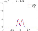
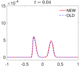
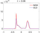
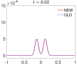
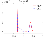
Figure 3.1: Example 2 (small perturbation): Time snapshots of the difference $h-h_{\rm eq}$ computed by the NEW and OLD schemes using a coarse mesh with $100$ cells (top row) and a finer mesh with $300$ cells (bottom row).

We now add a small Gaussian-shape perturbation to the stationary water depth and test the ability of the proposed schemes to accurately capture this small perturbation. In order to compare with the OLD scheme that a WB method is developed based on finite volume framework, we only “pollute” the cell average of water depth. That is, we add a small perturbation, which takes the form of $10^{-3}e^{-200x^{2}}$, to the initial cell average of water depth and compute the numerical solutions at three different times $t=0.02$, $0.04$, and $0.06$ using either $100$ or $300$ uniform cells by both the NEW and OLD schemes. The differences between the computed and background cell averages of water depth are plotted in Figure 3.1. As one can observe, the initial perturbation splits into two humps, which are then propagating into opposite directions, respectively. When the coarse mesh is used, the NEW scheme generates much more accurate results. In particular, at the final time $t=0.06$, the result at $x\approx 0.3$ computed by the NEW scheme is much shaper than its counterpart. When the mesh is refined, both of the two studied schemes converge to (almost) the same solution.

Example 3—Moving-Water Equilibria and Their Small Perturbations

In the third example, we verify the WB property of the NEW scheme in the sense that it is capable of exactly preserving moving-water equilibria (1.6). To this end, we consider a continuous bottom topography,

$$Z(x)=\left\{\begin{aligned} &0.2-0.05(x-10)^{2}&&\mbox{if}~{}8\leq x\leq 12,\\ &0&&\mbox{otherwise},\end{aligned}\right.$$ (3.1)

prescribed in a computational domain is $[0,25]$, and the following three sets of initial data that correspond to three different flow regimes (supercritical, subcritical, and transcritical without shock):

Case (a): $$q_{\rm eq}(x,0)\equiv 24, E_{\rm eq}(x,0)\equiv\frac{24^{2}}{2\times 2^{2}}+9.812\times 2;$$ (3.2)

Case (b): $$q_{\rm eq}(x,0)\equiv 4.42, E_{\rm eq}(x,0)\equiv\frac{4.42^{2}}{2\times 2^{2}}+9.812\times 2;$$

Case (c): $$q_{\rm eq}(x,0)\equiv 1.53, E_{\rm eq}(x,0)\equiv\frac{3}{2}(9.812\times 1.53)^{\frac{2}{3}}+9.812\times 0.2.$$

The relevant steady-state water depths $h_{\rm eq}(x,0)$ are computed in the same manner as introduced in [15, Remark 4.1] and given by

$$\mbox{Case (a):}~{}~{}h_{\rm eq}(x,0)=-\frac{a_{0}}{3}\Big{[}2\cos\big{(}\frac{\theta+4\pi}{3}\big{)}+1\Big{]},$$ (3.3)

$$\mbox{Case (b):}~{}~{}h_{\rm eq}(x,0)=-\frac{a_{0}}{3}\Big{[}2\cos\frac{\theta}{3}+1\Big{]},$$

$$\mbox{Case (c):}~{}~{}h_{\rm eq}(x,0)=\left\{\begin{aligned} &-\frac{a_{0}}{3}\Big{[}2\cos\big{(}\frac{\theta+4\pi}{3}\big{)}+1\Big{]}&&\quad\mbox{if}~{}x>10,\\ &-\frac{a_{0}}{3}\Big{[}2\cos\frac{\theta}{3}+1\Big{]}&&\quad\mbox{if}~{}x<10,\\ &-\frac{2a_{0}}{3}&&\quad\mbox{else},\end{aligned}\right.$$

where $a_{0}=\frac{gZ(x)-E_{\rm eq}(x,0)}{g}$, $a_{2}=\frac{(q_{\rm eq}(x,0))^{2}}{2g}$, and $\theta=\arccos(1+\frac{27a_{2}}{2a_{0}^{3}})$.

We first use the NEW scheme with 100 uniform cells to compute the numerical solutions until a final time $t=20$ for all the three cases mentioned above. The discrete $L^{1}$- and $L^{\infty}$-errors in the average values of $h$ and $q$ are computed and reported in Tables 3.4. It is clear that the NEW scheme can exactly preserve all three moving-water equilibria within machine accuracy.

Table 3.4: Example 3: $L^{1}$- and $L^{\infty}$-errors in average values of $h$ and $q$ over continuous bathymetry (3.1) .

	$L^{1}$-error in $h$	$L^{\infty}$-error in $h$	$L^{1}$-error in $q$	$L^{\infty}$-error in $q$
Case (a)	2.34e-13	2.51e-14	1.77e-12	2.38e-13
Case (b)	3.40e-14	6.22e-15	3.79e-13	4.62e-14
Case (c)	2.49e-14	3.94e-15	7.92e-14	1.20e-14

We then add a small perturbation, which takes the form of $10^{-3}e^{-80(x-6)^{2}}$, to the steady-state cell average of water depth $h_{\rm eq}(x,0)$ in (3.3). We compute the numerical solutions using the NEW and OLD schemes until $t=1$ in the supercritical case and until $t=1.5$ in the subcritical and transcritical cases. The difference between the obtained and the background moving steady-state cell averages of water depth computed with $100$ and $1000$ uniform cells are plotted in Figure 3.2. As one can observe, the propagating perturbations are well captured by both studied schemes over both coarse and fine meshes. Comparing the results obtained by the alternative OLD scheme, we can see that the NEW scheme produces much higher resolution solutions.

     

     

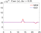
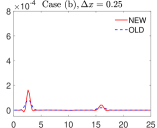
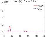
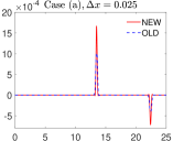
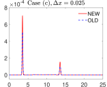
Figure 3.2: Example 3: The difference between the obtained and the steady-state cell averages of water depth computed by both the NEW and OLD schemes using uniform cells with mesh size $\Delta x=0.25$ (top row) and $\Delta x=0.025$ (bottom row) for Cases (a, left column), (b, middle column) and (c, right column).

Example 4—Convergence to Moving-Water Equilibria

In the fourth example, we study the convergence in time of the numerical solution computed by the proposed NEW scheme towards steady flow over the continuous bathemetry given by (3.1). Depending on the initial and boundary conditions, the obtained convergent flow may be supercritical, subcritical, or transcritical without or with a steady shock. The four sets of initial and boundary conditions in terms of water depth and velocity are summarized as follows:

Case (a): $$\left\{\begin{array}[]{l}h(x,0)=2-Z(x),\quad u(x,0)=0,\\ h(0,t)=2,\qquad\qquad~{}~{}u(0,t)=12;\end{array}\right.$$

Case (b): $$\left\{\begin{array}[]{l}h(x,0)=2-Z(x),\quad u(x,0)=0,\\ h(0,t)=2,\qquad\qquad~{}~{}u(0,t)=2.21,\quad h(25,t)=2;\end{array}\right.$$

Case (c): $$\left\{\begin{array}[]{l}h(x,0)=0.66-Z(x),\quad~{}u(x,0)=0,\\ h(0,t)=1.01439,\qquad\quad~{}u(0,t)=1.53/h(0,t),\quad h(25,t)=0.66;\end{array}\right.$$

Case (d): $$\left\{\begin{array}[]{l}h(x,0)=0.33-Z(x),\quad u(x,0)=0,\\ h(0,t)=0.41372,\qquad\quad u(0,t)=0.18/h(0,t),\quad h(25,t)=0.33.\end{array}\right.$$

Remark 3.2

In Case (c), the downstream boundary condition $(h(25,t)=0.66)$ is imposed only when the flow is subcritical.

The numerical solutions ($h+Z$, $q$, and $E$) at a final time $t=500$ on the computational domain $[0,25]$ computed by the NEW scheme with 200 uniform cells are depicted in Figure 3.3. As one can see, the numerical solutions of the first three cases have almost converged to the desired discrete steady states. However, for Case (d), like most of the existing schemes, the proposed scheme also fails to accurately resolve the equilibrium as the errors at the shock are $\mathcal{O}(1)$. It is easy to find that the numerical solutions obtained here are comparable with those reported in [8, 34, 14, 15].

     

     

     

     

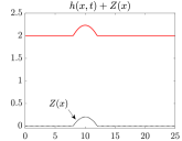
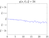
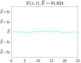
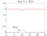
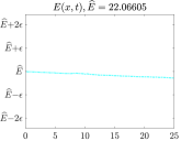
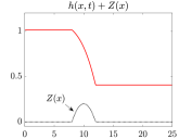
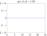
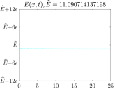
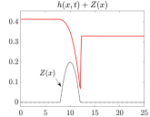
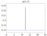
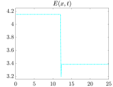
Figure 3.3: Example 4: Convergent solutions of $h+Z$ together with $Z$ (left column), $q$ (middle column) and $E$ (right column) for Cases (a, first row), (b, second row), (c, third row), and (d, fourth row). The small deviation parameter $\epsilon=10^{-12}$.

Example 5—Dam-break Problem

In the fifth example, we study a dam-break problem with a mixed Riemann solution, i.e., the solution consists of one rarefaction and one shock wave. The initial data are

$$(h(x,0),u(x,0),Z(x))=\left\{\begin{aligned} &(10,0,0),\quad&&x<0,\\ &(1,0,0),\quad&&x\geq 0.\\ \end{aligned}\right.$$

The exact solution of this problem is given by a left-propagating rarefaction and a right-propagating shock wave. We use both the NEW and OLD schemes to compute the numerical solutions at the final time $t=8$ in the computational domain $[-150,150]$ covered with $300$ uniform cells. Results are shown in Figure 3.4. As one can see, the obtained profiles of $h$ and $q$ provide expected results with a left-directed rarefaction and a right-directed shock wave. The numerical solutions computed by the two studied schemes are in a satisfactory agreement.

   

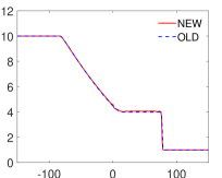
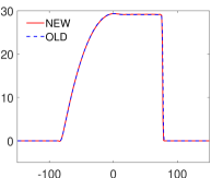
Figure 3.4: Example 5: Water depth $h$ (left) and discharge $q$ (right) computed by the NEW and OLD schemes.

Example 6—Riemann Problem

In the sixth example, we consider the following initial value problem in $[0,25]$ with the Riemann initial data to verify the positivity-preserving property of the NEW scheme:

$$h(x,0)=\left\{\begin{aligned} &2\quad&&\mbox{if}~{}x<5,\\ &0\quad&&\mbox{otherwise},\end{aligned}\right.\quad u(x,0)=\left\{\begin{aligned} &12\quad&&\mbox{if}~{}x<5,\\ &0\quad&&\mbox{otherwise},\end{aligned}\right.$$

subject to the Dirichlet boundary condition:

$$h(0,t)=2,\quad u(0,t)=12.$$

The bottom topography is given by (3.1). We compute the solutions using $100$ uniform cells at five different times: $t=0.2$, $0.5$, $1$, $2$, and $6$. The numerical solutions ($h+Z$, $q$, and $E$) of these time snapshots are plotted in Figure 3.5. As one can clearly observe that the water flow runs through the bottom hump and by $t=6$ it reaches the same discrete steady state as in Examples 3, case (a) as expected. The initial data contains dry area $(h=0)$ and the obtained results are stable and thus show that the proposed NEW scheme possesses the positivity-preserving property.

     

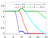
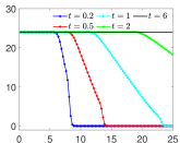
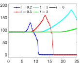
Figure 3.5: Example 6: Computed solutions of $h+Z$ together with $Z$ (left), $q$ (middle) and $E$ (right).

Example 7—Convergence to Moving-Water Equilibria for Frictional case

In the seventh example, which is a modification of Example 4, we now consider a nonzero Manning friction term and study the convergence in time of the numerical solution towards discrete steady states over a continuous hump given by (3.1). Three cases corresponding to the supercritical [Case (a)], subcritical [Case (b)], and transcritical flow with a steady shock [Case (d)] are taken into account. We take “lake-at-rest” initial conditions and the Dirichlet boundary conditions:

Case (a): $$\left\{\begin{array}[]{l}h(x,0)=2-Z(x),\quad u(x,0)=0,\\ h(0,t)=2,\qquad\qquad~{}~{}u(0,t)=12;\end{array}\right.$$

Case (b): $$\left\{\begin{array}[]{l}h(x,0)=2-Z(x),\quad u(x,0)=0,\\ h(0,t)=2.14618,\quad~{}~{}u(0,t)=4.42/h(0,t),\quad h(25,t)=2;\end{array}\right.$$

Case (d): $$\left\{\begin{array}[]{l}h(x,0)=0.33-Z(x),~{}~{}u(x,0)=0,\\ h(0,t)=0.44835,\quad\quad~{}~{}u(0,t)=0.18/h(0,t),\quad h(25,t)=0.32.\end{array}\right.$$

As in Example 4, we compute the numerical solutions using the proposed NEW scheme at time $t=500$ in the computational domain $[0,25]$ covered with $200$ uniform cells. We plot the obtained numerical solutions ($h+Z$, $q$, and $E$) in Figure 3.6. As one can see, the obtained numerical results are comparable with those reported in [34, 14]. We can therefore conclude that the proposed NEW scheme is also able to capture the steady states of different flow regimes in the presence of nonzero friction terms.

     

     

     

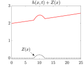
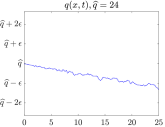
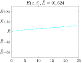
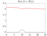
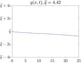
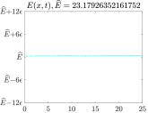
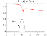
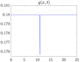
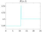
Figure 3.6: Example 7: Convergent solutions of $h+Z$ together with $Z$ (left column), $q$ (middle column) and $E$ (right column) for Cases (a, first row), (b, middle row), and (d, bottom row) with $n=0.05$ and the deviation number $\epsilon=10^{-12}$.

Example 8—Small Perturbation of Moving-Water Equilibria for Frictional case

In the final example, we test the ability of the proposed NEW scheme to capture small perturbations of the obtained discrete steady states of Cases (a) and (b) as shown in Example 7. Similar to Example 3, we add a small perturbation $10^{-3}e^{-80(x-6)^{2}}$ to the discrete steady-state cell average of water depth obtained from the following two sets of the discrete moving-water equilibria:

Case (a): $$q(x,0)\equiv 24,\quad E(x,0)\equiv 91.624;$$ (3.4)

Case (b): $$q(x,0)\equiv 4.42,\quad E(x,0)\equiv 23.17926352161752.$$

We note that the initial data in (3.4) is given in terms of the equilibrium variable $\bm{E}=(q,E)^{\top}$ rather than in $h$ and $u$. However, in order to start the computation at time $t=0$, one has to obtain the average values of $\hbox{\vbox{\hrule height=0.5pt\kern 1.72218pt\hbox{\kern-0.50003pt$h$\kern 0.0pt}}}_{j+\frac{1}{2}}$ and the point values of $h_{j}$. Unlike Example 3, here we use the Newton’s method to numerically solve the following nonlinear equations:

$$E_{j}=\frac{q_{j}^{2}}{2h_{j}^{2}}+g(h_{j}+Z_{j})+Q_{j},\quad E_{j+\frac{1}{2}}=\frac{q^{2}_{j+\frac{1}{2}}}{2h^{2}_{j+\frac{1}{2}}}+g(h_{j+\frac{1}{2}}+Z_{j+\frac{1}{2}})+Q_{j+\frac{1}{2}},\quad\forall j,$$

where $Q_{j+\frac{1}{2}}$ and $\{Q_{j}\}_{j>1}$ are computed from the recursive formula (2.9). After obtaining the point values of water depth, it is easy to compute the initial average values of $\hbox{\vbox{\hrule height=0.5pt\kern 1.72218pt\hbox{\kern-0.50003pt$h$\kern 0.0pt}}}_{j+\frac{1}{2}}$ using Simpson’s rule.

Equipped with the initial values in terms of water depth and velocity, we now compute the numerical solutions using the NEW scheme until $t=1$ and $t=1.5$ for Cases (a) and (b), respectively. The difference between the computed and the background discrete moving steady-state cell averages of water depth are plotted in Figure 3.7, where one can see that the proposed NEW scheme is able to accurately capture the small perturbation in a robust manner.

   

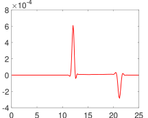
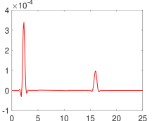
Figure 3.7: Example 8: The difference between the computed and the background discrete steady-state cell averages of water depth computed using 200 uniform cells for Cases (a, left) and (b, right).

4 Conclusion

In this paper, we have developed and tested new positivity-preserving well-balanced schemes for the one-dimensional (1-D) Saint-Venant system of shallow water equations with the Manning friction term. The main challenge in developing an accurate and robust well-balanced scheme for the 1-D shallow water equations is related to the fact that a special transformation between the conservative variables and the equilibrium variables is crucial to recover the moving water equilibrium; see, e.g., [8, 18, 19, 27, 14, 15, 40]. In the process of transformation, one needs to solve some (nonlinear) systems of equations and this can be cumbersome. In this work, we consider both the conservative and primitive forms of the studied hyperbolic system. More precisely, we use the former form to evolve the cell averages while use the latter one to evolve the point values. It is notice that using the introduced equilibrium variables, the primitive formulation will reduce to a very simple form with flux function only represented by the equilibrium variables. We then apply the finite difference method to compute the residuals, which will vanish when the solution is at the steady state. In order to update the average values in a WB manner, we use the equilibrium variables to rewrite the source term and apply Simpson’s rule to obtain the approximation of the source term. We also propose a way to guarantee the positivity property of water depth.

This study is only concerned with the one-dimensional shallow water equations but provides a new framework that does not require the transformation from equilibrium variables to conservative variables for designing fully WB methods. In future work, we plan to extend the proposed method to several space dimensions and other hyperbolic models including the thermal rotating shallow water equations, shallow water flows in channels, and the blood flow models.

Appendix A A third-order parabolic interpolant

In this appendix, we describe a third-order parabolic interpolant which is used in (2.8). Given the point value $\bm{U}_{j}$ and the cell average $\hbox{\vbox{\hrule height=0.5pt\kern 1.72218pt\hbox{\kern-0.50003pt$\bm{U}$\kern 0.0pt}}}_{j+\frac{1}{2}}$, we can construct a third-order parabolic interpolant:

$$\widetilde{\bm{U}}(x)=\bm{U}_{j}\ell_{0}(\xi)+\hbox{\vbox{\hrule height=0.5pt\kern 1.72218pt\hbox{\kern-0.50003pt$\bm{U}$\kern 0.0pt}}}_{j+\frac{1}{2}}\ell_{\frac{1}{2}}(\xi)+\bm{U}_{j+1}\ell_{1}(\xi),\quad\xi=\frac{x-x_{j}}{\Delta x}\in[0,1],$$ (A.1)

where

$$\ell_{0}(\xi)=(1-\xi)(1-3\xi),\quad\ell_{1}(\xi)=\xi(3\xi-2),\quad\ell_{\frac{1}{2}}(\xi)=6\xi(1-\xi).$$

Appendix B Desingularization

In this appendix, we describe the desingularization function, which we use whenever a division by zero or by a very small positive number needs to be avoided. Assume that we need to evaluate the quotient $a/b$ and that $b\sim 0$. We then use the simplest desingularization from [5] to compute the quotient as

$$\mathfrak{D}(a,b)=\left\{\begin{aligned} &\frac{a}{b}\quad&&\mbox{if}~{}b\geq\varepsilon,\\ &0\quad&&\mbox{otherwise}.\end{aligned}\right.$$ (B.1)

where $\varepsilon$ is small desingularization parameter which is set to $\varepsilon=10^{-9}$ in all of the reported numerical examples. Alternative desingularization functions can also be employed, the proposed schemes are not tight to these selections.

Appendix C Numerical diffusion switch function

In this appendix, we define the parameter $\Gamma_{j+\frac{1}{2}}$ as

$$\Gamma_{j+\frac{1}{2}}=\mathcal{H}(\eta_{j+\frac{1}{2}}),\quad\eta_{j+\frac{1}{2}}:=\frac{E_{j+1}-E_{j}}{\Delta x}\cdot\frac{\sum\limits_{j}|K_{j+\frac{1}{2}}|}{\max(E_{j+1},E_{j})},$$

where $\mathcal{H}(\eta)$ is a smooth cut-off function given by

$$\mathcal{H}(\eta):=\frac{(C\eta)^{m}}{1+(C\eta)^{m}}.$$

Note that $\Gamma_{j+\frac{1}{2}}$ is relatively small when the computed solution is locally (almost) at/near a steady state, while rapidly approaches $1$ when the solution is away from the steady state. Therefore, it will helps to switch off a part of the numerical diffusion when the computed solution is locally at/near steady states and thus ensure the WB property. In all of the numerical experiments reported in §3, we have used the constants $C=6$, $m=20$. For more descriptions of this numerical diffusion switch function, we refer to [16, 29, 8].

Appendix D Numerical tests over discontinuous bathymetries

Test 1

In this test, we consider the same initial setting as in Example 3 but over a discontinuous bathymetry:

$$Z(x)=\left\{\begin{aligned} &0.2&&\mbox{if}~{}8\leq x\leq 12,\\ &0&&\mbox{otherwise}.\end{aligned}\right.$$ (D.1)

In this case, the relevant steady-state water depth $h_{\rm eq}(x,0)$ for case (c) in (3.3) becomes

$$h_{\rm eq}(x,0)=\left\{\begin{aligned} &-\frac{a_{0}}{3}\Big{[}2\cos\big{(}\frac{\theta+4\pi}{3}\big{)}+1\Big{]}&&\quad\mbox{if}~{}x>12,\\ &-\frac{a_{0}}{3}\Big{[}2\cos\frac{\theta}{3}+1\Big{]}&&\quad\mbox{if}~{}x<8,\\ &\Big{(}\frac{q_{\rm eq}^{2}}{g}\Big{)}^{\frac{1}{3}}&&\quad\mbox{else}.\end{aligned}\right.$$

The same simulation as it was done in Example 3 is performed and we report the results in Table D.1 and Figure D.1. As one can see, the proposed scheme is able to exactly preserve the moving-water equilibrium and accurately capture the small perturbations even over a discontinuous bathymetry.

Table D.1: $L^{1}$- and $L^{\infty}$-errors in average values of $h$ and $q$ over discontinuous bathymetry (D.1).

	$L^{1}$-error in $h$	$L^{\infty}$-error in $h$	$L^{1}$-error in $q$	$L^{\infty}$-error in $q$
Case (a)	3.85e-13	4.02e-14	4.37e-12	4.26e-13
Case (b)	$<$1.0e-16	$<$1.0e-16	$<$1.0e-16	$<$1.0e-16
Case (c)	1.33e-14	2.50e-15	4.82e-14	9.10e-15

     

     

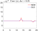
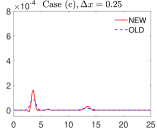
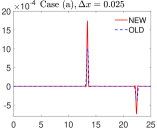
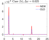
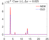
Figure D.1: Small perturbation: same as in Figure 3.2 but over discontinuous bathymetry (D.1).

Test 2

In this test, we repeat the simulation as it was done in Example 4, but with discontinuous bathymetry given by (D.1). The obtained results are reported in Figure D.2. As we can see, the expected convergent solutions are obtained and consistent with those produced by the well-balanced path-conservative central-upwind scheme in [8].

     

     

     

     

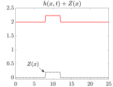
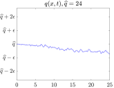
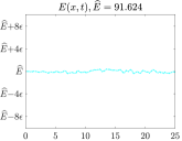
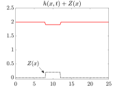
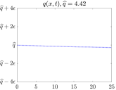
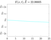
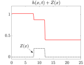
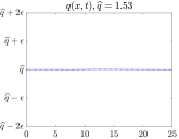
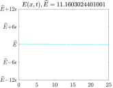
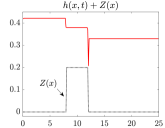
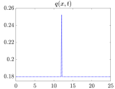
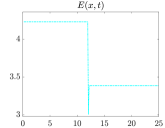
Figure D.2: Convergent solutions: Same as in Figure 3.3 but over discontinuous bathemetry (D.1).

Test 3

In this test, we study a problem associated with two rarefaction waves moving toward opposite directions. The initial data and bottom topography are

$$(h(x,0),u(x,0),Z(x))=\left\{\begin{aligned} &(8,-2,0),\quad&&x<0,\\ &(5,7.1704,1),\quad&&x\geq 0.\\ \end{aligned}\right.$$

The exact solution of this problem is given by a left-propagating 1-Rarefaction, a bottom step discontinuity, and a right-propagating 2-Rarefaction. We use both the NEW and OLD schemes to compute the numerical solutions at the final time $t=8$ in the computational domain $[-150,150]$ covered with $300$ uniform cells. Results are shown in Figure D.3. As one can see, the obtained water surface $h+Z$ profiles provide expected results with a left-directed rarefaction wave, a stationary shock, and a right-directed rarefaction wave. The numerical solutions computed by the two studied schemes are in a satisfactory agreement.

   

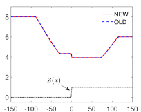
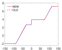
Figure D.3: Water surface $h+Z$ together with $Z$ (left) and velocity $u$ (right) computed by the NEW and OLD schemes.

References

- [1] R. Abgrall, A combination of Residual Distribution and the Active Flux formulations or a new class of schemes that can combine several writings of the same hyperbolic problem: application to the 1D Euler equation, Commun. Appl. Math. Comput., 5 (2023), pp. 370–402.
- [2] R. Abgrall and D. Torlo, Some preliminary results on a high order asymptotic preserving computationally explicit kinetic scheme, Commun. Math. Sci., 20 (2022), pp. 297–326.
- [3] E. Audusse, F. Bouchut, M.-O. Bristeau, R. Klein, and B. Perthame, A fast and stable well-balanced scheme with hydrostatic reconstruction for shallow water flows, SIAM J. Sci. Comput., 25 (2004), pp. 2050–2065.
- [4] W. Barsukow and J. P. Berberich, A well-balanced Active Flux method for the shallow watere quations with wetting and drying, Commun. Appl. Math. Comput., (2023). https://doi.org/10.1007/s42967-022-00241-x.
- [5] A. Bollermann, G. Chen, A. Kurganov, and S. Noelle, A well-balanced reconstruction of wet/dry fronts for the shallow water equations, J. Sci. Comput., 56 (2013), pp. 267–290.
- [6] A. Bollermann, S. Noelle, and M. Lukáčová-Medviďová, Finite volume evolution Galerkin methods for the shallow water equations with dry beds, Commun. Comput. Phys., 10 (2011), pp. 371–404.
- [7] S. Busto, M. Dumbser, S. Gavrilyuk, and K. Ivanova, On thermodynamically compatible finite volume methods and path-conservative ADER discontinuous Galerkin schemes for turbulent shallow water flows, J. Sci. Comput., 88 (2021). Paper No. 28, 45 pp.
- [8] Y. Cao, A. Kurganov, Y. Liu, and R. Xin, Flux globalization based well-balanced path-conservative central-upwind schemes for shallow water models, J. Sci. Comput, 92 (2022). Paper No. 69, 31 pp.
- [9] M. J. Castro, T. Morales de Luna, and C. Parés, Well-balanced schemes and path-conservative numerical methods, in Handbook of Numerical Methods for Hyperbolic Problems, vol. 18 of Handbook of Numerical Analysis, Elsevier/North-Holland, Amsterdam, 2017, pp. 131–175.
- [10] M. J. Castro, A. Pardo Milanés, and C. Parés, Well-balanced numerical schemes based on a generalized hydrostatic reconstruction technique, Math. Models Methods Appl. Sci., 17 (2007), pp. 2055–2113.
- [11] M. J. Castro and C. Parés, Well-balanced high-order finite volume methods for systems of balance laws, J. Sci. Comput., 82 (2020). Paper No. 48, 48 pp.
- [12] M. J. Castro Díaz, A. Kurganov, and T. Morales de Luna, Path-conservative central-upwind schemes for nonconservative hyperbolic systems, ESAIM Math. Model. Numer. Anal., 53 (2019), pp. 959–985.
- [13] M. J. Castro Díaz, J. A. López-García, and C. Parés, High order exactly well-balanced numerical methods for shallow water systems, J. Comput. Phys., 246 (2013), pp. 242–264.
- [14] Y. Cheng, A. Chertock, M. Herty, A. Kurganov, and T. Wu, A new approach for designing moving-water equilibria preserving schemes for the shallow water equations, J. Sci. Comput., 80 (2019), pp. 538–554.
- [15] Y. Cheng and A. Kurganov, Moving-water equilibria preserving central-upwind schemes for the shallow water equations, Commun. Math. Sci., 14 (2016), pp. 1643–1663.
- [16] A. Chertock, S. Cui, A. Kurganov, Ş. N. Özcan, and E. Tadmor, Well-balanced schemes for the Euler equations with gravitation: Conservative formulation using global fluxes, J. Comput. Phys., 358 (2018), pp. 36–52.
- [17] A. Chertock, S. Cui, A. Kurganov, and T. Wu, Well-balanced positivity preserving central-upwind scheme for the shallow water system with friction terms, Int. J. Numer. Methods Fluids, 78 (2015), pp. 355–383.
- [18] A. Chertock, A. Kurganov, X. Liu, Y. Liu, and T. Wu, Well-balancing via flux globalization: Applications to shallow water equations with wet/dry fronts, J. Sci. Comput., 90 (2022). Paper No. 9, 21 pp.
- [19] M. Ciallella, D. Torlo, and M. Ricchiuto, Arbitrary high order WENO finite volume scheme with flux globalization for moving equilibria preservation, (2022). arXiv preprint arXiv: 2205.13315.
- [20] S. Clain, S. Diot, and R. Loubère, A high-order finite volume method for systems of conservation laws—multi-dimensional optimal order detection (MOOD), J. Comput. Phys., 230 (2011), pp. 4028–4050.
- [21] G. Dal Maso, P. G. Lefloch, and F. Murat, Definition and weak stability of nonconservative products, J. Math. Pures Appl., 74 (1995), pp. 483–548.
- [22] U. S. Fjordholm, S. Mishra, and E. Tadmor, Well-balanced and energy stable schemes for the shallow water equations with discontinuous topography, J. Comput. Phys., 230 (2011), pp. 5587–5609.
- [23] J. Gallardo, C. Parés, and M. Castro, On a well-balanced high-order finite volume scheme for shallow water equations with topography and dry areas, J. Comput. Phys., 227 (2007), pp. 574–601.
- [24] S. Gottlieb, D. Ketcheson, and C.-W. Shu, Strong stability preserving Runge-Kutta and multistep time discretizations, World Scientific Publishing Co. Pte. Ltd., Hackensack, NJ, 2011.
- [25] S. Gottlieb, C.-W. Shu, and E. Tadmor, Strong stability-preserving high-order time discretization methods, SIAM Rev., 43 (2001), pp. 89–112.
- [26] S. Jin and X. Wen, Two interface-type numerical methods for computing hyperbolic systems with geometrical source terms having concentrations, SIAM J. Sci. Comput., 26 (2005), pp. 2079–2101. electronic.
- [27] C. Klingenberg, A. Kurganov, Y. Liu, and M. Zenk, Moving-water equilibria preserving HLL-type schemes forthe shallow water equations, Commun. Math. Res., 36 (2020), pp. 247–271.
- [28] A. Kurganov, Y. Liu, and R. Xin, Well-balanced path-conservative central-upwind schemes based on flux globalization, J. Comput. Phys., 474 (2023), p. 111773. 32 pp.
- [29] A. Kurganov, Y. Liu, and V. Zeitlin, A well-balanced central-upwind scheme for the thermal rotating shallow water equations, J. Comput. Phys., 411 (2020), p. 109414.
- [30] A. Kurganov and G. Petrova, A second-order well-balanced positivity preserving central-upwind scheme for the Saint-Venant system, Commun. Math. Sci., 5 (2007), pp. 133–160.
- [31] P. G. LeFloch, Hyperbolic systems of conservation laws, in The theory of classical and nonclassical shock waves, Lectures in Mathematics ETH Zürich, Birkhäuser Verlag, Basel, 2002.
- [32] , Graph solutions of nonlinear hyperbolic systems, J. Hyperbolic Differ. Equ., 1 (2004), pp. 643–689.
- [33] R. J. LeVeque, Balancing source terms and flux gradients in high-resolution Godunov methods: the quasi-steady wave-propagation algorithm, J. Comput. Phys., 146 (1998), pp. 346–365.
- [34] X. Liu, X. Chen, S. Jin, A. Kurganov, and H. Yu, Moving-water equilibria preserving partial relaxation scheme for the Saint-Venant system, SIAM J. Sci. Comput., 42 (2020), pp. A2206–A2229.
- [35] Y. Liu, J. Lu, Q. Tao, and Y. Xia, An oscillation-free Discontinuous Galerkin method for shallow water equations, J. Sci. Comput., 92 (2022). Paper No. 109, 24 pp.
- [36] S. Noelle, Y. Xing, and C.-W. Shu, High-order well-balanced finite volume WENO schemes for shallow water equation with moving water, J. Comput. Phys., 226 (2007), pp. 29–58.
- [37] M. Ricchiuto, An explicit residual based approach for shallow water flows, J. Comput. Phys., 280 (2015), pp. 306–344.
- [38] M. Ricchiuto and A. Bollermann, Stabilized residual distribution for shallow water simulations, J. Comput. Phys., 228 (2009), pp. 1071–1115.
- [39] F. Vilar, A posterior correction of high-order discontinuous Galerkin scheme through subcell finite volume formulation and flux reconstruction, J. Comput. Phys., 387 (2019), pp. 245–279.
- [40] Y. Xing, Exactly well-balanced discontinuous Galerkin methods for the shallow water equations with moving water equilibrium, J. Comput. Phys., 257 (2014), pp. 536–553.
- [41] Y. Xing and C.-W. Shu, A survey of high order schemes for the shallow water equations, J. Math. Study, 47 (2014), pp. 221–249.