Optimal Investment and Consumption Strategies with General and Linear Transaction Costs under CRRA Utility

Abstract

Transaction costs play a critical role in asset allocation and consumption strategies in portfolio management. We apply the methods of dynamic programming and singular perturbation expansion to derive the closed-form leading solutions to this problem for small transaction costs with arbitrary transaction cost structure by maximizing the expected CRRA (constant relative risk aversion) utility function for this problem. We also discuss in detail the case which consists of both fixed and proportional transaction costs.

Keywords: Portfolio management, transaction costs, optimal investment strategy, optimal consumption strategy, CRRA utility, asymptotic expansion.

1 Introduction

How to invest and how to consume are very important topics in modern finance and are also practical issues for fund managers. When transaction costs are neglected, optimal investment and consumption strategies, such as those in [29, 30], require dynamic trading of both risky and riskless assets, namely a fund manager needs to adjust the asset allocation continuously in time. This is not feasible in the presence of transaction costs which play critical roles in the determination of optimal investment allocation and consumption strategies. It naturally comes to the following questions: when should one adjust the portfolio, and how many shares of the risky asset should one buy or sell at the time of adjustment? What will be the optimal consumption strategy? We first present closed-form expressions for optimal investment and consumption strategies for transaction costs with a general payment structure but the amount of transaction is small relative to the total wealth, then focus on the common case which combines both fixed and proportional costs. A fixed cost is independent of the trading volume, and a proportional cost is proportional to the trading volume. The bid-ask spread is a typical example of proportional transaction costs. Since the fixed cost is levied on each trade regardless of its size, it plays a key role for small investors. Each investor has his/her own risk attitude that affects the person’s financial decision. Investors’ risk attitude is modeled by a utility function. Here we consider the constant relative risk aversion (CRRA) utility function.

In the presence of transaction costs, the well-known Merton strategy which requires continuous adjustment of the portfolio position becomes unfeasible, otherwise the wealth will be quickly depleted by transaction costs. Therefore, there exists a no-trade region in which the fund manager does not trade. When the price of the risky asset becomes sufficiently low, the fund manager will buy certain shares of the risky asset. Similarly, when the price of the risky asset becomes sufficiently high, the fund manager will sell certain shares of the risky asset. The questions are: At what price should the manager buy the risky asset? How many shares should the fund manager buy? At what price should the manager sell the risky asset? How many shares should the fund manager sell? Mathematically, these four important questions lead to four free boundaries and a nonlinear partial differential equation that governs the value function of the investment strategy and consumption strategy in the no-trade region. We derive the close-form leading order solutions to these important questions by applying the singular perturbation expansion in terms of the transaction costs since the magnitude of cost relative to the total wealth is usually small.

A large body of important research work on the optimal investment strategy is available in the literature. In the absence of transaction costs, Merton studied dynamic investment strategy based on the expected utility maximization and the dynamic programming approach, and gave the explicit solution to this optimization problem under CRRA utility function [29, 30]. Cox and Huang [9] and Karatzas et al. [21] characterized the optimal investment strategy with the martingale method. Cvitanic and Karatzas [10], He and Pearson [16] considered optimization problems with short-sale constraints, Korn and Trautmann [23] studied optimization problems with constraints on the terminal wealth, which allows handling the mean-variance problems. Zhang and Ge [15, 41] followed the expected utility maximization approach to study the optimal strategies for asset allocation and consumption under Henson stochastic volatility model [17].

The works mentioned above are for the cases of no transaction costs. Many important works are available in the literature for utility maximization with transaction costs included. In general, the transaction costs can be proportional or/and fixed.

For the case of a proportional transaction cost only, Magill and Constantinides [28] studied theoretically the optimal trading strategies with the proportional transaction costs, see also [8]. For the case of proportional transaction costs and infinite investment horizon, we refer to [1, 11, 26, 32, 36, 2, 13, 37]. Yang [40] gave an explicit asymptotic solution for a finite investment horizon based on the exponential utility function. Quek and Atkinson [35] studied the proportional transaction costs based on a power utility function in a multi-period discrete time setting. Janeček and Shreve [19] studied optimal investment and consumption strategies in an infinite horizon based on the power utility maximization. Kallsen and Muhle-Karbe [20] studied the optimal investment and consumption problem for a general utility function with small proportional transaction costs, and obtained the explicit leading-order formulas in an asymptotic expansion. Chellathurai and Draviam [7] studied optimal investment strategy for the case in which the coefficient in the proportional transaction costs depends on the trading volume.

For the case of a fixed transaction cost only in trading risky assets, we refer to [3, 27, 33]. Since the transaction is small, the perturbation method has been adopted in the study of optimal investment strategies with transaction costs. In particular, Morton and Pliska [33] considered logarithmic utility with a fixed transaction cost only for a long-term investor, and Altarovici et al. [3] considered independent multi-asset under power utility and in an infinite time horizon. For the case that agents face only fixed transaction costs, Lo et al. in [27] proposed a dynamic equilibrium model of asset prices and trading volume with a fixed transaction cost only.

For the cases in which the trading involves both proportional and fixed costs, we refer to the works [4, 6, 25, 22, 34]. Based on the exponential utility function, Liu [25] formulated the governing dynamic equations and free boundary conditions for multi-assets, and showed that these equations reduce to the one-risky-asset problem when all assets are independent. Furthermore, Liu studied numerically the case of two correlated risky assets. The method of Hamilton-Jacobi-Bellman quasi-variational inequality (HJBQVI) has also been applied to study the value function and the optimal control. We refer to [4, 6, 22, 34] the works in this approach in an infinite horizon. Altarovici et al. [4] and Cadenillas [6] considered a general utility and CRRA utility of consumption, respectively. Korn [22] studies the general utility of consumption in HJBQVI approach and derived a nontrivial asymptotically optimal solution for the problem of exponential utility maximization as an application. Øksendal and Sulem [34] studied the CRRA utility of consumption and presented some numerical estimates for the value function and the optimal consumption–investment policy.

The well-known Black-Scholes formulas for option prices are based on hedging the risk in the option by continuously trading the underlying asset. Therefore transaction costs are also very important in option pricing. For option pricing with the exponential utility and proportional transaction costs, we refer to [12, 38] for European options. Hodges and Neuberger [18] studied theoretically and numerically the option pricing problem under an exponential utility function with both proportional and fixed transaction costs. Whalley and Wilmott [39] derived an analytical solution for this model based on perturbation expansion.

In conclusion, we consider a financial market which consists of a riskless asset and a risky asset. We obtain the closed-form analytic solution for the optimal investment allocation strategy and for the optimal consumption strategy under both fixed and proportional transaction costs and under the general cost structure in a finite investment horizon. Our solutions are the leading-order solutions in terms of the magnitude of the ratio of transaction costs to total wealth. This ratio should be small in practice. Financially, here is the explanation of why this system is so complicated: In the absence of transaction costs, the optimal investment requires continuously adjusting the amount of wealth invested in the risky asset for the purpose of reducing the risks and enhancing the performance of the fund. Such a strategy is not practical in the presence of transaction costs, otherwise the wealth will be quickly depleted by the transaction costs. Therefore, there must exist a no-trade region in which the fund manager does not trade. When the price of the risky asset becomes sufficiently low, the fund manager will buy certain shares of the risky asset. Similarly, when the price of the risky asset becomes sufficiently high, the fund manager will sell certain shares of the risky asset. The questions are: At what price should the manager buy the risky asset? How many shares should the fund manager buy? At what price should the manager sell the risky asset? How many shares should the fund manager sell? These four important questions lead to four free boundaries in the mathematical formulation, and the nonlinear partial differential equation governs the value of the portfolio in the no-trade region.

The rest of this paper is organized as follows. In Section 2, we describe the basic model. In Section 3, we review the optimal investment and consumption policies in the absence of transaction costs under CRRA utility. In Section 4, we solve the problem with general transaction costs under CRRA utility and give leading-order solutions to optimal investment allocation, consumption policies and the value function. Section 5 derives the optimal policies under CRRA utility in the presence of three special structures of transaction costs, i.e. the combination of both fixed and proportional costs (linear cost), only fixed costs and only proportional costs. For the sake of readability, all mathematical proofs are located in Appendices A-D.

When there is only a fixed cost, we show that the optimal investment policy is to jump back to the Merton line when the proportional wealth in risky asset goes beyond a certain region. When there is only a proportional cost, the optimal behavior for investors is to trade in the minimal amount necessary to maintain the proportion of total wealth in the risky asset within a constant interval. The no-trade region in the above cases depends on the Merton line and the ratio of fixed costs to the total wealth or the proportional costs’ rate, respectively.

In addition, we prove that the liquidity of trading will decrease, regardless of whether fixed or proportional costs increase. Furthermore, unchanged the total wealth and fixed costs, the trading volume in the risky asset will decrease with the appearance of proportional costs. On the contrary, keeping the total wealth and proportional costs, the trading volume in the risky asset will increase with the appearance of fixed costs. These conclusions perfectly meet the natural characteristics of different costs.

Notation: Throughout this paper we assume a probability space $(\Omega,\mathcal{F},\mathbb{P})$, where $\mathbb{P}$ is a probability measure on $\Omega$, $\mathcal{F}$ is a $\sigma$-algebra. We endow the probability space $(\Omega,\mathcal{F},\mathbb{P})$ with an increasing filtration $\{\mathcal{F}_{t}\}_{t\geq 0}$, which is a right-continuous filtration on $(\Omega,\mathcal{F})$ such that $\{\mathcal{F}_{0}\}$ contains all the $\mathbb{P}$-negligible subsets. $\mathbb{E}[X]$ is the mathematical expectation of the stochastic process $X=X(\omega,t)$ with respect to $\mathbb{P}$. Uncertainty in the model is generated by a $\mathcal{F}_{t}$-adapted standard one-dimensional Brownian motion $W$. All stochastic integrals are defined in the sense of Itô. $C^{2}$-function respects a function with second continuous derivatives. ${\bf 1}_{\{\cdot\}}$ means the characteristic function.

2 The financial market, transaction costs and investor’s objectives

The Financial Market. We consider a financial market which consists of a risk-free asset $B$ and a risky asset $S$ governed by

$${\rm d}B(t)=rB(t){\rm d}t\ \ \text{and}\ \ {\rm d}S(t)=S(t)(\mu{\rm d}t+\sigma{\rm d}W),$$ (2.1)

where $r$ is the constant risk-free return rate, $\mu$ (assuming $\mu>r$) is the constant mean return, and $\sigma$ is the volatility of the risky asset $S$. Following [5, 14, 15, 17, 24, 31, 40], we assume that the risk premium $A=\frac{\mu-r}{\sigma^{2}}$ is constant, which means the stock excess return is proportional to the stock variance.

Transaction Costs. In this market, trading (buying or selling) the risky asset incurs a small transaction cost with a general form $k(n,S(t))$, where $n$ is the number of units of risky asset traded at the price $S(t)$. Throughout this paper, we require that $k(x,y)$ is a $C^{2}$-function.

The self-financing condition leads to the following equations for the amount of wealth in bank $w^{B}(t)$ and the amount of wealth in the risky asset $w^{S}(t)$

$${\rm d}w^{B}(t)=rw^{B}(t){\rm d}t-c(t){\rm d}t-{\rm d}\mathfrak{L}(t)+{\rm d}\mathfrak{J}(t)-k(n,S(t))\cdot{\bf 1}_{\{{\rm d}\mathfrak{L}(t)+{\rm d}\mathfrak{J}(t)>0\}}$$

$${\rm d}w^{S}(t)=w^{S}(t)(\mu{\rm d}t+\sigma{\rm d}W)+{\rm d}\mathfrak{L}(t)-{\rm d}\mathfrak{J}(t),$$

where $\mathfrak{L}$, $\mathfrak{J}$ represents the cumulative dollar amount of purchase and sale of the risky asset from the initial time, respectively. These processes are nondecreasing, right-continuous and adapted, with $\mathfrak{L}(0)=\mathfrak{J}(0)=0$. And $c(t)$ is the consumption rate at time $t$.

The Investor’s Objectives. An investor with an initial wealth $w_{0}$ has a CRRA utility function given by

$$u(x)=\left\{\begin{aligned} &\frac{ax^{\gamma}}{\gamma},\ \ \gamma<1,\ \ \gamma\neq 0,\\ &a\log(x),\ \ \gamma=0,\end{aligned}\right.$$ (2.2)

where $a$ is a positive constant. The absolute risk aversion (ARA) of (2.2) is

$${\rm ARA}(x)=-\frac{u^{\prime\prime}(x)}{u^{\prime}(x)}=\frac{1-\gamma}{x}>0.$$ (2.3)

The RRA of the CRRA utility function

$${\rm RRA}(x)=-\frac{xu^{\prime\prime}(x)}{u^{\prime}(x)}=1-\gamma$$ (2.4)

is a constant. At time $t$, the investor allocates $\phi(t)$ portion of his/her wealth $w(t)$, i.e. $\phi(t)w(t)$, to the risky asset, and $(1-\phi(t))w(t)$ to the risk-free asset. He/she consumes $c(t){\rm d}t$ over an infinitesimal time interval $[t,t+{\rm d}t]$, where $c(t)$ is the consumption rate at time $t$. Due to the presence of transaction costs, the investor will not continuously adjust the portfolio position. Therefore there is a no-trade region. When the price of the risky asset $S(t)$ reaches a certain low level (known as buy boundary $\phi_{B}$), the investor will buy some additional units of the risky asset. After buying, the portfolio will be located at a new position known as the post-buy boundary $\widehat{\phi}_{B}$. Similarly, there are sell and post-sell boundaries associated with the action of sell, denoted by $\phi_{S}$ and $\widehat{\phi}_{S}$ respectively, when the price of the risky asset is high enough. A sketch for these boundaries is shown in Figure 1. We comment that, in general, $\phi_{B}$, $\widehat{\phi}_{B}$, $\phi_{S}$ and $\widehat{\phi}_{S}$ are functions of time $t$, the price of the risky asset $S(t)$, and the wealth $w(t)$.

The investors’ objective is to maximize the expected utilities at the investment horizon $T$, by choosing an optimal consumption strategy $c(t)$ and an optimal asset allocation strategy $\phi(t)$,

$$\sup_{(c(t),\phi(t))\in\Theta(c(t),\phi(t))}\mathbb{E}\left[\int_{0}^{T}\alpha e^{-\beta t}u_{1}(c(t)){\rm d}t+(1-\alpha)e^{-\beta T}u_{2}(w(T))\right].$$ (2.5)

Here $\alpha$ measures the relative importance of these two utilities. $\beta$ is the subjective discount rate. $u_{1}(\cdot)$ is the CRRA utility function associated with the intermediate consumption, and $u_{2}(\cdot)$ is the CRRA utility function associated with the terminal wealth. They are given by the following functional forms:

$$u_{1}(c(t))=\left\{\begin{aligned} &\frac{a_{c}c(t)^{\gamma}}{\gamma},\quad\gamma\neq 0,\\ &a_{c}\log(c(t)),\quad\gamma=0,\end{aligned}\right.\quad\text{and}\quad u_{2}(w(T))=\left\{\begin{aligned} &\frac{a_{w}w(T)^{\gamma}}{\gamma},\quad\gamma\neq 0,\\ &a_{w}\log(w(T)),\quad\gamma=0.\end{aligned}\right.$$ (2.6)

Note that the constant $a_{c}$ can be different from $a_{w}$. The set

$$\Theta(c(t),\phi(t))\triangleq\left\{\int_{0}^{t}|c_{t^{\prime}}|{\rm d}t^{\prime}<\infty,\ w(t)-k(|\triangle\phi(t)|,w(t))\geq 0,\ \forall\ t\in[0,T]\right\}$$

represents all admissible trading and consumption strategies. The wealth process, based on $\phi(t)$ and $c(t)$, is

$${\rm d}w(t)=\phi(t)w(t)S^{-1}(t){\rm d}S(t)+r(1-\phi(t))w(t){\rm d}t-c(t){\rm d}t.$$ (2.7)

This optimal control problem is mathematically difficult. It needs to solve a nonlinear partial differential equation in the no-trade region and four free boundaries ($\phi_{B}$, $\widehat{\phi}_{B}$, $\phi_{S}$ and $\widehat{\phi}_{S}$). The no-trade region lies between $\phi_{B}$ and $\phi_{S}$ as shown in Figure 1. The four free boundaries $\phi_{B}$, $\widehat{\phi}_{B}$, $\phi_{S}$ and $\widehat{\phi}_{S}$ address four important questions: When to buy some additional risky asset? How many units to buy? When to sell some units of the risky asset? How many units are to sell? The optimal asset allocation strategy $\phi^{*}$ for no-transaction-cost case lies between $\phi_{B}$ and $\phi_{S}$, the post-buying boundary lies between $\phi_{B}$ and $\phi^{*}$, and the post-sell boundary lies between $\phi^{*}$ and $\phi_{S}$ (We will prove this relationship in Section 4).

Here is an intuitive explanation of Figure 1, before making a trading decision the investor needs to balance between wealth reduction in the transaction costs and the benefit from risk reduction. When the benefit from risk reduction is smaller than the transaction costs, the investor will not trade. This means the position of the portfolio is inside the no-trade region. When the price of the risky asset is sufficiently low, the benefit from risky reduction becomes more important than the loss in the transaction costs, and the investor will trade. This means the position of the portfolio is in the trading region. The phase boundary between the no-trade region and the trading region is the trade boundary $\phi_{B}$. The trading brings the position of the portfolio to $\widehat{\phi}_{B}$ which is inside the no-trade region. The interpretations for $\phi_{S}$ and $\widehat{\phi}_{S}$ are similar.

Let $\widetilde{V}(t,w,\phi)$ be the value function in this optimal investment and consumption problem

$$\widetilde{V}(t,w,\phi)=\sup_{(c(t),\phi(t))\in\Theta(c(t),\phi(t))}\mathbb{E}\left[\left.\int_{t}^{T}e^{-\beta t^{\prime}}\alpha u_{1}(c(t^{\prime})){\rm d}t^{\prime}+(1-\alpha)e^{-\beta T}u_{2}(w(T))\right|\mathcal{F}_{t}\right].$$ (2.8)

The terminal condition at the investment horizon $t=T$ is $\widetilde{V}(T,w,\phi)=(1-\alpha)e^{-\beta T}u_{2}(w(T))$. Let $\tau=T-t$ be the time to the end of the investment horizon. We express $\widetilde{V}(t,w,\phi)$ as

$$\widetilde{V}(t,w,\phi)=V(\tau,w,\phi)=e^{-\beta(T-\tau)}\frac{a_{w}w^{\gamma}}{\gamma}f(\tau,w,\phi)^{1-\gamma},$$ (2.9)

and $f(\tau,w,\phi)$ is to be determined with the condition $f(0,w,\phi)=(1-\alpha)^{\frac{1}{1-\gamma}}$.

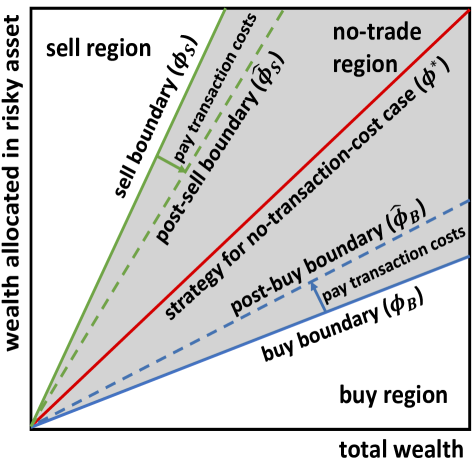
Figure 1: A sketch of optimal asset allocation strategies with transaction costs. There is a no-trade region (gray area) which contains the optimal allocation strategy for the no-transaction-cost case (red line). There are four free boundaries associated with the questions: When to buy/sell some risky asset, which determines the buy/sell boundary and how many units to buy/sell, which determines the post-buy/post-sell boundary?

There are a few constants which will appear frequently in our solutions. We define them here:

$$a_{1}=\left(\frac{\alpha a_{c}}{a_{w}}\right)^{\frac{1}{1-\gamma}},\quad a_{2}=\frac{\gamma\sigma^{2}}{2}a_{4}^{2}+\frac{\gamma r-\beta}{1-\gamma},\quad a_{3}=(1-\alpha)^{\frac{1}{1-\gamma}},\ \ a_{4}=\frac{A}{1-\gamma},$$ (2.10)

where $A=\frac{\mu-r}{\sigma^{2}}$. Throughout this paper, the time unit is measured in years and the wealth is measured in US dollars.

3 Optimal policies with no transaction costs

Since transaction costs are usually small, we will apply a singular expansion method near the solution for no-transaction-cost. Let us briefly describe the optimal investment and consumption strategies in the absence of transaction costs since it will serve as a base point for our singular perturbation expansion. The detail of the proof can be found in [29, 30, 31]. Based on the functional form

$$V^{*}(\tau,w)=e^{-\beta(T-\tau)}\frac{a_{w}w^{\gamma}}{\gamma}f^{*}(\tau)^{1-\gamma},$$ (3.1)

the Hamilton-Jacobi-Bellman (H-J-B) equation for $f^{*}$ is

$$\sup_{(c,\phi)\in\Theta(c,\phi)}\left\{\alpha e^{-\beta(T-\tau)}u_{1}(c)f^{*}-V^{*}\left[(1-\gamma)f^{*}_{\tau}-\left(\gamma r-\beta+\gamma A\sigma^{2}\phi-\frac{\gamma c}{w}+\frac{\gamma(\gamma-1)}{2}\sigma^{2}\phi^{2}\right)f^{*}\right]\right\}=0,$$ (3.2)

with $f^{*}(0)=a_{3}$. The optimal allocation strategy $\phi^{*}$ and the optimal consumption strategy $c^{*}$ are determined by the first-order derivative of (3.2),

$$\phi^{*}=\frac{A}{1-\gamma},\quad c^{*}(\tau,w)=a_{1}wf^{*}(\tau)^{-1}.$$ (3.3)

After substituting (3.3) into (3.2), it leads to

$$-f^{*}_{\tau}+a_{2}f^{*}+a_{1}=0,$$ (3.4)

which gives

$$f^{*}(\tau)=\left(\frac{a_{1}}{a_{2}}+a_{3}\right)e^{a_{2}\tau}-\frac{a_{1}}{a_{2}}.$$ (3.5)

The constants $a_{1},a_{2},a_{3}$, $a_{4}$ are defined in (2.10).

Expressions (3.3) and (3.1) serve as the base point for our singular perturbation expansion.

4 Optimal policies for general transaction cost structure

The optimal strategy in Section 3 requires trading continuously in time. This is not possible in the presence of transaction costs. In this section, we consider the transaction cost of a general form

$$k(\triangle\phi(t),w(t))$$ (4.1)

with the only restriction that $k(\cdot,\cdot)$ is a non-negative $C^{2}$-function. The transaction cost will make the adjustment of asset allocation infrequent. Otherwise, the wealth will be depleted in transaction costs. As shown by Figure 1, there is a no-trade region and associated trading boundaries. Within the no-trade region, no adjustment to the asset allocation will be made. When the price of the risky asset is sufficiently low, i.e. at the buy boundary $\phi_{B}$, one needs to buy additional risky assets which moves the portfolio’s position to the post-buy boundary $\widehat{\phi}_{B}$. Similarly, when the price of the risky asset is sufficiently high, i.e. at the sell boundary $\phi_{S}$, one will sell some risky asset which moves the portfolio’s position to the post-sell boundary $\widehat{\phi}_{S}$. We now determine the governing equation for the no-trade region and the boundary conditions for $\phi_{B}$, $\widehat{\phi}_{B}$, $\phi_{S}$ and $\widehat{\phi}_{S}$.

Governing equation in the no-trade region: Inside the no-trade region, only the consumption policy, $c$, is a control variable. From (2.1) and (2.7), we have

$${\rm d}(1-\phi(t))=\, {\rm d}\left(\frac{w^{B}(t)}{w(t)}\right)=\frac{1}{w(t)}{\rm d}w^{B}(t)+w^{B}(t){\rm d}\left(\frac{1}{w(t)}\right)$$

$$=\, \left[-(\mu-r)\phi(t)(1-\phi(t))+\sigma^{2}\phi(t)^{2}(1-\phi(t))-\frac{\phi(t)}{w(t)}c(t)\right]{\rm d}t-\sigma\phi(t)(1-\phi(t)){\rm d}W.$$

This gives

$${\rm d}\phi(t)=\left[\sigma^{2}\phi(t)(1-\phi(t))(A-\phi(t))+\frac{\phi(t)}{w(t)}c(t)\right]{\rm d}t+\sigma\phi(t)(1-\phi(t)){\rm d}W,$$ (4.2)

where $A=\frac{\mu-r}{\sigma^{2}}$. The H-J-B equation is

$$\sup_{c}\Big{\{} \alpha e^{-\beta(T-\tau)}u_{1}(c)-V_{\tau}+[(r+A\sigma^{2}\phi)w-c]V_{w}+\frac{1}{2}\sigma^{2}\phi^{2}w^{2}V_{ww}+\sigma^{2}\phi(1-\phi)(A-\phi)V_{\phi}$$

$$+\frac{\phi}{w}cV_{\phi}+\frac{1}{2}\sigma^{2}\phi^{2}(1-\phi)^{2}V_{\phi\phi}+\sigma^{2}\phi^{2}(1-\phi)wV_{w\phi}\Big{\}}=0,$$ (4.3)

with $V(0,w,\phi)=(1-\alpha)e^{-\beta T}u_{2}(w(T))$. From (2.6), (2.9) and (4), the optimal consumption strategy expressed in terms of $f$ is

$$c(\tau,w,\phi)=a_{1}wf^{-1}\left[1+\frac{1-\gamma}{\gamma}f^{-1}\left(wf_{w}-\phi f_{\phi}\right)\right]^{\frac{1}{\gamma-1}}.$$ (4.4)

After combining (2.6), (2.9), (4.4) and (4), we obtain the following governing equation inside the no-trade region with initial condition $f(0,w,\phi)=a_{3}$

$$-f_{\tau}+\left[h_{1}(\tau,\phi)-\sigma^{2}\phi^{2}\right](1-\phi)f_{\phi}+\left[r+h_{1}(\tau,\phi)\right]wf_{w}+\frac{1}{2}\sigma^{2}\phi^{2}(1-\phi)^{2}\left(f_{\phi\phi}-\gamma f^{-1}f^{2}_{\phi}\right)$$

$$+\frac{1}{2}\sigma^{2}\phi^{2}w^{2}\left(f_{ww}-\gamma f^{-1}f_{w}^{2}\right)+\sigma^{2}\phi^{2}(1-\phi)w\left(f_{w\phi}-\gamma f^{-1}f_{\phi}f_{w}\right)+h_{2}(\tau,\phi)f+a_{1}h_{3}(\tau,w,\phi,f)=0,$$ (4.5)

where $a_{1}$, $a_{3}$ are defined in (2.10), and

$$h_{1}(\tau,\phi)=A\sigma^{2}\phi+\gamma\sigma^{2}\phi^{2},$$

$$h_{2}(\tau,\phi)=\frac{\gamma r-\beta}{1-\gamma}+\frac{\gamma}{1-\gamma}\sigma^{2}A\phi-\frac{1}{2}\gamma\sigma^{2}\phi^{2},$$

$$h_{3}(\tau,w,\phi,f)=\left[1+\frac{1-\gamma}{\gamma}f^{-1}\left(wf_{w}-\phi f_{\phi}\right)\right]^{\frac{\gamma}{\gamma-1}}.$$

Governing equations for the four free boundaries: There are four free boundaries associated with this optimal control problem: the buy boundary $\phi_{B}$ at which one needs to increase the wealth allocated to the risky asset, the post-buy boundary $\widehat{\phi}_{B}$ associated with the additional amount of risky asset bought, the sell boundary $\phi_{S}$ at which one needs to reduce the wealth allocated to the risky asset, and the post-sell boundary $\widehat{\phi}_{S}$ associated with the amount of risky asset sold. We first discuss the conditions for determining the buy boundary $\phi_{B}$ and the post-buy boundary $\widehat{\phi}_{B}$. The value function at the buy and post-buy boundaries are the same, namely

$$V(\tau,w,\phi_{B})= V(\tau,\widehat{w}_{b},\widehat{\phi}_{B}),$$ (4.6)

where $w$ is the wealth before buying and $\widehat{w}_{b}=w+\triangle w_{b}$ is the wealth after buying. $\triangle w_{b}=-k(\widehat{\phi}_{B}-\phi_{B},w)$ is the transaction costs associated with the buying. The equation (4.6) can be expressed in terms of $f$:

$$f(\tau,w,\phi_{B})= \left(\frac{\widehat{w}_{b}}{w}\right)^{\frac{\gamma}{1-\gamma}}f(\tau,\widehat{w}_{b},\widehat{\phi}_{B}).$$ (4.7)

We optimize the expected utility by choosing when to buy ($\phi_{B}$), and how many units to buy ($\widehat{\phi}_{B}-\phi_{B}$). After applying the variation principle to (4.7) with respect to $\phi_{B}$ and $\widehat{\phi}_{B}$, respectively, we obtain

$$f_{\phi_{B}}(\tau,w,\phi_{B})=\, k_{\triangle\phi}(\widehat{\phi}_{B}-\phi_{B},w)\left\{\frac{\gamma}{1-\gamma}\widehat{w}_{b}^{-1}f(\tau,w,\phi_{B})+\left(\frac{\widehat{w}_{b}}{w}\right)^{\frac{\gamma}{1-\gamma}}f_{\widehat{w}}(\tau,\widehat{w}_{b},\widehat{\phi}_{B})\right\},$$ (4.8)

$$f_{\widehat{\phi}_{B}}(\tau,\widehat{w}_{b},\widehat{\phi}_{B})=\, k_{\triangle\phi}(\widehat{\phi}_{B}-\phi_{B},w)\left\{f_{\widehat{w}}(\tau,\widehat{w}_{b},\widehat{\phi}_{B})+\frac{\gamma}{1-\gamma}\left(\frac{\widehat{w}_{b}}{w}\right)^{-\frac{1}{1-\gamma}}w^{-1}f(\tau,w,\phi_{B})\right\}.$$ (4.9)

These three boundary conditions, (4.7)-(4.9), determine $\phi_{B}$ and $\widehat{\phi}_{B}$. Similarly, the following three equations determine $\phi_{S}$ and $\widehat{\phi}_{S}$:

$$f(\tau,w,\phi_{S})=\, \left(\frac{\widehat{w}_{s}}{w}\right)^{\frac{\gamma}{1-\gamma}}f(\tau,\widehat{w}_{s},\widehat{\phi}_{S}),$$ (4.10)

$$f_{\phi_{S}}(\tau,w,\phi_{S})=\, -k_{\triangle\phi}\left(\phi_{S}-\widehat{\phi}_{S},w\right)\left\{\frac{\gamma}{1-\gamma}\widehat{w}_{s}^{-1}f(\tau,w,\phi_{S})+\left(\frac{\widehat{w}_{s}}{w}\right)^{\frac{\gamma}{1-\gamma}}f_{\widehat{w}}(\tau,\widehat{w}_{s},\widehat{\phi}_{S})\right\},$$ (4.11)

$$f_{\widehat{\phi}_{S}}(\tau,\widehat{w}_{s},\widehat{\phi}_{S})=\, -k_{\triangle\phi}\left(\phi_{S}-\widehat{\phi}_{S},w\right)\left\{f_{\widehat{w}}(\tau,\widehat{w}_{s},\widehat{\phi}_{S})+\frac{\gamma}{1-\gamma}\left(\frac{\widehat{w}_{s}}{w}\right)^{-\frac{1}{1-\gamma}}w^{-1}f(\tau,w,\phi_{S})\right\},$$ (4.12)

where $w$ is the wealth before selling and $\widehat{w}_{s}=w+\triangle w_{s}$ is the wealth after selling. $\triangle w_{s}=-k(\phi_{S}-\widehat{\phi}_{S},w)$ is the transaction costs associated with the sale.

As we will prove later on, the post-trading boundaries $\widehat{\phi}_{B}$ and $\widehat{\phi}_{S}$ lie inside the no-trade region, that is $\phi_{B}\leq\widehat{\phi}_{B}\leq\phi^{*}\leq\widehat{\phi}_{S}\leq\phi_{S}$ (see Figure 1 and Section 3). Here $\phi^{*}$ is the optimal asset allocation strategy for the no-transaction-cost case. Therefore, the no-trade region is defined by

$$\text{No-trade region}\triangleq\{\phi\in\Theta(c,\phi):\ \phi_{B}\leq\phi\leq\phi_{S}\}.$$

In summary, to obtain optimal investment and consumption strategies, one needs to solve the nonlinear partial differential equation in the no-trade region given by (4) with six boundary conditions, namely three boundary conditions associated with the buy and post-buy positions given by (4.7)-(4.9), and three boundary conditions associated with the sell and post-sell positions given by (4.10)-(4.12).

The transaction costs relative to the total wealth usually are small. Therefore, we will apply the singular perturbation expansion method to solve the optimal asset allocation and consumption strategies. The base of the expansion is the no-transaction-cost case. Solutions to these equations, up to the leading order in terms of transaction costs, are given by the following theorem:

Theorem 4.1.

For a small transaction cost with an arbitrary structure $k(x,w)$, the leading order solutions to (4) and (4.7)-(4.12), in terms of transaction costs, are the following:

1. The optimal buy boundary $\phi_{B}$, post-buy boundary $\widehat{\phi}_{B}$, sell boundary $\phi_{S}$, and post-sell boundary $\widehat{\phi}_{S}$ are given by

   $$\phi_{S}=\phi^{*}+\frac{1}{2}\left(\tilde{x}+x\right),\ \widehat{\phi}_{S}=\phi^{*}+\frac{1}{2}\left(\tilde{x}-x\right),$$ (4.13)

   $$\phi_{B}=\phi^{*}-\frac{1}{2}\left(\tilde{x}+x\right),\ \widehat{\phi}_{B}=\phi^{*}-\frac{1}{2}\left(\tilde{x}-x\right).$$ (4.14)

   Here $x$ and $\tilde{x}$ are the unique nonnegative real roots of the following equations

   $$\left(\tilde{x}^{2}-x^{2}\right)\tilde{x}=A_{2}(x,w),\ x^{3}\tilde{x}=A_{1}(x,w),$$ (4.15)

   where

   $$A_{1}(x,w)=H\frac{k(x,w)-xk_{x}(x,w)}{w},\ A_{2}(x,w)=H\frac{k_{x}(x,w)}{w},\ \text{and}\ H=12\frac{\phi^{*^{2}}}{1-\gamma}\left(1-\frac{A}{1-\gamma}\right)^{2}.$$ (4.16)

2. The optimal value function is

   $$V(\tau,w)=V^{*}(\tau,w)\left[1+(1-\gamma)f^{*}(\tau)^{-1}\widehat{f}(\tau,w)\right].$$ (4.17)

3. The optimal consumption rate is

   $$c(\tau,w)= c^{*}(\tau,w)-a_{1}wf^{*}(\tau)^{-2}\left[\widehat{f}(\tau,w)+\frac{1}{\gamma}w\widehat{f}_{w}(\tau,w)\right].$$ (4.18)

In (4.17) and (4.18), $\widehat{f}(\tau,w)$ is

$$\widehat{f}(\tau,w)=-\gamma\sigma^{2}\psi(\tau)\left(3\tilde{x}^{2}+x^{2}\right),$$ (4.19)

where

$$\psi(\tau)=\,\frac{1}{24}\left[e^{a_{2}\tau}\frac{a_{2}(a_{1}+a_{2}a_{3})\tau-a_{1}}{a_{2}^{2}}+\frac{a_{1}}{a_{2}^{2}}\right].$$ (4.20)

The constants $a_{1},a_{2},a_{3}$ and $a_{4}$ are defined in (2.10).

In (4.13)-(4.20), $\phi^{*}$, $c^{*}$, $f^{*}$, and $V^{*}$ are the solution for the no-transaction-cost case. They are given by (3.3), (3.5) and (3.1), respectively.

Proof.

See Appendix A. ∎

From (4.16), it is easy to see that if both $A_{1}(x,w)$ and $A_{2}(x,w)$ are zero, $k(x,w)$ must be identically zero which corresponds to the case of no-transaction-cost. Therefore, we do not need to consider this case from now on.

Remark 1.

Here, we show how to solve (4.15) and prove the existence of the unique nonnegative solution for this equation.

1. When $A_{1}(x,w)\neq 0$, $A_{2}=0$, (4.15) becomes $\left(\tilde{x}^{2}-x^{2}\right)\tilde{x}=0$, $x^{3}\tilde{x}=A_{1}$. It leads to

   $$x=\tilde{x}=A_{1}^{\frac{1}{4}}(x,w).$$ (4.21)

   This recovers the solution in Theorem 5.1.

2. When $A_{1}(x,w)=0$, $A_{2}(x,w)\neq 0$, (4.15) becomes $\left(\tilde{x}^{2}-x^{2}\right)\tilde{x}=A_{2}(x,w)$, $x^{3}\tilde{x}=0$. It leads to

   $$x=0,\ \tilde{x}=A_{2}^{\frac{1}{3}}(x,w).$$ (4.22)

   This recovers the solution in Corollary 5.2.

3. When both $A_{1}(x,w)$ and $A_{2}(x,w)$ are nonzero, (4.15) can be written as

   $$A_{2}(x,w)x^{9}+A_{1}(x,w)x^{8}=A_{1}^{3}(x,w),$$ (4.23)

   $$\tilde{x}=\frac{A_{1}(x,w)}{x^{3}}.$$ (4.24)

   One can solve $x$ from (4.23) first, then obtain $\tilde{x}$ from (4.24). This recovers the solution in Corollary 5.1.

In cases (1) or (2), it is obvious the obtained solution is nonnegative and unique. In the general case (3) in which both $A_{1}(x,w)$ and $A_{2}(x,w)$ are nonzero, by applying the Descartes’ rule of signs, (4.23) has a unique positive real root for $x$. From (4.24), $\tilde{x}$ is also positive and unique. Therefore, we show that (4.15) has a unique nonnegative real root for all $A_{1}(x,w)$, $A_{2}(x,w)$.

Remark 2.

According to (4.13), (4.14), it is obvious that for small transaction costs, i.e. small $A_{1}(x,w)$, $A_{2}(x,w)$, the post-sell boundary is smaller than the sell boundary, and the post-buy boundary is larger than the buy boundary, namely $\phi_{B}\leq\widehat{\phi}_{B}\leq\phi^{*}\leq\widehat{\phi}_{S}\leq\phi_{S}$. In other words, the post-trading boundaries are inside the no-trade region.

Remark 3.

(4.15) shows that $\tilde{x}\neq 0$ unless both $A_{1}(x,w)$ and $A_{2}(x,w)$ equal to zero at the same time which is the case of no-transaction-cost. Therefore, the no-trade region always exists whenever there is a transaction cost.

The transaction cost plays an important role in investment and consumption strategies. In particular, it is important to know how transaction costs $A_{1}(x,w)$ and $A_{2}(x,w)$ in (4.16) affect the buy boundary $\phi_{B}$, post-buy boundary $\widehat{\phi}_{B}$, sell boundary $\phi_{S}$, and post-sell boundary $\widehat{\phi}_{S}\,$? The answer to this question is given by the following theorem.

Theorem 4.2.

Let $\phi_{B}$, $\widehat{\phi}_{B}$, $\phi_{S}$, and $\widehat{\phi}_{S}$ be, respectively, the optimal buy, post-buy, sell, and post-sell boundaries specified in Theorem 4.1 for given $\tau$, $w$, $A_{1}(x,w)$ and $A_{2}(x,w)$. Then

1. For fixed $A_{2}(x,w)$, $\phi_{S}$ increases, $\phi_{B}$ decreases with $A_{1}(x,w)$. Therefore, the no-trade region will be widened with $A_{1}(x,w)$. Furthermore, $\widehat{\phi}_{S}$ decreases, $\widehat{\phi}_{B}$ increases with $A_{1}(x,w)$. Consequently, both trading size for buy $|\widehat{\phi}_{B}-\phi_{B}|$ and that for sell $|\widehat{\phi}_{S}-\phi_{S}|$ increase with $A_{1}(x,w)$.

2. For fixed $A_{1}(x,w)$, $\phi_{S}$ increases, $\phi_{B}$ decreases with $A_{2}(x,w)$. Therefore, the no-trade region will be widened with $A_{2}(x,w)$. Although $\widehat{\phi}_{S}$ increases, $\widehat{\phi}_{B}$ decreases with $A_{2}(x,w)$, but both $|\widehat{\phi}_{B}-\phi_{B}|$ and $|\widehat{\phi}_{S}-\phi_{S}|$ decrease with $A_{2}(x,w)$. Thus, the trading size for buy and that for sell decrease with $A_{2}(x,w)$.

Proof.

See Appendix D. ∎

5 Optimal policies for fixed and proportional transaction costs

In this section, we study optimal investment and consumption strategies for a common transaction cost form which consists of both fixed and proportional transaction costs

$$k(|\triangle\phi|,w)=k_{1}+k_{2}|\triangle\phi|w,$$ (5.1)

where $k_{1}$ is the fixed cost, and $k_{2}$ is the rate of proportional cost. We will also analyze the special cases in which the transaction cost contains only the fixed cost or only the proportional cost.

For the fixed and proportional transaction costs given by (5.1), $f(\tau,w,\phi)$ inside the no-trade region is still governed by (4) and the optimal consumption policy $c$ is still given by (4.4). Two boundary conditions given by (4.7) and (4.10) remain the same. The remaining four boundary conditions can be easily deduced from (4.8) ,(4.9) , (4.11) and (4.12). The results are

$$f_{\phi_{B}}(\tau,w,\phi_{B})=k_{2}w\left\{\frac{\gamma}{1-\gamma}\widehat{w}_{b}^{-1}f(\tau,w,\phi_{B})+\left(\frac{\widehat{w}_{b}}{w}\right)^{\frac{\gamma}{1-\gamma}}f_{\widehat{w}}(\tau,\widehat{w},\widehat{\phi}_{B})\right\},$$ (5.2)

$$f_{\widehat{\phi}_{B}}(\tau,\widehat{w}_{b},\widehat{\phi}_{B})=k_{2}w\left\{f_{\widehat{w}}(\tau,\widehat{w}_{b},\widehat{\phi}_{B})+\frac{\gamma}{1-\gamma}\left(\frac{\widehat{w}_{b}}{w}\right)^{-\frac{1}{1-\gamma}}w^{-1}f(\tau,w,\phi_{B})\right\},$$ (5.3)

$$f_{\phi_{S}}(\tau,w,\phi_{S})=-k_{2}w\left\{\frac{\gamma}{1-\gamma}\widehat{w}_{s}^{-1}f(\tau,w,\phi_{S})+\left(\frac{\widehat{w}_{s}}{w}\right)^{\frac{\gamma}{1-\gamma}}f_{\widehat{w}}(\tau,\widehat{w}_{s},\widehat{\phi}_{S})\right\},$$ (5.4)

$$f_{\widehat{\phi}_{S}}(\tau,\widehat{w}_{s},\widehat{\phi}_{S})=-k_{2}w\left\{f_{\widehat{w}}(\tau,\widehat{w}_{s},\widehat{\phi}_{S})+\frac{\gamma}{1-\gamma}\left(\frac{\widehat{w}_{s}}{w}\right)^{-\frac{1}{1-\gamma}}w^{-1}f(\tau,w,\phi_{S})\right\},$$ (5.5)

where $\widehat{w}_{b}=w+\triangle w_{b}$, $\triangle w_{b}=-[k_{1}+k_{2}(\widehat{\phi}_{B}-\phi_{B})w]$ for the case of buying; $\widehat{w}_{s}=w+\triangle w_{s}$, $\triangle w_{s}=-[k_{1}+k_{2}(\phi_{S}-\widehat{\phi}_{S})w]$ for the case of sell. Therefore, for the fixed and proportional transaction costs, the system is governed by (4.4), (4), (4.7), (4.10), and (5.2)-(5.5).

The explicit solutions for $c$, $f$, $\phi_{B}$, $\widehat{\phi}_{B}$, $\phi_{S}$, and $\widehat{\phi}_{S}$, up to the leading order in terms of transaction costs, can be deduced from Theorem 4.1 and stated in the following.

Theorem 5.1 (for both fixed and proportional costs).

We will use a superscript $``fp"$ on a quantity to represent that the quantity is for the case of both fixed and proportional transaction costs given by (5.1), which is also known as the linear transaction costs.

For the linear transaction costs given by (5.1), the optimal trading boundaries are

$$\phi^{fp}_{S}= \phi^{*}+\frac{1}{2}\left(\tilde{x}^{fp}+x^{fp}\right),\quad\widehat{\phi}^{fp}_{S}=\phi^{*}+\frac{1}{2}\left(\tilde{x}^{fp}-x^{fp}\right),$$ (5.6)

$$\phi^{fp}_{B}= \phi^{*}-\frac{1}{2}\left(\tilde{x}^{fp}+x^{fp}\right),\quad\widehat{\phi}^{fp}_{B}=\phi^{*}-\frac{1}{2}\left(\tilde{x}^{fp}-x^{fp}\right),$$ (5.7)

where $x^{fp}$ and $\tilde{x}^{fp}$ are the unique nonnegative real roots of (4.15) with

$$A_{1}(x,w)=H\frac{k_{1}}{w},\ A_{2}(x,w)=Hk_{2},$$ (5.8)

and $H$ is defined in (4.16).

The optimal value function and consumption rate are

$$V^{fp}(\tau,w)=\, V^{*}(\tau,w)\left[1+(1-\gamma)f^{*}(\tau)^{-1}\widehat{f}^{fp}(\tau,w)\right],$$ (5.9)

$$c^{fp}(\tau,w)=\, c^{*}(\tau,w)+a_{1}{\gamma\sigma^{2}}\left[3\left(\tilde{x}^{fp}\right)^{2}+\left(x^{fp}\right)^{2}-\frac{2}{\gamma}\frac{H\frac{k_{1}}{w}}{x^{fp}\tilde{x}^{fp}}\right]f^{*}(\tau)^{-2}\psi(\tau)w.$$ (5.10)

In (5.9),

$$\widehat{f}^{fp}(\tau,w)=-{\gamma\sigma^{2}}\psi(\tau)\left(3\left(\tilde{x}^{fp}\right)^{2}+\left(x^{fp}\right)^{2}\right),$$ (5.11)

where $\psi(\tau)$ is given by (4.20), and $a_{1},a_{2},a_{3}$, $a_{4}$ are defined in (2.10).

In (5.6)-(5.11), $V^{*}$, $f^{*}$, $\phi^{*}$, $c^{*}$ are solutions for the no-transaction-cost case, which are given by (3.1), (3.5) and (3.3). Note that, in this case, $A_{1}(x,w)$ is independent of $x$, and $A_{2}(x,w)$ is independent of both $x$ and $w$.

Proof.

See Appendix B. ∎

We comment that the four critical boundaries $\phi_{B}$, $\widehat{\phi}_{B}$, $\phi_{S}$, $\widehat{\phi}_{S}$ have no explicit time dependence. They only implicitly depend on time through $w$ in $A_{1}(x,w)$ given by (5.8), since $w$ depends on time.

The following two corollaries give the special cases of Theorem 5.1, namely the case of fixed cost only and the case of proportional cost only.

Obtained the leading order solution for the case of fixed transaction cost only. The following corollary shows that our solutions indeed recover the work of [3, 33].

Corollary 5.1 (for the case of fixed cost only).

We will use a superscript “f” on a quantity to represent that the quantity is for the case of fixed transaction cost only. In this case, $k_{2}=0$ in (5.1), the optimal trading boundaries are

$$\phi^{f}_{S}=\phi^{*}+\left(H\frac{k_{1}}{w}\right)^{\frac{1}{4}},\ \phi^{f}_{B}=\phi^{*}-\left(H\frac{k_{1}}{w}\right)^{\frac{1}{4}},\ \widehat{\phi}^{f}_{S}=\widehat{\phi}^{f}_{B}=\phi^{*},$$ (5.12)

where $H$ and $\phi^{*}$ are given by (4.16) and (3.3). Moreover, the optimal value function and consumption policies are

$$V^{f}(\tau,w)=\, V^{*}(\tau,w)\left[1+(1-\gamma)f^{*}(\tau)^{-1}\widehat{f}^{f}(\tau,w)\right],$$ (5.13)

$$c^{f}(\tau,w)=\, c^{*}(\tau,w)+2a_{1}(2\gamma-1)\sigma^{2}\left(H\frac{k_{1}}{w}\right)^{\frac{1}{2}}f^{*}(\tau)^{-2}\psi(\tau)w.$$ (5.14)

In (5.13),

$$\widehat{f}^{f}(\tau,w)=-4{\gamma\sigma^{2}}\psi(\tau)\left(H\frac{k_{1}}{w}\right)^{\frac{1}{2}},$$ (5.15)

where $\psi(\tau)$ is given by (4.20), and $a_{1},a_{2},a_{3},a_{4}$ are defined by (2.10). $c^{*}$, $V^{*}$ and $f^{*}$ are given by (3.3), (3.1) and (3.5), respectively.

Equation (5.12) shows that

$$\phi^{f}_{B}-\phi^{*}=-\left({H\frac{k_{1}}{w}}\right)^{1/4},\quad\phi^{f}_{S}-\phi^{*}=\left(H\frac{k_{1}}{w}\right)^{1/4}.$$ (5.16)

Equation (5.16) shows that, as fixed cost $k_{1}$ increases, the buy boundary decreases and the sell boundary increases. Therefore, the optimal no-trade region widens, and the investor will trade less frequently. Equation (5.16) also shows that, as wealth $w$ increases, the buy boundary increases and the sell boundary decreases. Therefore, the optimal no-trade region narrows, and the investor will trade more frequently. These behavior are consistent with our intuition.

Obtained the leading order solution for the case of proportional transaction cost only. The following corollary shows that our solutions indeed recover the work of [19].

Corollary 5.2 (for the case of proportional cost only).

We will use a superscript “p” on a quantity to represent that the quantity is for the case of the proportional transaction cost only. For this case, $k_{1}=0$ in (5.1), the optimal trading boundaries are

$$\phi^{p}_{S}=\widehat{\phi}^{p}_{S}=\phi^{*}+\frac{1}{2}(Hk_{2})^{\frac{1}{3}},\quad\phi^{p}_{B}=\widehat{\phi}^{p}_{B}=\phi^{*}-\frac{1}{2}(Hk_{2})^{\frac{1}{3}},$$ (5.17)

where $H$ and $\phi^{*}$ are given by (4.16) and (3.3).

Moreover, the corresponding optimal value function and consumption policy are

$$V^{p}(\tau,w)=\, V^{*}(\tau,w)\left[1+(1-\gamma)f^{*}(\tau)^{-1}\widehat{f}^{p}(\tau,w)\right],$$ (5.18)

$$c^{p}(\tau,w)=\, c^{*}(\tau,w)+3a_{1}\gamma\sigma^{2}\left(Hk_{2}\right)^{\frac{2}{3}}f^{*}(\tau)^{-2}\psi(\tau)w,$$ (5.19)

In (5.18),

$$\widehat{f}^{p}(\tau)=-3{\gamma\sigma^{2}}\psi(\tau)(Hk_{2})^{\frac{2}{3}},$$ (5.20)

where $\psi(\tau)$ is given by (4.20), and $a_{1},a_{2},a_{3},a_{4}$ are defined by (2.10). $c^{*}$, $V^{*}$ and $f^{*}$ are given by (3.3), (3.1) and (3.5), respectively.

One can also understand the results $\widehat{\phi}_{B}=\phi_{B}$ and $\widehat{\phi}_{S}=\phi_{S}$ for the case of only proportional transaction cost in an intuitive way. When the portfolio sits on the trading boundaries $\phi_{B}$ or $\phi_{S}$. Then the next moment, there are two possibilities: (1) the portfolio is still on the trading boundary or moves to the inside of the no-trade region. In this case, no trading is needed. (2) the portfolio moves to the outside of the no-trade region. In this case, one only needs to trade as small an amount of the risky asset as possible to bring the portfolio to the trading boundary. This minimizes the transaction cost. If one moved the portfolio to the inside of the no-transaction region, a certain portion of the proportional transaction cost would be wasted as after trading the portfolio had the chance of moving to the inside of the no-trade region in the following moment.

We comment that, as the proportional costs’ rate $k_{2}$ increases, the optimal buying boundary $\phi_{B}$ will decrease and the optimal sell boundary $\phi_{S}$ will increase. Therefore, an increment in $k_{2}$ will widen the no-trade range and make the investor trade less frequently.

6 Conclusion

In this paper, we derive the analytical leading order solution in terms of the transaction costs for the optimal asset allocation and consumption strategies based on the maximization of the expected CRRA utility function. Transaction costs play a very important role in portfolio management and risk management. The well-known Merton strategy for portfolio management requires continuous adjustment of portfolio position and is not applicable in the presence of transaction costs. Our solution is for a general transaction cost with an arbitrary payment structure. In particular, we provide detailed discussions of the commonly encountered transaction cost forms which consist of both fixed and proportional costs. It is well known that for the case of fixed transaction cost, only the no-trade region is proportional to the one-fourth power of the fixed cost, and for the case of proportional transaction cost only the no-trade region is proportional to the one-third power of the proportional cost. We show that the no-trade region has a more complicated dependence on the fixed cost and proportional cost when they both present.

Appendix A Proof of Theorem 4.1

In this appendix, we apply the method of singular perturbation expansion to prove Theorem 4.1. Let us introduce a dimensionless transaction cost

$$\widehat{k}(|\triangle\phi|,w)=\frac{k\left(|\triangle\phi|,w\right)}{w}.$$

$\widehat{k}(|\triangle\phi|,w)$ represents the fraction of the total wealth that will be spent on the transaction if one performs a trade.

The transaction cost is small in comparison with the investor’s total wealth. Otherwise, the investor will not trade at that moment. Therefore, $\widehat{k}(|\triangle\phi|,w)$ is small. Let $\varepsilon$ ($\varepsilon\ll 1$) be a parameter, which stands for the order of magnitude of the dimensionless transaction cost $\widehat{k}(|\triangle\phi|,w)$. We introduce a scaled dimensionless transaction cost

$$\overline{k}(|\triangle\phi|,w)=\frac{\widehat{k}\left(|\triangle\phi|,w\right)}{\varepsilon}.$$

The purpose of introducing the parameter $\varepsilon$ is to track the order of each term in the singular perturbation expansion. Then, $\overline{k}\left(|\triangle\phi|,w\right)$ can be viewed as an ${\rm O}(1)$ term. The transaction costs $k(|\triangle\phi|,w)$ can expressed in terms of $\varepsilon$ and $\bar{k}(|\triangle\phi|,w)$ as

$$k(|\triangle\phi|,w)=\varepsilon\overline{k}\left(|\triangle\phi|,w\right)w.$$

Since $\varepsilon$ is small, the width of the no-trade region is also small. We expand $\phi$ in terms of $\varepsilon$ around $\phi^{*}$. Let $\lambda$ be the exponent of the leading order term in the singular perturbation expansion, namely $\phi-\phi^{*}={\rm O}(\varepsilon^{\lambda})$, where $\lambda$ is a constant to be determined, and $\phi^{*}$ is the optimal asset allocation strategy for the no-transaction-cost case (Merton line) given by (3.3). This suggests an introduction of a scaled variable

$$Y\triangleq\varepsilon^{-\lambda}(\phi-\phi^{*}),$$ (A.1)

and $Y$ is an ${\rm O}(1)$ term. Note that $\varepsilon^{\lambda}$ tracks the order of a critical boundary $\phi$ being away from the Merton line $\phi^{*}$. The transaction cost $k(|\triangle\phi|,w)$ can be rewritten as

$$k(|\triangle\phi|,w)=\varepsilon\overline{k}(|\triangle\phi|,w)w=\varepsilon K\left(|\triangle Y|,w\right)w.$$ (A.2)

We change the state variables of the whole system from $(\tau,w,\phi)$ to $(\tau,w,Y,\varepsilon^{\lambda})$, namely $f(\tau,w,\phi)=\overline{f}(\tau,w,Y,\varepsilon^{\lambda})$. Although $\overline{f}$ and $f$ have different functional forms, since we will only examine the solution in terms of $\overline{f}$ in the rest of the paper, we will drop the symbol “$-$” on $f$ for the sake of conciseness in expressions.

We expand $f(\tau,w,Y,\varepsilon^{\lambda})$ in powers of $\varepsilon^{\lambda}$:

$$f(\tau,w,Y,\varepsilon^{\lambda})=f^{*}(\tau)+\sum_{i=1}^{\infty}\varepsilon^{i\lambda}f_{i}(\tau,w,Y).$$ (A.3)

The initial condition becomes $f(0,w,Y,\varepsilon^{\lambda})=f^{*}(0)+\sum_{i=1}^{\infty}\varepsilon^{i\lambda}f_{i}(0,w,Y)=(1-\alpha)^{\frac{1}{1-\gamma}},$ which gives

$$f^{*}(0)=(1-\alpha)^{\frac{1}{1-\gamma}}\ \ \text{and}\ \ f_{i}(0,w,Y)=0,\ \text{for}\ i=1,2,3,\dots.$$ (A.4)

We rewrite the H-J-B equation (4) in terms of $Y$, then the coefficients of the resulting equation also depend on $\varepsilon^{\lambda}$. We substitute the expression (A.3) into the resulting equation and regroup the results in the power of $\varepsilon^{\lambda}$ to arrive at

$$G_{0}(f^{*})+\varepsilon^{\lambda}G_{1}(f^{*},f_{1})+\varepsilon^{2\lambda}G_{2}(f^{*},f_{1},f_{2})+\varepsilon^{3\lambda}G_{3}(f^{*},f_{1},f_{2},f_{3})+\varepsilon^{4\lambda}G_{4}(f^{*},f_{1},f_{2},f_{3},f_{4})+\cdots=0.$$ (A.5)

It leads to $G_{j}=0$ for $j=0,1,2,3,4,\dots$. The explicit expressions of $G_{j}$ will be given by (C.16) in Appendix C. Here, it is worth pointing out that $G_{j}$ with $j=0,1,2,3,4,\dots$ are independent of $\varepsilon$.

We also express the four critical boundaries $\phi_{B}$, $\phi_{S}$, $\widehat{\phi}_{B}$, $\widehat{\phi}_{S}$ in terms of $Y$, namely

$$Y_{B}\triangleq\varepsilon^{-\lambda}(\phi_{B}-\phi^{*}),\quad\widehat{Y}_{B}\triangleq\varepsilon^{-\lambda}(\widehat{\phi}_{B}-\phi^{*}),\quad Y_{S}\triangleq\varepsilon^{-\lambda}(\phi_{S}-\phi^{*}),\quad\widehat{Y}_{S}\triangleq\varepsilon^{-\lambda}(\widehat{\phi}_{S}-\phi^{*}).$$ (A.6)

Then boundary conditions (4.7)-(4.12) can be expressed in terms of $Y_{B}$, $\widehat{Y}_{B}$, $Y_{S}$ and $\widehat{Y}_{S}$ (details are in Appendix C.2).

$$f\big{(}\tau,w,Y_{B},\varepsilon^{\lambda}\big{)}-f\big{(}\tau,w,\widehat{Y}_{B},\varepsilon^{\lambda}\big{)}=\,\varepsilon\triangle W_{B}\left[wf_{\widehat{w}}\big{(}\tau,w,\widehat{Y}_{B},\varepsilon^{\lambda}\big{)}+\frac{\gamma}{1-\gamma}f\big{(}\tau,w,\widehat{Y}_{B},\varepsilon^{\lambda}\big{)}\right],$$ (A.7)

$$f_{Y_{B}}\big{(}\tau,w,Y_{B},\varepsilon^{\lambda}\big{)}=\,\varepsilon K_{\triangle Y}\big{(}\triangle Y_{B},w\big{)}\left[\frac{\gamma}{1-\gamma}f\big{(}\tau,w,Y_{B},\varepsilon^{\lambda}\big{)}+wf_{\widehat{w}}\big{(}\tau,w,\widehat{Y}_{B},\varepsilon^{\lambda}\big{)}\right],$$ (A.8)

$$f_{\widehat{Y}_{B}}\big{(}\tau,w,\widehat{Y}_{B},\varepsilon^{\lambda}\big{)}=\,\varepsilon\frac{\gamma}{1-\gamma}K_{\triangle Y}\big{(}\triangle Y_{B},w\big{)}f\big{(}\tau,w,Y_{B},\varepsilon^{\lambda}\big{)}$$

$$\hskip 85.0pt+\varepsilon w\left(K_{\triangle Y}\big{(}\triangle Y_{B},w\big{)}f_{\widehat{w}}+K\big{(}\triangle Y_{B},w\big{)}f_{\widehat{Y}_{B}\widehat{w}}\right)\big{(}\tau,w,\widehat{Y}_{B},\varepsilon^{\lambda}\big{)},$$ (A.9)

$$f\big{(}\tau,w,Y_{S},\varepsilon^{\lambda}\big{)}-f\big{(}\tau,w,\widehat{Y}_{S},\varepsilon^{\lambda}\big{)}=\,\varepsilon\triangle W_{S}\left[wf_{\widehat{w}}\big{(}\tau,w,\widehat{Y}_{S},\varepsilon^{\lambda}\big{)}+\frac{\gamma}{1-\gamma}f\big{(}\tau,w,\widehat{Y}_{S},\varepsilon^{\lambda}\big{)}\right],$$ (A.10)

$$f_{Y_{S}}\big{(}\tau,w,Y_{S},\varepsilon^{\lambda}\big{)}=\,-\varepsilon K_{\triangle Y}\big{(}\triangle Y_{S},w\big{)}\left[\frac{\gamma}{1-\gamma}f\big{(}\tau,w,Y_{S},\varepsilon^{\lambda}\big{)}+wf_{\widehat{w}}\big{(}\tau,w,\widehat{Y}_{S},\varepsilon^{\lambda}\big{)}\right],$$ (A.11)

$$f_{\widehat{Y}_{S}}\big{(}\tau,w,\widehat{Y}_{S},\varepsilon^{\lambda}\big{)}=\,-\varepsilon\frac{\gamma}{1-\gamma}K_{\triangle Y}\big{(}\triangle Y_{S},w\big{)}f\big{(}\tau,w,Y_{B},\varepsilon^{\lambda}\big{)}$$

$$\hskip 85.0pt-\varepsilon w\left(K_{\triangle Y}\big{(}\triangle Y_{S},w\big{)}f_{\widehat{w}}-K\big{(}\triangle Y_{S},w\big{)}f_{\widehat{Y}_{S}\widehat{w}}\right)\big{(}\tau,w,\widehat{Y}_{S},\varepsilon^{\lambda}\big{)},$$ (A.12)

where $\triangle W_{B}=-K\left(\triangle Y_{B},w\right)$, $\triangle W_{S}=-K\left(\triangle Y_{S},w\right)$, $\triangle Y_{B}=\widehat{Y}_{B}-Y_{B}$, and $\triangle Y_{S}=Y_{S}-\widehat{Y}_{S}$.

Let us define a constant which will appear frequently in our expressions

$$q\triangleq\frac{1}{2}\sigma^{2}\phi^{*^{2}}\left(1-\frac{A}{1-\gamma}\right)^{2},$$ (A.13)

where (3.3) is used.

Substituting (A.3) into boundary conditions (A.7)-(A.12) yields

$$\sum_{i=1}^{\infty}\varepsilon^{i\lambda}\left[f_{i}\big{(}\tau,w,Y_{B}\big{)}-f_{i}\big{(}\tau,w,\widehat{Y}_{B}\big{)}\right]=\,\varepsilon\triangle W_{B}\left[\frac{\gamma}{1-\gamma}f^{*}(\tau)+\sum_{i=1}^{\infty}\varepsilon^{i\lambda}\left(wf_{i\widehat{w}}\big{(}\tau,w,\widehat{Y}_{B}\big{)}+\frac{\gamma}{1-\gamma}f_{i}\big{(}\tau,w,\widehat{Y}_{B}\big{)}\right)\right],$$

$$\sum_{i=1}^{\infty}\varepsilon^{i\lambda}f_{iY_{B}}\big{(}\tau,w,Y_{B}\big{)}=\,\varepsilon K_{\triangle Y}\big{(}\triangle Y_{B},w\big{)}\left[\frac{\gamma}{1-\gamma}f^{*}(\tau)+\sum_{i=1}^{\infty}\varepsilon^{i\lambda}\left(\frac{\gamma}{1-\gamma}f_{i}\big{(}\tau,w,Y_{B}\big{)}+wf_{i\widehat{w}}\big{(}\tau,w,\widehat{Y}_{B}\big{)}\right)\right],$$

$$\sum_{i=1}^{\infty}\varepsilon^{i\lambda}f_{i\widehat{Y}_{B}}\big{(}\tau,w,\widehat{Y}_{B}\big{)}=\,\varepsilon K_{\triangle Y}\big{(}\triangle Y_{B},w\big{)}\left[\frac{\gamma}{1-\gamma}f^{*}(\tau)+\sum_{i=1}^{\infty}\varepsilon^{i\lambda}\left(\frac{\gamma}{1-\gamma}f_{i}\big{(}\tau,w,Y_{B}\big{)}+wf_{i\widehat{w}}\big{(}\tau,w,\widehat{Y}_{B}\big{)}\right)\right]$$

$$\hskip 102.0pt+\varepsilon K\big{(}\triangle Y_{B},w\big{)}\sum_{i=1}^{\infty}\varepsilon^{i\lambda}f_{i\widehat{Y}_{B}\widehat{w}}\big{(}\tau,w,\widehat{Y}_{B}\big{)},$$

$$\sum_{i=1}^{\infty}\varepsilon^{i\lambda}\left[f_{i}\big{(}\tau,w,Y_{S}\big{)}-f_{i}\big{(}\tau,w,\widehat{Y}_{S}\big{)}\right]=\,\varepsilon\triangle W_{S}\left[\frac{\gamma}{1-\gamma}f^{*}(\tau)+\sum_{i=1}^{\infty}\varepsilon^{i\lambda}\left(wf_{i\widehat{w}}\big{(}\tau,w,\widehat{Y}_{S}\big{)}+\frac{\gamma}{1-\gamma}f_{i}\big{(}\tau,w,\widehat{Y}_{S}\big{)}\right)\right],$$

$$\sum_{i=1}^{\infty}\varepsilon^{i\lambda}f_{iY_{S}}\big{(}\tau,w,Y_{S}\big{)}=\,-\varepsilon K_{\triangle Y}\big{(}\triangle Y_{S},w\big{)}\left[\frac{\gamma}{1-\gamma}f^{*}(\tau)+\sum_{i=1}^{\infty}\varepsilon^{i\lambda}\left(\frac{\gamma}{1-\gamma}f_{i}\big{(}\tau,w,Y_{S}\big{)}+wf_{i\widehat{w}}\big{(}\tau,w,\widehat{Y}_{S}\big{)}\right)\right],$$

$$\sum_{i=1}^{\infty}\varepsilon^{i\lambda}f_{i\widehat{Y}_{S}}\big{(}\tau,w,\widehat{Y}_{S}\big{)}=\,-\varepsilon K_{\triangle Y}\big{(}\triangle Y_{S},w\big{)}\left[\frac{\gamma}{1-\gamma}f^{*}(\tau)+\sum_{i=1}^{\infty}\varepsilon^{i\lambda}\left(\frac{\gamma}{1-\gamma}f_{i}\big{(}\tau,w,Y_{B}\big{)}-wf_{i\widehat{w}}\big{(}\tau,w,\widehat{Y}_{S}\big{)}\right)\right]$$

$$\hskip 102.0pt+\varepsilon wK\big{(}\triangle Y_{S},w\big{)}\sum_{i=1}^{\infty}\varepsilon^{i\lambda}f_{i\widehat{Y}_{S}\widehat{w}}\big{(}\tau,w,\widehat{Y}_{S}\big{)}.$$

In the right-hand side of the above boundary conditions, we only need to keep the first term, namely the term proportional to $f^{*}(\tau)$ since we focus on the leading term, all other terms have orders higher than ${\rm O}(\varepsilon)$ and are negligible. We will solve this system order-by-order, namely for the order $\varepsilon^{i\lambda}$($i=0,1,2,3,4,\dots$), we solve the H-J-B equation (see (A.5))

$$G_{i}(f^{*},f_{1},\dots,f_{i})=0$$ (A.14)

with the associated boundary conditions. When we match the boundary conditions, there are only two possibilities: $i\lambda=1$ or $i\lambda\neq 1$. We first examine the possibility for $i\lambda=1$, by solving (A.14) with the initial condition (A.4) and the associated boundary conditions given by

$$\left\{\begin{aligned} &f_{i}\big{(}\tau,w,Y_{B}\big{)}-f_{i}\big{(}\tau,w,\widehat{Y}_{B}\big{)}=\triangle W_{B}\frac{\gamma}{1-\gamma}f^{*}(\tau),\\ &f_{iY_{B}}\big{(}\tau,w,Y_{B}\big{)}=\,f_{i\widehat{Y}_{B}}\big{(}\tau,w,\widehat{Y}_{B}\big{)}=\,K_{\triangle Y}\big{(}\triangle Y_{B},w\big{)}\frac{\gamma}{1-\gamma}f^{*}(\tau),\\ &f_{i}\big{(}\tau,w,Y_{S}\big{)}-f_{i}\big{(}\tau,w,\widehat{Y}_{S}\big{)}=\triangle W_{S}\frac{\gamma}{1-\gamma}f^{*}(\tau),\\ &f_{iY_{S}}\big{(}\tau,w,Y_{S}\big{)}=\,f_{i\widehat{Y}_{S}}\big{(}\tau,w,\widehat{Y}_{S}\big{)}=\,-K_{\triangle Y}\big{(}\triangle Y_{S},w\big{)}\frac{\gamma}{1-\gamma}f^{*}(\tau).\end{aligned}\right.$$ (A.15)

If a solution exists, then we have found the leading order correction and the value of $\lambda$ is determined, namely $\lambda=1/i$. No further examination of high orders is needed. If a solution does not exist, it must be $i\lambda\neq 1$, then we solve (A.14) with the initial condition (A.4) and the associated boundary conditions given by

$$\left\{\begin{aligned} &f_{i}\big{(}\tau,w,Y_{B}\big{)}-f_{i}\big{(}\tau,w,\widehat{Y}_{B}\big{)}=0,\\ &f_{iY_{B}}\big{(}\tau,w,Y_{B}\big{)}=\,f_{i\widehat{Y}_{B}}\big{(}\tau,w,\widehat{Y}_{B}\big{)}=\,0,\\ &f_{i}\big{(}\tau,w,Y_{S}\big{)}-f_{i}\big{(}\tau,w,\widehat{Y}_{S}\big{)}=0,\\ &f_{iY_{S}}\big{(}\tau,w,Y_{S}\big{)}=\,f_{i\widehat{Y}_{S}}\big{(}\tau,w,\widehat{Y}_{S}\big{)}=0.\end{aligned}\right.$$ (A.16)

Afterwards, we progress to the next order, namely the order $(i+1)\lambda$.

We start from $i=0$. As we will show, we need to carry the expression up to $i=4$ to reach the leading order correction.

(1) For $i=0$, namely the $\varepsilon^{0}$ term, (A.14) is $G_{0}(f^{*})=qf^{*}_{YY}=0$.

This equation holds automatically since $f^{*}(\tau)$ is a function of $\tau$ only.

(2) For $i=1$, namely the $\varepsilon^{\lambda}$ term, from the fact that $f^{*}$ is independent of $Y$, the H-J-B equation (A.14) with $i=1$ becomes

$$G_{1}(f^{*},f_{1})=qf_{1YY}=0,$$

which gives $f_{1}(\tau,w,Y)=a(\tau,w)Y+b(\tau,w)$ with $a$, $b$ being functions which only depend on $(\tau,w)$. If $\lambda=1$, the boundary conditions (A.15) with $i=1$ leads to

$$a(\tau,w)\triangle Y_{B}=\, \frac{\gamma}{1-\gamma}K\left(\triangle Y_{B},w\right)f^{*}(\tau),$$

$$a(\tau,w)=\, \frac{\gamma}{1-\gamma}K_{\triangle Y}\big{(}\triangle Y_{B},w\big{)}f^{*}(\tau),$$

which implies

$$K_{\triangle Y}\big{(}\triangle Y_{B},w\big{)}\triangle Y_{B}=K\left(\triangle Y_{B},w\right).$$ (A.17)

Since $K\left(\triangle Y_{B},w\right)$ is an arbitrary function, the condition (A.17) does not hold in general, thus $\lambda\neq 1$. Furthermore, from boundary conditions (A.16) with $i=1$, we conclude that $f_{1}$ is independent of $Y$.

(3) For $i=2$, namely the $\varepsilon^{2\lambda}$ term, since $f^{*}$ and $f_{1}$ are independent of $Y$, the H-J-B equation (A.14) with $i=2$ yields

$$G_{2}(f^{*},f_{1},f_{2})=-f^{*}_{\tau}+a_{2}f^{*}+a_{1}+qf_{2YY}=0,$$

where $a_{1}$, $a_{2}$ are given in (2.10). Since $f^{*}$ satisfies (3.4), we have $f_{2YY}=0$. Similar to the proof for the $\varepsilon^{\lambda}$ term, the boundary conditions (A.15) with $i=2$ leads to $2\lambda\neq 1$. Therefore, from (A.16) with $i=2$, $f_{2}$ is also independent of $Y$.

(4) For $i=3$, namely the $\varepsilon^{3\lambda}$ term, based on the facts that $f^{*}$, $f_{1}$ and $f_{2}$ are independent of $Y$, the equation in no-trade region (see (A.14) with $i=3$) can be expressed as

$$G_{3}(f^{*},f_{1},f_{2},f_{3})=\mathcal{L}f_{1}+qf_{3YY}=0.$$

Combining with (3.3), the operator $\mathcal{L}$ is defined as

$$\mathcal{L}=\, -\frac{\partial}{\partial{\tau}}+\left(r+\frac{A^{2}\sigma^{2}}{(1-\gamma)^{2}}-a_{1}f^{*^{-1}}\right)w\frac{\partial}{\partial w}+\frac{A^{2}\sigma^{2}}{2(1-\gamma)^{2}}w^{2}\frac{\partial^{2}}{\partial{w^{2}}}+a_{2},$$ (A.18)

and the constants $a_{1}$ and $a_{2}$ are defined in (2.10). Therefore, we obtain the H-J-B equation for $f_{3}$ as follows,

$$qf_{3YY}=-\mathcal{L}f_{1}(\tau,w),$$ (A.19)

which means $f_{3}$ is a quadratic function of $Y$:

$$qf_{3}(\tau,w,Y)=-\frac{1}{2}\mathcal{L}f_{1}(\tau,w)Y^{2}+c_{1}(\tau,w)Y+c_{2}(\tau,w)$$ (A.20)

with functions $c_{1}(\tau,w)$ and $c_{2}(\tau,w)$ to be determined.

We now examine boundary conditions for $f_{3}$. If $\lambda=\frac{1}{3}$, from (A.15) with $i=3$, the boundary conditions for $f_{3}$ are

$$f_{3}(\tau,w,\widehat{Y}_{B})-f_{3}(\tau,w,Y_{B})=\frac{\gamma}{1-\gamma}K\left(\triangle Y_{B},w\right)f^{*}(\tau),$$ (A.21)

$$f_{3Y}(\tau,w,\widehat{Y}_{B})=f_{3Y}(\tau,w,Y_{B})=\frac{\gamma}{1-\gamma}K_{\triangle Y}\left(\triangle Y_{B},w\right)f^{*}(\tau),$$ (A.22)

$$f_{3}(\tau,w,\widehat{Y}_{S})-f_{3}(\tau,w,Y_{S})=\frac{\gamma}{1-\gamma}K\left(\triangle Y_{B},w\right)f^{*}(\tau),$$ (A.23)

$$f_{3Y}(\tau,w,\widehat{Y}_{S})=f_{3Y}(\tau,w,Y_{S})=-\frac{\gamma}{1-\gamma}K_{\triangle Y}\left(\triangle Y_{B},w\right)f^{*}(\tau).$$ (A.24)

Substituting (A.20) into (A.22), we have

$$-\mathcal{L}f_{1}(\tau,w)\widehat{Y}_{B}+c_{1}(\tau,w)=q\frac{\gamma}{1-\gamma}K_{\triangle Y}\left(\triangle Y_{B},w\right)f^{*}(\tau),$$

$$-\mathcal{L}f_{1}(\tau,w)Y_{B}+c_{1}(\tau,w)=q\frac{\gamma}{1-\gamma}K_{\triangle Y}\left(\triangle Y_{B},w\right)f^{*}(\tau).$$

Since $\widehat{Y}_{B}\neq Y_{B}$, the above two equations lead to

$$\mathcal{L}f_{1}(\tau,w)=0.$$ (A.25)

We comment that (A.25) can be derived from (A.20) and (A.22), or from (A.20) and (A.24).

From (A.25), (A.19) is reduced to $f_{3YY}=0$, thus $f_{3}$ is a linear function of $Y$. Following the same procedure in our analysis for $i=1$ case, one will reach the conclusion that $\lambda\neq\frac{1}{3}$. Furthermore, (A.16) with $i=3$ implies that $f_{3}$ is independent of $Y$.

The equation (A.25), together with the boundary conditions (A.16) with $i=1$ and the initial condition $f_{1}(0,w)=0$, leads to $f_{1}=0$. Thus the leading order correction to the value function occurs at ${\rm O}(\varepsilon^{2\lambda})$ level.

(5) For $i=4$, namely the $\varepsilon^{4\lambda}$ term, from (A.14) with $i=4$, the H-J-B equation for $f_{4}(\tau,w,Y)$ is

$$G_{4}(f^{*},f_{1},f_{2},f_{3},f_{4})=qf_{4YY}+\mathcal{L}f_{2}(\tau,w)-\frac{1}{2}\gamma\sigma^{2}Y^{2}f^{*}(\tau)=0,$$ (A.26)

where $\mathcal{L}$ is given by (A.18), $f_{1}=0$ and $f_{3}$ is independent of $Y$.

After integrating (A.26) over $[0,Y]$, we obtain

$$qf_{4Y}(\tau,w,Y)=\frac{1}{6}\gamma\sigma^{2}f^{*}(\tau)Y^{3}-\mathcal{L}f_{2}(\tau,w)Y+N,$$ (A.27)

where $N\triangleq qf_{4Y}(\tau,w,0)$. Integrating (A.27) over $[0,Y]$ again, we get

$$qf_{4}(\tau,w,Y)=\frac{1}{24}\gamma\sigma^{2}f^{*}(\tau)Y^{4}-\frac{1}{2}\mathcal{L}f_{2}(\tau,w)Y^{2}+NY+M,$$ (A.28)

where $M\triangleq qf_{4}(\tau,w,0)$.

Let us examine the possibility of $4\lambda=1$. By setting $4\lambda=1$, boundary conditions (A.15) with $i=4$ are

$$f_{4}(\tau,w,\widehat{Y}_{B})-f_{4}(\tau,w,Y_{B})=\frac{\gamma}{1-\gamma}K\left(\triangle Y_{B},w\right)f^{*}(\tau),$$ (A.29)

$$f_{4Y}(\tau,w,\widehat{Y}_{B})=f_{4Y}(\tau,w,Y_{B})=\frac{\gamma}{1-\gamma}K_{\triangle Y}\left(\triangle Y_{B},w\right)f^{*}(\tau),$$ (A.30)

$$f_{4}(\tau,w,\widehat{Y}_{S})-f_{4}(\tau,w,Y_{S})=\frac{\gamma}{1-\gamma}K\left(\triangle Y_{B},w\right)f^{*}(\tau),$$ (A.31)

$$f_{4Y}(\tau,w,\widehat{Y}_{S})=f_{4Y}(\tau,w,Y_{S})=-\frac{\gamma}{1-\gamma}K_{\triangle Y}\left(\triangle Y_{B},w\right)f^{*}(\tau).$$ (A.32)

The above four boundary conditions give us the following two results:

1. The leading term correction to the value function: By setting $Y$ to $Y_{B}$ and to $\widehat{Y}_{B}$ in (A.27), we obtain the following two equations

   $$qf_{4Y}(\tau,w,Y_{B})=\frac{1}{6}\gamma\sigma^{2}f^{*}(\tau)Y_{B}^{3}-\mathcal{L}f_{2}(\tau,w)Y_{B}+N,$$

   $$qf_{4Y}(\tau,w,\widehat{Y}_{B})=\frac{1}{6}\gamma\sigma^{2}f^{*}(\tau)\widehat{Y}_{B}^{3}-\mathcal{L}f_{2}(\tau,w)\widehat{Y}_{B}+N.$$

   These two equations and (A.30) lead to

   $$\mathcal{L}f_{2}(\tau,w)=\frac{1}{6}\gamma\sigma^{2}f^{*}(\tau)\left(Y_{B}^{2}+\widehat{Y}_{B}^{2}+Y_{B}\widehat{Y}_{B}\right).$$ (A.33)

   Similarly, by setting $Y$ to $Y_{S}$ and to $\widehat{Y}_{S}$ in (A.27), (A.32) leads to

   $$\mathcal{L}f_{2}(\tau,w)=\frac{1}{6}\gamma\sigma^{2}f^{*}(\tau)\left(Y_{S}^{2}+\widehat{Y}_{S}^{2}+Y_{S}\widehat{Y}_{S}\right).$$ (A.34)

   Equations (A.33) and (A.34) show that the leading order buy and sell boundaries must be symmetric, namely

   $$Y_{B}=-Y_{S}\quad\text{and}\quad\widehat{Y}_{B}=-\widehat{Y}_{S}.$$ (A.35)

   Equations (A.33) and (A.34) with the initial condition $f_{2}(0,w)=0$ and boundary conditions of $f_{2}$ (see (A.16) with $i=2$) lead the conclusion that $f_{2}$ is independent of $w$. Thus, (A.33) and (A.34) deduce to

   $$-f_{2\tau}+a_{2}f_{2}=\frac{1}{6}\gamma\sigma^{2}f^{*}(\tau)\left(Y_{B}^{2}+\widehat{Y}_{B}^{2}+Y_{B}\widehat{Y}_{B}\right),$$ (A.36)

   $$-f_{2\tau}+a_{2}f_{2}=\frac{1}{6}\gamma\sigma^{2}f^{*}(\tau)\left(Y_{S}^{2}+\widehat{Y}_{S}^{2}+Y_{S}\widehat{Y}_{S}\right).$$ (A.37)

   The solutions to (A.36) and (A.37) are

   $$f_{2}(\tau)=\, -4\gamma\sigma^{2}\psi(\tau)\left(Y_{B}^{2}+\widehat{Y}_{B}^{2}+Y_{B}\widehat{Y}_{B}\right),$$

   $$f_{2}(\tau)=\, -4\gamma\sigma^{2}\psi(\tau)\left(Y_{S}^{2}+\widehat{Y}_{S}^{2}+Y_{S}\widehat{Y}_{S}\right),$$

   where (3.5) is used, and

   $$\psi(\tau)=\, \frac{1}{24}\left[e^{a_{2}\tau}\frac{a_{2}(a_{1}+a_{2}a_{3})\tau-a_{1}}{a_{2}^{2}}+\frac{a_{1}}{a_{2}^{2}}\right],$$

   that is (4.20). The constants $a_{1}$, $a_{2}$, $a_{3}$, $a_{4}$ are defined in (2.10).

   By (A.6), it is worth noting that

   $$\varepsilon^{2\lambda}f_{2}(\tau)=\, -4\gamma\sigma^{2}\psi(\tau)\left[\left(\varepsilon^{\lambda}Y_{B}\right)^{2}+\left(\varepsilon^{\lambda}\widehat{Y}_{B}\right)^{2}+\left(\varepsilon^{\lambda}Y_{B}\right)\left(\varepsilon^{\lambda}\widehat{Y}_{B}\right)\right]$$

   $$=\, -4\gamma\sigma^{2}\psi(\tau)\left[\left(\phi_{B}-\phi^{*}\right)^{2}+\left(\widehat{\phi}_{B}-\phi^{*}\right)^{2}+\left(\phi_{B}-\phi^{*}\right)\left(\widehat{\phi}_{B}-\phi^{*}\right)\right]$$ (A.38)

   $$\varepsilon^{2\lambda}f_{2}(\tau)=\, -4\gamma\sigma^{2}\psi(\tau)\left[\left(\varepsilon^{\lambda}Y_{S}\right)^{2}+\left(\varepsilon^{\lambda}\widehat{Y}_{S}\right)^{2}+\left(\varepsilon^{\lambda}Y_{S}\right)\left(\varepsilon^{\lambda}\widehat{Y}_{S}\right)\right]$$

   $$=\, -4\gamma\sigma^{2}\psi(\tau)\left[\left(\phi_{S}-\phi^{*}\right)^{2}+\left(\widehat{\phi}_{S}-\phi^{*}\right)^{2}+\left(\phi_{S}-\phi^{*}\right)\left(\widehat{\phi}_{S}-\phi^{*}\right)\right].$$ (A.39)

   The last expression in (A.38) and that in (A.39) show that, in terms of the original unscaled variables, $\varepsilon^{2\lambda}f_{2}(\tau)$ is independent of $\varepsilon$. As we stated at the beginning of this appendix, the only purpose of introducing $\varepsilon$ is to track the order of each term in the singular perturbation expression.

2. The optimal trading-boundary: Based on (A.27) and (A.33), we eliminate $N$ and $\mathcal{L}f_{2}(\tau,w)$ in (A.28). Thus, (A.28) can be rewritten as

   $$qf_{4}(\tau,w,Y)=\frac{1}{8}\gamma\sigma^{2}f^{*}(\tau)Y^{4}-\frac{1}{12}\gamma\sigma^{2}f^{*}(\tau)\left(Y_{B}^{2}+\widehat{Y}_{B}^{2}+Y_{B}\widehat{Y}_{B}\right)Y^{2}+qYf_{4Y}(\tau,w,Y)+M.$$ (A.40)

   Using (A.29) and (A.30), (A.40) turns to

   $$\phi^{*^{2}}\left(1-\frac{A}{1-\gamma}\right)^{2}\left[K\left(\triangle Y_{B},w\right)-\triangle Y_{B}K_{\triangle Y}(\triangle Y_{B},w)\right]=-\frac{1-\gamma}{12}\left(Y_{B}+\widehat{Y}_{B}\right)\left(\widehat{Y}_{B}-Y_{B}\right)^{3},$$ (A.41)

   where (A.13) is used, and $\triangle Y_{B}=\widehat{Y}_{B}-Y_{B}$. By (A.27), (A.30) and (A.33), we obtain $N=0$, and

   $$\phi^{*^{2}}\left(1-\frac{A}{1-\gamma}\right)^{2}K_{\triangle Y}(\triangle Y_{B},w)=-\frac{1-\gamma}{3}Y_{B}\widehat{Y}_{B}\left(Y_{B}+\widehat{Y}_{B}\right).$$ (A.42)

   Similarly, following the same procedure for buy boundaries, we get the following equations for sell boundaries,

   $$\phi^{*^{2}}\left(1-\frac{A}{1-\gamma}\right)^{2}\left[K\left(\triangle Y_{S},w\right)-\triangle Y_{S}K_{\triangle Y}(\triangle Y_{S},w)\right]= -\frac{1-\gamma}{12}\left(Y_{S}+\widehat{Y}_{S}\right)\left(\widehat{Y}_{S}-Y_{S}\right)^{3},$$ (A.43)

   $$\phi^{*^{2}}\left(1-\frac{A}{1-\gamma}\right)^{2}K_{\triangle Y}(\triangle Y_{S},w)= \frac{1-\gamma}{3}Y_{S}\widehat{Y}_{S}\left(Y_{S}+\widehat{Y}_{S}\right),$$ (A.44)

   where $\triangle Y_{S}=Y_{S}-\widehat{Y}_{S}$. The equations (A.41), (A.42), (A.43) and (A.44) determine the optimal trading-boundary. Now, we analyze them in detail.

   Based on (A.35), we introduce

   $$\left\{\begin{aligned} &x^{-}=\,Y_{S}-\widehat{Y}_{S}=-Y_{B}+\widehat{Y}_{B},\\ &x^{+}=\,Y_{S}+\widehat{Y}_{S}=-(Y_{B}+\widehat{Y}_{B}).\end{aligned}\right.$$ (A.45)

   It is easily see that $x^{-}\geq 0$, $x^{+}>0$. We define

   $$\bar{A}_{1}(x^{-},w)=HK(x^{-},w)-x^{-}HK_{x^{-}}(x^{-},w)\ \ \text{and}\ \ \bar{A}_{2}(x^{-},w)=HK_{x^{-}}(x^{-},w),$$ (A.46)

   where $H$ is defined in (4.16), i.e., $H=12\frac{\phi^{*^{2}}}{1-\gamma}\left(1-\frac{A}{1-\gamma}\right)^{2}$.

   It is easy to see that (A.41) and (A.43) lead to

   $$\bar{A}_{1}(x^{-},w)=x^{+}x^{-^{3}}.$$ (A.47)

   Similarly, (A.42) and (A.44) lead to

   $$\bar{A}_{2}(x^{-},w)=\left(x^{+^{2}}-x^{-^{2}}\right)x^{+}.$$ (A.48)

   Here $\triangle Y_{B}=\widehat{Y}_{B}-Y_{B}$, $\triangle Y_{S}=Y_{S}-\widehat{Y}_{S}$ are used. Equations (A.47) and (A.48) give nonnegative real roots $x^{-}$ and $x^{+}$.

   We introduce the variables

   $$x=\varepsilon^{\lambda}x^{-},\ \ \tilde{x}=\varepsilon^{\lambda}x^{+}.$$ (A.49)

   Then from (A.45) and (A.49), we have

   $$\varepsilon^{\lambda}Y_{B}=-\frac{1}{2}(\tilde{x}+x),\ \ \varepsilon^{\lambda}\widehat{Y}_{B}=-\frac{1}{2}(\tilde{x}-x),\ \ \varepsilon^{\lambda}Y_{S}=\frac{1}{2}(\tilde{x}+x),\ \ \varepsilon^{\lambda}\widehat{Y}_{S}=\frac{1}{2}(\tilde{x}-x).$$ (A.50)

   Furthermore, from (A.2), we have

   $$\varepsilon^{4\lambda}x^{-}K_{x^{-}}=\varepsilon^{4\lambda-\lambda}x\cdot\varepsilon^{\lambda}\bar{k}_{x}=\varepsilon^{4\lambda-1}\frac{xk_{x}}{w},$$ (A.51)

   and

   $$\varepsilon^{3\lambda}K_{x^{-}}=\varepsilon^{3\lambda}\cdot\varepsilon^{\lambda}\bar{k}_{x}=\varepsilon^{4\lambda-1}\frac{k_{x}}{w}.$$ (A.52)

   Since $4\lambda=1$, (A.51) and (A.52) become

   $$\varepsilon^{4\lambda}x^{-}K_{x^{-}}=\frac{xk_{x}}{w},\ \ \text{and}\ \ \varepsilon^{3\lambda}K_{x^{-}}=\frac{k_{x}}{w}.$$ (A.53)

   Finally, based on (A.49), (A.50) and (A.53), (A.47)-(A.48) lead to (4.15). This confirms $\lambda=\frac{1}{4}$. From the identity $\widehat{f}(\tau,w)=\varepsilon^{2\lambda}f_{2}(\tau)$, a combination of (A.38), (A.39) and (A.50) leads to (4.19). Similarly, a combination of (A.50) and (A.6) leads to (4.13)-(4.14).

From (2.9) and (A.3), we have

$$V=\, e^{-\beta(T-\tau)}\frac{a_{w}w^{\gamma}}{\gamma}\left[f^{*}(\tau)+\varepsilon^{2\lambda}f_{2}(\tau)+\cdots\right]^{1-\gamma}$$

$$=\, V^{*}(\tau,w)\left[1+(1-\gamma)f^{*}(\tau)^{-1}\varepsilon^{2\lambda}f_{2}(\tau)+\cdots\right]$$

$$=\, V^{*}(\tau,w)\left[1+(1-\gamma)f^{*}(\tau)^{-1}\widehat{f}(\tau,w)+\cdots\right].$$ (A.54)

This is (4.17).

Expression (4.4) contains $f^{-1}$, which has an expansion

$$f^{-1}= (f^{*})^{-1}-\varepsilon^{\lambda}f_{1}(f^{*})^{-2}+\varepsilon^{2\lambda}\left[-f_{2}(f^{*})^{-2}+f_{1}^{2}(f^{*})^{-3}\right]+\varepsilon^{3\lambda}\left[-f_{3}(f^{*})^{-2}+2f_{1}f_{2}(f^{*})^{-3}-f_{1}(f^{*})^{-4}\right]$$ (A.55)

$$+\varepsilon^{4\lambda}\left[-f_{4}(f^{*})^{-2}+2f_{1}f_{3}(f^{*})^{-3}+f_{2}^{2}(f^{*})^{-3}-3f_{1}^{2}f_{2}(f^{*})^{-4}\right]+\cdots.$$

From (4.4), (A.55) and (A.3), we have

$$c=\, a_{1}wf^{-1}\left[1+\frac{1-\gamma}{\gamma}f^{-1}\left(wf_{w}-Yf_{Y}-\varepsilon^{-\lambda}\phi^{*}f_{Y}\right)\right]^{\frac{1}{\gamma-1}}$$

$$=\, a_{1}wf^{*}(\tau)^{-1}-a_{1}wf^{*}(\tau)^{-2}\left[\widehat{f}(\tau,w)+\frac{1}{\gamma}w\widehat{f}_{w}(\tau,w)\right]+\cdots$$

$$=\, c^{*}(\tau,w)-a_{1}wf^{*}(\tau)^{-2}\left[\widehat{f}(\tau,w)+\frac{1}{\gamma}w\widehat{f}_{w}(\tau,w)\right]+\cdots.$$ (A.56)

This is (4.18).

This completes our proof for Theorem 4.1.

Appendix B Proof in Section 5

For the linear transaction costs given by (5.1), (A.2) becomes

$$K(\triangle Y,w)=K_{1}+K_{2}\triangle Y,\quad K_{1}=\frac{k_{1}}{\varepsilon w},\quad K_{2}=k_{2}\varepsilon^{-(1-\lambda)},$$ (B.1)

where (A.1) is used.

The equations (A.3)-(A.5) remain the same, and the boundary conditions associated with the linear transaction cost can be easily obtained by substituting (B.1) into (A.7)-(A.12). Theorem 5.1 and Corollaries 5.1-5.2 are special cases of Theorem 4.1. Their proofs are similar. We will only point out a few key points. After substituting (B.1) into (A.46), we obtain

$$\bar{A}_{1}=HK_{1},\quad\bar{A}_{2}=HK_{2},$$ (B.2)

with $H$ given by (4.16). Based on (B.1), (B.2), (A.47)-(A.48), (A.49) and $\lambda=\frac{1}{4}$ lead to (5.8), which is

$$A_{1}=H\frac{k_{1}}{w},\quad A_{2}=Hk_{2}.$$

In particular, by setting $A_{1}=H\frac{k_{1}}{w}$ and $A_{2}=0$, we obtain Corollary 5.1, and by setting $A_{1}=0$, $A_{2}=Hk_{2}$, we obtain Corollary 5.2.

Remark 4.

In the case of proportional cost only ($K_{1}=0$) given by Corollary 5.2, we need to take extra care to analyze the associated boundary conditions since in this case the post-buy boundary coincides with the pre-buy boundary and the post-sell boundary coincides with the pre-sell boundary, namely $\widehat{Y}_{B}=Y_{B}$ and $\widehat{Y}_{S}=Y_{S}$ (see Remark 1 in Section 4 and (A.6)). This means one will trade an infinitesimally small amount of wealth as soon as the portfolio position lies outside the boundaries of the no-trade region. Thus, the change of wealth due to the transaction costs is $\triangle W_{B}=-K_{2}\delta_{B}$ or $\triangle W_{S}=-K_{2}\delta_{S}$ in (A.7)-(A.12). Based on (B.1), (A.7) and (A.10) give

$$f(\tau,w,Y_{B},\varepsilon^{\lambda})=\, f(\tau,w,Y_{B}+\delta_{B},\varepsilon^{\lambda})-\varepsilon K_{2}\delta_{B}\left[\frac{\gamma}{1-\gamma}f(\tau,w,Y_{B}+\delta_{B},\varepsilon^{\lambda})+wf_{\widehat{w}}(\tau,w,Y_{B}+\delta_{B},\varepsilon^{\lambda})\right],$$

$$f(\tau,w,Y_{S},\varepsilon^{\lambda})=\, f(\tau,w,Y_{S}-\delta_{S},\varepsilon^{\lambda})-\varepsilon K_{2}\delta_{S}\left[\frac{\gamma}{1-\gamma}f(\tau,w,Y_{S}-\delta_{S},\varepsilon^{\lambda})+wf_{\widehat{w}}(\tau,w,Y_{S}-\delta_{S},\varepsilon^{\lambda})\right].$$

After applying the variation principle and taking the limits $\delta_{B}\rightarrow 0$ and $\delta_{S}\rightarrow 0$ (due to the infinitesimal small trading volume), the above two equations become

$$f_{Y_{B}}(\tau,w,Y_{B},\varepsilon^{\lambda})=\, \varepsilon K_{2}\left[\frac{\gamma}{1-\gamma}f(\tau,w,Y_{B},\varepsilon^{\lambda})+wf_{\widehat{w}}(\tau,w,Y_{B},\varepsilon^{\lambda})+O(\delta_{B})\right],$$ (B.3)

$$f_{Y_{S}}(\tau,w,Y_{S},\varepsilon^{\lambda})=\, -\varepsilon K_{2}\left[\frac{\gamma}{1-\gamma}f(\tau,w,Y_{S},\varepsilon^{\lambda})+wf_{\widehat{w}}(\tau,w,Y_{S},\varepsilon^{\lambda})+O(\delta_{S})\right],$$ (B.4)

which are the special case of (A.8) and (A.11). Following a similar procedure, (A.9) and (A.12) lead to the boundary conditions

$$f_{Y_{B}Y_{B}}(\tau,w,Y_{B},\varepsilon^{\lambda})=\, 2\varepsilon K_{2}w\left[f_{\widehat{w}Y_{B}}(\tau,w,Y_{B},\varepsilon^{\lambda})+O(\delta_{B})\right],$$ (B.5)

$$f_{Y_{S}Y_{S}}(\tau,w,Y_{S},\varepsilon^{\lambda})=\, -2\varepsilon K_{2}w\left[f_{\widehat{w}Y_{S}}(\tau,w,Y_{S},\varepsilon^{\lambda})+O(\delta_{S})\right],$$ (B.6)

where we have applied (B.3) and (B.4).

In summary, boundary conditions for the case of proportional cost only are (B.3)-(B.6).

Finally, we prove the optimal consumption policies (5.10), (5.14) and (5.19).

To prove (5.10), which is for the case containing both fixed and proportional costs, we substitute (5.11) into (4.18) and obtain

$$c^{fp}(\tau,w)=\, c^{*}(\tau,w)-a_{1}wf^{*}(\tau)^{-2}\left[\widehat{f}^{fp}(\tau,w)+\frac{1}{\gamma}w\widehat{f}_{w}^{fp}(\tau,w)\right]$$

$$=\, c^{*}(\tau,w)+a_{1}\gamma\sigma^{2}wf^{*}(\tau)^{-2}\psi(\tau)\left\{3\left(\tilde{x}^{fp}\right)^{2}+\left(x^{fp}\right)^{2}+\frac{1}{\gamma}\left[6\tilde{x}^{fp}\left(w\tilde{x}^{fp}_{w}\right)+2x^{fp}\left(wx^{fp}_{w}\right)\right]\right\}.$$ (B.7)

where $x^{fp}$ and $\tilde{x}^{fp}$ are the unique positive real roots of (4.15) with $A_{1}$ and $A_{2}$ given by (5.8). However, in (B.7), we need to determine $wx^{fp}_{w}$ and $w\tilde{x}^{fp}_{w}$. For achieving this, we take partial derivative of (4.15) with respect to $w$, multiplying the result with $w$, and applying the identity $\frac{\partial}{\partial w}A_{1}(w)=\frac{\partial}{\partial w}\left(H\frac{k_{1}}{w}\right)=-\frac{1}{w}A_{1}$ to obtain

$$\left(3\left(\tilde{x}^{fp}\right)^{2}-\left(x^{fp}\right)^{2}\right)\tilde{z}-2x^{fp}\tilde{x}^{fp}z=0,\quad 3\left(x^{fp}\right)^{2}\tilde{x}^{fp}z+\left(x^{fp}\right)^{3}\tilde{z}=-A_{1},$$ (B.8)

where $z\triangleq wx_{w}^{fp}$, $\tilde{z}\triangleq w\tilde{x}_{w}^{fp}$. Solving (B.8), we obtain $z$ and $\tilde{z}$ in terms of $\tilde{x}^{fp}$ and $x^{fp}$,

$$z=wx_{w}^{fp}=-A_{1}\frac{3\left(\tilde{x}^{fp}\right)^{2}-\left(x^{fp}\right)^{2}}{9\left(x^{fp}\right)^{2}\left(\tilde{x}^{fp}\right)^{3}-\left(x^{fp}\right)^{4}\tilde{x}^{fp}},\quad\tilde{z}=w\tilde{x}_{w}^{fp}=-\frac{2A_{1}}{9x^{fp}\left(\tilde{x}^{fp}\right)^{2}-\left(x^{fp}\right)^{3}}.$$ (B.9)

Equations (B.9) leads to

$$6\tilde{x}^{fp}\left(w\tilde{x}^{fp}_{w}\right)+2x^{fp}\left(wx^{fp}_{w}\right)=-2A_{1}\frac{9\left(\tilde{x}^{fp}\right)^{2}-\left(x^{fp}\right)^{2}}{9x^{fp}\left(\tilde{x}^{fp}\right)^{3}-\left(x^{fp}\right)^{3}\tilde{x}^{fp}}=\frac{-2A_{1}}{x^{fp}\tilde{x}^{fp}}.$$ (B.10)

After substituting (B.10) into (B.7), we obtain (5.10).

To prove (5.14), which is for the fixed cost only, i.e., $A_{1}=H\frac{k_{1}}{w}$, $A_{2}=0$, is straight forward. A substitution of $x^{f}=\tilde{x}^{f}=A_{1}^{\frac{1}{4}}$ given by (4.21) into (5.10) immediately leads to the result (5.14).

To prove (5.19), which is for the proportional cost only, i.e., $A_{1}=0$, $A_{2}=Hk_{2}$, we apply the properties $x^{p}=0$ and $\tilde{x}^{p}=A_{2}^{\frac{1}{3}}$ given by (4.22), and $\widehat{f}^{p}(\tau)$ is independent of $w$ given by (5.20) to (4.18), the result is

$$c^{p}(\tau,w)=\, c^{*}(\tau,w)-a_{1}wf^{*}(\tau)^{-2}\widehat{f}^{p}(\tau)$$

$$=\, c^{*}(\tau,w)+3a_{1}\gamma\sigma^{2}\left(Hk_{2}\right)^{\frac{2}{3}}f^{*}(\tau)^{-2}\psi(\tau)w,$$

which is (5.19).

The proof is completed.

Appendix C Perturbation expansion for the governing equations and boundary conditions

In this appendix, we show the derivation for the perturbation expansion of governing equations in the no-trade region and the associated boundary conditions for the case of general transaction cost structure given by (4.1).

C.1 Derivation for the governing equation:

After changing variables from $(\tau,w,\phi)$ to $(\tau,w,Y)$ in (4) and multiplying the result by $\varepsilon^{2\lambda}$, we have

$$D_{0}+\varepsilon^{\lambda}D_{1}+\varepsilon^{2\lambda}(D_{2}+C)+\varepsilon^{3\lambda}D_{3}+\varepsilon^{4\lambda}D_{4}=0,$$ (C.1)

where

$$C=\, a_{1}\left[1+\frac{1-\gamma}{\gamma}f^{-1}\left(wf_{w}-Yf_{Y}-\varepsilon^{-\lambda}\phi^{*}f_{Y}\right)\right]^{\frac{\gamma}{\gamma-1}},$$ (C.2)

$$D_{i}=\, D_{i}^{l}+D_{i}^{nl},\ \ \text{for}\ \ i=0,1,2,3,4.$$ (C.3)

Here $D_{i}^{l}$ has a linear dependence on $f$ and $D_{i}^{nl}$ has a nonlinear dependence on $f$. Their explicit expressions are

$$D_{0}^{l}=\, \frac{1}{2}\sigma^{2}\phi^{*^{2}}(1-\phi^{*})^{2}f_{YY},$$ (C.4)

$$D_{0}^{nl}=\, -\frac{1}{2}\sigma^{2}\phi^{*^{2}}(1-\phi^{*})^{2}\gamma f^{-1}f_{Y}^{2},$$ (C.5)

$$D_{1}^{l}=\, \sigma^{2}\phi^{*}\left(1-\phi^{*}\right)[A+(\gamma-1)\phi^{*}]f_{Y}+\sigma^{2}\phi^{*}(1-\phi^{*})(1-2\phi^{*})Yf_{YY}+\sigma^{2}\phi^{*^{2}}(1-\phi^{*})wf_{wY},$$ (C.6)

$$D_{1}^{nl}=\, -\sigma^{2}\phi^{*}\gamma f^{-1}\left[(1-\phi^{*})(1-2\phi^{*})Yf^{2}_{Y}+\phi^{*}(1-\phi^{*})wf_{Y}f_{w}\right],$$ (C.7)

$$D_{2}^{l}=\, -f_{\tau}+\left(\frac{\gamma r-\beta}{1-\gamma}+\sigma^{2}\frac{\gamma A}{1-\gamma}\phi^{*}-\frac{\gamma}{2}\sigma^{2}\phi^{*^{2}}\right)f+\left(r+A\sigma^{2}\phi^{*}+\gamma\sigma^{2}\phi^{*^{2}}\right)wf_{w}$$

$$+\sigma^{2}\left[(1-2\phi^{*})A+(\gamma-1)(2-3\phi^{*})\phi^{*}\right]Yf_{Y}+\frac{1}{2}\sigma^{2}\left[(1-2\phi^{*})^{2}-2\phi^{*}(1-\phi^{*})\right]Y^{2}f_{YY}$$

$$+\frac{1}{2}\sigma^{2}\phi^{*^{2}}w^{2}f_{ww}+\sigma^{2}\phi^{*}(2-3\phi^{*})wYf_{wY},$$ (C.8)

$$D_{2}^{nl}=\, -\frac{1}{2}\sigma^{2}\gamma f^{-1}\left\{\left[(1-2\phi^{*})^{2}-2\phi^{*}(1-\phi^{*})\right]Y^{2}f_{Y}^{2}+\phi^{*^{2}}w^{2}f_{w}^{2}+2\phi^{*}(2-3\phi^{*})wYf_{w}f_{Y}\right\},$$ (C.9)

$$D_{3}^{l}=\, -\sigma^{2}\left[(1-3\phi^{*})(1-\gamma)+A\right]Y^{2}f_{Y}+\sigma^{2}(2\phi^{*}-1)Y^{3}f_{YY}+\sigma^{2}\phi^{*}Yw^{2}f_{ww}+\sigma^{2}(1-3\phi^{*})wY^{2}f_{wY}$$

$$+\sigma^{2}(A+2\gamma\phi^{*})Ywf_{w}+\sigma^{2}\gamma\left(\frac{A}{1-\gamma}-\phi^{*}\right)Yf,$$ (C.10)

$$D_{3}^{nl}=\, -\sigma^{2}(2\phi^{*}-1)Y^{3}\gamma f^{-1}f^{2}_{Y}-\sigma^{2}\phi^{*}Yw^{2}\gamma f^{-1}f_{w}^{2}-\sigma^{2}(1-3\phi^{*})wY^{2}\gamma f^{-1}f_{w}f_{Y},$$ (C.11)

$$D_{4}^{l}=\, -\frac{1}{2}\gamma\sigma^{2}Y^{2}f+(1-\gamma)\sigma^{2}Y^{3}f_{Y}+\frac{1}{2}\sigma^{2}Y^{4}f_{YY}+\frac{1}{2}\sigma^{2}Y^{2}w^{2}f_{ww}-\sigma^{2}Y^{3}wf_{wY}+\gamma\sigma^{2}Y^{2}wf_{w},$$ (C.12)

$$D_{4}^{nl}=\, -\frac{1}{2}\sigma^{2}Y^{4}\gamma f^{-1}f_{Y}^{2}-\frac{1}{2}\sigma^{2}Y^{2}w^{2}\gamma f^{-1}f_{w}^{2}+\sigma^{2}Y^{3}w\gamma f^{-1}f_{w}f_{Y},$$ (C.13)

with $a_{1}$ defined by (2.10).

As shown by (C.2)-(C.3), $C$, $D_{i}$, $i=0,1,2,3,4$, not only depend on $\varepsilon$ explicitly, but also implicitly through the functions $f$ and $f^{-1}$. Therefore, we need to expand such dependencies. After substituting $f$ given by (A.3) and $f^{-1}$ given by (A.55) into (C.2), we obtain the following expansion for $C$

$$C\left(f^{*}+\varepsilon^{\lambda}f_{1}+\varepsilon^{2\lambda}f_{2}+\varepsilon^{3\lambda}f_{3}+\varepsilon^{4\lambda}f_{4}+\cdots\right)$$

$$=\, a_{1}\Bigg{\{}1+\frac{1-\gamma}{\gamma}\big{[}(f^{*})^{-1}-\varepsilon^{\lambda}f_{1}(f^{*})^{-2}+\varepsilon^{2\lambda}(-f_{2}(f^{*})^{-2}+f_{1}^{2}(f^{*})^{-3})+\cdots\big{]}$$

$$\times\big{[}-\varepsilon^{-\lambda}\phi^{*}f^{*}_{Y}+(wf^{*}_{w}-Yf^{*}_{Y}-\phi^{*}f_{1Y})+\varepsilon^{\lambda}(wf_{1w}-Yf_{1Y}-\phi^{*}f_{2Y})+\varepsilon^{2\lambda}(wf_{2w}-Yf_{2Y}-\phi^{*}f_{3Y})+\cdots\big{]}\Bigg{\}}^{\frac{\gamma}{\gamma-1}}.$$

Since $f^{*}(\tau)$ not dependent on $w$ and $Y$, we have $f^{*}_{w}=f^{*}_{Y}=0$, then the above equation can be expanded as

$$C\left(f^{*}+\varepsilon^{\lambda}f_{1}+\varepsilon^{2\lambda}f_{2}+\varepsilon^{3\lambda}f_{3}+\varepsilon^{4\lambda}f_{4}+\cdots\right)$$

$$=\, a_{1}\Bigg{\{}1+\frac{1-\gamma}{\gamma}[(f^{*})^{-1}-\varepsilon^{\lambda}f_{1}(f^{*})^{-2}+\varepsilon^{2\lambda}(f^{*})^{-3}(-f_{2}f^{*}+f_{1}^{2})+\cdots]$$

$$\times\left[(-\phi^{*}f_{1Y})+\varepsilon^{\lambda}(wf_{1w}-Yf_{1Y}-\phi^{*}f_{2Y})+\varepsilon^{2\lambda}(wf_{2w}-Yf_{2Y}-\phi^{*}f_{3Y})+\cdots\right]\Bigg{\}}^{\frac{\gamma}{\gamma-1}}$$

$$=\, a_{1}\Bigg{\{}I_{0}(f^{*},f_{1})+\varepsilon^{\lambda}I_{1}(f^{*},f_{1},f_{2})+\varepsilon^{2\lambda}I_{2}(f^{*},f_{1},f_{2},f_{3})+\cdots\Bigg{\}}^{\frac{\gamma}{\gamma-1}}$$

$$=\, C_{0}(f^{*},f_{1})+\varepsilon^{\lambda}C_{1}(f^{*},f_{1},f_{2})+\varepsilon^{2\lambda}C_{2}(f^{*},f_{1},f_{2},f_{3})+\cdots,$$ (C.14)

where

$$I_{0}(f^{*},f_{1})=\,1-\frac{1-\gamma}{\gamma}\phi^{*}(f^{*})^{-1}f_{1Y},$$

$$I_{1}(f^{*},f_{1},f_{2})=\,\frac{1-\gamma}{\gamma}\left[-\phi^{*}(f^{*})^{-1}f_{2Y}+(f^{*})^{-1}(wf_{1w}+(\phi^{*}(f^{*})^{-1}f_{1}-Y)f_{1Y})\right],$$

$$I_{2}(f^{*},f_{1},f_{2},f_{3})=\,\frac{1-\gamma}{\gamma}\left[-\phi^{*}(f^{*})^{-1}f_{3Y}+(f^{*})^{-1}(wf_{2w}+(\phi^{*}(f^{*})^{-1}f_{1}-Y)f_{2Y}+\phi^{*}(f^{*})^{-1}f_{1Y}f_{2})\right],$$

$$C_{0}(f^{*},f_{1})=\,a_{1}I_{0}^{\frac{\gamma}{\gamma-1}}(f^{*},f_{1}),$$

$$C_{1}(f^{*},f_{1},f_{2})=\,\frac{\gamma}{\gamma-1}a_{1}I_{0}^{\frac{1}{\gamma-1}}(f^{*},f_{1})I_{1}(f^{*},f_{1},f_{2}),$$

$$C_{2}(f^{*},f_{1},f_{2},f_{3})=\,a_{1}\frac{\gamma}{\gamma-1}\left(I_{0}^{\frac{1}{\gamma-1}}(f^{*},f_{1})I_{2}(f^{*},f_{1},f_{2},f_{3})+\frac{1}{2(\gamma-1)}I_{0}^{\frac{2-\gamma}{\gamma-1}}(f^{*},f_{1})I_{1}^{2}(f^{*},f_{1},f_{2})\right).$$

After substituting (C.14) and (A.3) into (C.1), and regrouping them in terms of the power of $\varepsilon^{\lambda}$, (C.1) becomes

$$D_{0}\left(f^{*}+\varepsilon^{\lambda}f_{1}+\varepsilon^{2\lambda}f_{2}+\varepsilon^{3\lambda}f_{3}+\varepsilon^{4\lambda}f_{4}+\cdots\right)$$

$$+\varepsilon^{\lambda}D_{1}\left(f^{*}+\varepsilon^{\lambda}f_{1}+\varepsilon^{2\lambda}f_{2}+\varepsilon^{3\lambda}f_{3}+\varepsilon^{4\lambda}f_{4}+\cdots\right)$$

$$+\varepsilon^{2\lambda}\big{[}D_{2}\left(f^{*}+\varepsilon^{\lambda}f_{1}+\varepsilon^{2\lambda}f_{2}+\varepsilon^{3\lambda}f_{3}+\varepsilon^{4\lambda}f_{4}+\cdots\right)+C_{0}(f^{*},f_{1})\big{]}$$

$$+\varepsilon^{3\lambda}\big{[}D_{3}\left(f^{*}+\varepsilon^{\lambda}f_{1}+\varepsilon^{2\lambda}f_{2}+\varepsilon^{3\lambda}f_{3}+\varepsilon^{4\lambda}f_{4}+\cdots\right)+C_{1}(f^{*},f_{1},f_{2})\big{]}$$

$$+\varepsilon^{4\lambda}\big{[}D_{4}\left(f^{*}+\varepsilon^{\lambda}f_{1}+\varepsilon^{2\lambda}f_{2}+\varepsilon^{3\lambda}f_{3}+\varepsilon^{4\lambda}f_{4}+\cdots\right)+C_{2}(f^{*},f_{1},f_{2},f_{3})\big{]}+\cdots=0,$$ (C.15)

where $D_{i}$ for $i=0,1,2,3,4$ are given by (C.3).

By comparing (C.15) with (A.5), we have the expression for $G_{j}$ in (A.5)

$$G_{j}=\,D_{0}^{l}(f_{j})+\left\{\sum_{i=1}^{j\wedge 4}D_{i}^{l}(f_{(j-i)\vee 0})+{\bf 1}_{\{j\geq 2\}}\left[\widehat{D}_{j-2}(f_{0},\dots,f_{j-1})+C_{j-2}(f_{0},\dots,f_{j-1})\right]\right\}.$$ (C.16)

Here $j=0,1,2,3,\dots$, $j\wedge 4\triangleq\min\{j,4\}$, $(j-i)\vee 0\triangleq\max\{j-i,0\}$, $f_{0}=f^{*}$, and $\widehat{D}_{j-2}(f_{0},\dots,f_{j-1})$ for $j=2,3,4$ are given by

$$\widehat{D}_{0}(f^{*},f_{1})=\, -\frac{1}{2}\sigma^{2}\phi^{*^{2}}(1-\phi^{*})^{2}\gamma(f^{*})^{-1}f_{1Y}^{2},$$

$$\widehat{D}_{1}(f^{*},f_{1},f_{2})=\, -\frac{1}{2}\sigma^{2}\phi^{*^{2}}(1-\phi^{*})^{2}\gamma(f^{*})^{-1}[2f_{1Y}f_{2Y}-f_{1}(f^{*})^{-1}f_{1Y}^{2}]$$

$$-\sigma^{2}\phi^{*}(1-\phi^{*})\gamma(f^{*})^{-1}\left[(1-2\phi^{*})Yf_{1Y}^{2}-\phi^{*}wf_{1Y}f_{1w}\right],$$

$$\widehat{D}_{2}(f^{*},f_{1},f_{2},f_{3})=\, -\frac{1}{2}\sigma^{2}\phi^{*^{2}}(1-\phi^{*})^{2}\gamma(f^{*})^{-1}[f_{2Y}^{2}+2f_{1Y}f_{3Y}-2(f^{*})^{-1}f_{1}f_{1Y}f_{2Y}+(f^{*})^{-2}(f_{1}^{2}-f_{2}f^{*})f_{1Y}^{2}]$$

$$-\sigma^{2}\phi^{*}(1-\phi^{*})(1-2\phi^{*})Y\gamma(f^{*})^{-1}[2f_{1Y}f_{2Y}-f_{1}(f^{*})^{-1}f_{1Y}^{2}]$$

$$-\sigma^{2}\phi^{*^{2}}(1-\phi^{*})w\gamma(f^{*})^{-1}[f_{1Y}f_{2w}+f_{1w}f_{2Y}-f_{1}(f^{*})^{-1}f_{1Y}f_{1w}]$$

$$-\frac{1}{2}\sigma^{2}\gamma(f^{*})^{-1}\left\{\left[(1-2\phi^{*})^{2}-2\phi^{*}(1-\phi^{*})\right]Y^{2}f_{1Y}^{2}+\phi^{*^{2}}w^{2}f_{1w}^{2}+2\phi^{*}(2-3\phi^{*})wYf_{1Y}f_{1w}\right\},$$

which are the results of the nonlinear term $D_{i}^{nl}$ given by (C.5), (C.7), (C.9), (C.11) and (C.13).

In (C.16), $G_{j}$ is the governing equation for the order $\left(\varepsilon^{\lambda}\right)^{j}$ in the perturbation expansion and does not depend on $\varepsilon$. It is important to point out that in the governing equation (C.16) only the first term $D_{0}^{l}(f_{j})$ depends on the unknown function $f_{j}$ and all remaining terms in the big bracket depend only on the lower order functions, which are known in the perturbation expansion procedure since we carry out the expansion from lower order to high order. This means for each order we are solving a linear equation.

C.2 Derivation for the boundary conditions:

After changing variables from $(\tau,w,\phi)$ to $(\tau,w,Y)$, namely using the relationship (A.2) and (A.6), boundary conditions (4.7)-(4.12) become

$$f(\tau,w,Y_{B})=\,\left(1+\varepsilon\triangle W_{B}\right)^{\frac{\gamma}{1-\gamma}}f(\tau,\widehat{w}_{B},\widehat{Y}_{B}),$$ (C.17)

$$f_{Y_{B}}(\tau,w,Y_{B})=\,\varepsilon K_{\triangle Y}\big{(}\triangle Y_{B},w\big{)}\left\{\frac{\gamma}{1-\gamma}\left(1+\varepsilon\triangle W_{B}\right)^{-1}f(\tau,w,Y_{B})+\left(1+\varepsilon\triangle W_{B}\right)^{\frac{\gamma}{1-\gamma}}wf_{\widehat{w}}(\tau,\widehat{w}_{B},\widehat{Y}_{B})\right\},$$ (C.18)

$$f_{\widehat{Y}_{B}}(\tau,\widehat{w}_{B},\widehat{Y}_{B})=\,\varepsilon K_{\triangle Y}\big{(}\triangle Y_{B},w\big{)}\left\{wf_{\widehat{w}}(\tau,\widehat{w}_{B},\widehat{Y}_{B})+\frac{\gamma}{1-\gamma}\left(1+\varepsilon\triangle W_{B}\right)^{-\frac{1}{1-\gamma}}f(\tau,w,Y_{B})\right\},$$ (C.19)

$$f(\tau,w,Y_{S})=\,\left(1+\varepsilon\triangle W_{S}\right)^{\frac{\gamma}{1-\gamma}}f(\tau,\widehat{w}_{S},\widehat{Y}_{S}),$$ (C.20)

$$f_{Y_{S}}(\tau,w,Y_{S})=\,-\varepsilon K_{\triangle Y}\big{(}\triangle Y_{S},w\big{)}\left\{\frac{\gamma}{1-\gamma}\left(1+\varepsilon\triangle W_{S}\right)^{-1}f(\tau,w,Y_{S})+\left(1+\varepsilon\triangle W_{S}\right)^{\frac{\gamma}{1-\gamma}}wf_{\widehat{w}}(\tau,\widehat{w}_{S},\widehat{Y}_{S})\right\},$$ (C.21)

$$f_{\widehat{Y}_{S}}(\tau,\widehat{w}_{S},\widehat{Y}_{S})=\,-\varepsilon K_{\triangle Y}\big{(}\triangle Y_{S},w\big{)}\left\{wf_{\widehat{w}}(\tau,\widehat{w}_{S},\widehat{Y}_{S})+\frac{\gamma}{1-\gamma}\left(1+\varepsilon\triangle W_{S}\right)^{-\frac{1}{1-\gamma}}f(\tau,w,Y_{S})\right\},$$ (C.22)

where $\widehat{w}_{B}=w(1+\varepsilon\triangle W_{B})$, $\triangle W_{B}=-K\big{(}\triangle Y_{B},w\big{)}$, $\triangle Y_{B}=\widehat{Y}_{B}-Y_{B}$ $\widehat{w}_{S}=w(1+\varepsilon\triangle W_{S})$, $\triangle W_{S}=-K\big{(}\triangle Y_{S},w\big{)}$, and $\triangle Y_{S}=Y_{S}-\widehat{Y}_{S}$. Here, $K_{\triangle Y}\big{(}\cdot,w\big{)}$ denotes the derivative of $K\big{(}\cdot,w\big{)}$ with respect to the first argument, $f_{\widehat{w}}(\tau,\cdot,\cdot)$ denotes the derivative of $f(\tau,\cdot,\cdot)$ with respect to the second variable.

Since $\varepsilon$ is small, we apply Taylor expansion in terms of $\varepsilon$ to (C.17)-(C.22) and only keep the leading order terms. The results are (A.7)-(A.12).

We comment that in such expansions, $f$, $\widehat{w}_{B}$ and $\widehat{w}_{S}$ in (C.17)-(C.22) all depend on $\varepsilon$. We have expanded these quantities as well in the above derivation.

This completes our derivations for the perturbation expansion of the governing equation and boundary conditions for the case of the general transaction cost structure.

Appendix D Proof for Theorem 4.2

In this section, we prove Theorem 4.2.

Proof for part (a): For fixed $A_{2}$, (4.15) gives

$$2x\tilde{x}{\rm d}x\ =\left(3\tilde{x}^{2}-x^{2}\right){\rm d}\tilde{x},$$ (D.1)

$$3x^{2}\tilde{x}{\rm d}x+x^{3}{\rm d}\tilde{x}\ ={\rm d}A_{1}.$$ (D.2)

Substituting (D.1) into (D.2), we get

$$\frac{{\rm d}\tilde{x}}{{\rm d}A_{1}}=\,\frac{2}{x}\frac{1}{9\tilde{x}^{2}-x^{2}}=\,\frac{2}{x}\frac{1}{8\tilde{x}^{2}+\left(\tilde{x}^{2}-x^{2}\right)}.$$ (D.3)

From the first equation of (4.15), (D.3) can be written as

$$\frac{{\rm d}\tilde{x}}{{\rm d}A_{1}}=\frac{2\tilde{x}}{x\left(8\tilde{x}^{3}+A_{2}\right)}>0,$$

which gives $\frac{{\rm d}\tilde{x}}{{\rm d}A_{1}}>0$. From (D.1) and the first equation of (4.15), we have

$$\frac{{\rm d}x}{{\rm d}A_{1}}=\frac{{\rm d}x}{{\rm d}\tilde{x}}\frac{{\rm d}\tilde{x}}{{\rm d}A_{1}}=\frac{{\rm d}\tilde{x}}{{\rm d}A_{1}}\frac{3\tilde{x}^{2}-x^{2}}{2x\tilde{x}}=\frac{{\rm d}\tilde{x}}{{\rm d}A_{1}}\frac{2\tilde{x}^{3}+A_{2}}{2x\tilde{x}^{2}}>0.$$

In the above expression, the second equality comes from (D.1) and the last equality comes from the first equation of (4.15). It follows $\frac{{\rm d}(\tilde{x}+x)}{{\rm d}A_{1}}>0$. Therefore, from (4.13)-(4.14), $\phi_{S}$ increases with $A_{1}$, and $\phi_{B}$ decreases with $A_{1}$.

From (D.1), we also have

$$2x\tilde{x}\frac{{\rm d}(\tilde{x}-x)}{{\rm d}A_{1}}=\left(2x\tilde{x}-(3\tilde{x}^{2}-x^{2})\right)\frac{{\rm d}\tilde{x}}{{\rm d}A_{1}}.$$ (D.4)

From the first equation of (4.15), (D.4) can be written as

$$\frac{{\rm d}(\tilde{x}-x)}{{\rm d}A_{1}}=-\frac{\tilde{x}(\tilde{x}-x)^{2}+2A_{2}}{2x\tilde{x}^{2}}\frac{{\rm d}\tilde{x}}{{\rm d}A_{1}}<0.$$

Therefore, $\frac{{\rm d}(\tilde{x}-x)}{{\rm d}A_{1}}<0$. It means that $\widehat{\phi}_{S}$ decreases with $A_{1}$, and $\widehat{\phi}_{B}$ increases with $A_{1}$.

From $\frac{{\rm d}x}{{\rm d}A_{1}}>0$, (4.13)-(4.14) show that both the buy trading sizes $|\widehat{\phi}_{B}-\phi_{B}|$ and the sell trading size $|\widehat{\phi}_{S}-\phi_{S}|$, increase with $A_{1}$.

In summary, $\phi_{S}$ and $\widehat{\phi}_{B}$ increase with $A_{2}$, $\phi_{B}$ and $\widehat{\phi}_{S}$ decrease with $A_{2}$, and both buy trading size $|\widehat{\phi}_{B}-\phi_{B}|$ and sell trading size $|\widehat{\phi}_{S}-\phi_{S}|$ increase with $A_{1}$.

Proof for part (b): Now, we consider how these quantities will vary with $A_{2}$ when we fixed $A_{1}$. Equation (4.15) gives

$$\left(3\tilde{x}^{2}-x^{2}\right){\rm d}\tilde{x}-2x\tilde{x}{\rm d}x={\rm d}A_{2},$$ (D.5)

$$\tilde{x}{\rm d}x=-\frac{1}{3}x{\rm d}\tilde{x}.$$ (D.6)

Substituting (D.6) into (D.5), we have

$${\rm d}A_{2}=\left(3\tilde{x}^{2}-\frac{1}{3}x^{2}\right){\rm d}\tilde{x}=\left[\frac{8}{3}\tilde{x}^{2}+\frac{1}{3}\left(\tilde{x}^{2}-x^{2}\right)\right]{\rm d}\tilde{x}=\left[\frac{8}{3}\tilde{x}^{2}+\frac{A_{2}}{3\tilde{x}}\right]{\rm d}\tilde{x}.$$ (D.7)

The last equality comes the first equation in (4.15). Equation (D.7) shows that $\frac{{{\rm d}\tilde{x}}}{{\rm d}A_{2}}>0$. From (D.6), we have $\frac{{{\rm d}x}}{{\rm d}A_{2}}=\frac{{{\rm d}x}}{{{\rm d}\tilde{x}}}\frac{{{\rm d}\tilde{x}}}{{\rm d}A_{2}}=-\frac{x}{3\tilde{x}}\frac{{{\rm d}\tilde{x}}}{{\rm d}A_{2}}<0$. Here the fact $\tilde{x}\neq 0$ is used. By (4.13)-(4.14), the trading size for sell and buy are

$$|\widehat{\phi}_{S}-\phi_{S}|=|\widehat{\phi}_{B}-\phi_{B}|=x.$$

Therefore, the trading size decrease with $A_{2}$, for given $A_{1}$.

We now answer how $\phi_{B}$, $\widehat{\phi}_{B}$, $\phi_{S}$, and $\widehat{\phi}_{S}$ will vary with $A_{2}$ for given $A_{1}$?

Based on $\frac{{{\rm d}\tilde{x}}}{{\rm d}A_{2}}>0$ and $\frac{{{\rm d}x}}{{\rm d}A_{2}}<0$, we have $\frac{{{\rm d}(\tilde{x}-x)}}{{\rm d}A_{2}}>0$. From (4.13)-(4.14), it concludes that $\widehat{\phi}_{S}$ increases with $A_{2}$, and $\widehat{\phi}_{B}$ decreases with $A_{2}$. From (D.6) and (D.7), it is clear that

$$\frac{{\rm d}(\tilde{x}+x)}{{\rm d}A_{2}}=\frac{3\tilde{x}-x}{8\tilde{x}^{3}+A_{2}}.$$ (D.8)

Combining (4.15) with the fact that $x$, $\tilde{x}$ are nonnegative, we have

$$3\tilde{x}-x=2\tilde{x}+\frac{\tilde{x}^{2}-x^{2}}{\tilde{x}+x}\cdot\frac{\tilde{x}}{\tilde{x}}=2\tilde{x}+\frac{A_{2}}{\tilde{x}+x}\cdot\frac{1}{\tilde{x}}>0,$$ (D.9)

After substituting (D.9) into (D.8), we obtain $\frac{{\rm d}(\tilde{x}+x)}{{\rm d}A_{2}}>0$. Thus, $\phi_{S}$ increase with $A_{2}$ and $\phi_{B}$ decrease with $A_{2}$.

In summary, $\phi_{S}$ and $\widehat{\phi}_{S}$ increase with $A_{2}$, $\phi_{B}$ and $\widehat{\phi}_{B}$ decrease with $A_{2}$, and both buy trading size $|\widehat{\phi}_{B}-\phi_{B}|$ and sell trading size $|\widehat{\phi}_{S}-\phi_{S}|$ decrease with $A_{2}$.

This completes our proof for Theorem 4.2.

References

[1]
M. Akian, J. L. Menaldi, and A. Sulem.
On an investment-consumption model with transaction costs.
SIAM Journal on Control and Optimization, 34(1):329–364, 1996.
[2]
M. Akian, A. Sulem, and M. I. Taksar.
Dynamic optimization of long-term growth rate for a portfolio with
transaction costs and logarithmic utility.
Mathematical Finance, 11(2):153–188, 2001.
[3]
A. Altarovici, J. Muhle-Karbe, and H. M. Soner.
Asymptotics for fixed transaction costs.
Finance and Stochastics, 19(2):363–414, 2015.
[4]
A. Altarovici, M. Reppen, and H. M. Soner.
Optimal consumption and investment with fixed and proportional
transaction costs.
SIAM Journal on Control and Optimization, 55(3):1673–1710, 2017.
[5]
A. Buraschi, P. Porchia, and F. Trojani.
Correlation risk and optimal portfolio choice.
The Journal of Finance, 65(1):393–420, 2010.
[6]
A. Cadenillas.
Consumption-investment problems with transaction costs: survey and
open problems.
Mathemtaical Methods of Operations Research, 51(1):43–68, 2000.
[7]
T. Chellathurai and T. Draviam.
Dynamic portfolio selection with nonlinear transaction costs.
Proceedings: Mathematical, Physical and Engineering Sciences,
461(2062):3183–3212, 2005.
[8]
G. M. Constantinides.
Capital market equilibrium with transaction costs.
Journal of Political Economy, 94(4):842–862, 1986.
[9]
J. C. Cox and C.-f. Huang.
Optimal consumption and portfolio policies when asset prices follow a
diffusion process.
Journal of Economic Theory, 49(1):33–83, 1989.
[10]
J. Cvitanic and I. Karatzas.
Convex duality in constrained portfolio optimization.
The Annals of Applied Probability, 2(4):767–818, 11 1992.
[11]
M. H. A. Davis and A. R. Norman.
Portfolio selection with transaction costs.
Mathematics of Operations Research, 15(4):676–713, Nov. 1990.
[12]
M. H. A. Davis, V. G. Panas, and T. Zariphopoulou.
European option pricing with transaction costs.
SIAM Journal on Control and Optimization, 31(2):470–493, 1993.
[13]
B. Dumas and E. Luciano.
An exact solution to a dynamic portfolio choice problem under
transactions costs.
The Journal of Finance, 46(2):577–595, 1991.
[14]
K. R. French, G. W. Schwert, and R. F. Stambaugh.
Expected stock returns and volatility.
Journal of Financial Economics, 19(1):3, 1987.
[15]
L. Ge and Q. Zhang.
Numerical solutions to optimal portfolio selection and consumption
strategies under stochastic volatility.
Complexity, 2020, 2020.
[16]
H. He and N. D. Pearson.
Consumption and portfolio policies with incomplete markets and
short-sale constraints: The infinite dimensional case.
Journal of Economic Theory, 54(2):259–304, 1991.
[17]
S. L. Heston.
A closed-form solution for options with stochastic volatility with
applications to bond and currency options.
The Review of Financial Studies, 6(2):327–343, 1993.
[18]
S. Hodges and A. Neuberger.
Optimal replication of contingent claims under transaction costs.
Review of Futures Market, 8:222–239, 1989.
[19]
K. Janeček and S. Shreve.
Asymptotic analysis for optimal investment and consumption with
transaction cost.
Finance and Stochastics, 8:181–206, 02 2004.
[20]
J. Kallsen and J. Muhle-Karbe.
The general structure of optimal investment and consumption with
small transaction costs.
Mathematical Finance, 27(3):659–703, 2017.
[21]
I. Karatzas, J. P. Lehoczky, and S. E. Shreve.
Optimal portfolio and consumption decisions for a “small investor”
on a finite horizon.
SIAM Journal on Control and Optimization, 25(6):1557–1586, 1987.
[22]
R. Korn.
Portfolio optimisation with strictly positive transaction costs and
impulse control.
Finance and Stochastics, 2(2):85–114, 1998.
[23]
R. Korn and S. Trautmann.
Continuous-time portfolio optimization under terminal wealth
constraints.
ZOR—Mathematical Methods of Operations Research, 42(1):69–92, 1995.
[24]
H. Kraft.
Optimal portfolios and heston’s stochastic volatility model: an
explicit solution for power utility.
Quantitative Finance, 5(3):303–313, 2005.
[25]
H. Liu.
Optimal consumption and investment with transaction costs and
multiple risky assets.
The Journal of Finance, 59(1):289–338, 2004.
[26]
H. Liu and M. Loewenstein.
Optimal portfolio selection with transaction costs and finite
horizons.
The Review of Financial Studies, 15(3):805–835, 2002.
[27]
A. W. Lo, H. Mamaysky, and J. Wang.
Asset prices and trading volume under fixed transactions costs.
Journal of Political Economy, 112(5):1054–1090, 2004.
[28]
M. J. Magill and G. M. Constantinides.
Portfolio selection with transactions costs.
Journal of Economic theory, 13(2):245–263, 1976.
[29]
R. C. Merton.
Lifetime portfolio selection under uncertainty: The continuous-time
case.
The Review of Economics and Statistics, pages 247–257, 1969.
[30]
R. C. Merton.
Optimum consumption and portfolio rules in a continuous-time model.
Journal of Economic Theory, 3(4):373 – 413, 1971.
[31]
R. C. Merton.
On estimating the expected return on the market: An exploratory
investigation.
Journal of Financial Economics, 8(4):323 – 361, 1980.
[32]
S. Mokkhavesa and C. Atkinson.
Perturbation solution of optimal portfolio theory with transaction
costs for any utility function.
IMA Journal of Management Mathematics, 13(2):131–151, 2002.
[33]
A. J. Morton and S. R. Pliska.
Optimal portfolio management with fixed transaction costs.
Mathematical Finance, 5(4):337–356, 1995.
[34]
B. Øksendal and A. Sulem.
Optimal consumption and portfolio with both fixed and proportional
transaction costs.
SIAM Journal on Control and Optimization, 40(6):1765–1790, 2002.
[35]
G. Quek and C. Atkinson.
Portfolio selection in discrete time with transaction costs and power
utility function: a perturbation analysis.
Applied Mathematical Finance, 24(2):77–111, 2017.
[36]
S. E. Shreve and H. M. Soner.
Optimal investment and consumption with transaction costs.
The Annals of Applied Probability, 4(3):609–692, 1994.
[37]
M. Taksar, M. J. Klass, and D. Assaf.
A diffusion model for optimal portfolio selection in the presence of
brokerage fees.
Mathematics of Operations Research, 13(2):277–294, 1988.
[38]
A. E. Whalley and P. Wilmott.
An asymptotic analysis of an optimal hedging model for option pricing
with transaction costs.
Mathematical Finance, 7(3):307–324, 1997.
[39]
A. E. Whalley and P. Wilmott.
Optimal hedging of options with small but arbitrary transaction cost
structure.
European Journal of Applied Mathematics, 10(2):117–139, 1999.
[40]
D. Yang.
Quantitative strategies for derivatives trading.
Atmif, 2006.
[41]
Q. Zhang and L. Ge.
Optimal strategies for asset allocation and consumption under
stochastic volatility.
Applied Mathematics Letters, 58:69–73, 2016.