Dissipationless flow in a Bose-Fermi mixture

Abstract

Interacting mixtures of bosons and fermions are ubiquitous in nature. They form the backbone of the standard model of physics, provide a framework for understanding quantum materials such as unconventional superconductors [1, 2] and two-dimensional electronic systems [3], and are of technological importance in ³He/⁴He dilution refrigerators [4]. Bose-Fermi mixtures are predicted to exhibit an intricate phase diagram featuring coexisting liquids [5], supersolids [6], composite fermions [7], coupled superfluids [8], and quantum phase transitions in between [9]. However, their coupled thermodynamics and collective behavior challenge our understanding, in particular for strong boson-fermion interactions. Clean realizations of fully controllable systems are scarce. Ultracold atomic gases offer an ideal platform to experimentally investigate Bose-Fermi mixtures, as the species concentration and interaction strengths can be freely tuned [10, 11, 12, 13, 14, 15, 16, 17, 18, 19, 20, 21, 22, 23]. Here, we study the collective oscillations of a spin-polarized Fermi gas immersed in a Bose-Einstein condensate (BEC) as a function of the boson-fermion interaction strength and temperature. Remarkably, for strong interspecies interactions the fermionic collective excitations evolve to perfectly mimic the bosonic superfluid collective modes, and fermion flow becomes dissipationless. With increasing number of thermal excitations in the Bose gas, the fermions’ dynamics exhibit a crossover from the collisionless to the hydrodynamic regime, reminiscent of the emergence of hydrodynamics in two-dimensional electron fluids [24, 25, 26]. Our findings open the door towards understanding non-equilibrium dynamics of strongly interacting Bose-Fermi mixtures.

The paradigmatic example of Bose-Fermi mixtures are itinerant electrons moving through the crystal of ions. The coupling to the ionic lattice vibrations endows the electrons with a shifted energy and mass, as they become dressed into polarons [27, 28], the original example of the quasiparticle concept. We also encounter Bose-Fermi mixtures as dilute solutions of fermionic ³He in bosonic superfluid ⁴He [4], in quark-meson models in high-energy physics [29] and in 2D electronic materials, where interactions between excitons and electrons can be controlled [30, 31, 3].

Ultracold atomic gases provide arguably the purest realizations of Bose-Fermi mixtures, featuring precisely understood, tunable short-range interactions and a high degree of experimental control, offering a direct comparison to theoretical models. In recent years, atomic Bose-Fermi mixtures enabled the study of dual superfluids [32, 33, 34, 35, 36], the onset of phase separation [14, 15, 21, 37], and the observation of strong-coupling Bose polarons [38, 39].

The general dynamics of fermions strongly interacting with a partially condensed Bose gas at finite temperature are challenging to describe, as interactions between fermions and bosons come in two flavors. On the one hand, fermions can incoherently scatter with thermal bosons, leading to momentum-changing collisions, while on the other hand, fermions also experience momentum-preserving interactions, in particular with the BEC, in the form of an effective potential [40, 5, 41, 42, 43]. The interplay between the two types of interactions dictates the dynamics of the whole system [44, 45, 46, 47, 48, 49, 50, 51, 52, 53, 54]. Most challenging is the regime of strong boson-fermion interactions, when already the non-superfluid system crosses over from collisionless to the collisionally hydrodynamic regime. Such a regime is observed in electron-phonon mixtures in the context of high-temperature superconductivity [55, 56]. With such strong interactions and with bosons partially condensed, the question arises whether the system indeed remains superfluid, with fermions flowing without dissipation through the Bose gas. Also, it is unclear how thermal bosonic excitations alter the transport properties of fermions. Here, we directly study these questions, observing evidence for dissipationless flow of fermions through the condensate despite strong interactions. With increasing temperature we observe a crossover from dissipationless to collision-dominated hydrodynamic flow.

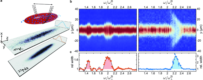
Figure 1: Collective oscillations in a Bose-Fermi mixture. a. Illustration of a Fermi gas (blue) immersed in a Bose-Einstein condensate (red), both trapped in an optical potential. In-situ absorption images of the fermionic ⁴⁰K and bosonic ²³Na are shown beneath. Radial collective oscillations are induced by periodically modulating the depth of the optical potential. b. The doubly integrated line densities along the transverse (y) direction of the boson (left) and fermion (right) clouds as a function of modulation frequency $\omega$, at zero interspecies interaction ($a_{\mathrm{BF}}\,{=}\,0$). c. Spectra of the uncoupled Bose-Fermi system, showing the boson (left, red circles) and fermion (right, blue circles) relative widths, reveal the superfluid hydrodynamic response of the BEC and the response of the non-interacting Fermi gas. The solid black lines show predictions from the hydrodynamic scaling ansatz and a phenomenological Gaussian fit, respectively.

Collective excitations are excellent probes to reveal the role of interparticle scattering. They have been used to demonstrate the superfluid hydrodynamic flow of BECs [57, 58, 59] and collisional hydrodynamics in interacting Fermi gases [60, 61, 62]. Collective oscillations have also been measured in coupled Bose-Fermi superfluids [32, 33, 35, 36] and in Bose-Fermi mixtures [63, 64, 22, 37, 23], revealing phenomena such as the transition between collisionless to collisionally hydrodynamic flow in coupled thermal gases [63], and sound propagation [23]. Here we study a novel regime – the limit of a dilute Fermi gas immersed in a BEC – as relevant for the physics of Bose polarons [38, 39] and unconventional superconductors with low carrier densities [65].

We probe collective excitations of ⁴⁰K fermions and a ²³Na BEC as a function of drive frequency and across a range of Bose-Fermi interactions, revealing the energy and spectral width of low-lying excitations. The experiment starts with an ultracold Fermi gas immersed in the BEC, both held in a $1064\text{\,}\mathrm{nm}$ optical trap with near-cylindrical symmetry (see Fig. 1a). For our coldest samples we evaporatively cool both species to $T{\approx}$ 30 nK, corresponding to $T/T_{\mathrm{c}}\,{\lesssim}\,0.2$, where $T_{\mathrm{c}}$ is the condensate’s critical temperature. Both species are in their respective hyperfine ground state ($\ket{F=1,m_{F}=1}$ for ²³Na and $\ket{F=9/2,m_{F}=-9/2}$ for ⁴⁰K). We control the interspecies interactions by ramping the magnetic field near Feshbach resonances, allowing us to continuously tune the $s$-wave scattering length, $a_{\mathrm{BF}}$. The typical peak boson density is $n_{\mathrm{B}}\,{=}\,7\times 10^{13}$ cm^-3, and the typical fermion impurity concentration is between $n_{\mathrm{F}}/n_{\mathrm{B}}\,{\approx}\,0.003-0.02$.

We characterize the low-energy radial excitations of the mixture at varying interspecies interaction strengths. Modulating the radial trapping potential depth at frequency $\omega$ for 10 cycles, we measure the in situ width of the clouds (see Fig. 1a.) The number of cycles $N$ allows for spectral resolution ${\sim}\,\omega/N$ while the probe time is kept short compared to the mixture’s lifetime. When the modulation excites a resonant mode of either species, the cloud’s width expands radially. Fig. 1b-c depicts the bosonic and fermionic spectrograms for a decoupled mixture at $a_{\rm BF}{=}\,0$. A fermionic resonance is excited at $2\,\omega_{y}^{\text{F}}$, and two resonances of the BEC are apparent at $\sqrt{2}\omega_{\perp}^{\text{B}}$ and $2\omega_{\perp}^{\text{B}}$. Here, $\omega_{y}^{\text{F}}$ is the fermions’ radial trapping frequency, and $\omega^{\mathrm{B}}_{\perp}\,{=}\,(\omega^{\mathrm{B}}_{x}\omega^{\mathrm{B}}_{y})^{1/2}$ is the bosons’ geometric mean radial trapping frequency, with the two frequencies related by $\omega_{y}^{\text{F}}=1.16\,\omega_{\perp}^{\text{B}}$  [66]. The spin-polarized fermions are a collisionless gas [67], which in a purely harmonic trap has its lowest parametric resonance for motion along the y-axis at $2\omega_{y}^{\text{F}}$. The BEC obeys superfluid hydrodynamics, which couples the two collisionless radial modes, giving rise to a quadrupole (out of phase) and a breathing (in phase) resonance at $\sqrt{2}\omega_{\perp}^{\text{B}}$ and $2\omega_{\perp}^{\text{B}}$, respectively [68, 69]. Across all frequencies, the bosonic spectral response is well captured using a hydrodynamic scaling ansatz [70, 66] (see red shaded area in Fig. 1c):

$$\ddot{b}_{i} +{\omega_{i}^{B}}(t)^{2}b_{i}-\frac{{\omega_{i}^{B}}(0)^{2}}{b_{i}\prod_{j}b_{j}}=0$$ (1)

where $i\,{\in}\,(x,y,x)$ and $b_{i}$ is the dimensionless scaling parameter of the BEC’s Thomas-Fermi radius in the $i$-th direction. The energy and spectral width of the fermions’ spectral response is obtained using a fit to a phenomenological function [66] (see Fig. 1c). The broad fan below $2\omega_{y}^{\text{F}}$ visible in the fermionic response (Fig. 1b) arises from strong driving in an anharmonic trap [66].

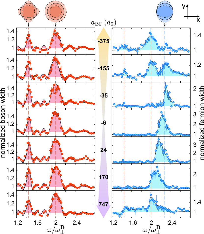
Figure 2: Evolution of Bose-Fermi collective modes across varying interaction strength. Illustrations depict the oscillations of the cloud’s transverse ($x$-$y$) cross-section. The boson quadrupole and breathing modes (shown in red) lie at $\sqrt{2}\omega^{\mathrm{B}}_{\perp}$ and $2\omega^{\mathrm{B}}_{\perp}$, respectively, whereas the fermions’ transverse resonance in the collisionless regime lies at $2\omega^{\mathrm{F}}_{y}$ (shown in blue). The spectra depict bosonic and fermionic cloud widths (circles) for varying modulation frequencies. As $a_{\rm BF}$ increases toward either repulsive or attractive interactions, the fermion spectra evolve to mode lock to the BEC’s superfluid hydrodynamic modes. An extended data set can be found in  [66].

Fig. 2 shows a selection of the bosons’ and fermions’ spectral response for various interspecies coupling strengths. The resonances of the BEC are in all cases well described by the hydrodynamic scaling ansatz from Eq. 1. The BEC spectrogram remains unaffected by the interactions with the fermionic impurities because the Fermi gas is much more dilute. By contrast, the response of the Fermi gas shows a strong dependence on the interspecies coupling strength. At weak couplings, the collisionless mode of the fermions shifts linearly with $a_{\text{BF}}$. With increasing attractive interactions strengths, the fermionic response changes drastically, revealing two additional modes in the their spectral response that coincide with the BEC’s hydrodynamic superfluid modes at $2\omega_{\perp}^{\text{B}}$ and $\sqrt{2}\omega_{\perp}^{\text{B}}$. All three modes are spectrally well resolved and show no broadening beyond the Fourier limit, in contrast to the broadened profiles that would arise from momentum-relaxing collisions [66]. This is remarkable, given that the mean-free path for collisions changes from infinity at zero interaction strength to $l_{\rm mfp}=(4\pi a_{\mathrm{BF}}^{2}n_{\mathrm{B}})^{-1}\,\sim\,0.6\,\mu$m at the strongest measured interactions, so much shorter than the radial system size $L\sim 10\,\mu$m. A thermal mixture would thus cross over from collisionless to collisionally hydrodynamic behavior, through an intermediate regime of strong damping. Here, instead, the fermions continue to flow through the condensate without dissipation, and, for the strongest interactions, even “copy” the BEC’s superfluid collective modes, not unlike dye particles in water.

The fermion collective modes are summarized in Fig. 3. For strong interactions, regardless of their sign ($|a_{\text{BF}}|\,{>}\,350\,a_{0}$, with $a_{0}$ being the Bohr radius), the fermions exclusively respond at the BEC’s hydrodynamic superfluid modes and show no signal of their own collisionless mode. For weaker interactions, we observe a mean-field like shift of the fermion frequency proportional to the sign of the interaction, which for strong repulsive interactions merges with the BEC’s breathing mode at $2\omega_{\perp}^{\text{B}}$ and becomes spectrally indistinguishable. We note that at strong repulsive interactions we observe a dispersive - rather than absorptive - feature in the fermionic response at the BEC quadrupole mode (Fig. 2). This Fano-type behavior can be understood from coherent coupling of the fermionic and bosonic mode [71].

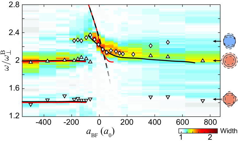
Figure 3: Fermionic mode frequencies versus interspecies interaction. The color density plot displays the power spectra of cloud widths. White markers denote the peak frequencies. The arrows on the right side indicate the three modes of Fig. 2. The dashed line shows the naive mean-field prediction, and the red line is the scaling ansatz solution of the mean-field model. The black lines show the dominant modes of the Boltzmann-Vlasov solution accounting for finite system size and trap anharmonicity [66].

To understand the dynamics across all interaction strengths, we compare various numerical models to the data. The linear dependence of the fermionic collisionless mode at weak interaction strengths qualitatively agrees with a mean-field description, considering the effective potential experienced by the fermions immersed in the Bose gas. The BEC in the Thomas-Fermi approximation takes on the shape of the inverted optical potential. The fermions thus experience a joint effective potential comprising the optical trap and the mean-field potential of the BEC, where attractive (repulsive) interspecies interactions provide a steeper (shallower) potential that shifts the trapping frequencies according to $\tilde{\omega}^{2}{=}\,{\omega^{F}_{y}}^{2}\left(1\,{-}\,\frac{g_{\rm BF}\alpha_{\rm B}}{g_{\rm BB}\alpha_{\rm F}}\right)$ [66]. Here, $g_{\mathrm{BF}}\,{=}\,2\pi\hbar^{2}a_{\mathrm{BF}}/\mu$ is the Bose-Fermi coupling strength, $\mu\,{=}\,m_{\mathrm{F}}m_{\mathrm{B}}/(m_{\mathrm{F}}+m_{\mathrm{B}})$ is the reduced mass, $g_{\mathrm{BB}}\,{=}\,4\pi\hbar^{2}a_{\mathrm{BB}}/m_{\mathrm{B}}$ is the Bose-Bose coupling, and $\alpha_{\rm B(F)}$ is the boson (fermion) optical polarizability. Qualitatively, this mean-field model (black dashed line in Fig. 3) shares the trend of the measurements for small $a_{\text{BF}}$, but with a different slope $\omega$ versus $a_{\rm BF}$. It also fails to predict the appearance of additional modes in the fermionic spectral response. To capture the resonances that fermions inherit from the BEC’s superfluid hydrodynamic modes, the mean-field potential itself must properly incorporate the bosons’ response given by the scaling ansatz Eq. 1.

We therefore turn to the full dynamics of the fermions as described by the Boltzmann-Vlasov equation,

$$\frac{\partial f}{\partial t}+\frac{d\textbf{r}}{dt}\frac{\partial f}{\partial\textbf{r}}+\frac{d\textbf{p}}{dt}\frac{\partial f}{\partial\textbf{p}}=I_{\rm coll}$$ (2)

where $f$ is the fermion distribution at momentum p and position r, and $I_{\rm coll}$ is the collision integral. Anticipating the absence of collisions for fermions only interacting with the BEC, in the absence of thermal excitations, we may set $I_{\rm coll}=0$. Then, to first order in $g_{\rm BF}$, we derive a scaling ansatz for the fermions’ width, assuming a harmonic trap and fermionic impurities that are deeply immersed in the BEC [70, 72, 47]:

$$\ddot{c}_{i} +{{\omega^{F}_{\rm i,eff}}}(t)^{2}c_{i}-\left(1-\frac{g_{\rm BF}\alpha_{\rm B}}{g_{\rm BB}\alpha_{\rm F}}\right)\frac{{\omega^{F}_{y}}(0)^{2}}{c_{i}^{3}}=0$$

$${\mathrm{with~{}}{\omega^{F}_{\rm i,eff}}} (t)^{2}=\left(1-\frac{g_{\rm BF}\alpha_{\rm B}}{g_{\rm BB}\alpha_{\rm F}}\right){\omega^{F}_{i}}(t)^{2}-\frac{g_{\rm BF}}{g_{\rm BB}}\frac{\ddot{b_{i}}}{b_{i}}$$ (3)

Here, $c_{i}$ is the dimensionless scaling parameter of the width of the Fermi gas, with $c_{i}(t{=}0)\,{=}\,1$. This ansatz captures the fermionic response to the BEC’s superfluid mode on the attractive side [66], which can thus indeed be explained as the dissipationless flow of fermions experiencing the coherent interactions with the BEC. The simple ansatz fails for repulsive interactions above $a_{\text{BF}}\,{>}\,100\,a_{0}$ where the mean-field potential is strong enough to repel fermions from the BEC. A full numerical simulation of the dissipationless Boltzmann-Vlasov equation [66] – including the temperature-dependent fermionic cloud size and the trap anharmonicity – is shown as the black solid line in Fig. 3, which accurately captures all of the observed modes across all interaction strengths, validating our neglect of the collisional term in Eq. 2.

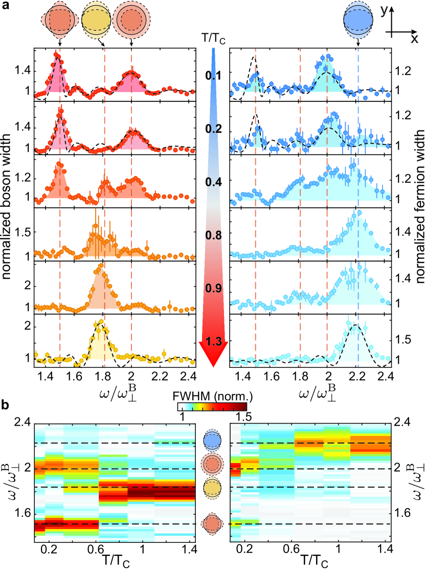
Figure 4: Temperature dependence of the bosonic and fermionic collective modes at $\mathbf{a_{\mathrm{BF}}\,{=}\,{-}400a_{0}}$. a. Spectrograms of the boson (left) and fermion (right) widths, as a function of the bosons’ reduced temperature $T/T_{\mathrm{c}}$. Top cartoons illustrate the bosonic hydrodynamic (red), collisionless (yellow), and the fermionic collisionless (blue) modes. Peak boson densities for increasing $T/T_{\mathrm{c}}$ are $n_{\rm B}{=}(7.3,5.9,5.4,2.3,1.4,0.07){\times}10^{13}$ cm^-3, respectively. The fermion spectrograms indicate hydrodynamic response at the BEC’s quadrupole and breathing mode frequencies for the lowest temperatures. Dashed lines in the upmost panels for $T/T_{\mathrm{c}}\approx 0.1$ and $T/T_{\mathrm{c}}\approx 0.2$ represent the theoretical prediction based on the scaling ansatz for the BEC dynamics and Boltzmann-Vlasov equation for the dynamics of fermions. Dashed lines for $T>T_{\mathrm{c}}$ show the result of solving coupled Bose-Fermi Boltzmann equations [66]. b. Summary of the obtained peak frequencies for bosons (left) and fermions (right), with color indicating spectral response.

Indeed, dissipationless flow is expected for the Fermi gas well below the bosons’ superfluid transition temperature, as fermions slower than the condensate’s speed of sound ($\sim\,5\mu$m/ms) can only dissipate energy through collisions with thermal bosons, which are essentially absent at low temperatures $T/T_{\mathrm{c}}\approx 0.2$. To measure the impact of collisions of fermions with thermal bosons, we now probe the mixture at increasing temperatures across the BEC phase transition. The physics is complex already for bosons alone, as the BEC becomes immersed in a cloud of thermal excitations, and the thermal cloud’s collective modes couple to the superfluid modes [69]. We employ the same protocol as before, using a drive that couples strongly to the BEC’s quadrupole mode [66]. The relative temperature $T/T_{\mathrm{c}}$ is varied at a fixed interaction strength by reducing the number of bosons while fixing the same final temperature. The radial trap ellipticity [66] allows us to distinguish the collisionless mode of the bosons’ thermal component at $2\omega_{y}^{\text{B}}$ from the superfluid breathing mode at $2\omega_{\perp}^{\text{B}}$, as depicted in Fig. 4a. Fig. 4b displays the change of the bosons’ and fermions’ spectral responses with temperature. At low temperatures, the bosons exhibit resonances at the BEC quadrupole ($\sqrt{2}\omega^{\mathrm{B}}_{\perp}$) and breathing ($2\omega^{\mathrm{B}}_{\perp}$) modes. At $T\,{>}\,0.5\,T_{\mathrm{c}}$ we observe an additional peak at $2\omega_{y}^{\text{B}}$, corresponding to the intraspecies collisionless mode of the bosonic thermal component [58, 57]. With increasing $T/T_{\mathrm{c}}$ the bosonic response at the BEC superfluid modes is reduced while the response at the intraspecies collisionless mode grows, until above $T_{\mathrm{c}}$ only the collisionless mode persists.

The fermions can be viewed as a highly sensitive probe for the complex crossover of modes in the Bose gas. At the coldest temperatures, they respond exclusively at the frequencies of the BEC’s hydrodynamic modes, giving rise to the dissipationless flow. Remarkably, starting at $T/T_{\mathrm{c}}\,{\approx}\,0.4$, two additional modes appear in the fermionic response. The lower resonance at $2\omega^{\mathrm{B}}_{y}$ coincides with the intraspecies collisionless mode of the bosonic thermal component whereas the higher one at $2\omega^{\mathrm{F}}_{y}$ coincides with the native collisionless mode of the fermions. Above $T_{\mathrm{c}}$, the fermions respond only at their collisionless mode at $2\omega^{\mathrm{F}}_{y}$, and this regime is well captured by solving the full coupled Boltzmann equations for the mixture with nonvanishing $I_{\rm coll}$ [66, 71]. We note that while the thermal components of the bosons and the spin-polarized fermions are both in the collisionless regime by themselves, strong interspecies interactions bring this mixture into local equilibrium [63]. We interpret the fermionic response at the bosonic collisionless mode ($0.3\,T_{\rm c}\lesssim T\lesssim T_{\rm c}$) as an indication of the mixture’s crossover from the collisionless to the collisionally hydrodynamic regime. Above $T_{\mathrm{c}}$, the mixture reverts to collisionless flow for both species due to the lowered density of bosons.

Our results demonstrate dissipationless flow of fermions immersed in a Bose condensate, i.e. the absence of momentum-changing collisions even for strong interspecies interactions. As the temperature is increased, incoherent collisions between the thermal bosons and fermions cause a crossover into the collision-dominated hydrodynamic regime, in direct analogy to 2D electron gases, where the electron mean-free path is tuned with the density and temperature. At temperatures lower than those achieved in this study, induced fermion-fermion interactions [73, 74] are predicted to arise within the Bose-Fermi mixture, a precursor of the long-sought $p$-wave superfluidity of fermions mediated by bosons [75, 76, 77].

Acknowledgements: We acknowledge Eric Wolf for helpful discussions. This work was supported by the NSF, AFOSR, ARO, AFOSR MURI on “Exotic Phases of Matter,” the David and Lucile Packard Foundation, the Vannevar Bush Faculty Fellowship, and the Gordon and Betty Moore Foundation through grant GBMF5279. Z. Z. Y. and A. C. acknowledge support from the NSF GRFP. C. R. acknowledges support from the Deutsche Forschungsgemeinschaft (DFG) Germany research fellowship (421987027). K. S. acknowledges funding from NSF EAGER-QAC-QCH award No. 2037687. P. D. and E. D. were supported by ARO grant number W911NF-20-1-0163, the SNSF project 200021-212899. E. D. acknowledges support from the Swiss National Science Foundation under Division II.

Supplemental Information

1 Methods

Here we describe details of the collective oscillation measurements. The optical potential is approximately cylindrically symmetric with trap frequencies of $\omega^{\mathrm{B}}_{x,y,z}/2\pi{=}[103(3),94(2),12.2(0.3)]\,$Hz and $\omega^{\mathrm{F}}_{x,y,z}/2\pi{=}[125(2),114(2),15(1)]$ Hz for bosons and fermions. The fermions are moderately degenerate with $T/T_{\mathrm{F}}$ ranging from 0.6 to 2, where $T_{\mathrm{F}}$ is the Fermi temperature. The BEC is weakly interacting with a Bose-Bose scattering length of $a_{\rm BB}\,{=}\,52\,a_{0}$, where $a_{\text{0}}$ is the Bohr radius. Our lowest temperatures are $T/T_{\mathrm{c}}\,{\lesssim}\,0.2$ with respect to the BEC critical temperature $T_{\mathrm{c}}$. To create an interacting Bose-Fermi mixture, we ramp the magnetic field in between two interspecies Feshbach resonances, allowing continuous tuning of the interspecies $s$-wave scattering length, $a_{\mathrm{BF}}$.

We study the collective modes versus interaction strength at a fixed $T/T_{\mathrm{C}}\,{\approx}\,0.2$ (see main text Fig. 2) by applying a sinusoidal intensity perturbation on the $z$-axis $1064\text{\,}\mathrm{nm}$ trap beam with a modulation amplitude of 20% and a variable drive frequency. This method primarily excites the transverse breathing mode. We study the collective modes versus temperature at a fixed interaction strength (set by the scattering length $a_{\rm BF}\,{=}\,-400\,a_{0}$) by applying intensity modulations to both the $z$- and $y$-directional $1064\text{\,}\mathrm{nm}$ beams (see main text Fig. 4). The modulation in each direction is $180^{\circ}$ out of phase in order to better couple to the transverse quadrupole mode. The modulation depths are 15% for both beams. In both cases, the clouds are imaged after a duration lasting ten oscillation cycles.

Fitting of the fermion spectrograms, i.e. in Fig. 1 of the main text, is performed with a phenomenological asymmetric function of the form

$$c(\omega,p_{i})=\frac{p_{1}}{f(\omega,p_{2},p_{3},p_{4})} e^{-(\omega-p_{2})^{2}/f(p_{2},p_{3},p_{4})^{2}}$$

$$\text{with}~{}f(\omega,p_{2},p_{3},p_{4}) =p_{3}(1+e^{p_{4}(\omega-p_{2})})^{-1}$$ (S1)

with $p_{i}$ as free fitting parameters. This function reduces to a Gaussian in the limit $p_{4}\,{=}\,0$, and only the peak location and width are used in data analysis. The asymmetry is due to strong driving of the fermions in an anharmonic trap.

In Fig. 1-4 of the main text, the modulation frequencies are shown as normalized to the boson mean radial trap frequency, $\omega_{\perp}^{\rm B}$, which is $2\pi\times$ 98 Hz on average. However, long-term drifts of the trap depth over many experimental repetitions necessitated a different normalization for each interaction strength in Fig. 2-3. The exact normalization value was determined by fitting a Gaussian to the boson spectrograms at frequencies near $\omega_{\perp}^{\rm B}$, extracting the frequency of the largest response, and assigning that as the normalization for the boson and fermion spectograms for that particular $a_{\rm BF}$. This procedure necessarily forces the BEC breathing mode in Fig. 2 to fall at $2\omega_{\perp}^{\rm B}$, and falls to the same absolute frequency to within 2% error for all driving conditions.

2 Boson hydrodynamic collective modes at $T=0$

To understand the collective modes of the majority bosons, we utilize the approach of [70] based on a scaling ansatz. For BECs in a time-dependent harmonic potential, the spatial density evolves as a dilation, characterized by $x$-,$y$-, and $z$-scaling factors $\lambda_{j}(t)$ that satisfy

$$\ddot{\lambda}_{i} +\omega_{i}^{2}(t)\lambda_{i}-\frac{\omega_{i}^{2}(0)}{\lambda_{i}\prod_{j}\lambda_{j}}=0$$ (S2)

$$\omega^{2}_{x}(t) =\omega^{2}_{x}(0)\big{(}1+f\alpha_{2}\sin(\omega_{\mathrm{mod}}t)$$

$$+(1-f)\alpha_{1}\sin(\omega_{\rm mod}t+\phi_{1})\big{)}$$

$$\omega_{y}^{2}(t) =\omega_{y}^{2}(0)\big{(}1+\alpha_{2}\sin(\omega_{\mathrm{mod}}t)\big{)}$$

$$\omega_{z}^{2}(t) =\omega_{z}^{2}(0)\big{(}1+\alpha_{1}\sin(\omega_{\mathrm{mod}}t+\phi_{1})\big{)}$$

for $j=\{x,y,z\}$. Here, $f$ depends on the trapping geometry and was taken as a fitting parameter for the data in main text Fig. 2a, held constant over all $a_{\rm BF}$. $\alpha_{1},\alpha_{2}$ are the modulation amplitudes and $\phi_{1}$ is the relative phase shift. Numerical solutions to these equations are shown in the boson spectra of Fig. 1 and 2 of the main text.

3 Mean field shift of fermion collective mode

For weak interactions and small perturbations, a single fermion impurity feels a combined potential from the optical trap and the mean-field energy of the bosons. Its trapping frequency is shifted from the interaction-free frequency $\omega_{i}$ by

$$\tilde{\omega}^{2}_{i}=\omega^{2}_{i}\left(1-\frac{g_{\mathrm{BF}}\alpha_{\mathrm{B}}}{g_{\mathrm{BB}}\alpha_{\mathrm{F}}}\right)$$ (S3)

where, $g_{\mathrm{BF}}\,{=}\,2\pi\hbar^{2}a_{\mathrm{BF}}/\mu$ is the Bose-Fermi coupling, $\mu\,{=}\,m_{\mathrm{B}}m_{\mathrm{F}}/(m_{\mathrm{B}}+m_{\mathrm{F}})$ is the reduced mass, $g_{\mathrm{BB}}\,{=}\,4\pi\hbar^{2}a_{\mathrm{BB}}/m_{\mathrm{B}}$ is the Bose-Bose coupling, and $\alpha_{\mathrm{B(F)}}$ is the boson’s (fermion’s) optical polarizability. Physically, this represents the fermion seeing an effectively higher potential when attracted to the boson reservoir, which occupies the bottom of the optical trap, and vice versa for repulsive interactions. As can be seen in the dashed black line of Fig. 3 of the main text, Eq. S3 qualitatively captures the trend of the breathing response in the weak-interaction regime but overpredicts the magnitude of the trend. The deviation arises because of anharmonicity and because the Fermi cloud has a similar width compared to the boson size, overlapping with regions of zero condensate density, thereby invalidating the assumption of Eq. S3.

Therefore we employ a model that takes into account the equilibrium atom distributions. The fermions are given by a Maxwell-Boltzmann distribution at $T{=}80$ nK, initially in equilibrium in the optical potential with $U_{\rm ODT}(y)=-U_{0}e^{-\frac{2y^{2}}{w^{2}}}$, where the trap depth is $U_{0}=h\times 155$ kHz and the waist is 110$\,\mu$m. The bosons are described by a zero-temperature Thomas-Fermi (TF) approximation [69].

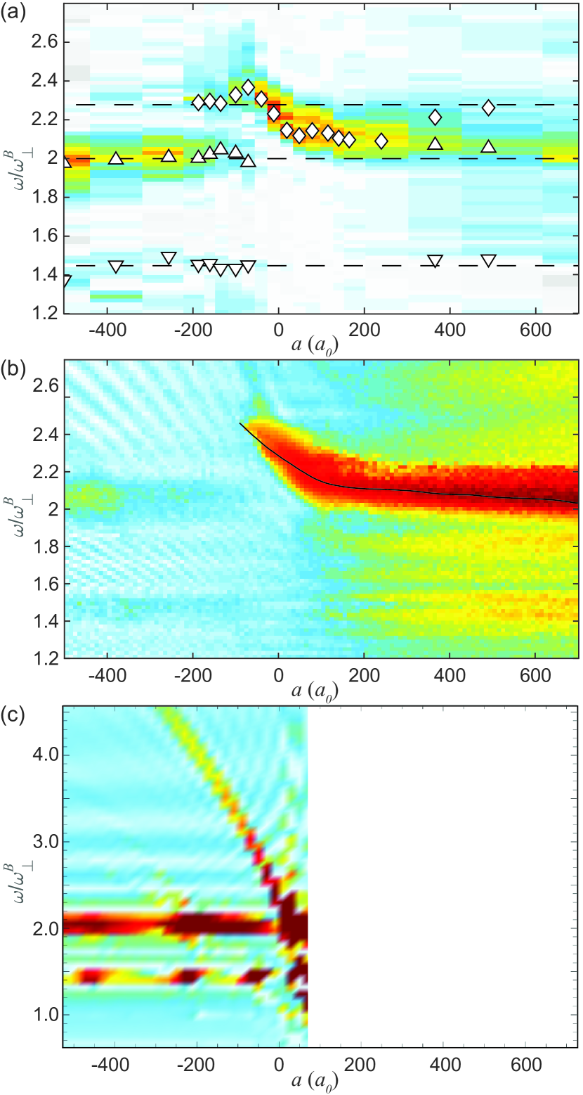
Figure S1: Spectra of fermion widths at various interaction strengths, comparing (a) the experiment to (b) the simulation of the Boltzmann mean field model with a Gaussian trapping potential and finite-sized BEC, as described in the text. The color density plot shows the power spectra of fermion widths relative to their equilibrium widths. (c) The solution of the Boltzmann mean field model using the scaling ansatz, as captured in Eq. S9. This solution is only valid for $g_{\rm BF}\alpha_{B}/g_{\rm BB}\alpha_{F}<1$. All spectra neglect the presence of thermal bosons.

The fermion trajectories are solved numerically from the Boltzmann equation with zero collisions.

$$\frac{\partial f}{\partial t}+\sum_{i}v_{i}\frac{\partial f}{\partial x_{i}}-\frac{1}{m}\frac{dU}{dx_{i}}\frac{\partial f}{\partial v_{i}} =0$$ (S4)

Here, $U(\mathbf{x},t)=U_{\rm trap}(\mathbf{x},t)+U_{mf}(\mathbf{x},t)$, where the mean-field potential is $g_{\mathrm{BF}}n_{\mathrm{B}}(\mathbf{x},t)$. Results of the numerical simulation are shown in Fig. S1(b), accurately reproducing the features of the data, and shown in Fig. S1(a).

Finally, we can derive a simple solution to Eq. S4 using a scaling ansatz, as employed by [70, 72, 47]. Here we neglect the anharmonicity of the trap as well as the possibility that the fermions leave the BEC spatial region. Let $b_{i}\,(c_{i})$ be the dimensionless scaling parameter for the boson Thomas-Fermi radius (fermion Gaussian width) in the $i$th direction, $x_{\mathrm{TF,i}}$. Without interactions, both species admit scaling solutions:

$$\ddot{b}_{i}+\omega_{iB}^{2}(t)b_{i}-\frac{\omega_{iB}^{2}(0)}{b_{i}\prod_{j}b_{j}} =0$$ (S5)

$$\ddot{c}_{i}+\omega_{i}^{2}(t)c_{i}-\frac{\omega_{i}^{2}(0)}{c_{i}^{3}} =0.$$ (S6)

for bosons and fermions, respectively. This simple scaling is no longer satisfied in the case of a finite Bose-Fermi (BF) interaction, but is still a useful approximation to first order in $g_{\mathrm{BF}}$. The BF interaction adds terms of the following form to Eq. S6

$$-\frac{c_{i}}{mx_{i}}\partial_{x_{i}}(g_{\mathrm{BF}}n_{\mathrm{B}}) =$$ (S7)

$$\frac{c_{i}~{}g_{\mathrm{BF}}~{}\omega_{iB}^{2}(0)}{g_{\mathrm{BB}}~{}\Pi_{j}b_{j}b_{i}^{2}}.$$ (S8)

With appropriate substitutions, the scaling solution can therefore be approximated as

$$\ddot{c}_{i}+{{\omega^{F}_{\rm i,eff}}}(t)^{2}c_{i} -\left(1-\frac{g_{\rm BF}\alpha_{\rm B}}{g_{\rm BB}\alpha_{\rm F}}\right)\frac{{\omega^{F}_{y}}(0)^{2}}{c_{i}^{3}}=0$$

$${\mathrm{with~{}}{\omega^{F}_{\rm i,eff}}}(t)^{2} =\left(1-\frac{g_{\rm BF}\alpha_{\rm B}}{g_{\rm BB}\alpha_{\rm F}}\right){\omega^{F}_{i}}(t)^{2}-\frac{g_{\rm BF}}{g_{\rm BB}}\frac{\ddot{b_{i}}}{b_{i}}$$ (S9)

for small displacements within the BEC TF radius. This equation describes a harmonic oscillator driven by both the direct variation of the fermion frequency and by the changing condensate shape. As such, one observes resonances, apart from the mean-field solution, also where the BEC is strongly modulated. These resonances couple strongly when they equal an integer fraction of the dressed fermion frequency (see Fig. S1c).

4 Equilibrium line densities of the Bose-Fermi mixture

We report the equilibrium distributions of the Bose-Fermi mixture across different interaction strengths and temperatures. Fig. S2 shows the line densities of the fermions in the $y$- and $z$- directions, obtained by integrating the absorption image in the $x$ and $y$ directions, respectively. These examples were taken at a modulation frequency that was not resonant for any interaction strength. Therefore, they represent the equilibrium distribution of the fermions prior to any excitations. Fig. S3 shows the line densities of the equilibrium Bose-Fermi mixture corresponding to the data shown in Fig. 4 of the main text.

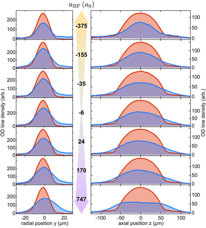
Figure S2: Equilibrium line density distributions for the fermions versus interaction strength. Line densities showing the optical density versus position for the fermions (in blue) and the bosons (in red), for the $y$- and $z$- directions.

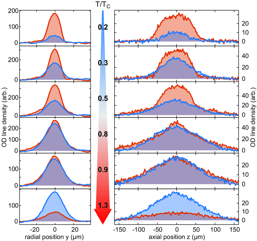
Figure S3: Equilibrium line density distributions for the fermions versus reduced temperature. Line densities showing the optical density versus position for the fermions (in blue) and the bosons (in red), for the $y$- and $z$- directions.

5 Collective oscillations in the time domain

The collective oscillations can also be studied in the time domain rather than in the frequency domain, revealing coherent, in-phase oscillations between the bosons and fermions when interactions are tuned to where the fermions respond to the superfluid bosons’ hydrodynamic modes. Fig. S4 shows the evolution of the cloud size versus time, revealing how the fermion cloud width follows the bosonic behavior across multiple cycles without apparent damping or dephasing. Both clouds oscillate at the boson breathing mode near $2\omega^{B}_{\perp}$.

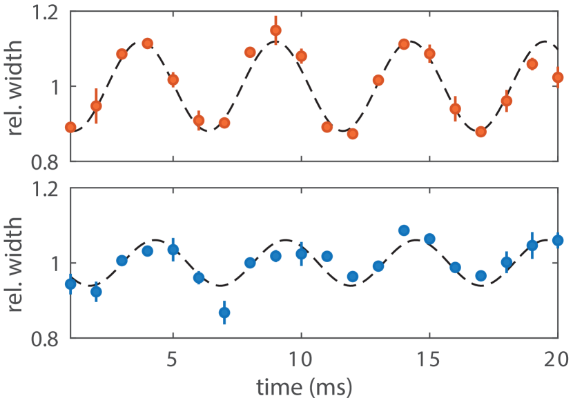
Figure S4: Evolution of cloud size versus time. Collective oscillations of transverse width of bosons (top) and fermions (bottom) in the hydrodynamic regime. The traces were taken at a modulation frequency of $\omega\,{=}\,1.93\,\omega^{B}_{\perp}$ at an interaction strength of $a_{\rm BF}=-250\,a_{0}$. The oscillation was excited by modulating the $x$-direction ODT intensity at 5% for ten cycles. The transverse $y$- widths are shown relative to the equilibrium widths as a function of time. Dashed lines are sinusoidal fits to the data, with the fitted frequencies to the bosons and fermions as $1.9(1)$ and $2.0(1)\,\omega^{B}_{\perp}$, respectively.

6 Evolution of collective modes with temperature

Upon tuning the temperature $T$ at $a_{\rm BF}=-400\,a_{0}$, the experimental data in Fig. 4 of the main text exhibits three regimes that we discuss here in greater detail.

At the lowest temperatures $T\lesssim 0.2\,T_{\rm c}$, the thermal cloud of normal bosons is suppressed, and, as such, the bosonic response to trap perturbations is fully characterized by the superfluid hydrodynamics of the BEC. It is noteworthy that in our discussion of the bosonic response, we neglect the fermions as the fermionic density is at least two orders of magnitude smaller compared to the bosonic density. As mentioned above, the BEC’s evolution is well captured by the scaling ansatz. At the same time, the dynamics of fermions follow the Boltzmann-Vlasov equation, where the BEC enters as a time-dependent mean-field potential and the incoherent collisions are suppressed. Our findings, both in Fig. 3 and Fig. 4 of the main text, indicate that this combined approach captures well the frequencies and lifetimes of the collective modes of the mixture. One discrepancy between this theory and the experiment is that the fermionic amplitudes (for instance, of the quadrupole mode response) are slightly different – this perhaps indicates that the quantum aspects of the Bose polaron dynamics are important to describe the full fermionic response. Based on this discussion, the intrinsic collective response of the mixture at the lowest temperatures is therefore coherent and obeys superfluid hydrodynamics.

Above $T_{\rm c}$, the analysis is also simplified as the bosons behave as a weakly interacting thermal gas. The dynamics of the mixture is then expected to be governed by the coupled Boltzmann equations for the bosonic $n_{\rm B}(\bm{p},\bm{r},t)$ and fermionic $n_{\rm F}(\bm{p},\bm{r},t)$ distribution functions:

$$\Big{(}\partial_{t}+\frac{\bm{p}}{m_{\rm B}}\cdot\partial_{\bm{r}}-\partial_{\bm{r}}U_{\rm eff,B}\cdot\partial_{\bm{p}}\Big{)}n_{\rm B}=I_{\rm BB}+I_{\rm BF},$$ (S10)

$$\Big{(}\partial_{t}+\frac{\bm{p}}{m_{\rm F}}\cdot\partial_{\bm{r}}-\partial_{\bm{r}}U_{\rm eff,F}\cdot\partial_{\bm{p}}\Big{)}n_{\rm F}=I_{\rm FB}.$$ (S11)

For the left-hand sides, we assume the Hartree-Fock approximation:

$$U_{\rm eff,B}=U_{\rm trap,B}+2g_{\rm B}n_{\rm B}(\bm{r},t)+g_{\rm BF}n_{\rm F}(\bm{r},t),$$ (S12)

$$U_{\rm eff,F}=U_{\rm trap,F}+g_{\rm BF}n_{\rm B}(\bm{r},t),$$ (S13)

where $n_{\rm B/F}(\bm{r},t)=\displaystyle\int\frac{d^{3}\bm{p}}{(2\pi)^{3}}n_{\rm B/F}(\bm{p},\bm{r},t)$ represents the bosonic/fermionic real-space density. One can neglect the fermionic density in the effective potentials since it is significantly lower than the bosonic density. At temperatures above $T_{\rm c}$, one is required to take into account the Bose-Bose, Bose-Fermi, and Fermi-Bose collision integrals that read:

$$I_{\rm BB}(\bm{p},\bm{r},t) =2g_{\rm B}^{2}\int\frac{d^{3}\bm{p}^{\prime}}{(2\pi)^{3}}\frac{d^{3}\bm{p}_{1}}{(2\pi)^{3}}\frac{d^{3}\bm{p}^{\prime}_{1}}{(2\pi)^{3}}\times(2\pi)^{3}\delta(\bm{p}+\bm{p}^{\prime}-\bm{p}_{1}-\bm{p}_{1}^{\prime})\times(2\pi)\delta(\varepsilon_{\rm B}(\bm{p})+\varepsilon_{\rm B}(\bm{p}^{\prime})-\varepsilon_{\rm B}(\bm{p}_{1})-\varepsilon_{\rm B}(\bm{p}_{1}^{\prime}))$$

$$\qquad\qquad\qquad\times[(1+n_{\rm B}(\bm{p}))(1+n_{\rm B}(\bm{p}^{\prime}))n_{\rm B}(\bm{p}_{1})n_{\rm B}(\bm{p}_{1}^{\prime})-n_{\rm B}(\bm{p})n_{\rm B}(\bm{p}^{\prime})(1+n_{\rm B}(\bm{p}_{1}))(1+n_{\rm B}(\bm{p}_{1}^{\prime}))],$$ (S14)

$$I_{\rm BF}(\bm{p},\bm{r},t) =g_{\rm BF}^{2}\int\frac{d^{3}\bm{p}^{\prime}}{(2\pi)^{3}}\frac{d^{3}\bm{p}_{1}}{(2\pi)^{3}}\frac{d^{3}\bm{p}^{\prime}_{1}}{(2\pi)^{3}}\times(2\pi)^{3}\delta(\bm{p}+\bm{p}^{\prime}-\bm{p}_{1}-\bm{p}_{1}^{\prime})\times(2\pi)\delta(\varepsilon_{\rm B}(\bm{p})+\varepsilon_{\rm F}(\bm{p}^{\prime})-\varepsilon_{\rm B}(\bm{p}_{1})-\varepsilon_{\rm F}(\bm{p}_{1}^{\prime}))$$

$$\qquad\qquad\qquad\times[(1+n_{\rm B}(\bm{p}))(1-n_{\rm F}(\bm{p}^{\prime}))n_{\rm B}(\bm{p}_{1})n_{\rm F}(\bm{p}_{1}^{\prime})-n_{\rm B}(\bm{p})n_{\rm F}(\bm{p}^{\prime})(1+n_{\rm B}(\bm{p}_{1}))(1-n_{\rm F}(\bm{p}_{1}^{\prime}))],$$ (S15)

$$I_{\rm FB}(\bm{p},\bm{r},t) =g_{\rm BF}^{2}\int\frac{d^{3}\bm{p}^{\prime}}{(2\pi)^{3}}\frac{d^{3}\bm{p}_{1}}{(2\pi)^{3}}\frac{d^{3}\bm{p}^{\prime}_{1}}{(2\pi)^{3}}\times(2\pi)^{3}\delta(\bm{p}+\bm{p}^{\prime}-\bm{p}_{1}-\bm{p}_{1}^{\prime})\times(2\pi)\delta(\varepsilon_{\rm F}(\bm{p})+\varepsilon_{\rm B}(\bm{p}^{\prime})-\varepsilon_{\rm F}(\bm{p}_{1})-\varepsilon_{\rm B}(\bm{p}_{1}^{\prime}))$$

$$\qquad\qquad\qquad\times[(1-n_{\rm F}(\bm{p}))(1+n_{\rm B}(\bm{p}^{\prime}))n_{\rm F}(\bm{p}_{1})n_{\rm B}(\bm{p}_{1}^{\prime})-n_{\rm F}(\bm{p})n_{\rm B}(\bm{p}^{\prime})(1-n_{\rm F}(\bm{p}_{1}))(1+n_{\rm B}(\bm{p}_{1}^{\prime}))],$$ (S16)

where $\varepsilon_{\rm B/F}(\bm{p})=p^{2}/(2m_{\rm B/F})$.

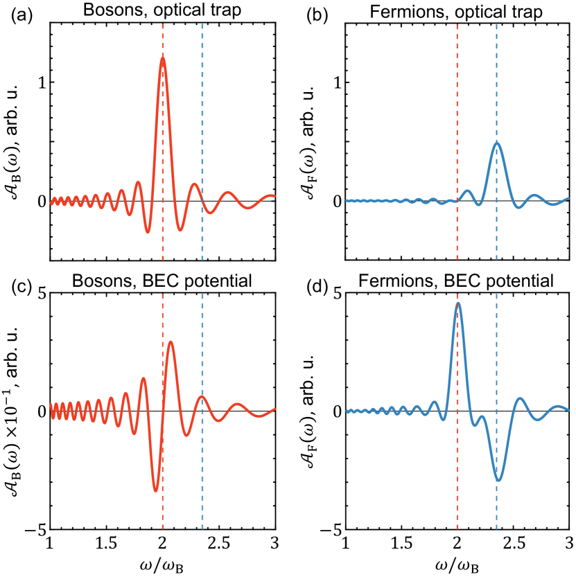
Figure S5: Thermal cloud responses at $T/T_{\rm c}=0.9$. Here the modulation of the optical trap, the observables, and the choice of the simulation parameters follow the experiment (see text). The bosonic thermal cloud response (a) exhibits a peak at $2\omega_{\rm B}$, while the fermionic one (b) at $2\omega_{\rm F}$. Besides, the fermions exhibit a weak feature at $2\omega_{\rm B}$ indicating they are sensitive to the bosonic collective modes. The trap modulation also perturbs the BEC, which in turn then gives an additional drive to the two thermal clouds via the time-dependent mean-field potentials. (c) and (d) show the resulting responses to this perturbation. In particular, the bosons (c) show a notable enhancement at $2\omega_{\rm B}$, as in our modeling, the BEC gives rise to a resonant driving of the bosonic cloud. The fermions (d) now also exhibit much stronger peak at $2\omega_{\rm B}$ – this contribution comes from both the BEC oscillations and from the resonantly driven thermal bosonic cloud.

One can then analyze collective modes, and linear response of the mixture in general, using the method-of-moments (for specific examples of this approach we refer the reader to Refs. [78, 79]). In particular, we first linearize the above equations of motion on top of the equilibrium state: $n_{\rm B/F}(\bm{r},\bm{p},t)=n_{\rm B/F,\rm eq}(\bm{r},\bm{p})+\Delta_{\rm B/F}(\bm{r},\bm{p})\Phi_{\rm B/F}(\bm{r},\bm{p},t)$, where $\Delta_{\rm B/F}(\bm{r},\bm{p})=n_{\rm B/F,\rm eq}(\bm{r},\bm{p})[1\pm n_{\rm B/F,\rm eq}(\bm{r},\bm{p})]$. We then expand the small fluctuations $\Phi_{\rm B/F}(\bm{r},\bm{p},t)$ in some suitable basis set, which in turn reduces the infinite-dimensional linear problem to a finite-dimensional matrix equation. By solving this equation numerically, one obtains linear response properties of the mixture and, thus, can compare this theory and the experiment. Because of the complexity of the collision integrals, the actual calculations are tedious and, for this reason, relegated to a separate manuscript [71] – below we simply outline the results of such an analysis. In our analysis we also neglect the small transverse asymmetry of the traps and focus only on the monopole breathing mode that is now decoupled from the quadrupole one. As indicated in the bottom panels of Fig. 4b of the main text, this approach gives an excellent agreement with the experiment. Because the bosonic density above $T_{\rm c}$ in the experiment is relatively small, the intrinsic dynamics we observe above $T_{\rm c}$ are best described as collisionless. Indeed, we find that the bosonic response peaks at $2\omega_{\rm B}$, while the fermionic one is at $2\omega_{\rm F}$, and the two quantities seem to be decoupled from each other. A signature of a collision-dominated regime would be if either of these responses exhibited a notable admixture of both bosonic and fermionic resonances – this situation is expected to emerge for larger bosonic densities [71].

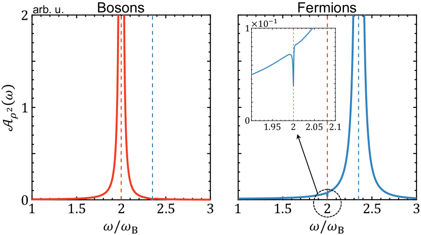
Figure S6: Thermal cloud responses at $T/T_{\rm c}=1.3$ to a broadband optical quench. Here we plot slightly different quantities than in Fig. S5, namely: the bosonic and fermionic spectral functions ${\cal A}_{\rho^{2}}(\omega)$ encode the time-dependent changes of the transverse cloud sizes to a $\delta(t)$-like modulations of the transverse optical traps. The bosonic response (left) exhibits a resonance at $2\omega_{\rm B}$, while the fermions (right) are peaked at $2\omega_{\rm F}$. The inset shows that the fermionic response shows a weak feature at $2\omega_{\rm B}$, indicating that the fermions can be viewed as a sensor of the bosonic subsystem.

The most challenging, yet perhaps the most interesting regime is when $0.3T_{\rm c}\lesssim T\lesssim T_{\rm c}$. We point out that a theory for this situation is not yet even fully established. Nonetheless, we can combine the low and high temperature approaches to attempt to understand the intermediate temperatures. In this intermediate temperature regime, both the BEC and the bosonic thermal cloud are important. As for the case of the lowest temperatures, we approximate the BEC dynamics within the scaling ansatz. Similar to the case of high temperatures, we take into account the collision processes and describe the mixture of the thermal bosons and fermions within the Boltzmann framework. The BEC creates time-dependent Vlasov-like potentials to the thermal clouds, but we neglect the back-action from the clouds to the condensate dynamics; in particular, we neglect incoherent scatterings off the condensate. In other words, the BEC learns about the normal bosons only at the level of the equilibrium wave function that is still well-described within the Thomas-Fermi approximation.

Figure S5 summarizes the results of this approach. The response of either of the thermal clouds can be viewed as a sum of two terms – the first term comes from the direct optical driving of the trap potentials; the second one is due to the time-dependent BEC, which actually also acquires its dynamics through this trap modulation. As shown in Fig. S5a,b, the first term results in responses similar to the ones we had for $T>T_{\rm c}$, i.e., the bosonic cloud exhibits a peak at $2\omega_{\rm B}$, while the fermionic one – at $2\omega_{\rm F}$ [see also Fig. S6]. Now, since in our approach the small transverse anisotropy is neglected, the BEC and the bosonic cloud both exhibit a resonance at the same frequency $2\omega_{\rm B}$. This in turn implies that the second term drives the bosonic cloud resonantly, and our calculations in Fig. S5c indeed show a notable enhancement of the bosonic signal at $2\omega_{\rm B}$. This should be contrasted with the experiment in Fig. 4 of the main text, where the bosonic cloud is driven off-resonance because of the small trap anisotropy and, as such, no such dramatic enhancement is observed. In describing the bosonic thermal cloud, scattering off the condensate should smoothen out the signal and therefore may be important to take into account. In addition, our method-of-moments in its present form overestimates the BEC driving to the thermal clouds in situations of small condensates, i.e., for $T\simeq T_{\rm c}$; one way to circumvent this is a better choice of the basis functions [71] that have a finite support of the BEC size.

Our calculations in Fig. S5d indicate that the time-dependent BEC also gives rise to the development of a resonance at $2\omega_{\rm B}$ in the fermionic response. To certain degree, this agrees with the experiment, where the fermions were observed to exhibit peaks from both the BEC and normal bosons. In our approach, as we already discussed, these two peaks are not distinguishable, and, as such, it is not entirely clear which of the bosonic modes the fermions are more sensitive to. As such, a model that extends our framework to include the anisotropy should resolve this issue. We note that, as our analysis at the lowest temperatures indicates, we do expect the fermions to exhibit a peak at the BEC resonance. However, to get a similar peak but at the bosonic thermal cloud resonance, one is required to consider not only the incoherent scatterings between normal bosons and fermions, but also mean-field corrections to the effective fermionic potential, cf. Eq. (S13). To further appreciate this point, in Fig. S6(right), we show that even above $T_{\rm c}$, the fermions do couple to the normal bosons and show a clear (but weak) feature at the bosonic resonance – we explore this further in Ref. [71]. It is also interesting that the bosons in turn show very little response at the fermionic resonance, for the reason that the boson density is much larger compared to the fermionic one. A possible conclusion from this is that the less dense subsystem could be used as a good sensor of the collective dynamics of the more dense one.

References

- Lee et al. [2006] P. A. Lee, N. Nagaosa, and X.-G. Wen, Rev. Mod. Phys. 78, 17 (2006).
- Keimer et al. [2015] B. Keimer, S. A. Kivelson, M. R. Norman, S. Uchida, and J. Zaanen, Nature 518, 179 (2015).
- Schwartz et al. [2021] I. Schwartz, Y. Shimazaki, C. Kuhlenkamp, K. Watanabe, T. Taniguchi, M. Kroner, and A. Imamoğlu, Science 374, 336 (2021).
- Ebner and Edwards [1971] C. Ebner and D. Edwards, Physics Reports 2, 77 (1971).
- Viverit et al. [2000] L. Viverit, C. J. Pethick, and H. Smith, Phys. Rev. A 61, 053605 (2000).
- Büchler and Blatter [2003] H. P. Büchler and G. Blatter, Phys. Rev. Lett. 91, 130404 (2003).
- Bertaina et al. [2013] G. Bertaina, E. Fratini, S. Giorgini, and P. Pieri, Phys. Rev. Lett. 110, 115303 (2013).
- Kinnunen and Bruun [2015] J. J. Kinnunen and G. M. Bruun, Phys. Rev. A 91, 041605 (2015).
- Ludwig et al. [2011] D. Ludwig, S. Floerchinger, S. Moroz, and C. Wetterich, Phys. Rev. A 84, 1 (2011).
- Hadzibabic et al. [2002] Z. Hadzibabic, C. A. Stan, K. Dieckmann, S. Gupta, M. W. Zwierlein, A. Görlitz, and W. Ketterle, Phys. Rev. Lett. 88, 160401 (2002).
- Stan et al. [2004] C. A. Stan, M. W. Zwierlein, C. H. Schunck, S. M. F. Raupach, and W. Ketterle, Phys. Rev. Lett. 93, 143001 (2004).
- Inouye et al. [2004] S. Inouye, J. Goldwin, M. L. Olsen, C. Ticknor, J. L. Bohn, and D. S. Jin, Phys. Rev. Lett. 93, 183201 (2004).
- Silber et al. [2005] C. Silber, S. Günther, C. Marzok, B. Deh, P. W. Courteille, and C. Zimmermann, Phys. Rev. Lett. 95, 170408 (2005).
- Ospelkaus et al. [2006] S. Ospelkaus, C. Ospelkaus, L. Humbert, K. Sengstock, and K. Bongs, Phys. Rev. Lett. 97, 120403 (2006).
- Zaccanti et al. [2006] M. Zaccanti, C. D’Errico, F. Ferlaino, G. Roati, M. Inguscio, and G. Modugno, Phys. Rev. A 74, 041605 (2006).
- Shin et al. [2008] Y.-i. Shin, A. Schirotzek, C. H. Schunck, and W. Ketterle, Phys. Rev. Lett. 101, 070404 (2008).
- Wu et al. [2011] C.-H. Wu, I. Santiago, J. W. Park, P. Ahmadi, and M. W. Zwierlein, Phys. Rev. A 84, 011601 (2011).
- Park et al. [2012] J. W. Park, C.-H. Wu, I. Santiago, T. G. Tiecke, S. Will, P. Ahmadi, and M. W. Zwierlein, Phys. Rev. A 85, 051602 (2012).
- Vaidya et al. [2015] V. D. Vaidya, J. Tiamsuphat, S. L. Rolston, and J. V. Porto, Phys. Rev. A 92, 043604 (2015).
- Trautmann et al. [2018] A. Trautmann, P. Ilzhöfer, G. Durastante, C. Politi, M. Sohmen, M. J. Mark, and F. Ferlaino, Phys. Rev. Lett. 121, 213601 (2018).
- Lous et al. [2018] R. S. Lous, I. Fritsche, M. Jag, F. Lehmann, E. Kirilov, B. Huang, and R. Grimm, Phys. Rev. Lett. 120, 243403 (2018).
- DeSalvo et al. [2019] B. J. DeSalvo, K. Patel, G. Cai, and C. Chin, Nature 568, 61 (2019).
- Patel et al. [2022] K. Patel, G. Cai, H. Ando, and C. Chin, arXiv:2205.14518 (2022).
- Bandurin et al. [2016] D. A. Bandurin, I. Torre, R. Krishna Kumar, M. Ben Shalom, A. Tomadin, A. Principi, G. H. Auton, E. Khestanova, K. S. Novoselov, I. V. Grigorieva, L. A. Ponomarenko, A. K. Geim, and M. Polini, Science 351, 1055 (2016).
- Crossno et al. [2016] J. Crossno, J. K. Shi, K. Wang, X. Liu, A. Harzheim, A. Lucas, S. Sachdev, P. Kim, T. Taniguchi, K. Watanabe, T. A. Ohki, and K. C. Fong, Science 351, 1058 (2016).
- Moll et al. [2016] P. J. Moll, P. Kushwaha, N. Nandi, B. Schmidt, and A. P. Mackenzie, Science 351, 1061 (2016).
- Landau [1933] L. D. Landau, Phys. Z. Sowjetunion 3, 644 (1933).
- Pekar [1946] S. I. Pekar, Zh. Eksp. Teor. Fiz. 16, 335 (1946).
- Schaefer and Wambach [2005] B.-J. Schaefer and J. Wambach, Nuclear Physics A 757, 479 (2005).
- Sidler et al. [2017] M. Sidler, P. Back, O. Cotlet, A. Srivastava, T. Fink, M. Kroner, E. Demler, and A. Imamoglu, Nature Physics 13, 255 (2017).
- Shimazaki et al. [2020] Y. Shimazaki, I. Schwartz, K. Watanabe, T. Taniguchi, M. Kroner, and A. Imamoğlu, Nature 580, 472 (2020).
- Ferrier-Barbut et al. [2014] I. Ferrier-Barbut, M. Delehaye, S. Laurent, A. T. Grier, M. Pierce, B. S. Rem, F. Chevy, and C. Salomon, Science 345, 1035 (2014).
- Delehaye et al. [2015] M. Delehaye, S. Laurent, I. Ferrier-Barbut, S. Jin, F. Chevy, and C. Salomon, Phys. Rev. Lett. 115, 265303 (2015).
- Yao et al. [2016] X.-C. Yao, H.-Z. Chen, Y.-P. Wu, X.-P. Liu, X.-Q. Wang, X. Jiang, Y. Deng, Y.-A. Chen, and J.-W. Pan, Phys. Rev. Lett. 117, 145301 (2016).
- Roy et al. [2017] R. Roy, A. Green, R. Bowler, and S. Gupta, Phys. Rev. Lett. 118, 055301 (2017).
- Wu et al. [2018] Y. P. Wu, X. C. Yao, X. P. Liu, X. Q. Wang, Y. X. Wang, H. Z. Chen, Y. Deng, Y. A. Chen, and J. W. Pan, Phys. Rev. B 97, 020506 (2018).
- Huang et al. [2019] B. Huang, I. Fritsche, R. S. Lous, C. Baroni, J. T. Walraven, E. Kirilov, and R. Grimm, Phys. Rev. A 99, 041602 (2019).
- Hu et al. [2016] M.-G. Hu, M. J. Van de Graaff, D. Kedar, J. P. Corson, E. A. Cornell, and D. S. Jin, Phys. Rev. Lett. 117, 055301 (2016).
- Yan et al. [2020] Z. Z. Yan, Y. Ni, C. Robens, and M. W. Zwierlein, Science 368, 190 (2020).
- Landau [1941] L. D. Landau, J. Phys. USSR 5, 71 (1941).
- Chevy [2015] F. Chevy, Phys. Rev. A 91, 063606 (2015).
- Seetharam et al. [2021a] K. Seetharam, Y. Shchadilova, F. Grusdt, M. B. Zvonarev, and E. Demler, Phys. Rev. Lett. 127, 185302 (2021a).
- Seetharam et al. [2021b] K. Seetharam, Y. Shchadilova, F. Grusdt, M. Zvonarev, and E. Demler, arXiv:2109.12260 (2021b).
- Miyakawa et al. [2000] T. Miyakawa, T. Suzuki, and H. Yabu, Phys. Rev. A 62, 063613 (2000).
- Yip [2001] S. K. Yip, Phys. Rev. A 64, 023609 (2001).
- Sogo et al. [2002] T. Sogo, T. Miyakawa, T. Suzuki, and H. Yabu, Phys. Rev. A 66, 136181 (2002).
- Liu and Hu [2003] X. J. Liu and H. Hu, Phys. Rev. A 67, 023613 (2003).
- Capuzzi et al. [2004] P. Capuzzi, A. Minguzzi, and M. P. Tosi, Phys. Rev. A 69, 053615 (2004).
- Imambekov and Demler [2006] A. Imambekov and E. Demler, Phys. Rev. A 73, 021602 (2006).
- Banerjee [2009] A. Banerjee, J. Phys. B At. Mol. Opt. Phys. 42, 235301 (2009).
- Van Schaeybroeck and Lazarides [2009] B. Van Schaeybroeck and A. Lazarides, Phys. Rev. A 79, 033618 (2009).
- Maruyama et al. [2014] T. Maruyama, T. Yamamoto, T. Nishimura, and H. Yabu, J. Phys. B At. Mol. Opt. Phys. 47, 25 (2014).
- Asano et al. [2019] Y. Asano, M. Narushima, S. Watabe, and T. Nikuni, J. Low Temp. Phys. 196, 133 (2019).
- Ono et al. [2019] Y. Ono, R. Hatsuda, K. Shiina, H. Mori, and E. Arahata, J. Phys. Soc. Japan 88, 034003 (2019).
- Zhang et al. [2017] J. Zhang, E. M. Levenson-Falk, B. Ramshaw, D. Bonn, R. Liang, W. Hardy, S. A. Hartnoll, and A. Kapitulnik, Proceedings of the National Academy of Sciences 114, 5378 (2017).
- Gooth et al. [2018] J. Gooth, F. Menges, N. Kumar, V. Sü, C. Shekhar, Y. Sun, U. Drechsler, R. Zierold, C. Felser, and B. Gotsmann, Nat. Commun. 9, 4093 (2018).
- Jin et al. [1996] D. S. Jin, J. R. Ensher, M. R. Matthews, C. E. Wieman, and E. A. Cornell, Phys. Rev. Lett. 77, 420 (1996).
- M. O. Mewes, M. R. Andrews, N. J. van Druten, D. M. Kurn, D. S. Durfee, C. G. Townsend and Ketterle [1996] M. O. Mewes, M. R. Andrews, N. J. van Druten, D. M. Kurn, D. S. Durfee, C. G. Townsend and W. Ketterle, Phys. Rev. Lett. 77, 988 (1996).
- Stamper-Kurn et al. [1998] D. M. Stamper-Kurn, H. J. Miesner, S. Inouye, M. R. Andrews, and W. Ketterle, Phys. Rev. Lett. 81, 500 (1998).
- O’Hara et al. [2002] K. M. O’Hara, S. L. Hemmer, M. E. Gehm, S. R. Granade, and J. E. Thomas, Science 298, 2179 (2002).
- Regal and Jin [2003] C. A. Regal and D. S. Jin, Physical Review Letters 90, 4 (2003).
- Bourdel et al. [2003] T. Bourdel, J. Cubizolles, L. Khaykovich, K. M. Magalhes, S. J. Kokkelmans, G. V. Shlyapnikov, and C. Salomon, Physical Review Letters 91, 2 (2003).
- Ferlaino et al. [2003] F. Ferlaino, R. J. Brecha, P. Hannaford, F. Riboli, G. Roati, G. Modugno, and M. Inguscio, J. Opt. B Quantum Semiclassical Opt. 5, S3 (2003).
- Fukuhara et al. [2009] T. Fukuhara, T. Tsujimoto, and Y. Takahashi, Appl. Phys. B Lasers Opt. 96, 271 (2009).
- Kagan and Bianconi [2019] M. Y. Kagan and A. Bianconi, Condensed Matter 4, 51 (2019).
- [66] See supplemental material.
- DeMarco et al. [1999] B. DeMarco, J. L. Bohn, J. P. Burke, M. Holland, and D. S. Jin, Phys. Rev. Lett. 82, 4208 (1999).
- Stringari [1996] S. Stringari, Phys. Rev. Lett. 77, 2360 (1996).
- Pethick and Smith [2008] C. Pethick and H. Smith, Bose-Einstein Condensation in Dilute Gases (Cambridge University Press, Cambridge, 2008).
- Castin and Dum [1996] Y. Castin and R. Dum, Phys. Rev. Lett. 77, 5315 (1996).
- Dolgirev et al. [2022] P. E. Dolgirev, K. Seetharam, and et al, in preparation (2022).
- Menotti et al. [2002] C. Menotti, P. Pedri, and S. Stringari, Phys. Rev. Lett. 89, 250402 (2002).
- Heiselberg et al. [2000] H. Heiselberg, C. J. Pethick, H. Smith, and L. Viverit, Phys. Rev. Lett. 85, 2418 (2000).
- Bijlsma et al. [2000] M. J. Bijlsma, B. A. Heringa, and H. T. Stoof, Phys. Rev. A 61, 053601 (2000).
- Efremov and Viverit [2002] D. V. Efremov and L. Viverit, Phys. Rev. B 65, 134519 (2002).
- Matera [2003] F. Matera, Phys. Rev. A 68, 043624 (2003).
- Kinnunen et al. [2018] J. J. Kinnunen, Z. Wu, and G. M. Bruun, Phys. Rev. Lett. 121, 253402 (2018).
- Babadi and Demler [2012] M. Babadi and E. Demler, Phys. Rev. A 86, 063638 (2012).
- Guéry-Odelin et al. [1999] D. Guéry-Odelin, F. Zambelli, J. Dalibard, and S. Stringari, Phys. Rev. A 60, 4851 (1999).