Dimensionality Reduction as Probabilistic Inference

Abstract

Dimensionality reduction (DR) algorithms compress high-dimensional data into a lower dimensional representation while preserving important features of the data. DR is a critical step in many analysis pipelines as it enables visualisation, noise reduction and efficient downstream processing of the data. In this work, we introduce the ProbDR variational framework, which interprets a wide range of classical DR algorithms as probabilistic inference algorithms in this framework. ProbDR encompasses PCA, CMDS, LLE, LE, MVU, diffusion maps, kPCA, Isomap, (t-)SNE, and UMAP. In our framework, a low-dimensional latent variable is used to construct a covariance, precision, or a graph Laplacian matrix, which can be used as part of a generative model for the data. Inference is done by optimizing an evidence lower bound. We demonstrate the internal consistency of our framework and show that it enables the use of probabilistic programming languages (PPLs) for DR. Additionally, we illustrate that the framework facilitates reasoning about unseen data and argue that our generative models approximate Gaussian processes (GPs) on manifolds. By providing a unified view of DR, our framework facilitates communication, reasoning about uncertainties, model composition, and extensions, particularly when domain knowledge is present.

1 Introduction

Many experimental data pipelines, for example, in single-cell biology, generate noisy, high-dimensional data that is hypothesised to lie near a low-dimensional manifold. Dimensionality reduction algorithms have been used for such problems to find low-dim. embeddings of the data and enable efficient downstream processing. However, to better encode important characteristics of the high-dimensional data, quantify and reduce noise, and remove confounders, a probabilistic approach is needed, especially to encode context specific information.

The key motivation for this work is that probabilistic models and interpretations enable composability of assumptions, model extension, and aid communication through explicit definition of priors, model and inference algorithm (Ghahramani, 2015; Gelman et al., 2013). In single-cell data analysis, inductive biases have been encoded via priors in GPLVMs, for example pseudotime with von Mises priors and periodic covariances (Ahmed et al., 2018; Lalchand et al., 2022a). In the context of DR, probabilistic interpretations have offered ways to deal with missing data and formulate probabilistic mixtures (Tipping and Bishop, 1999).

A number of algorithms, such as PCA, FA, GMMs, NMF, LDA, ICA (Murphy, 2023) are known to have probabilistic interpretations, wherein the generative model for $n$ independent high ($d$-)dimensional data points $\mathbf{Y}\equiv\begin{bmatrix}\mathbf{Y}_{1:}&...&\mathbf{Y}_{n:}\end{bmatrix}^{T}\in\mathbb{R}^{n\times d}$ is,

$$\mathbf{X}_{i:} \sim p(.),$$

$$\mathbf{Y}_{i:}|\mathbf{X}_{i:} \sim\text{ExponentialFamily}(f(\mathbf{X}_{i:}))$$ (1)

where $\mathbf{X}\in\mathbb{R}^{n\times l}$ is a matrix-valued random variable of corresponding low ($l$-)dimensional embeddings/latent variables. The inference process is typically full-form (i.e. unamortised) as inference occurs for the full matrix $\mathbf{X}$. Vanilla GPLVMs (Lawrence, 2005) and VAEs (Kingma and Welling, 2014) were also designed with such generative models, with the map between the latents and the data distribution’s parameters $f$ being described using a GP and a neural network respectively, rather than a linear function. Our work provides a novel probabilistic perspective unifying a wider class DR algorithms not known to have interpretations as inferences of probabilistic models, to the best of our knowledge. We list our contributions below, summarize them in Figure 1 and motivate the work below.

• We introduce the ProbDR model framework, and show how SNE, t-SNE and UMAP correspond to different instances of the inference algorithm under our framework.

• We show that many DR methods estimating an embedding as eigenvectors of a PSD matrix perform a two-step process (referred to henceforth as “2-step MAP”) where,

  1. one estimates a PSD moment matrix $\hat{\mathbf{M}}$ (e.g. representing a covariance $\hat{\mathbf{S}}$ or precision matrix $\hat{\mathbf{\Gamma}}$) using high dimensional data $\mathbf{Y}$,

  2. then estimates the embedding via maximum-a-posteriori (MAP) inference in a probabilistic model involving a Wishart distribution, resulting in the eigencomps.

• We show that 2-step MAP is equivalent to inference in ProbDR, and that CMDS, LLE, LE, MVU, Isomap, diffusion maps & kPCA have ProbDR interpretations.

• We show examples reproducing embeddings of canonical implementations using PPLs, enabled by ProbDR, and show that ProbDR also enables reasoning about unseen data.

Figure 1: A figure summarizing our work. Left: UMAP and (t-)SNE have direct ProbDR interpretations. Right: the two-step MAP process, which describes DR methods that rely on eigencomponents, is equivalent to inference in ProbDR.

2 The ProbDR Model Framework & Inference

ProbDR is a variational framework, illustrated in Figure 2, in which low dimensional latents $\mathbf{X}$ describe a moment or summary statistic of the data $\mathbf{M}$ (e.g. a covariance), using which a generative model on the data $\mathbf{Y}$ is constructed. The moment $\mathbf{M}$ has a variational distribution associated with it, that uses the data $\mathbf{Y}$ (as in VAEs and backconstrained/variational GPLVMs (Bui and Turner (2015) based on Lawrence and Quiñonero Candela (2006))).

Inference in the framework is done by maximising a lower bound on the evidence (and the likelihood), the ELBO (Jordan et al., 1999; Blei et al., 2017), w.r.t. $\mathbf{X}$ and model parameters,

$$\operatorname*{arg\,max}_{\mathbf{X},\theta}\mathbb{E}_{q(\mathbf{M}|\mathbf{Y})}[\log p_{\theta}(\mathbf{Y}|\mathbf{M})]-\text{KL}(q(\mathbf{M}|\mathbf{Y})||p(\mathbf{M}|\mathbf{X})).$$ (2)

A derivation is given in Appendix A. In our framework, the variational distribution $q$ does not have any parameters that are optimised, much like the case of denoising diffusion models (Ho et al., 2020), and unlike traditional variational inference (Blei et al., 2017).

The objective above has two terms. The second term (the KL divergence) corresponds to the objective/cost function that is minimised in each of the respective DR algorithms. The first term corresponds to the generative model placed using the moment $\mathbf{M}$ on data $\mathbf{Y}$ and has no dependence on latents $\mathbf{X}$. Therefore, the generative model is a “free” addition, as its presence adds a constant to the objective w.r.t. the latents.

(t-)SNE & UMAP

(t-)SNE & UMAP correspond to inference in the ProbDR framework, with different distributions placed on a random adjacency matrix $\mathbf{M}\equiv\mathbf{A}^{\prime}\in\{0,1\}^{n\times n}$, representing a data-data similarity matrix. (t-)SNE and UMAP define probabilities of data similarity $v_{ij}$ that depend on distances between the high-dim. datapoints $\mathbf{Y}_{i:}$ and $\mathbf{Y}_{j:}$, and $w_{ij}$ that depend on the distances between the low-dim. latents $\mathbf{X}_{i:}$ and $\mathbf{X}_{j:}$.

Figure 2: A simplified graphical model that summarizes the ProbDR class of models. ELBOs corresponding to these models give rise to (t-)SNE, UMAP and other objectives.

Theorem 2.1.

(t-)SNE and UMAP objectives are recovered as the KL div. in Equation 2 when model & variational distributions on an adjacency matrix $\mathbf{A}^{\prime}$ are set as in Table 1.

algo	$q(\mathbf{A}^{\prime}|\mathbf{Y})$	$p(\mathbf{A}^{\prime}|\mathbf{X})$	$\text{KL}(q||p)$
UMAP	$\prod_{i\neq j}^{n}\text{Bernoulli}(\mathbf{A}^{\prime}_{ij}|v_{ij}^{U}(\mathbf{Y}))$	$\prod_{i\neq j}^{n}\text{Bernoulli}(\mathbf{A}^{\prime}_{ij}|w_{ij}^{U}(\mathbf{X}_{i:,j:}))$	$\mathcal{C}_{\text{UMAP}}$
SNE	$\prod_{i}^{n}\text{Categorical}(\mathbf{A}^{\prime}_{i:}|v_{i:}^{S}(\mathbf{Y}))$	$\prod_{i}^{n}\text{Categorical}(\mathbf{A}^{\prime}_{i:}|w_{ij}^{S}(\mathbf{X}_{i:,j:}))$	$\mathcal{C}_{\text{SNE}}$
t-SNE	$\text{Categorical}(\text{vec}(\mathbf{A}^{\prime})|v_{::}^{t}(\mathbf{Y}))$	$\text{Categorical}(\text{vec}(\mathbf{A}^{\prime})|w_{::}^{t}(\mathbf{X}))$	$\mathcal{C}_{\text{t-SNE}}$

Table 1: ProbDR assumptions that result in (t-)SNE & UMAP objectives.

Throughout this work, we assume an improper uniform prior on $\mathbf{X}$, $p(\mathbf{X})\propto 1$. See Appendix A proofs, further detail and a discussion on why we flip notation w.r.t. the (t-)SNE papers (i.e. our objective appears as $\text{KL}(q\|p)$ instead of $\text{KL}(p\|q)$) although the computation is identical.

Generative Models for (t-)SNE & UMAP

Generative models in the ProbDR framework allow for inferences to be done at the data level (e.g. reconstructions, out of data predictions) using latent variables obtained through the various DR algorithms. Any generative model $p(\mathbf{Y}|\mathbf{A}^{\prime})$ that depends only on the adjacency matrix is a valid generative model for the (t-)SNE and UMAP cases, however, a natural choice is a Matérn-$\nu$ graph Gaussian process (Borovitskiy et al., 2021).

If $\mathbf{A}$ is a symmetric adjacency matrix (calculated as $\mathbf{A}_{ij}=\mathbf{A}^{\prime}_{ij}\lor\mathbf{A}^{\prime}_{ji}$), then a suitable graph Laplacian $\mathbf{L}$ can be derived (e.g. the ordinary $\mathbf{L}=\mathbf{D}-\mathbf{A}$, or the normalized $\mathbf{L}=\mathbf{I}-{\mathbf{D}^{\dagger}}^{1/2}\mathbf{A}{\mathbf{D}^{\dagger}}^{1/2}$) and a generative model can be specified as,

$$\forall i:\mathbf{Y}_{:i}|\mathbf{L}\sim\mathcal{N}\left(\mathbf{0},\begin{cases}[\mathbf{L}+\beta\mathbf{I}]^{-1}&\text{Matérn-1 case}\\ \exp[-t\mathbf{L}]&\text{Matérn-}\infty\text{ case}\end{cases}\right).$$

Note that the Matérn-1 case is the the Gaussian Markov random field covariance of Lawrence (2012). The normalised Laplacian is more useful in practice as graph statistics (e.g. degrees) implied by the variational and model distributions on $\mathbf{A}^{\prime}$ are quite different (esp. in the UMAP case). Due to the additional dependence on $\mathbf{L}$ as opposed to the GPs in Equation 1,

1. these generative models lack of marginal consistency - i.e. $\mathbf{Y}_{i:}$ indexed by $\mathbf{X}_{i:}$ can’t be described by a GP as every new data point changes the full covariance of the data;

2. the generative model has non-uniform marginal variances.

See Appendix A for discussions on adjacency matrices, marginal variances and properties of $\mathbf{L}$ that make it a suitable precision. Appendix C shows that, despite these limitations, prior samples using graph GPs indexed using $\mathbf{X}$ resemble samples from traditional GPs.

3 Two-step MAP & the Wishart model class

Next, we focus on the 2-step MAP class of algorithms and show equivalence to ProbDR. Many DR algorithms estimate an embedding as a two step process (exemplified in Table 2),

1. Estimate a PSD matrix $\hat{\mathbf{M}}$, which we interpret as a moment (a covariance $\hat{\mathbf{S}}$ or precision $\hat{\mathbf{\Gamma}}$). This can be a function of the data, e.g. PCA, where $\hat{\mathbf{M}}(\mathbf{Y})\equiv\hat{\mathbf{S}}(\mathbf{Y})=\mathbf{Y}\mathbf{Y}^{T}/d$ or as a result of a likelihood maximisation, i.e. $\hat{\mathbf{M}}(\mathbf{Y})=\operatorname*{arg\,max}_{\mathbf{M}}\mathcal{L}(\mathbf{Y};\mathbf{M})$ as in LLE.

2. Set the embedding $\mathbf{X}$ to $l$ scaled eigenvectors of $\hat{\mathbf{M}}$ corresponding to the largest or lowest eigenvalues (referred to as major & minor eigenvectors respectively).

To draw a connection to ProbDR, firstly, we show that step 2 is MAP estimation for $\mathbf{X}$,

$$\vspace{-0.5cm}\hat{\mathbf{X}} =\operatorname*{arg\,max}_{\mathbf{X}}\log p(\mathbf{X}|\hat{\mathbf{M}}*d)\overset{\text{bayes}}{=}\operatorname*{arg\,max}_{\mathbf{X}}\log p(\hat{\mathbf{M}}*d|g(\mathbf{X})),\vspace{-0.5cm}$$ (3)

setting the model for $p(\hat{\mathbf{M}}*d|\mathbf{X})$ to be a Wishart distribution as per Theorem 3.2, $p(\mathbf{X})\propto 1$ and where $g(.)$ computes the mean parameter of the Wishart.

Theorem 3.2 (Step 2 is MAP estimation).

The MAP estimate of $\mathbf{X}$, with an improper uniform prior over $\mathbf{X}$, given the models below occurs at the $l$ principal/major and minor scaled eigenvectors of $\hat{\mathbf{S}}$ & $\hat{\mathbf{\Gamma}}$ respectively,

$$\hat{\mathbf{\mathbf{S}}}*d|\mathbf{X}\sim\mathcal{W}\left(\mathbf{X}\mathbf{X}^{T}+\sigma^{2}\mathbf{I}_{n},d\right)\quad \Rightarrow\quad\hat{\mathbf{X}}_{\text{MAP}}=\mathbf{U}_{l\text{ maj}}(\mathbf{\Lambda}_{l\text{ maj}}-\hat{\sigma}^{2}\mathbf{I}_{l})^{1/2}\mathbf{R}^{T}$$ (4)

$$\hat{\mathbf{\Gamma}}*d|\mathbf{X}\sim\mathcal{W}\left((\mathbf{X}\mathbf{X}^{T}+\beta\mathbf{I}_{n})^{-1},d\right)\quad \Rightarrow\quad\hat{\mathbf{X}}_{\text{MAP}}=\mathbf{U}_{l\text{ min}}(\mathbf{\Lambda}^{-1}_{l\text{ min}}-\hat{\beta}\mathbf{I}_{l})^{1/2}\mathbf{R}^{T}$$

where $\mathbf{U}_{l},\mathbf{\Lambda}_{l}$ are matrices of $l-$eigenvectors and corresponding eigenvalues and $\mathbf{R}$ is an arbitrary rotation matrix. Proved in Appendix B. $\hat{\mathbf{S}}=\mathbf{Y}\mathbf{Y}^{T}/d$ recovers PCA; see Lemma B.9.

Secondly, to establish a connection to ProbDR, we state (and prove in B.5) that the 2-step process of estimating $\hat{\mathbf{M}}$ and performing MAP as in Equation 3 is equivalent to ProbDR.

Theorem 3.3.

Finding $\operatorname*{arg\,min}_{\mathbf{X}}\text{KL}(\;q(\mathbf{M}|\hat{\mathbf{M}}(\mathbf{Y}))\;\|\;p(\mathbf{M}|\mathbf{X})\;)$, i.e. the ProbDR KL div. of Equation 2, is equivalent to 2-step MAP assuming,

$$p(\mathbf{M}|\mathbf{X})=\mathcal{W}(\mathbf{M}|g(\mathbf{X}),d)\text{ and }q(\mathbf{M}|\hat{\mathbf{M}})=\mathcal{W}(\mathbf{M}|\hat{\mathbf{M}}(\mathbf{Y}),d).$$

It’s interesting to note that discarding the variational assumption and marginalising the covariance/precision of Theorem 3.2 using certain multivariate normal generative models leads to a GP with a linear kernel (as in PCA; Theorem B.21), showing consistency of ProbDR.

CMDS, Isomap, kernel PCA & MVU:

Step 1: Each algorithm first calculates a matrix $\mathbf{K}$. CMDS and Isomap set $\mathbf{K}=-0.5*\text{(a distance matrix)}$. This is computed outright using a metric in the case of CMDS. In the case of Isomap, nearest neighbours are identified for every datapoint, and then the distance matrix is set to a matrix of shortest distances on the neighbour graph. In the case of kPCA, it is computed using a kernel evaluated on data point pairs, $\mathbf{K}_{ij}=k(\mathbf{Y}_{i:},\mathbf{Y}_{j:})$. MVU estimates $\mathbf{K}$ by maximising $\text{tr}(\mathbf{K})$ under PSD, centering and local isometry constraints. Then, in all methods, $\mathbf{K}$ is centered using a centering matrix $\mathbf{H}$, ^S(Y) = H K H. The centered matrix $\hat{\mathbf{S}}$ has an interpretation as a similarity matrix. Although in the latter cases $\hat{\mathbf{S}}$ is PSD, it isn’t generally (e.g. with non-Euclidean distances in CMDS). In CMDS and for the purposes of ProbDR, an approximated PSD matrix $\hat{\mathbf{S}}^{+}$ is used. This is found by obtaining the eigendecomposition of $\hat{\mathbf{S}}$ and setting non positive eigenvalues to zero. References: Lawrence (2012); Tenenbaum et al. (2000); Borg and Groenen (1997); Weinberger et al. (2004).

Step 2: The embedding is found using major scaled eigencomps of $\hat{\mathbf{S}}$, which are usually also the major scaled eigencomps of $\hat{\mathbf{S}}^{+}$, as generally, only the minor eigenvectors of $\hat{\mathbf{S}}$ are removed.

Laplacian Eigenmaps & Spectral Embeddings:

Step 1: LE constructs a normalized, weighted graph Laplacian, encoding data similarity. E.g., ^Γ(Y)_ij = ~L_ij with A_ij = I(∥Y_i: - Y_j:∥ ¡ ϵ) and a graph Laplacian, by assumption, is present for the embedding stage of spectral clustering.

Step 2: The embedding is set to $l$-minor eigenvectors of $\tilde{\mathbf{L}}$ but after discarding the first minor (the constant) eigenvector. It’s known that setting, ^S(Y) = H (~L + γI)^-1 H, and obtaining $l$ major eigenvectors results in the disposal of the constant eigenvector. Hence, either case ($\hat{\mathbf{\Gamma}}$ or $\hat{\mathbf{S}}$) is a valid PSD matrix in ProbDR, although the ProbDR solution will differ up to scaling (and potentially the inclusion of the constant eigenvector if $\hat{\mathbf{\Gamma}}$ is chosen). References: Lawrence (2012); Belkin and Niyogi (2001); von Luxburg (2007).

Locally Linear Embedding:

Step 1: The (generalised) LLE algorithm can be interpreted to first perform inference on “reconstruction weights” $\mathbf{W}$ via pseudolikelihood optimisation given the model, ∀i: Y_i: — Y_-i ∼N ( -W^-1_ii ∑_j ∈N(i) W_jiY_j:, W_ii^-2); with ^Γ(Y) = L= W W^T, $\mathbf{W}_{ii}=-\sum_{j\in\mathcal{N}(i)}\mathbf{W}_{ji}=1$ and $\forall j\not\in\mathcal{N}(i):\mathbf{W}_{ji}=0$. Reference: Lawrence (2012).

Step 2: This is exactly as in the case of Laplacian Eigenmaps.

Diffusion maps:

Step 1: The diffusion maps algorithm computes a “transition matrix” $\mathbf{P}$ (a kernel matrix evaluated at $\mathbf{Y}$ and normalized). Under specific choices of normalization, the matrix computed estimates a heat kernel (a Matérn-$\infty$ graph covariance). Other methodologies use similar matrices (e.g. SR matrices, whose eigenvectors resemble spatial eigenfunctions). $\hat{\mathbf{S}}$ may represent such matrices if they’re PSD (approximately; after centering if needed). Ref.: Stachenfeld et al. (2017); Coifman and Lafon (2006).

Step 2: Major scaled eigencomps are obtained as the embedding.

Table 2: Algorithms that can be interpreted as 2-step MAP processes. Step 1 shows computation of $\hat{\mathbf{S}}$ or $\mathbf{\hat{\Gamma}}$ for Equation 4. Step 2 highlights that all methods eigendecompose the appropriate matrix, which correspond to MAP inference (as in Theorem 3.2, up to scaling); this table also highlights important nuances. Scaled eigencomps refer to $l$ major or minor eigenvalue scaled eigenvectors of $\hat{\mathbf{S}}$ or $\mathbf{\hat{\Gamma}}$.

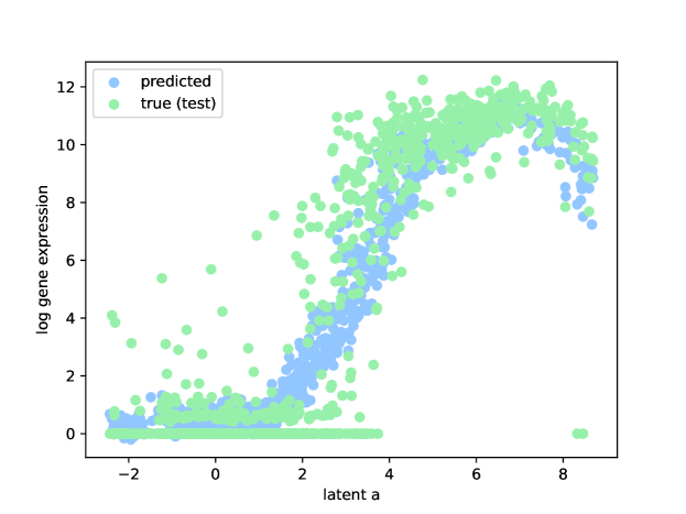
Figure 3: The figure shows predictions (blue) for unseen gene expression data given an embedding, generated with a graph GP, fit using the ProbDR-UMAP framework. The fit achieves a better predictive test RMSE than a VAE.

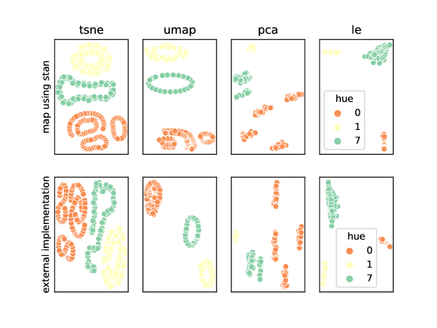
Figure 4: The figure shows embeddings of a few rotated MNIST figures recovered through automated MAP estimation using the PPL Stan with ProbDR assumptions, compared with popular community implementations.

4 Conclusion

We introduce the ProbDR framework that provides a unified perspective on a large number of DR algorithms. As an immediate consequence, PPLs can be used to perform DR via automated inference (e.g. Figure 4), and our framework allows these methods to be used with generative models (e.g. Figure 3; further detail is provided in Appendix C). We show that our framework is internally consistent (see Section B.6), and that marginalising the intermediary moment and discarding the variational constraint leads to GP behaviour in the generative models (Theorem B.21). Future work will aim to study the characteristics of constraints set by the various DR algorithms’ corresponding variational approximations. We will also explore whether these constraints can be used to guide kernel choice for defining GPs on manifolds (Borovitskiy et al., 2022), for instance hyperbolic kernels representing tree structures (Nickel and Kiela, 2017) and hyperspherical kernels representing cyclicality.

Appendix A Proof of (t-)SNE and UMAP results and remarks

A.1 Derivation of the main objective

We first show that a derivation of the ELBO from first principles in the ProbDR framework, and then show that the individual algorithms ((t-)SNE and UMAP) minimize the KL divergence found in our ELBO. The objective, an evidence lower bound, is derived as follows,

$$\text{KL}(q(\mathbf{M}|\mathbf{Y})||p_{\theta}(\mathbf{M}|\mathbf{X},\mathbf{Y})) =\mathbb{E}_{q(\mathbf{M}|\mathbf{Y})}\left[\dfrac{\log q(\mathbf{M}|\mathbf{Y})}{\log p_{\theta}(\mathbf{M}|\mathbf{X},\mathbf{Y})}\right]$$

$$=\mathbb{E}_{q(\mathbf{M}|\mathbf{Y})}[\log q(\mathbf{M}|\mathbf{Y})]-\mathbb{E}_{q(\mathbf{M}|\mathbf{Y})}[\log p_{\theta}(\mathbf{Y}|\mathbf{M})p(\mathbf{M}|\mathbf{X})]+\log p(\mathbf{Y})$$

$$=\mathbb{E}_{q(\mathbf{M}|\mathbf{Y})}\left[\dfrac{\log q(\mathbf{M}|\mathbf{Y})}{\log p(\mathbf{M}|\mathbf{X})}\right]-\mathbb{E}_{q(\mathbf{M}|\mathbf{Y})}[\log p_{\theta}(\mathbf{Y}|\mathbf{M})]+\log p(\mathbf{Y})$$

$$=\text{KL}(q(\mathbf{M}|\mathbf{Y})\|p(\mathbf{M}|\mathbf{X}))-\mathbb{E}_{q(\mathbf{M}|\mathbf{Y})}[\log p_{\theta}(\mathbf{Y}|\mathbf{M})]+\log p(\mathbf{Y})$$

$$=\log p(\mathbf{Y})-\text{ELBO}(\mathbf{X},\theta).$$

As $\log p(\mathbf{Y})$ is constant,

$$\operatorname*{arg\,min}_{\theta,\mathbf{X}}\text{KL}(q(\mathbf{M}|\mathbf{Y})||p_{\theta}(\mathbf{M}|\mathbf{X},\mathbf{Y}))=\operatorname*{arg\,max}_{\theta,\mathbf{X}}\text{ELBO}(\mathbf{X},\theta).$$

In the derivation above, we assume an improper uniform prior over $\mathbf{X}$, i.e. $p(\mathbf{X})\propto 1$. Our objective may also be interpreted as a regularised Bayesian inference (Zhu et al., 2014) objective.

Optimising the ELBO w.r.t. $\mathbf{X}$ leads to the minimisation problem becoming,

$$\operatorname*{arg\,max}_{\theta,\mathbf{X}}\text{ELBO}(\mathbf{X},\theta)=\operatorname*{arg\,min}_{\mathbf{X}}\text{KL}(q(\mathbf{M}|\mathbf{Y})||p(\mathbf{M}|\mathbf{X})),$$ (5)

as the data fit term of the ELBO (the first term in Equation 2) is independent of $\mathbf{X}$ and the KL above is independent of $\theta$. Below, we show how this KL divergence of Equation 5 arises in (t-)SNE and UMAP.

A.2 SNE

The stochastic neighbour embedding (SNE) algorithm was introduced by Hinton and Roweis (2002) as an approach for dimensionality reduction. The approach was to minimise a Kullback Leibler (KL) divergence between a set of probabilities $v^{S}_{ij}$ (corresponding to two data points $i$ and $j$ being neighbours) generated by a discrete distribution in a data space $\mathbf{Y}$ and a discrete distribution with probabilities $w_{ij}^{S}$ generated by using a lower dimensional latent embedding $\mathbf{X}$. These probabilities are defined as,

$$v_{ij}^{S} =\frac{\exp(-\|\mathbf{Y}_{i:}-\mathbf{Y}_{j:}\|^{2}/\sigma_{i}^{2})}{\sum_{k\neq i}\exp(-\|\mathbf{Y}_{i:}-\mathbf{Y}_{k:}\|^{2}/\sigma_{i}^{2})},$$

$$w_{ij}^{S} =\frac{\exp(-\|\mathbf{X}_{i:}-\mathbf{X}_{j:}\|^{2})}{\sum_{k\neq i}\exp(-\|\mathbf{X}_{i:}-\mathbf{X}_{k:}\|^{2})},$$

where $\mathbf{M}_{i:}$ and $\mathbf{M}_{:j}$ denote row $i$ and column $j$ of a matrix $\mathbf{M}$ respectively and $\sigma_{i}$ denotes a hyperparameter. Probabilities $w_{ij}^{S}$ are made close to probabilities $v_{ij}^{S}$ by minimizing the objective below with respect to $\mathbf{X}$,

$$\mathcal{C}_{SNE}=\sum_{i}\sum_{j\neq i}v_{ij}^{S}\log\frac{v_{ij}^{S}}{w_{ij}^{S}}.$$

The idea is that if probabilities defined in latent space are similar in terms of the KL divergence to probabilities defined in data space, then the latent dimensions of $\mathbf{X}$ are capturing some salient aspect of the data $\mathbf{Y}$. In all three algorithms, probabilities of association relating to the same point, $v_{ii}\text{ and }w_{ii}$, are set to zero.

Proof A.4.

of Theorem 2.1, SNE case. Now that we’ve introduced the SNE probabilities, we prove how it fits into the ProbDR framework.
In the case of SNE, we assume in the ProbDR framework,

$$q(\mathbf{A}^{\prime}|\mathbf{Y}) =\prod_{i}^{n}\text{Categorical}(\mathbf{A}^{\prime}_{i:};\mathbf{Y})=\prod_{i}^{n}\prod_{j\neq i}^{n}[v_{ij}^{S}]^{\mathbf{A}_{ij}}\text{ and}$$

$$p(\mathbf{A}^{\prime}|\mathbf{X}) =\prod_{i}^{n}\text{Categorical}(\mathbf{A}^{\prime}_{i:}|\mathbf{X})=\prod_{i}^{n}\prod_{j\neq i}^{n}[w_{ij}^{S}]^{\mathbf{A}_{ij}}.$$

This leads to the KL of Equation 5,

$$\text{KL}(q(\mathbf{A}^{\prime}|\mathbf{Y})||p(\mathbf{A}^{\prime}|\mathbf{X})) =\sum_{i}\text{KL}(q(\mathbf{A}^{\prime}_{i:})||p(\mathbf{A}^{\prime}_{i:}|\mathbf{X}))$$

$$=\sum_{i}\sum_{j\neq i}v_{ij}^{S}\log\frac{v_{ij}^{S}}{w_{ij}^{S}}=C_{SNE}.$$

A.3 Remark on the direction of KL and notation

Note that our notation (and only the notation) is flipped w.r.t. the (t-)SNE papers, i.e. we define the objective as $\text{KL}(q\|p)$ rather than $\text{KL}(p\|q)$, although the computation of the objective remains the same.

To see why, note that the objective of Hinton and Roweis (2002) looks like,

$$\text{KL}(\text{probabilities involving data}\|\text{probabilities involving latents}).$$

Noting that in typical variational models (such as VAEs and variational GPLVMs), the variational distributions are a function of data, and the model distributions are a function of latents (or parameters associated with the generative model), we propose that it is more natural to set the data based probabilities to $q$ and write the objective as $\text{KL}(q\|p)$ as we do here. Noting this was one of the main inspirations for this project, along with the observation that many circularly-specified modelling methodologies can be written as variational inference algorithms. Note further that we denote high dimensional observed data by $\mathbf{Y}$ and low dimensional embeddings by $\mathbf{X}$, taking inspiration from how regression models are typically specified, whereas many older works such as (t-)SNE use reversed notation.

A.4 t-SNE

The t-SNE algorithm was introduced by van der Maaten and Hinton (2008) to improve optimisation and visualization. In the t-SNE algorithm, probabilities $v_{ij}^{t}$ and $w_{ij}^{t}$ are defined as,

$$v_{ij}^{t} =(v_{ij}^{S}+v_{ji}^{S})/2n,$$

$$w_{ij}^{t} =\frac{(1+\|\mathbf{X}_{i:}-\mathbf{X}_{j:}\|^{2})^{-1}}{\sum_{k\neq l}(1+\|\mathbf{X}_{k:}-\mathbf{X}_{l:}\|^{2})^{-1}},$$

which are then matched by minimizing the cost function below w.r.t $\mathbf{X}$,

$$\mathcal{C}_{t-SNE}=\sum_{i\neq j}v_{ij}^{t}\log\frac{v_{ij}^{t}}{w_{ij}^{t}}.$$

Note that the normalization here, as opposed to SNE, is over the entire set of probabilities.

Proof A.5.

of Theorem 2.1, t-SNE case. Now that we’ve introduced the t-SNE probabilities, we prove how it fits into the ProbDR framework. Note that both sets of probabilities in t-SNE sum up to one. In the case of t-SNE, we assume in the ProbDR framework,

$$q(\mathbf{A}^{\prime}|\mathbf{Y}) =\text{Categorical}(\text{vec}(\mathbf{A}^{\prime})|\mathbf{Y})=\prod_{i\neq j}^{n}[v_{ij}^{t}]^{\mathbf{A}_{ij}}\text{ and}$$

$$p(\mathbf{A}^{\prime}|\mathbf{X}) =\text{Categorical}(\text{vec}(\mathbf{A}^{\prime})|\mathbf{X})=\prod_{i\neq j}^{n}[w_{ij}^{t}]^{\mathbf{A}_{ij}}.$$

Therefore the KL of Equation 5,

$$\text{KL}(q(\mathbf{A}^{\prime}|\mathbf{Y})||p(\mathbf{A}^{\prime}|\mathbf{X})) =\sum_{i\neq j}v_{ij}^{t}\log\frac{v_{ij}^{t}}{w_{ij}^{t}}=C_{t-SNE}.$$

A.5 UMAP

The UMAP algorithm (McInnes et al., 2020) has proven to be a popular choice in computational biology for visualizing single-cell RNA-seq data due to decreased runtimes and a greater ability of recovering cell clusters as compared with t-SNE (Becht et al., 2019). The algorithm defines probabilities $v_{ij}^{U}$ and $w_{ij}^{U}$ as

$$v_{i|j}^{U} =\exp((\rho_{i}-\text{distance}(\mathbf{Y}_{i:},\mathbf{Y}_{j:}))/\sigma_{i}),$$

$$v_{ij}^{U} =v_{i|j}+v_{j|i}-v_{i|j}*v_{j|i},$$

$$w_{ij}^{U} =(1+a\|\mathbf{X}_{i:}-\mathbf{X}_{j:}\|^{2b})^{-1},$$

where $\rho_{i}$ denotes the distance to the nearest neighbour of data point $i$. These are matched by optimizing the cost function below w.r.t $\mathbf{X}$:

$$\mathcal{C}_{UMAP}=\sum_{i\neq j}v_{ij}^{U}\log\frac{v_{ij}^{U}}{w_{ij}^{U}}+(1-v_{ij}^{U})\log\frac{1-v_{ij}^{U}}{1-w_{ij}^{U}}.$$

Proof A.6.

of Theorem 2.1, UMAP case. Now that we’ve introduced the UMAP probabilities, we prove how it fits into the ProbDR framework. We use UMAP notation for defining probabilities (i.e. $v$ and $w$) throughout this paper.
In the case of UMAP, we assume in the ProbDR framework,

$$q(\mathbf{A}^{\prime}|\mathbf{Y}) =\prod_{i<j}^{n}\text{Bernoulli}(\mathbf{A}^{\prime}_{ij};\mathbf{Y})=\prod_{i}^{n}\prod_{j<i}^{n}[v_{ij}^{U}]^{\mathbf{A}^{\prime}_{ij}}[1-v_{ij}^{U}]^{1-\mathbf{A}^{\prime}_{ij}}\text{ and}$$

$$p(\mathbf{A}^{\prime}|\mathbf{X}) =\prod_{i<j}^{n}\text{Bernoulli}(\mathbf{A}^{\prime}_{ij}|\mathbf{X})=\prod_{i}^{n}\prod_{j<i}^{n}[w_{ij}^{U}]^{\mathbf{A}^{\prime}_{ij}}[1-w_{ij}^{U}]^{1-\mathbf{A}^{\prime}_{ij}}.$$

Hence,

$$\text{KL}(q(\mathbf{A}^{\prime}|\mathbf{Y})||p(\mathbf{A}^{\prime}|\mathbf{X})) =\sum_{i}\sum_{j<i}\text{KL}(q(\mathbf{A}^{\prime}_{ij})||p(\mathbf{A}^{\prime}_{ij}|\mathbf{X}))$$

$$=\sum_{i}\sum_{j<i}v_{ij}^{U}\log\frac{v_{ij}^{U}}{w_{ij}^{U}}+(1-v_{ij}^{U})\log\frac{1-v_{ij}^{U}}{1-w_{ij}^{U}}=C_{UMAP}/2.$$

A.6 Remarks on adjacencies, Laplacians and marginal variances

A note on adjacency matrices: In models corresponding to SNE and t-SNE, the adjacency matrix we define ($\mathbf{A}^{\prime}$) can be thought of as an adjacency matrix on a directed graph; the use of categorical distributions results in $\mathbf{A}^{\prime}$ being asymmetric. In the UMAP case, the matrix $\mathbf{A}^{\prime}$ also represents a directed graph as the lower triangle of the adjacency matrix is independent of the upper triangle (hence, samples of the matrix are likely to be asymmetric). However, by changing the range of the sum of the UMAP cost function to $i<j$ rather than summing over $i\neq j$ (which simply results in a factor of a half appearing before the cost function), one may construct a lower triangular adjacency matrix, describing a directed acyclical graph, which may be made symmetric as needed (as in Section 2). Adjacency matrices representing DAGs or more generally directed graphs can be used as part of other generative models described in Appendix E.

A note on marginal variances: A covariance $\mathbf{C}$ can be normalized as,

$$\text{diag}(\mathbf{C})^{-1/2}\mathbf{C}\text{diag}(\mathbf{C})^{-1/2},$$

to make it a correlation matrix with uniform marginal variances. This process can be done approximately, efficiently and differentiably by using the eigendecomposition of the covariance or the precision.

A note on the Laplacian as a precision: The Laplacian as part of a precision matrix is meaningful as it is positive definite, describes non-negative partial correlations between data points (and where the partial correlation is zero, data points are conditionally independent), and is typically sparse, describing a sparsely-connected Gaussian field on the data.

Appendix B Two-Step MLE Proofs & Wishart Results

B.1 Remark on notation used for Wishart matrices

Many of our statements involving Wishart distributed random matrices are denoted as,

$$\mathbf{T}\sim\mathcal{W}(\hat{\mathbf{M}},d).$$

The random matrix without a hat or an overset tilda $\mathbf{T}$ represents a matrix that is scaled in some way, and matrices with a hat or overset tilda represent unscaled quantities. In this example, note that $\mathbb{E}(\mathbf{T})=\hat{\mathbf{M}}*d$. Therefore, sample (estimated) covariances in our work are denoted as $\hat{\mathbf{S}}$, as they are typically calculated as $\mathbf{Y}\mathbf{Y}^{T}/d$, and hence are an unscaled quantity. In this example, we would denote by $\mathbf{S}$ the unscaled random matrix $\mathbf{Y}\mathbf{Y}^{T}$, which (assuming that the columns of $\mathbf{Y}$ are independent multivariate normal samples) by definition is Wishart distributed, and is scaled by the degrees of freedom in expectation.

B.2 Summary of main result

The main result stated in Theorem 3.2 states that the MAP estimation for $\mathbf{X}$ given the models (with an improper uniform prior over $\mathbf{X}$) occurs at the $l$ major and minor scaled eigenvectors respectively,

$$\hat{\mathbf{\mathbf{S}}}*d|\mathbf{X}\sim\mathcal{W}\left(\mathbf{X}\mathbf{X}^{T}+\sigma^{2}\mathbf{I}_{n},d\right)\quad \Rightarrow\quad\hat{\mathbf{X}}_{\text{MAP}}=\mathbf{U}_{l\text{ maj}}(\mathbf{\Lambda}_{l\text{ maj}}-\hat{\sigma}^{2}\mathbf{I}_{l})^{1/2}\mathbf{R}^{T}$$

$$\hat{\mathbf{\Gamma}}*d|\mathbf{X}\sim\mathcal{W}\left((\mathbf{X}\mathbf{X}^{T}+\beta\mathbf{I}_{n})^{-1},d\right)\quad \Rightarrow\quad\hat{\mathbf{X}}_{\text{MAP}}=\mathbf{U}_{l\text{ min}}(\mathbf{\Lambda}^{-1}_{l\text{ min}}-\hat{\beta}\mathbf{I}_{l})^{1/2}\mathbf{R}^{T}$$

where $\mathbf{U}_{l}$ is a matrix of $l-$eigenvectors, $\mathbf{\Lambda}_{l}$ is a diagonal matrix of $l$ corresponding eigenvalues and $\mathbf{R}$ is an arbitrary rotation matrix. $l$ maj and min denote the eigencomponents corresponding to the $l$-largest and lowest eigenvalues respectively.

Note that, in this work for simplicity, we generally assume that $\mathbf{Y}$ has a zero mean and doesn’t need to be centered and that generative models for $\mathbf{Y}$ may be set to have a zero mean.

This is due to two key results, probabilistic principal coordinate analysis (of Lawrence (2005), based on Tipping and Bishop (1999)) and probabilistic minor coordinate analysis (which we derive, based on results of Williams and Agakov (2002)).

B.3 Probabilistic principal coordinate analysis based results

First note that, for some applications, multivariate normal likelihoods and Wishart likelihoods are equal, up to additive constants.

Lemma B.7.

Let $\mathbf{F}\in\mathbb{R}^{n\times d}$ and $\mathbf{T}\equiv\tilde{\mathbf{T}}*d\equiv\mathbf{F}\mathbf{F}^{T}$. The log likelihood of the following models is equal up to additive constants that do not depend on $\mathbf{M}$,

$$\log p(\mathbf{F}|\mathbf{M})\text{ assuming }\mathbf{F}|\mathbf{M} \sim\mathcal{MN}(0,\mathbf{M},\mathbf{I}_{d})\text{ and },$$

$$\log p(\mathbf{T}|\mathbf{M})\text{ assuming }\mathbf{T}|\mathbf{M} \sim\mathcal{W}\left(\mathbf{M},d\right).$$

Proof B.8.

of Lemma B.7.

In the normal case,

$$\mathcal{L}(\mathbf{F})=\log p(\mathbf{F}|\mathbf{M}) =-\dfrac{1}{2}\text{tr}\left(\mathbf{I}_{d}\mathbf{F}^{T}\mathbf{M}^{-1}\mathbf{F}\right)-\dfrac{d}{2}\log|\mathbf{M}|-\dfrac{n}{2}\log|\mathbf{I}_{d}|-\dfrac{np}{2}\log 2\pi$$

$$=-\dfrac{{\color[rgb]{1,0,0}d}}{2}\text{tr}\left({\color[rgb]{1,0,0}\dfrac{1}{d}}\mathbf{F}\mathbf{F}^{T}\mathbf{M}^{-1}\right)-\dfrac{d}{2}\log|\mathbf{M}|+c,\text{\hskip 42.67912pt (trace is cyclic)}$$

$$=-\dfrac{d}{2}\text{tr}\left(\tilde{\mathbf{T}}\mathbf{M}^{-1}\right)-\dfrac{d}{2}\log|\mathbf{M}|+c.$$

In the Wishart case when $d\geq n$, the sampling distribution of $\mathbf{F}\mathbf{F}^{T}$ is by definition Wishart, so the likelihood w.r.t. $\tilde{\mathbf{S}}$ can be obtained easily,

$$\mathcal{L}(\mathbf{F})=\log p_{\mathcal{W}}(\tilde{\mathbf{T}}*d|\mathbf{M})=-\dfrac{d}{2}\text{tr}\left(\mathbf{M}^{-1}\tilde{\mathbf{T}}\right)-\dfrac{d}{2}\log|\mathbf{M}|+c.$$

In the case when $d<n$, the distribution of $\mathbf{F}\mathbf{F}^{T}$ is a singular Wishart (Uhlig, 1994). The likelihood can be computed using Theorem 6 of Uhlig (1994), and is identical to the statement above up to additive constants.

$$\mathcal{L}(\mathbf{F})=\log p_{\mathcal{W}}(\tilde{\mathbf{T}}*d|\mathbf{M})=-\dfrac{d}{2}\text{tr}\left(\mathbf{M}^{-1}\tilde{\mathbf{T}}\right)-\dfrac{d}{2}\log|\mathbf{M}|+c.$$

Lemma B.9 (Probabilistic Principal Coordinates Analysis (PCA)).

The maximum likelihood estimate of $\mathbf{X}$ assuming the model,

$$\mathcal{N}(\mathbf{Y}|0,\mathbf{X}\mathbf{X}^{T}+\sigma^{2}I)\text{ or }\mathcal{W}(\mathbf{S}|\mathbf{X}\mathbf{X}^{T}+\sigma^{2}I,d)$$

where $\mathbf{S}\equiv\tilde{\mathbf{S}}*d=\mathbf{Y}\mathbf{Y}^{T}$ and the corresponding optimisation is,

$$\operatorname*{arg\,max}_{\mathbf{X}}\hskip 5.69046pt-\frac{d}{2}\log|\mathbf{C}|-\frac{d}{2}\text{tr}(\tilde{\mathbf{S}}\mathbf{C}^{-1})+c,$$

occurs at,

$$\hat{\mathbf{X}}=\mathbf{U}_{l}(\mathbf{\Lambda}_{l}-\hat{\sigma}^{2}\mathbf{I}_{l})^{1/2}\mathbf{R}^{T},$$

where $\hat{\sigma}^{2}=\frac{\sum_{i=l+1}^{n}\lambda_{i}}{n-l}$ and $\mathbf{U}_{l}\text{ and }\mathbf{\Lambda}_{l}$ are the matrices of $l$ major eigenvectors and eigenvalues of $\tilde{\mathbf{S}}$.

Proof B.10.

of Lemma B.9.

The Wishart model is equivalent to the normal case due to Lemma B.7. The main result is due to Lawrence (2005), which is based on Tipping and Bishop (1999).

This proves the first claim of Theorem 3.2.

Remark on equivalent inverse wishart statements: Wishart distributions and inverse-Wishart distributions are closely tied,

$$\mathbf{W}\sim\mathcal{W}(\mathbf{M},\rho)\Leftrightarrow\mathbf{W}^{-1}\sim\mathcal{W}^{-1}(\mathbf{M}^{-1},\rho),$$

and so many of the Wishart sampling statements can also be written instead with inverse-Wisharts.

B.4 Probabilistic minor coordinate analysis based results

In this section, we will prove the second Wishart statement of Theorem 3.2. We do so by first describing a novel probabilistic dimensionality reduction model, probabilistic minor coordinates analysis.

Theorem B.11 (Minor Coordinates Analysis (MCA)).

We propose a dimensionality reduction method utilising the result of probabilistic minor components analysis (Williams and Agakov, 2002). Using this algorithm, and given an estimated/empirical precision matrix $\tilde{\mathbf{\Gamma}}$, we find a low dimensional embedding $\mathbf{X}$ by maximising objectives of the form below.

Let $\mathbf{X}\in\mathbb{R}^{n\times l}$ and $\mathbf{\Gamma}\equiv\tilde{\mathbf{\Gamma}}*d$. Then,

$$\operatorname*{arg\,max}_{\mathbf{X}}\hskip 5.69046pt\frac{d}{2}\log|\mathbf{P}^{-1}|-\frac{d}{2}\text{tr}(\mathbf{P}^{-1}\tilde{\mathbf{\Gamma}})+c$$

with $\mathbf{P}^{-1}\equiv\mathbf{X}\mathbf{X}^{T}+\beta\mathbf{I}_{n}$ is attained at,

$$\hat{\mathbf{X}}=\mathbf{U}_{l}(\mathbf{\Lambda}^{-1}_{l}-\hat{\beta}\mathbf{I}_{l})^{1/2}\mathbf{R}^{T},$$

where $\hat{\beta}=\frac{n-l}{\sum_{i=l+1}^{n}\lambda_{i}}$ and $\mathbf{U}_{l}\text{ and }\mathbf{\Lambda}_{l}$ are the matrices of $l$ minor eigenvectors and eigenvalues of $\tilde{\mathbf{\Gamma}}$.

Proof B.12.

of Theorem B.11

The result is based on the result of Williams and Agakov (2002) if one starts with the notation $\tilde{\mathbf{\Gamma}}$, $\mathbf{P}^{-1}$, $\mathbf{X}$, $n$, $d$, $l$ instead of $\mathbf{S}$, $\mathbf{C}^{-1}$, $\mathbf{W}$, $d$, $N$, $m$.

More explicitly, it’s been shown in Williams and Agakov (2002), that the maximum likelihood estimate of the parameter ${\color[rgb]{0,0,1}\mathbf{W}}\in\mathbb{R}^{{\color[rgb]{0,0,1}d}\times{\color[rgb]{0,0,1}m}}$, in objectives of the form below,

$$\mathcal{L}=\frac{{\color[rgb]{0,0,1}N}}{2}\log|{\color[rgb]{0,0,1}\mathbf{C}}^{-1}|-\frac{{\color[rgb]{0,0,1}N}}{2}\text{tr}({\color[rgb]{0,0,1}\mathbf{C}}^{-1}{\color[rgb]{0,0,1}\mathbf{S}})+c,$$

with ${\color[rgb]{0,0,1}\mathbf{C}}^{-1}\equiv{\color[rgb]{0,0,1}\mathbf{W}\mathbf{W}^{T}}+\beta\mathbf{I}_{{\color[rgb]{0,0,1}d}}$, is,

$$\hat{{\color[rgb]{0,0,1}\mathbf{W}}}=\mathbf{U}_{{\color[rgb]{0,0,1}m}}(\mathbf{\Lambda}^{-1}_{{\color[rgb]{0,0,1}m}}-\hat{\beta}\mathbf{I}_{{\color[rgb]{0,0,1}m}})^{1/2}\mathbf{R}^{T},$$

where $\hat{\beta}=\frac{{\color[rgb]{0,0,1}d}-{\color[rgb]{0,0,1}m}}{\sum_{i={\color[rgb]{0,0,1}m}+1}^{{\color[rgb]{0,0,1}d}}\lambda_{i}}$ and $\mathbf{U}_{{\color[rgb]{0,0,1}m}}\text{ and }\mathbf{\Lambda}_{{\color[rgb]{0,0,1}m}}$ are the matrices of ${\color[rgb]{0,0,1}m}$ minor eigenvectors and eigenvalues of ${\color[rgb]{0,0,1}\mathbf{S}}$. Key notation has been highlighted in blue. If notation is changed as follows, ${\color[rgb]{0,0,1}\mathbf{S}}\rightarrow\tilde{\mathbf{\Gamma}}$, ${\color[rgb]{0,0,1}\mathbf{C}^{-1}}\rightarrow\mathbf{P}^{-1},{\color[rgb]{0,0,1}\mathbf{W}}\rightarrow\mathbf{X}$, ${\color[rgb]{0,0,1}d}\rightarrow n$, ${\color[rgb]{0,0,1}N}\rightarrow d$, ${\color[rgb]{0,0,1}m}\rightarrow l$, the proposed statement follows.

The probabilistic interpretation of this is trivial and is laid out below.

Lemma B.13 (Probabilistic Minor Coordinates Analysis).

Minor coordinates analysis is maximum likelihood inference given the model,

$$\mathbf{\Gamma}|\mathbf{X}\sim\mathcal{W}\left((\mathbf{X}\mathbf{X}^{T}+\beta\mathbf{I}_{n})^{-1},d\right)$$

where $\tilde{\mathbf{\Gamma}}\equiv\mathbf{\Gamma}/d$ is an empirical precision matrix, for example, calculated as $(\mathbf{Y}\mathbf{Y}^{T}/d)^{-1}$.

Proof B.14.

of Lemma B.13.

The objective in Theorem B.11 is the likelihood of the models in Lemma B.7 with $\tilde{\mathbf{T}}=\tilde{\mathbf{\Gamma}}$.

Probabilistic minor coordinates analysis is the second statement of Theorem 3.2, hence completing the proof of our main statement.

B.5 ProbDR & 2-step MAP equivalence

Now, we show that the two step MAP inference process is equivalent to ProbDR.

Theorem B.15 (ProbDR KL minimisation and MAP Equivalence: Wishart Case).

The Maximum a posteriori estimate for $\mathbf{X}$, i.e. $\operatorname*{arg\,max}_{\mathbf{X}}\log p(\hat{\mathbf{M}}(\mathbf{Y})*d|\mathbf{X})$ assuming

$$p(\mathbf{M}|g(\mathbf{X}))=\mathcal{W}(\mathbf{M}|g(\mathbf{X}),d)$$

and an improper uniform prior is equivalent to finding $\operatorname*{arg\,min}_{\mathbf{X}}\text{KL}(q(\mathbf{M}|\hat{\mathbf{M}}(\mathbf{Y}))\|p(\mathbf{M}|g(\mathbf{X}))))$ in the variational setup,

$$\text{model (law of p)}:\mathbf{M}|g(\mathbf{X}) \sim\mathcal{W}(g(\mathbf{X}),d),$$

$$\text{variational approx (law of q)}:\mathbf{M}|\hat{\mathbf{M}}(\mathbf{Y}) \sim\mathcal{W}(\hat{\mathbf{M}}(\mathbf{Y}),d).$$

Proof B.16.

of Theorem B.15.

In the maximum likelihood setup, the negative log likelihood is as follows,

$$-\log p(\hat{\mathbf{M}}(\mathbf{Y})*d|\mathbf{X})=\dfrac{d}{2}\text{tr}(g(\mathbf{X})^{-1}\hat{\mathbf{M}}(\mathbf{Y}))+\frac{d}{2}\log|g(\mathbf{X})|.$$

Using the result of KL divergence between two Wishart distributions, the variational bound can be written as,

$$\text{KL}(q(\mathbf{M}|\hat{\mathbf{M}}(\mathbf{Y}))\|p(\mathbf{M}|\mathbf{X})))=\frac{d}{2}\left(\log|g(\mathbf{X})|-k\right)+\dfrac{d}{2}\text{tr}(g(\mathbf{X})^{-1}\hat{\mathbf{M}}(\mathbf{Y}))+c.$$

The bounds are equal up to additive constants.

Such a result is true for many exponential family (see Jordan (2009) for a definition) distributions, as for exponential family densities $p$ and $q$, where $q$ has no parameters of interest,

$$-\text{KL}(q\|p) =-\mathbb{E}_{q}(\log q(\mathbf{x})/\log p(\mathbf{x}))$$

$$=-[\eta(\theta_{q})-\eta(\theta_{p})]^{T}\cdot\mathbb{E}_{q}(\mathbf{T(x)})+[A(\eta_{q})-A(\eta_{p})]$$

$$=\eta(\theta_{p})^{T}\cdot\mathbb{E}_{q}(\mathbf{T(x)})-A(\eta_{p})+c,$$

which is the log likelihood of the exponential family distribution $p$, up to a constant, with the expectation of the sufficient statistic under the variational distribution being set to the observed sufficient statistic.

Next, we show some consistency results.

B.6 Consistency of PCA & MCA, and ProbDR marginal consistency proofs

Firstly, we show that pPCA and pMCA obtain the same solution, even though they are not equivalent statements.

Lemma B.17 (Equivalence of probabilistic PCA and probabilistic MCA).

Let $\tilde{\mathbf{S}}\equiv\mathbf{S}/d\equiv\mathbf{Y}\mathbf{Y}^{T}/d$ and $\tilde{\mathbf{\Gamma}}\equiv\mathbf{\Gamma}/d\equiv\tilde{\mathbf{S}}^{-1}$. The matrices $\tilde{\mathbf{S}}\text{ and }\tilde{\mathbf{\Gamma}}$ share eigenvectors, represented by the matrix $\mathbf{U}$ and their diagonal eigenvalue matrices are $\mathbf{\Lambda}_{\tilde{\mathbf{S}}}$ and $\mathbf{\Lambda}_{\tilde{\mathbf{S}}}^{-1}$ respectively. Then, the estimated covariance assuming either of the following models,

$$\mathbf{S}|\mathbf{X} \sim\mathcal{W}\left(\mathbf{X}\mathbf{X}^{T}+\sigma^{2}\mathbf{I},d\right)$$

$$\mathbf{\Gamma}|\mathbf{X} \sim\mathcal{W}\left((\mathbf{X}\mathbf{X}^{T}+\beta\mathbf{I})^{-1},d\right)$$

is identical.

Proof B.18.

of Lemma B.17.
The proof is due to Lemma B.9 and Lemma B.13. In PCA,

$$\hat{\mathbf{S}}_{\text{PCA}}=\hat{\mathbf{X}}\hat{\mathbf{X}}^{T}+\hat{\sigma}^{2}\mathbf{I}=\mathbf{U}\mathbf{\Lambda}_{\hat{\mathbf{S}}}\mathbf{U}^{T},$$

and in MCA,

$$\hat{\mathbf{S}}_{\text{MCA}}=\hat{\mathbf{X}}\hat{\mathbf{X}}^{T}+\hat{\beta}\mathbf{I}=\mathbf{U}\mathbf{\Lambda}^{-1}_{\hat{\mathbf{\Gamma}}}\mathbf{U}^{T}=\mathbf{U}\mathbf{\Lambda}_{\hat{\mathbf{S}}}\mathbf{U}^{T}=\hat{\mathbf{S}}_{\text{PCA}}.$$

Note that, although the covariance estimates are the same, the noise levels are not.

Theorem B.19 (Estimated noise level in PCA and MCA).

The estimated noise level in MCA $\hat{\beta}$ is lower than its counterpart in PCA $\hat{\sigma}^{2}$,

$$\hat{\beta}\leq\hat{\sigma}^{2}.$$

Proof B.20.

of Theorem B.19.
Assume the setup of Lemma B.17 and let $\lambda$s be major eigenvalues of the sample covariance matrix.

Due to Lemma B.9, Theorem B.11, and due to the fact that the major eigenvalues of the sample covariance are minor eigenvalues of the precision,

$$\hat{\sigma}^{2}=\frac{\sum_{i=l+1}^{n}\lambda_{i}}{n-l}\text{ and }\hat{\beta}=\frac{n-l}{\sum_{i=l+1}^{n}\dfrac{1}{\lambda_{i}}}.$$

Therefore,

$$\dfrac{\hat{\sigma}^{2}}{\hat{\beta}} =\dfrac{\sum_{i=l+1}^{n}1/\lambda_{i}\sum_{i=l+1}^{n}\lambda_{i}}{(n-l)^{2}}\overset{\text{AM-GM}}{\geq}\sqrt[n-l]{\prod_{i}\lambda_{i}/\lambda_{i}}=1.$$

Below, we show that marginalising the moment in either case of our Wishart models leads to the standard Gaussian process assumed in many linear DR models (i.e. one with a dot product kernel). We do not show how column independence arises, although this is trivial plugging in $\text{vec}(\mathbf{Y})$ into the results below and using the matrix normal distribution’s definitions.

Theorem B.21 (Marginal consistency with PCA).

Assuming a PCA-esque generative model,

$$\mathbf{y}|\mathbf{S} \sim\mathcal{N}\left(\mathbf{0},\dfrac{1}{\rho}\mathbf{S}\right),$$

$$\mathbf{S}|\mathbf{X} \sim\mathcal{W}(\mathbf{X}\mathbf{X}^{T}+\sigma^{2}\mathbf{I},\rho),$$

or a MCA-esque generative model,

$$\mathbf{y}|\mathbf{S} \sim\mathcal{N}\left(\mathbf{0},\mathbf{S}*(\rho-n+1)\right),$$

$$\mathbf{S}|\mathbf{X} \sim\mathcal{W}^{-1}\left(\mathbf{X}\mathbf{X}^{T}+\beta\mathbf{I},\rho\right)$$

the marginal distribution of any column of the data $\mathbf{y}$, as $\rho\rightarrow\infty$, is given by,

$$\mathbf{y}|\mathbf{X}\sim\mathcal{N}(\mathbf{0},\mathbf{X}\mathbf{X}^{T}+\sigma^{2}\mathbf{I}).$$

Proof B.22.

of Theorem B.21.

In the first case,

$$\text{Var}\left(\dfrac{\mathbf{S}_{ij}}{\rho}\right)=\dfrac{\left([\mathbf{X}\mathbf{X}^{T}]_{ij}^{2}+[\sigma^{2}+\mathbf{X}\mathbf{X}^{T}]_{ii}[\sigma^{2}+\mathbf{X}\mathbf{X}^{T}]_{jj}\right)_{ij}\rho}{\rho^{2}}\rightarrow 0\text{ and,}$$

$$\mathbb{E}\left(\dfrac{\mathbf{S}}{\rho}\right)=\mathbf{X}\mathbf{X}^{T}+\sigma^{2}\mathbf{I}.$$

Therefore, $\mathbf{S}/\rho$ converges to a constant matrix, hence the marginal in the limit is $\mathcal{N}(\mathbf{0},\mathbf{X}\mathbf{X}^{T}+\sigma^{2}\mathbf{I})$. In the second case, due to conjugacy (Murphy, 2023),

$$\mathbf{y}|\mathbf{X}\sim t_{\rho-n+1}(\mathbf{0},\mathbf{X}\mathbf{X}^{T}+\sigma^{2}\mathbf{I}),$$

which tends to the normal statement above as $\rho\rightarrow\infty$.

A note on Wishart-Normal conjugacy: Some common references state normal conjugacy results using atypical notation for Wishart distributions, so we prove the result above, using notation used in this paper, from first principles. Let $\mathbf{y}\sim\mathcal{N}(\mathbf{0},\kappa\mathbf{S})$ and $\mathbf{S}\sim\mathcal{W}^{-1}(\mathbf{M},d)$. Then,

$$p(\mathbf{y}) =\int p(\mathbf{y}|\mathbf{S})p(\mathbf{S})d\mathbf{S}$$

$$\propto|\mathbf{M}|^{d/2}\int|\mathbf{S}|^{-(d+n+2)/2}\exp(-\kappa^{-1}\mathbf{y}^{T}\mathbf{S}^{-1}\mathbf{y}/2-\text{tr}(\mathbf{M}\mathbf{S}^{-1}))d\mathbf{S}$$

$$\propto|\mathbf{M}|^{d/2}\int|\mathbf{S}|^{-(d+n+2)/2}\exp(-\text{tr}(\kappa^{-1}\mathbf{y}\mathbf{y}^{T}\mathbf{S}^{-1})/2-\text{tr}(\mathbf{M}\mathbf{S}^{-1}))d\mathbf{S}$$

$$\propto|\mathbf{M}|^{d/2}\int|\mathbf{S}|^{-(d+n+2)/2}\exp\left[-\text{tr}\Big{(}(\kappa^{-1}\mathbf{y}\mathbf{y}^{T}+\mathbf{M})\mathbf{S}^{-1})\Big{)}\right]d\mathbf{S}$$

$$\overset{\int p=1}{\propto}|\mathbf{M}|^{d/2}|\kappa^{-1}\mathbf{y}\mathbf{y}^{T}+\mathbf{M}|^{-(d+1)/2}$$

$$\propto|\mathbf{M}|^{d/2}|\mathbf{y}\mathbf{y}^{T}+\kappa\mathbf{M}|^{-(d+1)/2}$$

$$\propto|\mathbf{M}|^{-1/2}\left[1+\frac{1}{\kappa}\mathbf{y}^{T}\mathbf{M}^{-1}\mathbf{y}\right]^{-(d+1)/2}\qquad\text{ (matrix determinant lemma)}$$

$$\propto t_{d-n+1}\left(\mathbf{y}|\mathbf{0},\frac{\kappa\mathbf{M}}{d-n+1}\right).$$

B.7 Utility results (for PPLs and distributions of normal distances)

PPLs generally do not have support for degenerate Wishart distributions. Therefore, we use the trick below to deal with low-$d$, high-$n$ problems.

Lemma B.23.

Let $\mathbf{F}\in\mathbb{R}^{n\times d}$ and $\tilde{\mathbf{T}}\equiv\mathbf{F}\mathbf{F}^{T}/d$ with $d<n\leq\rho$. The following computation results in the log-likelihood of Lemma B.7 up to additive and multiplicative constants,

$$\log\mathcal{W}\left(\rho\tilde{\mathbf{T}}|\mathbf{M},\rho\right).$$

This is useful for usage with PPLs, when doing MAP inference, with no support for singular Wishart distributions - note that due to the multiplicative constant, models specified in the PPL must not contain any other sampling statements, or if they are present, the corresponding likelihoods must be appropriately weighted. Unlike in the case presented here, multiplicative constants do matter however, when doing MCMC sampling.

Proof B.24.

of Lemma B.23.

$$\mathcal{L}(\tilde{\mathbf{T}})=-\dfrac{\rho}{2}\text{tr}\left(\mathbf{M}^{-1}\tilde{\mathbf{T}}\right)-\dfrac{\rho}{2}\log|\mathbf{M}|+c,$$

which is equal to the likelihood of Lemma B.7 up to a factor of $d/\rho$ and an additive constant.

Below, we show that the Categorical/Bernoulli (i.e. (t-)SNE and UMAP) cases of the ProbDR framework are approximately equivalent to two step MAP. This is useful, for example, if one attempts to use a PPL for DR with limited support for variational inference.

Lemma B.25 ((t)-SNE/UMAP ProbDR is approximately two-step MAP).

Proof B.26.

of Lemma B.25. As our variational distributions do not have any optimised parameters,

$$\text{KL}_{\text{categorical}}(q\|p) =\sum_{i}q_{i}\log\left(\dfrac{q_{i}}{p_{i}}\right)$$

$$=-\sum_{i}q_{i}\log p_{i}+c$$

$$\approx-\dfrac{1}{n}\sum_{i}\lfloor nq_{i}\rfloor\log p_{i}+c.$$

So, the KL divergence of ProbDR in the (t-)SNE cases (i.e. with a categorical distribution on the probabilities of adjacency) is approximately equal to the negative log likelihood (up to an additive and multiplicative constant) of a categorical distribution with the observed random variables set to $\lfloor nq_{i}\rfloor$ for category (data point) $i$. The case for the Bernoulli follows as it is a special case of the categorical distribution.

Finally, for future work (for example, if graphs in the ProbDR-UMAP case are to be analysed as mixtures of graphs / hypergraphs arising due to kernel choice in a GP on a manifold), we note a simple result below that can be used to calculate adjacency probabilities.

Lemma B.27 (Distribution of normal distances).

$$\begin{bmatrix}\mathbf{y}_{i}\\ \mathbf{y}_{j}\end{bmatrix}\sim\mathcal{MN}\left(\mu,\begin{bmatrix}k_{ii}&k_{ij}\\ k_{ji}&k_{jj}\end{bmatrix},\mathbf{I}_{d}\right)$$

$$\Rightarrow\|\mathbf{y}_{i}-\mathbf{y}_{j}\|^{2}\sim\Gamma\left(\dfrac{d}{2},2(k_{ii}+k_{jj}-2k_{ij})\right).$$

Proof B.28.

of Lemma B.27.

$$\forall k:y_{i}^{k}-y_{j}^{k} \sim\mathcal{N}(0,k_{ii}+k_{jj}-2k_{ij})\overset{d}{=}\sqrt{k_{ii}+k_{jj}-2k_{ij}}Z$$

$$\Rightarrow\|\mathbf{y}_{i}-\mathbf{y}_{j}\|^{2}=\sum_{k}^{d}(y^{k}_{i}-y^{k}_{j})^{2} \overset{d}{=}(k_{ii}+k_{jj}-2k_{ij})\sum_{k}^{d}Z_{k}^{2}$$

$$\overset{d}{=}(k_{ii}+k_{jj}-2k_{ij})\chi^{2}_{d}$$

$$\overset{d}{=}\Gamma(k=d/2,\theta=2(k_{ii}+k_{jj}-2k_{ij})).$$

B.8 Equivalence of GPLVMs and ProbDR

Inference in classical GPLVMs (Lawrence, 2005) occurs by maximising the log-likelihood,

$$\log\mathcal{MN}(\mathbf{Y}|\mathbf{0},K_{\theta}(\mathbf{X}),\mathbf{I}).$$

This is equivalent, due to Theorem B.15, to $\text{KL}(q(\mathbf{S}|\hat{\mathbf{S}})\|p(\mathbf{S}|K(\mathbf{X})))$ assuming,

$$p(\mathbf{S}|K_{\theta}(\mathbf{X})) =\mathcal{W}(\mathbf{S}|K_{\theta}(\mathbf{X}),d),$$

$$q(\mathbf{S}|\hat{\mathbf{S}}) =\mathcal{W}(\mathbf{S}|\mathbf{Y}\mathbf{Y}^{T}/d,d).$$

Note that a very similar KL minimisation also appears in Lawrence (2005).

B.9 A probabilistic interpretation of DRTree

The objective that the DRTree (Mao et al., 2015) algorithm is based on, can be written as follows,

$$\mathcal{L} =\|\mathbf{Y}-\mathbf{W}\mathbf{X}\|^{2}+\dfrac{\lambda}{2}\sum_{ij}b_{ij}\|\mathbf{W}\mathbf{X}_{i:}-\mathbf{W}\mathbf{X}_{j:}\|^{2}$$

$$=\text{tr}((\mathbf{Y}-\mathbf{X}\mathbf{W})^{T}(\mathbf{Y}-\mathbf{X}\mathbf{W}))+\text{tr}(\lambda\mathbf{L}\mathbf{X}\mathbf{X}^{T}).$$

where the second step is due to the results in Lawrence (2012) and the fact that $\mathbf{W}\mathbf{W}^{T}$ is constrained to be $\mathbf{I}$. This objective is approximately a negative log posterior assuming,

$$\mathbf{Y}|\mathbf{X} \sim\mathcal{MN}(\mathbf{X}\mathbf{W},\mathbf{I},\mathbf{I})$$

$$\mathbf{X}|\mathbf{L} \sim\mathcal{MN}(\mathbf{0},(\lambda\mathbf{L}+\beta\mathbf{I})^{-1},\mathbf{I})$$

$$\mathbf{L} \sim\text{Uniform}_{\text{graph Laplacians over trees}}$$

for small $\beta$ and such that $\mathbf{W}\mathbf{W}^{T}=\mathbf{I}$. The optimisation occurs w.r.t. $\mathbf{X},\mathbf{W}$ and $\mathbf{L}$. To optimize over $\mathbf{L}$ given the other parameters, as in Mao et al. (2015), one must use Kruskal’s algorithm. It’s interesting to note that this is more akin to traditional LVMs (as in Equation 1) but with an interesting prior over the latents, constraining them to be tree structured via a graph covariance on a tree.

Appendix C Experimental details

C.1 Figure 4

Figure 4 shows that a PPL such as Stan (Stan Development Team, 2023) can be used for DR via automated MAP inference corresponding to models specified using the appropriate ProbDR interpretation. The data used for this experiment was a ten data point subset of MNIST, with each digit augmented with twenty-five rotations. This provides a high-$d$, low-$n$ dataset. We compare against popular open-source implementations (of umap-learn and scikit-learn). Figure 5 shows the Stan program written for this experiment.

Figure 5: Stan code used for Figure 4.

C.2 Figure 3

Figure 3 shows how one can predict at unseen locations using the ProbDR framework. The dataset used was the mouse brain cell RNA-seq transcriptomics dataset of Tasic et al. (2018). We used 50% of the Lamp5 cluster for training and 50% as the unseen test dataset (which results in about a thousand data points in each case). The data is composed of 3000 highly variable genes (thus, this is the data dimension). The data, $\mathbf{Y}_{\text{train}}$ and $\mathbf{Y}_{\text{test}}$ correspond to gene expression (logCPM). First, we use a community implementation of UMAP with default hyperparameters to obtain $\mathbf{X}_{\text{train}}$, and many such implementations can also embed $\mathbf{X}_{\text{test}}$ (typically by fixing $\mathbf{X}_{\text{train}}$ and by optimising a likelihood or cost function w.r.t. $\mathbf{X}_{\text{test}}$, as in Lalchand et al. (2022b)). These implementations also output distributions over $\mathbf{L}_{\text{train}}$ and $\mathbf{L}_{\text{train}}$. as they are computed in a straightforward manner from the data and embeddings.

Then, we train hyperparameters (lengthscale $\kappa$, scale $\sigma_{s}$ and noise level $\sigma_{n}$) in the observation model,

$$\mathbf{Y}_{\text{train}}|\tilde{\mathbf{L}}_{\text{train}}\sim\mathcal{MN}\left(\mathbf{0},\sigma_{s}^{2}\left[\tilde{\mathbf{L}}_{\text{train}}+\dfrac{2}{\kappa^{2}}\mathbf{I}\right]^{-1}+\sigma_{n}^{2}\mathbf{I},\mathbf{I}\right),$$

by optimising the ProbDR ELBO (Equation 2) w.r.t. to these parameters. The only term that contributes non-constants to the ELBO is,

$$\mathcal{L}=\mathbb{E}_{q(\tilde{\mathbf{L}}_{\text{train}}|\mathbf{Y}_{\text{train}})}[\log p_{\kappa,\sigma_{n},\sigma_{s}}(\mathbf{Y}_{\text{train}}|\tilde{\mathbf{L}}_{\text{train}})].$$

Note that we use a normalised graph Laplacian above, as without it, the variational and model graph statistics are typically very different. Despite the fact that we don’t have marginal consistency, the learned hyperparameters seem to be fine for usage with the augmented model,

$$\begin{bmatrix}\mathbf{Y}_{\text{train}}\\ \mathbf{Y}_{\text{test}}\end{bmatrix}|\tilde{\mathbf{L}}_{\text{full}}\sim\mathcal{MN}\left(\mathbf{0},\begin{bmatrix}C_{\text{train}}+\sigma_{n}^{2}\mathbf{I}&C_{\text{cross}}\\ C_{\text{cross}}^{T}&C_{\text{test}}\end{bmatrix},\mathbf{I}\right),$$

where $\mathbf{C}$ is the corresponding (block of the) covariance matrix. The predictions can be computed as,

$$\mathbb{E}(\mathbf{Y}_{\text{test}}|\mathbf{Y}_{\text{train}})=\mathbf{C}_{\text{cross}}(\mathbf{C}_{\text{train}}+\sigma_{n}^{2}\mathbf{I})^{-1}\mathbf{Y}_{\text{train}}.$$

A similar treatment of unseen data in a semi-supervised setting appears in Zhu et al. (2003).

This model achieves a better performance than a VAE trained on the same data. We believe that superior performance can be attributed to the ability of UMAP to cluster similar cells more accurately than a vanilla VAE.

C.3 Figure 6

Figure 6 shows prior samples of the ProbDR generative model (with UMAP assumptions). We sample a one dimensional $\mathbf{X}$ vector (uniformly), and construct an adjacency matrix using the UMAP adjacency probability equation. Then, we sample a one dimensional $\mathbf{Y}$ vector using a Matern-$\infty$ graph Gaussian process and plot samples against our sampled $\mathbf{X}$. Note that the samples are reminiscent of GP prior samples, suggesting that the $\mathbf{X}\rightarrow\mathbf{L}\rightarrow\mathbf{Y}$ construction may approximate a GP on a manifold. Some justification for these ideas is given by the result of Belkin and Niyogi (2008) on the graph Laplacian – Laplace-Beltrami operator convergence (i.e. the discrete graph Laplacian, under some assumptions, is an approximation of the continuous operator, eigenfunctions of which are used for constructing smooth kernels on manifolds (Borovitskiy et al., 2022)).

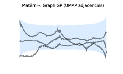
Figure 6: Samples of $\mathbf{y}$ plotted against $\mathbf{X}$, using a generative model,
$\mathbf{y}|\tilde{\mathbf{L}}\sim\mathcal{N}(\mathbf{0},\exp[-12.5\mathbf{L}]),$
$\tilde{\mathbf{L}}|\mathbf{A}^{\prime}=\mathbf{I}-\mathbf{D^{\dagger}}^{0}.5(\mathbf{A}^{\prime}+\mathbf{A}^{\prime T})\mathbf{D^{\dagger}}^{0}.5,$
$\forall i<j,\mathbf{A}_{ij}^{\prime}|\mathbf{X}\sim\text{Bernoulli}(1/(1+2\|\mathbf{X}_{i:}-\mathbf{X}_{j:}\|^{2}))$ and
$\mathbf{X}\sim\text{Uniform}(-3,3).$

Appendix D A mean-field EM perspective on the UMAP Generative Model

D.1 Model set-up

Assuming the model,

$$p(\mathbf{A^{\prime}}|\mathbf{X}) =\prod_{i<j}\text{Bernoulli}(\mathbf{A}_{ij}^{\prime}|\mathbf{\pi}_{ij})$$

$$\mathbf{A} =\mathbf{A^{\prime}}+\mathbf{A^{\prime}}^{T}$$

$$p(\mathbf{Y}|\mathbf{A}) =\mathcal{N}(\mathbf{Y}|0,(\mathbf{L}+\beta\mathbf{I})^{-1})$$

The likelihood in this model can be written as:

$$p(\mathbf{Y}|\mathbf{A})=\frac{\left|\beta\mathbf{I}+\mathbf{L}\right|^{\frac{d}{2}}}{\left(2\pi\right)^{\frac{dn}{2}}}\exp\left(\frac{1}{2}\text{Tr}\left(\mathbf{Y}\mathbf{Y}^{\top}\left(\beta\mathbf{I}+\mathbf{L}\right)\right)\right)$$ (6)

where $\mathbf{Y}\in\mathbb{R}^{n\times d}$ is our data in the form of a design matrix with $p$ features and $n$ data points. Define:

$$\mathbf{L}=\rho\bm{\Phi}\mathbf{A_{d}}\bm{\Phi}^{\top},$$

where

$$\bm{\Phi}=\left(\mathbf{1}^{\top}\otimes\mathbf{I}-\mathbf{I}\otimes\mathbf{1}^{\top}\right)\in\mathbb{R}^{n\times n^{2}}$$

and

$$\mathbf{A_{d}}\in\mathbb{R}^{n^{2}\times n^{2}}$$

and has diagonal elements, where the $k$th diagonal is given by $\mathbf{A}_{ij}$ where $k=i+n(j-1)$, and we constrain $\mathbf{A}_{ii}=0$ and $\mathbf{A}_{ij}=\mathbf{A}_{ji}$ and $\mathbf{A}_{ij}$ is either zero or one.

We introduce a mean-field variational distribution on $\mathbf{A}$:

$$q(\mathbf{A})=\prod_{i<j}q(\mathbf{A}_{ij}).$$

Following Blei et al. (2017), as part of mean-field variational inference, for every edge $ij$, we set $q(\mathbf{A}_{ij})$ proportional to:

$$q\left(\mathbf{A}_{ij}\right)\propto\exp[\mathbb{E}_{\mathbf{A_{-ij}}}(\log p(\mathbf{Y}\mid\mathbf{A})+\log p(\mathbf{A}))].$$

To write out these probabilities as an expectation given edges apart from $ij$, we formulate the determinant and trace terms in Equation 6,

D.2 Calculating the Determinant

The determinant can be calculated as:

$$\begin{gathered}|\beta\mathbf{I}+\mathbf{L}|^{\frac{d}{2}}=\left|\beta\mathbf{I}+\rho\bm{\Phi}\mathbf{A}\bm{\Phi}^{\top}\right|^{\frac{d}{2}}\end{gathered}$$

$$=\left|\beta\mathbf{I}+\hat{\mathbf{L}}_{ij}+\mathbf{A}_{ij}\rho\bm{\phi}_{:,ij}\bm{\phi}_{:,ij}^{\top}+\mathbf{A}_{ji}\rho\bm{\phi}_{:,ji}\bm{\phi}_{:,ji}^{\top}\right|^{\frac{d}{2}}$$

$$=\left|\beta\mathbf{I}+\hat{\mathbf{L}}_{ij}\right|^{\frac{d}{2}}\left(1+2\mathbf{A}_{ij}\rho\bm{\phi}_{:,ij}{}^{\top}\left(\beta\mathbf{I}+\hat{\mathbf{L}}_{ij}\right)^{-1}\bm{\phi}_{:,ij}\right)^{\frac{d}{2}}$$

$$=\left|\beta\mathbf{I}+\hat{\mathbf{L}}^{ij}\right|^{\frac{d}{2}}\left(1+2\mathbf{A}_{ij}\rho\bm{\phi}_{:,ij}{}^{\top}\hat{\mathbf{C}}^{ij}\bm{\phi}_{:,ij}\right)^{\frac{d}{2}}$$

where $\hat{\mathbf{L}}^{ij}$ corresponds to the graph Laplacian with edge $ij$ removed and $\hat{\mathbf{C}}^{ij}=\left(\beta\mathbf{I}+\hat{\mathbf{L}}^{ij}\right)^{-1}$ is the cavity covariance, i.e. the covariance of $p(\mathbf{Y}|\mathbf{A})$ if we remove edge $i,j$. Now we note that

$$\phi_{:,ij}^{\top}\hat{\mathbf{C}}^{ij}\phi_{:,ij}=\hat{c}^{ij}_{i,i}+\hat{c}^{ij}_{j,j}-2\hat{c}^{ij}_{ij}=\kappa_{ij}.$$

where $\kappa_{ij}$ is the squared distance between the $i^{\text{th}}$ and $j^{\text{th}}$ point under the Gaussian governed by the cavity covariance.

D.3 Calculating the Trace

The trace term can be calculated as,

$$-\frac{1}{2}\operatorname{Tr}\left(\mathbf{Y}\mathbf{Y}^{\top}(\beta\mathbf{I}+\mathbf{L})\right)$$

$$=-\frac{1}{2}\beta\operatorname{Tr}\left(\mathbf{Y}\mathbf{Y}^{\top}\right)-\frac{\rho}{2}\operatorname{Tr}\left(\mathbf{Y}\mathbf{Y}^{\top}\bm{\Phi}\mathbf{A}\mathbf{\Phi}^{\top}\right)$$

$$=-\frac{1}{2}\beta\operatorname{Tr}\left(\mathbf{Y}\mathbf{Y}^{\top}\right)-\frac{1}{2}\operatorname{Tr}\left(\mathbf{Y}\mathbf{Y}^{\top}\hat{\mathbf{L}}^{ij}\right)-\mathbf{A}_{ij}\rho d_{ij}$$

where

$$d_{ij}=\left(\mathbf{y}_{i,:}^{\top}\mathbf{y}_{i,:}-2\mathbf{y}_{i,:}^{\top}\mathbf{y}_{j,:}+\mathbf{y}_{j,:}^{\top}\mathbf{y}_{j,:}\right).$$

D.4 Mean-field EM Perspective

In this section, we describe an EM update step implied by assuming the model in Equation 6.

For approximate EM, we assume a mean field approximation for our distribution $q(\mathbf{A})=\prod_{i=1}^{n}\prod_{j<i}^{n}q(\mathbf{A}_{ij})$. By substituting the forms of the determinant and trace computed above (that split up the terms into terms that involve $\mathbf{A}_{ij}$ and terms that don’t), we arrive at the equation below (ignoring terms that don’t depend on $\mathbf{A}_{ij}$),

$$q(\mathbf{A}_{ij})\propto\exp[\mathbb{E}_{\mathbf{A_{-ij}}}(\log(1+2\mathbf{A}_{ij}\rho\kappa_{ij})^{\frac{d}{2}})-\mathbf{A}_{ij}\rho d_{ij}+\mathbf{A}_{ij}\log\pi_{ij}^{(k-1)}-\mathbf{A}_{ij}\log(1-\pi_{ij}^{(k-1)})].\;$$ (7)

As $d\rightarrow\infty$, and setting $\rho=1/d$,

$$\log(1+2\mathbf{A}_{ij}\rho\kappa_{ij})^{\frac{d}{2}}\longrightarrow\log\exp\mathbf{A}_{ij}\kappa_{ij},$$

and so the variational probabilities are approximately proportional to,

$$q(\mathbf{A}_{ij})\propto\exp[\mathbf{A}_{ij}\mathbb{E}_{\mathbf{A_{-ij}}}(\kappa_{ij})-\mathbf{A}_{ij}\rho d_{ij}+\mathbf{A}_{ij}\log\pi_{ij}^{(k-1)}-\mathbf{A}_{ij}\log(1-\pi_{ij}^{(k-1)})],$$

$$q(\mathbf{A}_{ij})\propto\exp\left[\mathbf{A}_{ij}\left[\mathbb{E}_{\mathbf{A_{-ij}}}(\kappa_{ij})-\dfrac{d_{ij}}{d}+\log\dfrac{\pi_{ij}^{(k-1)}}{1-\pi_{ij}^{(k-1)}}\right]\right].$$

Because $\mathbf{A}_{ij}$ can only be zero or one (and hence have a Bernoulli distribution), we obtain,

$$q(\mathbf{A}_{ij}=1) =\frac{\exp\left[\mathbb{E}_{\mathbf{A_{-ij}}}(\kappa_{ij})-\dfrac{d_{ij}}{d}+\log\dfrac{\pi_{ij}^{(k-1)}}{1-\pi_{ij}^{(k-1)}}\right]}{1+\exp\left[\mathbb{E}_{\mathbf{A_{-ij}}}(\kappa_{ij})-\dfrac{d_{ij}}{d}+\log\dfrac{\pi_{ij}^{(k-1)}}{1-\pi_{ij}^{(k-1)}}\right]}$$

$$=\sigma\left(\left[\mathbb{E}_{\mathbf{A_{-ij}}}(\kappa_{ij})-\dfrac{d_{ij}}{d}+\sigma^{-1}(\pi_{ij}^{(k-1)})\right]\right).$$

Using these results as part of the coordinate ascent variational inference (CAVI, Blei et al. (2017)), results in an expectation (E) update step,

$$\forall i\neq j:q^{k+1}(\mathbf{A}_{ij}=1)=\pi_{ij}^{(k+1)}=\sigma\left(\left[\mathbb{E}_{\mathbf{A_{-ij}}}(\kappa_{ij})-\dfrac{d_{ij}}{d}+\sigma^{-1}(\pi^{k}_{ij})\right]\right).$$

Note that in the MFVI setting $q^{k+1}(\mathbf{A}_{ij}=1)=\pi_{ij}^{(k+1)}$ as this brings the second term in Equation 2 to 0. We believe that the term $\mathbb{E}_{\mathbf{A_{-ij}}}(\kappa_{ij})$ approximates $d_{ij}/d$ for large $d$ due to Lemma B.27. We hope that this framework allows for future research with the specified model methodology.

Appendix E Alternative generative models

Here, we describe other potential generative models that can be specified given an adjacency matrix $\mathbf{A}$.

E.1 Gaussian Bayesian Networks

Murphy (2012) describes the joint distribution of a Gaussian directed acyclical graphical model, providing a generative model for our framework. It appears as,

$$\mathbf{Y} \sim\mathcal{MN}(0,\mathbf{M}\mathbf{M}^{T},\mathbf{I}),$$

where $\mathbf{M}$ is a lower triangular matrix (the Cholesky decomposition of the covariance) such that $\mathbf{M}=(\mathbf{I}-\mathbf{A})^{-1}$ and $\mathbf{A}$ is a row-normalised lower triangular adjacency matrix. This generative model is equivalent to:

$$\mathbf{Y}_{ij}|\text{pa}(i)\sim\mathcal{N}\left(\frac{1}{|\text{pa}(i)|}\sum_{k\in\text{pa}(i)}\mathbf{Y}_{kj},1\right),$$

where $\text{pa}(i)$ is the set of points that are parents to point $i$, and $|.|$ denotes the size of a set.

E.2 Graph Convolutional Gaussian Processes

The graph convolutional Gaussian process (GCGP), described in Opolka and Liò (2020); Ng et al. (2018), is defined as

$$\mathbf{Y}\sim\mathcal{MN}(0,\mathbf{S}^{k}\mathbf{C}[\mathbf{S}^{k}]^{T},\mathbf{I}),$$

where $\mathbf{C}$ is a kernel matrix, $\mathbf{S}^{k}$ is a normalized adjacency matrix defined using $\tilde{\mathbf{A}}=\mathbf{A}+\mathbf{I}$, raised to the $k$-th power. Taking $\mathbf{C}$ to be an identity matrix provides a potential generative model for our framework.

Note that due to the Neumann expansion, the Cholesky decomposition of the covariance in Section E.1 can be written as,

$$\mathbf{M}=(\mathbf{I}-\tilde{\mathbf{A}}^{T})^{-1}=\sum_{k=0}^{\infty}(\tilde{\mathbf{A}}^{T})^{k}.$$

This shows that a sum of GCGPs (using increasing powers of the adjacency matrix, without self edges) approximates the covariance in Section E.1 when the graph is a DAG. The expansion also shows that the covariance of Section E.1 is composed of all possible hops in the graph, as powers of an adjacency matrix have the interpretation of storing the number of paths from each node to another (Barber, 2012).

Appendix F Connections to other work

The proposed framework could be changed by directly specifying a generative model on data $\mathbf{Y}$ conditioning on latent variables $\mathbf{X}$ and a further set of latent variables $\mathbf{X}^{\prime}$ that don’t affect $\mathbf{A}^{\prime}$ directly. This is illustrated in Figure 7. Motivations to do this include improving the separation of clusters of points that belong to different labels (e.g. cell types) in recovered embeddings by a GPLVM or a VAE, which (t-)SNE and UMAP can be more performant at.

Figure 7: Class of possible extensions of the framework, where latent variables $\mathbf{X}$ and a further set of latent variables $\mathbf{X}^{\prime}$ that don’t affect $\mathbf{A}^{\prime}$ may be used to describe the distribution of $\mathbf{Y}$ directly. Dashed edges show connections that may or may not be added and greyed nodes show observed random variables or parameters.

In such models, the ELBO is given by,

$$\mathcal{L}=\; \mathbb{E}_{q(\mathbf{A}^{\prime}|\mathbf{Y})q(\mathbf{X})q(\mathbf{X}^{\prime})}[\log p(\mathbf{Y}|\mathbf{A}^{\prime},\mathbf{X}^{\prime},\mathbf{X})]$$

$$- \text{KL}(q(\mathbf{A}^{\prime}|\mathbf{Y})||p(\mathbf{A}^{\prime}|\mathbf{X}))$$

$$- \text{KL}(q(\mathbf{X}|\mathbf{Y})||p(\mathbf{X}))$$

$$- \text{KL}(q(\mathbf{X}^{\prime})||p(\mathbf{X}^{\prime})).$$

Such objectives, where a t-SNE/UMAP style loss is added to that of another model (e.g. scvis (Ding et al., 2018) and GPLVMs with t-SNE objectives (van der Maaten, 2009)), and models that use neural networks for amortised inference of $\mathbf{X}$, appear frequently in literature.

References

- Ahmed et al. (2018) Sumon Ahmed, Magnus Rattray, and Alexis Boukouvalas. GrandPrix: scaling up the Bayesian GPLVM for single-cell data. Bioinformatics, 35(1):47–54, 07 2018. ISSN 1367-4803. 10.1093/bioinformatics/bty533. URL https://doi.org/10.1093/bioinformatics/bty533.
- Barber (2012) D. Barber. Bayesian Reasoning and Machine Learning. Cambridge University Press, 2012.
- Becht et al. (2019) Etienne Becht, Leland McInnes, John Healy, Charles-Antoine Dutertre, Immanuel W. H. Kwok, Lai Guan Ng, Florent Ginhoux, and Evan W. Newell. Dimensionality reduction for visualizing single-cell data using UMAP. Nature Biotechnology, 37(1):38–44, Jan 2019. ISSN 1546-1696. 10.1038/nbt.4314. URL https://doi.org/10.1038/nbt.4314.
- Belkin and Niyogi (2001) Mikhail Belkin and Partha Niyogi. Laplacian eigenmaps and spectral techniques for embedding and clustering. In T. Dietterich, S. Becker, and Z. Ghahramani, editors, Advances in Neural Information Processing Systems, volume 14. MIT Press, 2001. URL https://proceedings.neurips.cc/paper_files/paper/2001/file/f106b7f99d2cb30c3db1c3cc0fde9ccb-Paper.pdf.
- Belkin and Niyogi (2008) Mikhail Belkin and Partha Niyogi. Towards a theoretical foundation for laplacian-based manifold methods. Journal of Computer and System Sciences, 74(8):1289–1308, 2008. ISSN 0022-0000. https://doi.org/10.1016/j.jcss.2007.08.006. URL https://www.sciencedirect.com/science/article/pii/S0022000007001274. Learning Theory 2005.
- Blei et al. (2017) David M. Blei, Alp Kucukelbir, and Jon D. McAuliffe. Variational inference: A review for statisticians. Journal of the American Statistical Association, 112(518):859–877, 2017. 10.1080/01621459.2017.1285773. URL https://doi.org/10.1080/01621459.2017.1285773.
- Borg and Groenen (1997) Ingwer Borg and Patrick Groenen. Classical Scaling, pages 207–212. Springer New York, New York, NY, 1997. ISBN 978-1-4757-2711-1. 10.1007/978-1-4757-2711-1_12. URL https://doi.org/10.1007/978-1-4757-2711-1_12.
- Borovitskiy et al. (2021) Viacheslav Borovitskiy, Iskander Azangulov, Alexander Terenin, Peter Mostowsky, Marc Peter Deisenroth, and Nicolas Durrande. Matérn Gaussian processes on graphs, 2021.
- Borovitskiy et al. (2022) Viacheslav Borovitskiy, Alexander Terenin, Peter Mostowsky, and Marc Peter Deisenroth. Matérn gaussian processes on riemannian manifolds, 2022.
- Bui and Turner (2015) Thang D. Bui and Richard E. Turner. Stochastic variational inference for gaussian process latent variable models using back constraints. In Black Box Learning and Inference NIPS workshop, 2015.
- Coifman and Lafon (2006) Ronald R. Coifman and Stéphane Lafon. Diffusion maps. Applied and Computational Harmonic Analysis, 21(1):5–30, 2006. ISSN 1063-5203. https://doi.org/10.1016/j.acha.2006.04.006. URL https://www.sciencedirect.com/science/article/pii/S1063520306000546. Special Issue: Diffusion Maps and Wavelets.
- Ding et al. (2018) Jiarui Ding, Anne Condon, and Sohrab P. Shah. Interpretable dimensionality reduction of single cell transcriptome data with deep generative models. Nature Communications, 9(1):2002, May 2018. ISSN 2041-1723. 10.1038/s41467-018-04368-5. URL https://doi.org/10.1038/s41467-018-04368-5.
- Gelman et al. (2013) Andrew Gelman, John B. Carlin, Hal S. Stern, David B. Dunson, Aki Vehtari, and Donald B. Rubin. Bayesian Data Analysis. Chapman and Hall/CRC, 2013.
- Ghahramani (2015) Zoubin Ghahramani. Probabilistic machine learning and artificial intelligence. Nature, 521(7553):452–459, May 2015. ISSN 1476-4687. 10.1038/nature14541. URL https://doi.org/10.1038/nature14541.
- Hinton and Roweis (2002) Geoffrey Hinton and Sam Roweis. Stochastic neighbor embedding. In Proceedings of the 15th International Conference on Neural Information Processing Systems, NIPS’02, page 857–864, Cambridge, MA, USA, 2002. MIT Press.
- Ho et al. (2020) Jonathan Ho, Ajay Jain, and Pieter Abbeel. Denoising diffusion probabilistic models, 2020.
- Jordan (2009) Michael I. Jordan. The exponential family: Basics. 2009. URL https://people.eecs.berkeley.edu/~jordan/courses/260-spring10/other-readings/chapter8.pdf.
- Jordan et al. (1999) Michael I. Jordan, Zoubin Ghahramani, Tommi S. Jaakkola, and Lawrence K. Saul. An introduction to variational methods for graphical models. Machine Learning, 37(2):183–233, Nov 1999. 10.1023/A:1007665907178. URL https://doi.org/10.1023/A:1007665907178.
- Kingma and Welling (2014) Diederik P. Kingma and Max Welling. Auto-encoding variational Bayes, 2014.
- Lalchand et al. (2022a) Vidhi Lalchand, Aditya Ravuri, Emma Dann, Natsuhiko Kumasaka, Dinithi Sumanaweera, Rik G. H. Lindeboom, Shaista Madad, Sarah A. Teichmann, and Neil D. Lawrence. Modelling technical and biological effects in scRNA-seq data with scalable GPLVMs, 2022a.
- Lalchand et al. (2022b) Vidhi Lalchand, Aditya Ravuri, and Neil D Lawrence. Generalised gplvm with stochastic variational inference. In International Conference on Artificial Intelligence and Statistics, pages 7841–7864. PMLR, 2022b.
- Lawrence (2005) Neil D. Lawrence. Probabilistic non-linear principal component analysis with Gaussian process latent variable models. J. Mach. Learn. Res., 6:1783–1816, dec 2005. ISSN 1532-4435.
- Lawrence (2012) Neil D. Lawrence. A unifying probabilistic perspective for spectral dimensionality reduction: Insights and new models. J. Mach. Learn. Res., 13(1):1609–1638, may 2012. ISSN 1532-4435.
- Lawrence and Quiñonero Candela (2006) Neil D. Lawrence and Joaquin Quiñonero Candela. Local distance preservation in the gp-lvm through back constraints. In Proceedings of the 23rd International Conference on Machine Learning, ICML ’06, page 513–520, New York, NY, USA, 2006. Association for Computing Machinery. ISBN 1595933832. 10.1145/1143844.1143909. URL https://doi.org/10.1145/1143844.1143909.
- Mao et al. (2015) Qi Mao, Li Wang, Steve Goodison, and Yijun Sun. Dimensionality reduction via graph structure learning. In Proceedings of the 21th ACM SIGKDD International Conference on Knowledge Discovery and Data Mining, KDD ’15, page 765–774, New York, NY, USA, 2015. Association for Computing Machinery. ISBN 9781450336642. 10.1145/2783258.2783309. URL https://doi.org/10.1145/2783258.2783309.
- McInnes et al. (2020) Leland McInnes, John Healy, and James Melville. UMAP: Uniform manifold approximation and projection for dimension reduction, 2020.
- Murphy (2012) Kevin P. Murphy. Machine learning: a probabilistic perspective. 2012.
- Murphy (2023) Kevin P. Murphy. Probabilistic Machine Learning: Advanced Topics. MIT Press, 2023. URL http://probml.github.io/book2.
- Ng et al. (2018) Yin Cheng Ng, Nicolò Colombo, and Ricardo Silva. Bayesian semi-supervised learning with graph gaussian processes. In S. Bengio, H. Wallach, H. Larochelle, K. Grauman, N. Cesa-Bianchi, and R. Garnett, editors, Advances in Neural Information Processing Systems, volume 31. Curran Associates, Inc., 2018. URL https://proceedings.neurips.cc/paper_files/paper/2018/file/1fc214004c9481e4c8073e85323bfd4b-Paper.pdf.
- Nickel and Kiela (2017) Maximilian Nickel and Douwe Kiela. Poincaré embeddings for learning hierarchical representations, 2017.
- Opolka and Liò (2020) Felix L. Opolka and Pietro Liò. Graph convolutional Gaussian processes for link prediction, 2020.
- Stachenfeld et al. (2017) Kimberly L. Stachenfeld, Matthew M. Botvinick, and Samuel J. Gershman. The hippocampus as a predictive map. Nature Neuroscience, 20(11):1643–1653, Nov 2017. ISSN 1546-1726. 10.1038/nn.4650. URL https://doi.org/10.1038/nn.4650.
- Stan Development Team (2023) Stan Development Team. Stan modeling language users guide and reference manual 2.31, 2023. URL https://mc-stan.org.
- Tasic et al. (2018) Bosiljka Tasic, Zizhen Yao, Lucas T. Graybuck, Kimberly A. Smith, Thuc Nghi Nguyen, Darren Bertagnolli, Jeff Goldy, Emma Garren, Michael N. Economo, Sarada Viswanathan, Osnat Penn, Trygve Bakken, Vilas Menon, Jeremy Miller, Olivia Fong, Karla E. Hirokawa, Kanan Lathia, Christine Rimorin, Michael Tieu, Rachael Larsen, Tamara Casper, Eliza Barkan, Matthew Kroll, Sheana Parry, Nadiya V. Shapovalova, Daniel Hirschstein, Julie Pendergraft, Heather A. Sullivan, Tae Kyung Kim, Aaron Szafer, Nick Dee, Peter Groblewski, Ian Wickersham, Ali Cetin, Julie A. Harris, Boaz P. Levi, Susan M. Sunkin, Linda Madisen, Tanya L. Daigle, Loren Looger, Amy Bernard, John Phillips, Ed Lein, Michael Hawrylycz, Karel Svoboda, Allan R. Jones, Christof Koch, and Hongkui Zeng. Shared and distinct transcriptomic cell types across neocortical areas. Nature, 563(7729):72–78, Nov 2018. ISSN 1476-4687. 10.1038/s41586-018-0654-5. URL https://doi.org/10.1038/s41586-018-0654-5.
- Tenenbaum et al. (2000) Joshua B. Tenenbaum, Vin de Silva, and John C. Langford. A global geometric framework for nonlinear dimensionality reduction. Science, 290(5500):2319–2323, 2000. 10.1126/science.290.5500.2319. URL https://www.science.org/doi/abs/10.1126/science.290.5500.2319.
- Tipping and Bishop (1999) Michael E. Tipping and Christopher M. Bishop. Probabilistic principal component analysis. Journal of the Royal Statistical Society: Series B (Statistical Methodology), 61(3):611–622, 1999. https://doi.org/10.1111/1467-9868.00196. URL https://rss.onlinelibrary.wiley.com/doi/abs/10.1111/1467-9868.00196.
- Uhlig (1994) Harald Uhlig. On Singular Wishart and Singular Multivariate Beta Distributions. The Annals of Statistics, 22(1):395 – 405, 1994. 10.1214/aos/1176325375. URL https://doi.org/10.1214/aos/1176325375.
- van der Maaten (2009) Laurens van der Maaten. Preserving local structure in Gaussian process latent variable models. In Proceedings of the 18th Annual Belgian-Dutch Conference on Machine Learning, pages 81–88. Citeseer, 2009.
- van der Maaten and Hinton (2008) Laurens van der Maaten and Geoffrey Hinton. Visualizing data using t-SNE. Journal of Machine Learning Research, 9(86):2579–2605, 2008. URL http://jmlr.org/papers/v9/vandermaaten08a.html.
- von Luxburg (2007) Ulrike von Luxburg. A tutorial on spectral clustering. Statistics and Computing, 17(4):395–416, Dec 2007. ISSN 1573-1375. 10.1007/s11222-007-9033-z. URL https://doi.org/10.1007/s11222-007-9033-z.
- Weinberger et al. (2004) Kilian Q Weinberger, Fei Sha, and Lawrence K Saul. Learning a kernel matrix for nonlinear dimensionality reduction. In Proceedings of the twenty-first international conference on Machine learning, page 106, 2004.
- Williams and Agakov (2002) Christopher K. I. Williams and Felix V. Agakov. Products of Gaussians and Probabilistic Minor Component Analysis. Neural Computation, 14(5):1169–1182, 05 2002. ISSN 0899-7667. 10.1162/089976602753633439. URL https://doi.org/10.1162/089976602753633439.
- Zhu et al. (2014) Jun Zhu, Ning Chen, and Eric P. Xing. Bayesian inference with posterior regularization and applications to infinite latent svms, 2014.
- Zhu et al. (2003) Xiaojin Zhu, John Lafferty, and Zoubin Ghahramani. Semi-supervised learning: From Gaussian fields to Gaussian processes. School of Computer Science, Carnegie Mellon University, 2003.