Can ChatGPT Forecast Stock Price Movements? Return Predictability and Large Language Models

Abstract

We examine the potential of ChatGPT and other large language models in predicting stock market returns using news headlines. We use ChatGPT to assess whether each headline is good, bad, or neutral for firms’ stock prices. We document a significantly positive correlation between ChatGPT scores and subsequent daily stock returns. We find that ChatGPT outperforms traditional sentiment analysis methods. More basic models such as GPT-1, GPT-2, and BERT cannot accurately forecast returns, indicating return predictability is an emerging capacity of complex language models. Long-short strategies based on ChatGPT-4 deliver the highest Sharpe ratio. Furthermore, we find predictability in both small and large stocks, suggesting market underreaction to company news. Predictability is stronger among smaller stocks and stocks with bad news, consistent with limits-to-arbitrage also playing an important role. Finally, we propose a new method to evaluate and understand the models’ reasoning capabilities. Overall, our results suggest that incorporating advanced language models into the investment decision-making process can yield more accurate predictions and enhance the performance of quantitative trading strategies.

Keywords: Large Language Models, ChatGPT, Machine Learning, Return Predictability, Textual Analysis
JEL Classification: C81, G11, G12, G18

1 Introduction

The application of generative artificial intelligence and large language models (LLMs) such as ChatGPT in various domains has gained significant traction recently, with numerous studies exploring their potential in diverse areas. In financial economics, however, using LLMs remains relatively uncharted territory, especially concerning their ability to predict stock market returns. On the one hand, as these models are general-purpose language models and not explicitly trained for stock return prediction, one may expect that they offer little value in predicting stock returns. On the other hand, to the extent that these models are trained using truly big text data and more capable of understanding the context of natural language, one could argue that they could be of value for processing textual information to predict stock returns. Thus, the performance of LLMs in predicting financial market movements is an open question. Our paper aims to fill this gap by studying the potential of LLMs in extracting the context from news headlines to predict stock returns.

It is well documented that stock returns are predictable at a daily horizon using news and trained algorithms ([40], [42], and [41], among others), possibly because combining new information is complicated ([19]). Instead, our focus is to evaluate whether LLMs not trained in predicting returns acquire this capability as they become better at other natural language tasks and, if yes, how they compare to the commonly used methods in the finance literature. To the best of our knowledge, this paper is among the first to address these critical questions by evaluating the capabilities of LLMs in forecasting stock market returns. Through a novel approach that leverages the model’s sentiment analysis capabilities, we assess the performance of various LLMs, including ChatGPT, using news headlines data and compare it to existing sentiment analysis methods provided by leading data vendors.

To conduct our analysis, we first obtain daily stock returns for all US common stocks from the CRSP database and then construct a comprehensive data set of news headlines relevant to these stocks from major news media and newswires. Our sample period begins in October 2021 (as ChatGPT’s training data stops in September 2021) and ends in December 2022. This ensures that our evaluation is based on information not present in the model’s training data, allowing for a more accurate assessment of its predictive capabilities. For each headline, we use ChatGPT to assess whether it is good, bad, or neutral for firms’ stock prices. We convert these responses to numerical scores and use them to predict stock returns on the next trading day. We document a significantly positive correlation between ChatGPT scores and subsequent daily stock returns. For instance, without considering transaction costs, a self-financing strategy that buys the stocks with a positive ChatGPT score and sells stocks with a negative ChatGPT score after the news announcement earns a cumulative return of over 500% from 2021m10 – 2022m12.

Notably, the advanced capabilities of ChatGPT enable it to outpace traditional sentiment analysis methods in predicting stock returns. In particular, we compare the performance of ChatGPT scores to sentiment scores based on traditional methods, such as the sentiment score provided by a leading data vendor. When we include both scores in the same regressions, only the coefficient on ChatGPT’s score is positive and significant, while the coefficient on the data vendor’s score is insignificant. This suggests that state-of-the-art LLMs like ChatGPT fare well against traditional methods as they can better capture the context of the news headlines for stock market predictions.

Comparing the performance of various language models, we find that more basic models like GPT-1, GPT-2, and BERT display little stock forecasting capabilities. When we use these models to assess the news headlines, we do not find their scores to have any significantly positive correlation with subsequent stock returns. In contrast, we observe the highest predictability in the more complex models like ChatGPT-4. A self-financing strategy that buys the stocks with a positive ChatGPT-4 score and sells stocks with a negative ChatGPT-4 score after the news announcement delivers the highest Sharpe ratio (3.8) over our sample period, compared to a Sharpe ratio of 3.1 for the strategy based on ChatGPT-3.5.

Furthermore, we find that the predictability of the ChatGPT scores is present among both small and large-cap stocks as well as stocks with positive and negative news. Our results suggest that the market appears to be underreacting to company news at the frequency we examine, consistent with the evidence in the extant literature (e.g., [6], [13], and [30]). Nevertheless, the predictability is more pronounced among smaller stocks. For instance, the coefficient on the ChatGPT score in predicting returns of small stocks (i.e., less than the 10th percentile NYSE market cap distribution) is more than four times the magnitude of the one for the remaining sample. In addition, stocks with negative news headlines also show stronger predictability. Both observations are consistent with the idea that limits-to-arbitrage also play an essential role in driving this predictability.

Moreover, in light of our findings, we propose a new method to evaluate and understand the models’ reasoning capabilities. Our approach proceeds in several steps and takes advantage of these models’ ability to explain their reasoning. First, we evaluate whether the recommendations (excluding the neutral ones) were correct by comparing them with the realized return the following day. Second, we fit a model that predicts whether a recommendation is correct or incorrect using the recommendation reason. Third, we use the model’s feature importance to understand which concepts are better at predicting correct recommendations. We do so by looking at the most important words and their surrounding context. We find that the answers more likely to be correct are when the reasoning is related to stock purchases by insiders, earning guidance, and dividends. On the contrary, the model does worse when its reasoning relates to partnerships and developments.

Our findings have important implications for the employment landscape in the financial industry. The results could potentially lead to a shift in the methods used for market prediction and investment decision-making. By demonstrating the value of ChatGPT in financial economics, we aim to contribute to the understanding of LLMs’ applications in this field and inspire further research on integrating artificial intelligence and natural language processing in financial markets. In addition to the implications for employment in the financial industry, our study offers several other significant contributions.

First, our research can help regulators and policymakers understand the potential benefits and risks associated with the increasing adoption of LLMs in financial markets. As these models become more prevalent, their influence on market behavior, information dissemination, and price formation will become critical areas of concern. Our findings can inform discussions on regulatory frameworks that govern the use of AI in finance and contribute to the development of best practices for integrating LLMs into market operations.

Second, our study can benefit asset managers and institutional investors by providing empirical evidence on the efficacy of LLMs in predicting stock market returns. This insight can help these professionals make more informed decisions about incorporating LLMs into their investment strategies, potentially leading to improved performance and reduced reliance on traditional, more labor-intensive analysis methods.

Finally, our research contributes to the broader academic discourse on artificial intelligence applications in finance. By exploring the capabilities of ChatGPT in predicting stock market returns, we advance the understanding of LLMs’ potential and limitations within the financial economics domain. This can inspire future research on developing more sophisticated LLMs tailored to the financial industry’s needs, paving the way for more efficient and accurate financial decision-making. More broadly, our study has far-reaching implications that extend beyond the immediate context of stock market predictions. By shedding light on the potential contributions of ChatGPT to financial economics, we hope to encourage continued exploration and innovation in AI-driven finance.

Related Literature

Recent papers that use ChatGPT in the context of economics include [24], [16], [35], and [38]. [24] show that LLMs like ChatGPT can decode Fedspeak (i.e., the language used by the Fed to communicate on monetary policy decisions). [16] and [35] demonstrate that ChatGPT is helpful in teaching economics and conducting economic research. [38] find that ChatGPT can enhance productivity in professional writing jobs. Furthermore, [48] demonstrates that ChatGPT successfully identifies credible news outlets. Contemporaneously, [46] find ChatGPT is no better than simple methods such as linear regression when using numerical data in prediction tasks, and [34] try to use ChatGPT to help with a portfolio selection problem but find no positive performance. We attribute the difference in results to their focus on using historical numerical data to predict, while ChatGPT excels at textual tasks. Our study is among the first to study the potential of LLMs in financial markets, particularly the investment decision-making process.

We also contribute to the recent strand of the literature that employs textual analysis and machine learning to study a variety of finance research questions (e.g., [28], [39], [12], [27], [22], [5], [37], [25], [33], [32], [9], [29], [23], [15], [20], [36], [8], [10], [14]).

Our paper makes a unique contribution to this literature as it is the first to evaluate the capabilities of ChatGPT, a leading large language model, in forecasting stock returns - a critical and financially relevant prediction task it is not explicitly trained for. Rather than training it on finance data, we rely on ChatGPT’s natural language processing skills. We provide the first comprehensive evidence that ChatGPT can extract signals from news headlines to outperform traditional sentiment measures in predicting cross-sectional returns. Our approach directly tests the return forecasting abilities of modern AI systems, complementing behavioral finance studies focused on market inefficiencies. In addition, we also propose a novel evaluation technique to understand ChatGPT’s reasoning by predicting the correctness of the recommendations. This work substantially advances the emerging literature on interpreting complex models. Our paper delivers fundamental new insights into large language models’ stock return predictability skills, distinguishing it from concurrent research employing these models for asset allocation.

Our paper also adds the literature that uses linguistic analyses of news articles to extract sentiment and predict stock returns. One strand of this literature studies media sentiment and aggregate stock returns (e.g., [40], [21], [11]). Another strand of the literature uses the sentiment of firm news to predict future individual stock returns (e.g., [42], [41], [30]). Different from prior studies, we focus on understanding whether LLMs add value by extracting additional information that predicts stock market reactions.

Finally, our paper also relates to the literature on employment exposures and vulnerability to AI-related technology. Recent works by [3], [44], [1], [2], [4], [31], and [38] have examined the extent of job exposure and vulnerability to AI-related technology as well as the consequences for employment and productivity. With AI being on a constant rise since its inception, our study focuses on understanding an urgent but unanswered question—the capabilities of AI, and LLMs in particular, in the finance domain. We highlight the potential of LLMs in adding value to market participants in processing information to predict stock returns.

2 Institutional Background

ChatGPT is a large-scale language model developed by OpenAI based on the GPT (Generative Pre-trained Transformer) architecture. It is one of the most advanced natural language processing (NLP) models developed to date and trained on a massive corpus of text data to understand the structure and patterns of natural language. The Generative Pre-trained Transformer (GPT) architecture is a deep learning algorithm for natural language processing tasks. It was developed by OpenAI and is based on the Transformer architecture, which was introduced in [43]. The GPT architecture has achieved state-of-the-art performance in various natural language processing tasks, including language translation, text summarization, question answering, and text completion.

The GPT architecture uses a multi-layer neural network to model the structure and patterns of natural language. Using unsupervised learning methods, it is pre-trained on a large corpus of text data, such as Wikipedia articles or web pages. This pre-training process allows the model to develop a deep understanding of language syntax and semantics, which is then fine-tuned for specific language tasks. One of the unique features of the GPT architecture is its use of the transformer block, which enables the model to handle long sequences of text by using self-attention mechanisms to focus on the most relevant parts of the input. This attention mechanism allows the model to understand the input context better and generate more accurate and coherent responses.

ChatGPT has been trained to perform various language tasks such as translation, summarization, question answering, and even generating coherent and human-like text. ChatGPT’s ability to generate human-like responses has made it a powerful tool for creating chatbots and virtual assistants to converse with users. While ChatGPT is a powerful tool for general-purpose language-based tasks, it is not explicitly trained to predict stock returns or provide financial advice. Hence, we test its capabilities when predicting stock returns.

Although not explicitly trained in predicting asset prices, as a powerful natural language model exposed to massive text corpora, ChatGPT exhibits sophisticated reasoning skills and an aptitude for nuanced language comprehension. This ability to understand contextual meanings and linguistic patterns could enable ChatGPT to extract valuable signals about a firm’s prospects from textual data like news headlines, even without direct finance training. The model may identify subtle cues and compositional sentiment factors correlated with market reactions. We hypothesize that ChatGPT outperforms alternative sentiment measures in forecasting returns due to its more nuanced language comprehension capabilities. Further, we expect greater return predictability using ChatGPT versions with higher complexity, as they have greater representation power to process text. Economically, ChatGPT may be able to exploit investor underreaction to subtle signals in the news before subsequent price correction.

In addition to evaluating ChatGPT, we also assess the capabilities of other prominent natural language processing models, including GPT-1, GPT-2, BERT, and BART. GPT-1 was an early generative pre-trained transformer model introduced by OpenAI in 2018. It pioneered the use of attention mechanisms and transformers for natural language tasks. GPT-2, released in 2019, scaled up GPT-1 significantly, containing 10x more parameters. It demonstrated more powerful text generation abilities and language understanding than GPT-1.

BERT (Bidirectional Encoder Representations from Transformers) was developed by Google in 2018. Unlike GPT’s unidirectional training, BERT leverages bidirectional training of transformers, allowing the model to incorporate context from both directions. This distinguishes BERT from GPT-based models. BERT obtains state-of-the-art results on various NLP benchmarks and provides semantic representations useful for many downstream tasks. BART (Bidirectional and Auto-Regressive Transformer) builds on BERT with a sequence-to-sequence model architecture. Developed by Facebook in 2019, BART is pre-trained by reconstructing corrupted text, giving it strong text generation capabilities. The bidirectional encoder component allows BART to condition its generation on the surrounding context.

Bidirectional models like BERT and BART differ from autoregressive models like GPT in how they process context during training. BERT uses a bidirectional transformer encoder to incorporate contextual information from both directions. This allows it to condition predictions on the entire input sequence. However, the tradeoff is that BERT loses the generative modeling capabilities of GPT. Autoregressive models like GPT train in a unidirectional manner, modeling the probability distribution of the next token conditioned only on previous tokens. This sequential approach allows GPT to generate fluent and coherent text efficiently. The unidirectional conditioning enables strong generative abilities but with a more limited context window. In summary, BERT leverages bidirectional conditioning for broader context and superior prediction but lacks generative powers. GPT focuses on unidirectional autoregressive modeling to excel at text generation while having a more limited context window for prediction tasks. These models have shown success in diverse natural language tasks. However, they are less advanced than ChatGPT in scale and performance on benchmarks (e.g., [47]).

By evaluating the more basic models alongside ChatGPT, we can examine the importance of model complexity for stock return prediction based on textual data. Comparing ChatGPT to these foundational NLP models provides a more comprehensive view of the evolution of predictive capabilities with larger language models. In Appendix A, we provide an overview of the nine different LLMs that we study in this paper, ordered by their release date.

3 Data

We utilize three primary datasets for our analysis: the Center for Research in Security Prices (CRSP) daily returns, news headlines, and RavenPack. The sample period begins in October 2021 (as ChatGPT’s training data is available only until September 2021) and ends in December 2022. This sample period ensures that our evaluation is based on information not present in the model’s training data, allowing for a more accurate “out-of-sample” assessment of its predictive capabilities.

The CRSP daily returns dataset contains information on daily stock returns for a wide range of companies listed on major U.S. stock exchanges, including data on stock prices, trading volumes, and market capitalization. This comprehensive dataset enables us to examine the relationship between the sentiment scores generated by ChatGPT and the corresponding stock market returns. Our sample consists of all the stocks listed on the New York Stock Exchange (NYSE), the National Association of Securities Dealers Automated Quotations (NASDAQ), and the American Stock Exchange (AMEX), with at least one news story covered by a major news media or newswire. Following prior studies, we focus our analysis on common stocks with a share code of 10 or 11.

We first collect a comprehensive news dataset for all CRSP companies using web scraping. We search for all news containing either the company name or the ticker. The resulting dataset comprises news headlines from various sources, such as major news agencies, financial news websites, and social media platforms. For each company, we collect all news in the sample period. We then match the headlines with those from a prominent news sentiment analysis data provider (RavenPack). We match the period and the news title for all companies that have returns on the following market opening. Most (more than 70%) of matched headlines correspond to press releases. We do not use the RavenPack enhance headlines that potentially contain more information since they are not widely disseminated to the public. We match 67,586 headlines of 4,138 unique companies. We process the merged dataset using the preprocessing methods outlined by [30].

Importantly, matching with RavenPack assures that only relevant news will be used for the experiment. They closely monitor the major financial news distribution outlets and have a quality procedure matching news, timestamps, and entity names, which solves any errors that may have come from the web scraping procedure. Further, we employ their news categorization to explain the differences in return predictability across different models. Moreover, they have a close mapping with CRSP, which ensures the matching of the news and returns at the exact time. We further use their infrastructure by using only the information they consider highly relevant for a given company in a given period.

We employ the “relevance score” from the data vendor, which ranges from 0 to 100, to indicate how closely the news pertains to a specific company. A 0 (100) score implies that the entity is mentioned passively (predominantly). Our sample requires news stories with a relevance score of 100. We limit it to complete articles and press releases and exclude headlines categorized as ‘stock-gain’ and ‘stock-loss’ as they only indicate the daily stock movement direction. To avoid repeated news, we require the “event similarity days” to exceed 90, which ensures that only new information about a company is captured. These filters are imposed to ensure that we analyze fresh and relevant news headlines that could impact stock prices, which provides power to test the capabilities of LLMs in predicting stock market movements.

Furthermore, we eliminate duplicates and overly similar headlines for the same company on the same day. We gauge headline similarity using the Optimal String Alignment metric (the Restricted Damerau-Levenshtein distance) and remove headlines with a similarity greater than 0.6 for the same company on the same day. These filtering techniques do not introduce look-ahead bias, as the data vendor evaluates all news articles within milliseconds of receipt and promptly sends the resulting data to users. Consequently, all information is available at the time of news release.

Table 1 presents selected descriptive statistics of the sample: (i) the daily stock returns (%), (ii) the headline length, (iii) the response length, (iv) the GPT score (1 if ChatGPT 3.5 says YES, 0 if UNKNOWN, and -1 if NO), and the event sentiment score provided by the data vendor. The average GPT score is positive (0.24) with the median being zero and the event sentiment score shows a similar pattern. Thus, news headlines have an overall positive tilt. Panel B reports the correlation matrix of these variables. The correlation between the GPT score and event sentiment score is low, less than 0.28.

4 Methods

4.1 Prompt

Prompts are critical in guiding ChatGPT’s responses to specific tasks and queries. A prompt is a short text that provides context and instructions for ChatGPT to generate a response. The prompt can be as simple as a single sentence or as complex as a paragraph or more, depending on the nature of the task.

The prompt serves as the starting point for ChatGPT’s response generation process. The model uses the information contained in the prompt to generate a relevant and contextually appropriate response. This process involves analyzing the syntax and semantics of the prompt, developing a series of possible answers, and selecting the most appropriate one based on various factors, such as coherence, relevance, and grammatical correctness.

Prompts are essential for enabling ChatGPT to perform a wide range of language tasks, such as language translation, text summarization, question answering, and even generating coherent and human-like text. They allow the model to adapt to specific contexts and generate responses tailored to the user’s needs. Moreover, prompts can be customized to perform tasks in different domains, such as finance, healthcare, or customer support.

We use the following prompt in our study and apply it to the publicly available headlines.

Forget all your previous instructions. Pretend you are a financial expert. You are a financial expert with stock recommendation experience. Answer “YES” if good news, “NO” if bad news, or “UNKNOWN” if uncertain in the first line. Then elaborate with one short and concise sentence on the next line. Is this headline good or bad for the stock price of _company_name_ in the _term_ term?
Headline: _headline_

In this prompt, we ask ChatGPT, a language model, to assume the role of a financial expert with experience in stock recommendations. The terms _company_name_ and _headline_ are substituted by the firm name and the respective headline during the query. _term_ corresponds to either short or long-term. The prompt is specifically designed for financial analysis and asks ChatGPT to evaluate a given news headline and its potential impact on a company’s stock price in the short term. ChatGPT is requested to answer “YES” if the news is good for the stock price, “NO” if it is bad, or “UNKNOWN” if it is uncertain. ChatGPT is then asked to explain in one sentence to support its answer concisely. The prompt specifies that the news headline is the only source of information provided to ChatGPT. It is implicitly assumed that the headline contains sufficient information for an expert in the financial industry to reasonably assess its impact on the stock price. This prompt is designed to demonstrate the capabilities of ChatGPT as a language model in financial analysis tasks. We set the temperature of GPT models to 0 to maximize the reproducibility of the results.

For example, consider the following headline about Oracle:

Rimini Street Fined $630,000 in Case Against Oracle.

The prompt then asks:

Forget all your previous instructions. Pretend you are a financial expert. You are a financial expert with stock recommendation experience. Answer “YES” if good news, “NO” if bad news, or “UNKNOWN” if uncertain in the first line. Then elaborate with one short and concise sentence on the next line. Is this headline good or bad for the stock price of Oracle in the short term?
Headline: Rimini Street Fined $630,000 in Case Against Oracle

And here is ChatGPT’s response:

YES

The fine against Rimini Street could potentially boost investor confidence in Oracle’s ability to protect its intellectual property and increase demand for its products and services.

The news headline states that Rimini Street has been fined $630,000 in a case against Oracle. The proprietary software analytics tool gives a negative sentiment score of -0.52, indicating that the news is perceived as unfavorable. However, ChatGPT responds that it believes the information to be positive for Oracle. ChatGPT reasons that the fine could increase investor confidence in Oracle’s ability to protect its intellectual property, potentially leading to increased demand for its products and services. This difference in sentiment highlights the importance of context in natural language processing and the need to carefully consider the implications of news headlines before making investment decisions.

4.2 Empirical Design

We prompt ChatGPT to provide a recommendation for each headline and transform it into a numerical “ChatGPT score,” where “YES” is mapped to 1, “UNKNOWN” to 0, and “NO” to -1. We average the scores if there are multiple headlines for a company on a given day. We match the headlines to the next trading period. For headlines before 6 a.m. on a trading day, we assume the headlines can be traded by the market opening of the same day and sold at the close of the same day. For headlines after 6 a.m. but before 4 p.m., we assume the headlines can be traded at the same day’s close and sold at the close of the next trading day. For headlines after 4 p.m., we assume the headlines can be traded at the opening price of the next day and sold at the closing price of that next day. We then run linear regressions of the next day’s stock returns on the ChatGPT score, the sentiment score provided by the data vendor, and scores from other LLMs. Thus, all of our results are out-of-sample.

Specifically, we estimate the following regression specification:

$$r_{i,t+1}=a_{i}+b_{t}+\gamma^{\prime}x_{i,t}+\varepsilon_{i,t+1},$$ (1)

where the dependent variable, $r_{i,t+1}$, is stock $i$’s return over a subsequent trading day as discussed above, $x_{i,t}$ refers to the vector containing the ChatGPT score or other scores from assessing stock $i$’s news headlines, and $a_{i}$ and $b_{t}$ are firm and date fixed effects, respectively, which account for any observable and unobservable time-invariant firm characteristics and common time-specific factors that could influence stock returns. Standard errors are double clustered by date and firm.

In addition to analyzing the performance of ChatGPT, we examine the capabilities of other more basic models such as BERT, GPT-1, and GPT-2, and compare their performance with that of the more advanced models. For the more basic models, we employ a different strategy because those models cannot follow instructions or answer specific questions. For instance, GPT-1 and GPT-2 are auto-complete models. In Appendix B of the paper, we provide more details on the prompts we use for these models. Contrasting the performance of the basic vs. the more advanced LLMs allows us to shed light on whether return predictability is an emerging capacity of the recent developments in language models.

5 Results

5.1 Long-Short Strategies based on ChatGPT Scores

To assess ChatGPT’s capabilities to predict stock price movements, we start by examining the performance of long-short strategies formed based on ChatGPT scores of news headlines. In particular, we form zero-cost portfolios that buy the stocks with a positive ChatGPT score and sell stocks with a negative ChatGPT score after the news release. If a piece of news is released before 6 a.m. on a trading day, we enter the position at the market opening and exit at the close of the same day. If the news is released after 6 a.m. but before the market close, we enter the position at the market close price of the same day and exit at the close of the next trading day. If the news is announced after the market closes, we assume we enter the position at the next opening price and exit at the close of the next trading day. All strategies are rebalanced daily.

Figure 1 plots the cumulative returns of seven different trading strategies (investing $1) without considering transaction costs. These seven strategies include (1) an equal-weighted portfolio that buys companies with good news based on ChatGPT 3.5 (“Long”), (2) an equal-weighted portfolio that sells companies with bad news based on ChatGPT 3.5 (“Short”), (3) a self-financing long-short strategy based on ChatGPT 3.5 (“Long - Short”), (4) a self-financing long-short strategy based on ChatGPT 4 (“Long - Short GPT 4”), (5) an equal-weight market portfolio (Market Equally-Weighted), (6) a value-weight market portfolio (“Market Value-Weighted”), and (7) an equal-weight portfolio in all stocks with news the day before regardless of the news direction (“All News”).

We find strong evidence of the power of ChatGPT scores in predicting stock returns the next day. For instance, without considering transaction costs, a self-financing strategy that buys stocks with a positive ChatGPT-3.5 score and sells stocks with a negative ChatGPT-3.5 score earns an astonishing cumulative return of over 550% from 2021m10 – 2022m12. In contrast, the equal-weight and value-weight market portfolios and a naive equal-weight all-news portfolio all earn negative cumulative returns over the same periods. The sharp difference in performance across these two sets of portfolios demonstrates that as a leading LLM, ChatGPT can add value by extracting valuable information from news headlines that predicts stock market reactions. We note that both the long and short legs contribute to the predictability of ChatGPT. While the long leg delivers about 200%, the short leg delivers over 250%. Thus, the predictability is even stronger among stocks with bad news.

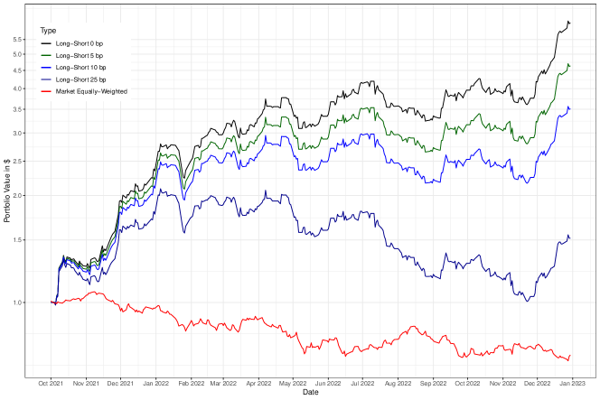
Figure 2: Cumulative Returns of Investing $1 in the Long-Short Strategy for Different Transaction Costs

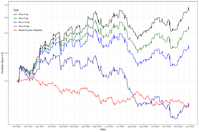
Figure 3: Cumulative Returns of Investing $1 in the Short Strategy for Different Transaction Costs

Obviously, one may argue that the analysis in Figure 1 ignores transaction costs and may or may not hold after incorporating transition costs. In Figure 2, we evaluate the performance of the long-short strategy based on ChatGPT 3.5 under different transaction cost assumptions: 5, 10, and 25 basis points (bps) per transaction. Even assuming a transaction cost of 5 bps per trade (i.e., 10 bps round-trip), the strategy still earns a cumulative return of over 450% during our sample period. As we increase the transaction costs to 10 bps per trade, the cumulative return is still as high as 350%. Assuming a very high transaction cost of 25 bps per trade, the cumulative return lowers to 50%. As the short leg tends to deliver higher cumulative returns, we evaluate its performance under different transaction cost assumptions in Figure 3. We find that the cumulative return of the short leg is more sensitive to transaction cost changes compared to the long-short portfolios. Increasing the transaction costs from 0 to 25 bps per trade will erode all the positive 250+% cumulative returns and make it negative and on par with the equal-weighted market portfolio.

Turning our attention to the more complex ChatGPT 4 model, the long-short strategy generates a cumulative return of over 350%, which also clearly outperforms the market portfolios or the naive all-news portfolio. While ChatGPT 4’s cumulative return is lower in magnitude compared to that of the long-short strategy based on ChatGPT 3.5, it has much lower variations over time.

In Table 2, we show the Sharpe ratio and maximum drawdown of the seven different strategies shown in Figure 1. We find that the strategy based on ChatGPT 4 delivers a much higher Sharpe ratio of 3.8, compared to a Sharpe ratio of 3.1 for the one based on ChatGPT 3.5. In addition, the ChatGPT 4 strategy has a maximum drawdown of -10.4% compared to the maximum drawdown of -22.8% for the ChatGPT 3.5 strategy. Thus, it appears that the predictability is better achieved by the more complex models like ChatGPT-4.

5.2 Results from Predictive Regressions

In this section, we use prediction regressions to evaluate the performance of different LLMs. Specifically, we carry out regressions as in Equation 1, using scores from different LLMs from assessing news headlines to predict next-day stock returns. Note that both firm and time fixed effects are included in the regressions, and standard errors are clustered by date and firm.

We present the results from regressions of stock returns on prediction scores from more advanced LLMs in Table 3. The main variables of interest include scores from three advanced LLMs: (i) ChatGPT 3.5, (ii) ChatGPT 4, and (iii) BART Large. We document several interesting findings. First, we find that the prediction score from ChatGPT 3.5 has a statistically and economically significant relation with the next-day stock returns. Specifically, the coefficient on ChatGPT 3.5’s score is 0.259 with a $t$-stat of 5.259. A switch from a negative (-1) to a positive (1) prediction score is associated with a 51.8 bps increase in next-day stock return. This result highlights the potential of ChatGPT as a valuable tool for predicting stock market movements based on sentiment analysis.

Second, we also compare the performance of ChatGPT with traditional sentiment analysis methods provided by the data vendor. In our analysis, we control for the ChatGPT sentiment scores and examine the predictive power of these alternative sentiment measures. Our results show that when controlling for the ChatGPT sentiment scores, the effect of the sentiment score from the data vendor on daily stock market returns is attenuated. This indicates that the ChatGPT model outperforms existing sentiment analysis methods in forecasting stock market returns.

The superiority of ChatGPT in predicting stock market returns can be attributed to its advanced language understanding capabilities, which allow it to capture the nuances and subtleties within news headlines. This enables the model to generate more reliable sentiment scores, leading to better predictions of daily stock market returns. These findings confirm the predictive power of ChatGPT sentiment scores and emphasize the potential benefits of incorporating LLMs into investment decision-making processes. By outperforming traditional sentiment analysis methods, ChatGPT demonstrates its value in enhancing the performance of quantitative trading strategies and providing a more accurate understanding of market dynamics.

Third, our analysis reveals that ChatGPT 4 sentiment scores also exhibit a strong and positive significant predictive power on daily stock market returns. Consistent with the evidence in Figure 1 and Table 2, the coefficient on the ChatGPT 4 score is lower than that of the ChatGPT 3.5 score, but the former has a large $t$-stat. Again, when we include both scores from ChatGPT 4 and the data vendor in the same regressions, only the coefficient on ChatGPT 4’s score is positive and significant, while the coefficient on the data vendor’s score is not.

To compare the performance of various language models, we further carry out a similar regression analysis using prediction scores from other LLMs. In particular, we consider six more basic LLMs in Table 4: (i) DistilBart-MNLI-12-1, (ii) GPT-2 Large, (iii) GPT-2, (iv) GPT-1, (v) BERT, and (vi) BERT Large. Our results show a striking pattern—return predictability is an emerging capacity of more complex language models. Scores from BART Large and DistilBart-MNLI models show some predictability but are noticeably weaker compared to ChatGPT 3.5 and 4. When we use more basic models such as GPT-1, GPT-2, and BERT to assess the news headlines, we do not find their scores to have any significantly positive correlation with subsequent stock returns. In contrast, we observe the highest predictability in the most complex model—ChatGPT-4.

In the next set of analyses, we examine the predictability of our full list of LLMs across small and large-cap stocks in Tables 5-8. Our results show that the predictability of the ChatGPT scores is present among both small and large-cap stocks. This suggests that the market appears to be underreacting to firm-specific news at the daily frequency we examine, consistent with the evidence in the long literature (e.g., [6], [13], [17], [26], and [30]). Nevertheless, we also find that the predictability is more pronounced among smaller stocks. For instance, the coefficient on the ChatGPT 3.5 score in predicting returns of small stocks (i.e., less than the 10th percentile NYSE market cap distribution) in Table 5 is more than four times the magnitude of the one for the remaining sample in Table 7 (0.653 with a t-stat of 5.145 vs 0.148 with a t-stat of 3.084). This observation is consistent with the idea that limits-to-arbitrage also play an essential role in driving this predictability.

Finally, we carry out more analysis to further understand the capabilities of the different LLMs in predicting stock market returns. Table 9 reports the average returns and abnormal returns based on the CAPM model and the 5-factor model of [18] for the different models. Panel A analyzes the full sample of common stocks, Panel B analyzes small stocks below the 10th percentile NYSE market capitalization, and Panel C analyzes the remaining non-small stocks. We find consistent evidence that more complex models are generally better. The magnitude and $t$-stat. of average returns and alphas are significantly higher for more advanced models like GPT-4 and GPT-3.5. For instance, the average daily return and the 5-factor alpha for GPT-4 are 44 bps ($t$-stat.=4.24) and 41 bps ($t$-stat.=4.01), respectively, which are both economically and statistically significant. In contrast, more basic models like GPT-1, GPT-2, and BERT do not generate significantly positive returns. This pattern holds for both small and large stocks.

Furthermore, Table 10 reports the Sharpe ratios and number of stocks in each leg by different models. As in the previous table, Panel A analyzes the full sample of common stocks, Panel B analyzes small stocks below the 10th percentile NYSE market capitalization, and Panel C analyzes the remaining non-small stocks. We find that while the long-short strategy based on GPT-3.5 generates higher average returns and alphas in terms of magnitude, it holds less diversified positions. For instance, as shown in Panel A, the average numbers of stocks in the short and long legs of the GPT-3.5 strategy are 3.8 and 50.9, respectively. The corresponding numbers for the GPT-4 strategy are 23.3 and 98.5, respectively, both of which are significantly higher than those for the GPT-3.5 strategy (more so for the short leg). As a result of a more diversified portfolio in both legs, the Sharpe ratio of the strategy based on GPT-4 is higher (3.8), compared to 3.1 of GPT-3.5. We find a consistent pattern that more complex models have higher Sharpe ratios. Importantly, the complex models continue to have a high Sharpe ratio in non-small stocks. For instance, as shown in Panel C, the Sharpe ratio for GPT-4 is as high as 2.99 even after removing the small stocks. Overall, the general ability of models to understand natural language appears to be positively correlated with their ability to accurately forecast returns.

6 Interpretability

6.1 Evaluating ChatGPT’s Reasoning Capabilities

Traditional machine learning models in finance primarily focus on prediction, often lacking interpretability. In contrast, large language models (LLMs) like ChatGPT offer predictions and associated explanations in natural language. This distinctive feature provides a deeper insight into the rationale behind each prediction, a capability largely absent in conventional models. Motivated by this unique attribute, we devise a novel framework to harness these qualitative insights for enhanced predictive accuracy. In our exploration of ChatGPT’s capabilities, every headline processed by the model yielded a prediction alongside an explanation. Unlike traditional quantitative models offering limited transparency, ChatGPT presents contextual reasoning in plain language, adding a rich layer of qualitative information.

Building on this capability, we analyze ChatGPT-4’s predictions more deeply, emphasizing the qualitative explanations accompanying each forecast. We postulate that these explanations, filled with nuanced details, could be instrumental in return predictability. By examining these textual rationales, we hypothesize that they contain critical information that can significantly enhance the accuracy of financial forecasts.

The initial phase of our process centers on refining ChatGPT-4’s textual explanations to distill the core reasoning. We programmatically extract the raw explanation text accompanying each prediction, ensuring the separation of these qualitative statements from the primary forecasts. Subsequent cleaning involved removing explicit sentiment indicators like ‘YES,’ ‘NO,’ and ‘UNKNOWN,’ which, while useful for direct predictions, detracts from the sentiment’s qualitative depth. Our primary objective is to focus on the essence of the model’s rationale, devoid of overt prediction markers, setting the stage for a thorough analysis.

Building on this foundation, we aim to translate ChatGPT’s explanations into a more quantifiable format. We exclude neutral scores and segment the reasons based on positive or negative recommendations to achieve this. This segmentation allows for a more focused analysis, underpinning our hypothesis that the correctness of an explanation is different if it deals with optimistic or pessimistic predictions.

Armed with the refined explanations, our primary challenge is mutating this qualitative data into structured quantitative data for regression analysis. To achieve this transformation, we turn to the Term Frequency-Inverse Document Frequency (TF-IDF) technique, a standard method in natural language processing. TF-IDF, by design, weights words based on their prevalence in individual documents while discounting their frequency across the entire corpus. This ensures common terms receive lower weights, whereas distinctive words — potentially indicative of specific ideas — are emphasized. In the context of our research, such emphasis on unique terms is invaluable, as it spotlights words potentially expressive of strong market sentiments and potential stock movements.

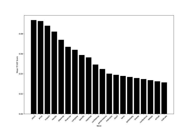
Figure 4: Words with Highest TF-IDF Score for All Explanations

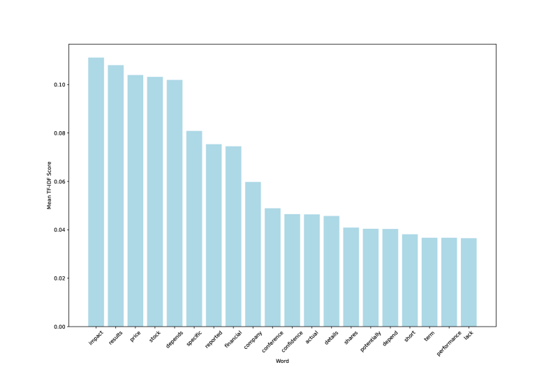
Figure 6: Words with Highest TF-IDF Score for Neutral Explanations

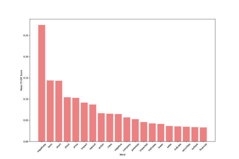
Figure 7: Words with Highest TF-IDF Score for Negative Explanations

Figures 4, 5, 6, and 7 show the words with the highest overall TF-IDF scores by explanation for all explanations, positive, negative, and neutral, respectively. For all explanations, there is no particular pattern with words such as ‘stock,’ ‘price,’ ‘impact,’ ‘results,’ ‘depends,’ ‘financial,’ ‘company,’ ‘specific,’ ‘reported,’ ‘confidence,’ ‘performance,’ ‘indicates,’ ‘short,’ ‘term,’ ‘potentially,’ ‘shares,’ ‘conference,’ ‘details,’ ‘actual,’ and ‘indicate’ appear.

For positive explanations, we start looking at words indicative of positive outcomes and sound financial performance with words such as ‘dictates,’ ‘positive,’ ‘company,’ ‘stock,’ ‘performance,’ ‘price,’ ‘confidence,’ ‘strong,’ ‘increased,’ ‘financial,’ ‘dividend,’ ‘growth,’ ‘likely,’ ‘future,’ ‘investors,’ ‘revenue,’ ‘positively,’ ‘typically,’ ‘boost,’ and ‘potential’ appearing. For neutral explanations, we have only general descriptive indicators, financial metrics, and uncertainty or conditionality with words such as ‘impact,’ ‘results,’ ‘price,’ ‘stock,’ ‘depends,’ ‘specific,’ ‘reported,’ ‘financial,’ ‘company,’ ‘conference,’ ‘confidence,’ ‘actual,’ ‘details,’ ‘shares,’ ‘potentially,’ ‘depend,’ ‘short,’ ‘term,’ ‘performance,’ and ‘lack.’ Finally, for negative explanations, we have words indicating adverse outcomes, financial concerns and legal issues such as ‘negatively,’ ‘term,’ ‘short,’ ‘stock,’ ‘price,’ ‘impact,’ ‘lawsuit,’ ‘action,’ ‘class,’ ‘negative,’ ‘company,’ ‘potential,’ ‘impacted,’ ‘indicates,’ ‘lower,’ ‘sales,’ ‘indicate,’ ‘securities,’ ‘outlook,’ and ‘financial.’ However, this method does not allow distinguishing between correct and incorrect explanations. To do so, we use a supervised approach to characterize the words that best predict if a given answer relates correctly to the outcome.

Having transformed the textual explanations into a structured format, we employ regularized logistic regression models. The choice of logistic regression is motivated by our binary outcome variable: whether the stock price moved in the direction predicted by ChatGPT. By modeling this relationship, we aim to establish the predictive power of the qualitative explanations provided by the model. By training distinct models for positive and negative news explanations, we aim to capture the subtle variations in how optimistic and pessimistic rationale influenced stock price dynamics. This approach provides a more comprehensive view of the market’s sentiment-driven behavior.

In our analysis, understanding the significance and influence of individual features, particularly words in this context, is paramount. To achieve this, we first extract the terms with the highest and lowest coefficients in the logistic regression models. This method provides positive and negative coefficients, allowing us to identify words that had the most pronounced impact on whether the explanations were correct. Each set of words is categorized into “correct” and “incorrect” based on their effect on the predictive accuracy. These words could shed light on the lexicon that ChatGPT relied on and illustrate how certain terms were more aligned with specific ideas.

While individual words are interesting, it is difficult to understand the full impact without their context. To delve deeper into the contextual environment of these influential words, we identify the words that frequently accompany a given target word. We filter out less significant words by setting a threshold percentile for the average TF-IDF, ensuring that the accompanying words list was both relevant and impactful. Through this approach, we are not just looking at words in isolation but also understanding their significance in the broader context, shedding light on the intricate web of relationships that underpin stock market predictions.

6.2 Interpretability Results

Table 11 reports the exercise results for ChatGPT-4’s positive recommendations with several themes. First, the model predicts satisfactorily when its reasoning is related to stock purchases by insiders. Second, the model forecasts accurately when its explanations relate to earnings guidance. Third, the model performs well for themes related to earnings per share or market share. Finally, the model also does well when the theme relates to dividends. On the contrary, the model does worse when its reasoning refers to partnerships or new developments. It also fails when justifying the recommendation with profits, sales, and profitability. One potential reason for the negative influence of profits, sales, and profitability could be that ChatGPT was fed with only the news headlines but not the market expectation regarding firms’ profits or sales at the time of news release. For scheduled events like earnings releases, it is crucial to use the market expectation as the benchmark to tease out the component that moves the market.

Table 12 reports the exercise results for ChatGPT-4’s negative recommendations with several themes. First, the model predicts well when its reasoning is related to risk of downgrade or risk related to credit. Second, the model also predicts satisfactorily when the theme is related to factors that impacted earnings or revenue negatively. Third, the model forecasts accurately when the theme is related to fraud or reputational damages. Finally, the model also does well when its explanations relate to the sale of securities by directors. On the contrary, the model does worse when its reasoning relates to prospects or outlook. It also fails when reasoning about profits, sales, and profitability.

7 Conclusion

In this study, we investigate the potential of ChatGPT and other large language models in predicting stock market returns using sentiment analysis of news headlines. We document several findings that are new to the literature. First, ChatGPT’s assessment scores of news headlines can predict subsequent daily stock returns. Its predictability outperforms traditional sentiment analysis methods from a leading data vendor. Second, more basic LLMs such as GPT-1, GPT-2, and BERT cannot accurately forecast returns while strategies based on ChatGPT-4 deliver the highest Sharpe ratio, indicating return predictability is an emerging capacity of complex language models. Third, the predictability of ChatGPT scores presents in both small and large stocks, suggesting market underreaction to company news. Fourth, predictability is stronger among smaller stocks and stocks with bad news, consistent with limits-to-arbitrage also playing an important role. Finally, we propose a new method to evaluate and understand the models’ reasoning capabilities. By demonstrating the value of LLMs in financial economics, we contribute to the growing body of literature on the applications of artificial intelligence and natural language processing in this domain.

Our research has several implications for future studies. First, it highlights the importance of continued exploration and development of LLMs tailored explicitly for the financial industry. As AI-driven finance evolves, more sophisticated models can be designed to improve the accuracy and efficiency of financial decision-making processes.

Second, our findings suggest that future research could focus more on understanding the mechanisms through which LLMs derive their predictive power. By identifying the factors contributing to models like ChatGPT’s success in predicting stock market returns, researchers can develop more targeted strategies for improving these models and maximizing their utility in finance.

Additionally, as LLMs become more prevalent in the financial industry, it is essential to investigate their potential impact on market dynamics, including price formation, information dissemination, and market stability. Future research can explore the role of LLMs in shaping market behavior and their potential positive and negative consequences for the financial system.

Lastly, future studies could explore the integration of LLMs with other machine learning techniques and quantitative models to create hybrid systems that combine the strengths of different approaches. By leveraging the complementary capabilities of various methods, researchers can further enhance the predictive power of AI-driven models in financial economics.

In short, our study demonstrates the value of ChatGPT in predicting stock market returns. It paves the way for future research on the applications and implications of LLMs in the financial industry. As the field of AI-driven finance continues to expand, the insights gleaned from this research can help guide the development of more accurate, efficient, and responsible models that enhance the performance of financial decision-making processes.

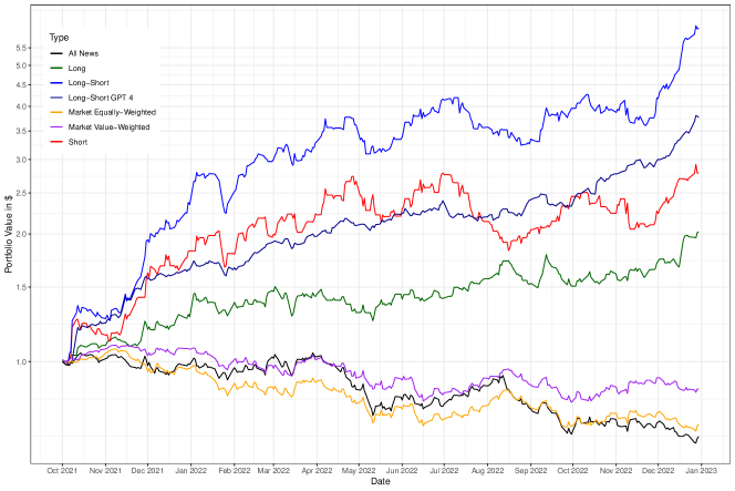
Figure 1: Cumulative Returns of Investing $1 (Without Transaction Costs)

This figure presents the results of different trading strategies without considering transaction costs. If a piece of news is released before 6 a.m. on a trading day, we enter the position at the market opening and exit at the close of the same day. If the news is released after 6 a.m. but before the market close, we enter the position at the market close price of the same day and exit at the close of the next trading day. If the news is announced after the market closes, we assume we enter the position at the next opening price and exit at the close of the next trading day. All the strategies are rebalanced daily. The “All-news” black line corresponds to an equal-weight portfolio in all companies with news the day before (regardless of news direction). The green line corresponds to an equal-weighted portfolio that buys companies with good news, according to ChatGPT 3.5. The red line corresponds to an equal-weighted portfolio that short-sells companies with bad news, according to ChatGPT 3.5. The light blue line corresponds to an equal-weighted zero-cost portfolio that buys companies with good news and short-sells companies with bad news, according to ChatGPT 3.5. The dark blue line corresponds to an equal-weighted zero-cost portfolio that buys companies with good news and short-sells companies with bad news, according to ChatGPT 4. The yellow line corresponds to an equally weighted market portfolio. The purple line corresponds to a value-weighted market portfolio.

This figure presents the results of different trading strategies for different transaction costs. If a piece of news is released before 6 a.m. on a trading day, we enter the position at the market opening and exit at the close of the same day. If the news is released after 6 a.m. but before the market close, we enter the position at the market close price of the same day and exit at the close of the next trading day. If the news is announced after the market closes, we assume we enter the position at the next opening price and exit at the close of the next trading day. All the strategies are rebalanced daily. The black line corresponds to an equal-weighted zero-cost portfolio that buys companies with good news and short-sells companies with bad news, according to ChatGPT 3.5, with zero transaction costs. The dark green line corresponds to the same equal-weighted zero-cost portfolio with a cost of 5 bps per transaction (i.e., 10 bps round trip). The light blue line corresponds to the same equal-weighted zero-cost portfolio with a cost of 10 bps per transaction. The dark blue line corresponds to the same equal-weighted zero-cost portfolio with a cost of 25 bps per transaction. The red line corresponds to an equally weighted market portfolio without transaction costs.

This figure presents the results of different trading strategies for different transaction costs. If a piece of news is released before 6 a.m. on a trading day, we enter the position at the market opening and exit at the close of the same day. If the news is released after 6 a.m. but before the market close, we enter the position at the market close price of the same day and exit at the close of the next trading day. If the news is announced after the market closes, we assume we enter the position at the next opening price and exit at the close of the next trading day. All the strategies are rebalanced daily. The black line corresponds to an equal-weighted short portfolio that buys companies with good news and short-sells companies with bad news, according to ChatGPT 3.5, with zero transaction costs. The dark green line corresponds to the same equal-weighted short portfolio with a cost of 5 basis points per transaction. The light blue line corresponds to the same equal-weighted short portfolio with a cost of 10 basis points per transaction. The dark blue line corresponds to the same equal-weighted short portfolio with a cost of 25 basis points per transaction. The red line corresponds to an equally weighted market portfolio without transaction costs.

The figure shows the words with the highest term-frequency inverse-document-frequency (TF-IDF) scores when considering the universe of explanations of ChatGPT-4 recommendations.

Figure 5: Words with Highest TF-IDF Score for Positive Explanations

The figure shows the words with the highest term-frequency inverse-document-frequency (TF-IDF) scores when considering the universe of explanations of ChatGPT-4 positive recommendations.

The figure shows the words with the highest term-frequency inverse-document-frequency (TF-IDF) scores when considering the universe of explanations of ChatGPT-4 neutral recommendations.

The figure shows the words with the highest term-frequency inverse-document-frequency (TF-IDF) scores when considering the universe of explanations of ChatGPT-4 negative recommendations.

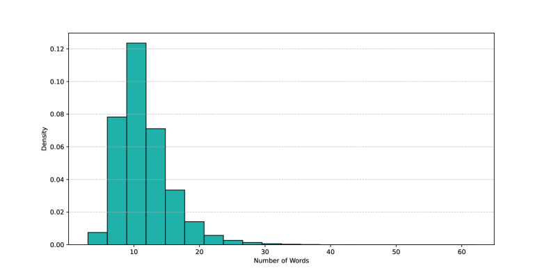
Figure 8: Length Distribution for All Headlines

The figure shows the distribution of length in characters of all news.

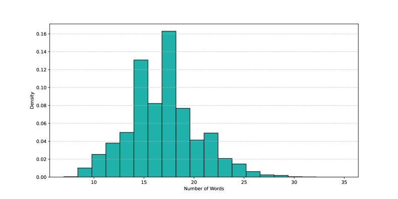
Figure 9: Length Distribution for All Explanations

The figure shows the distribution of length in characters of all news.

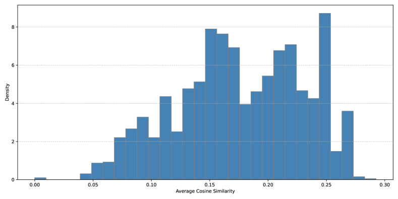
Figure 10: Distribution of Average Explanation Similarity

The figure shows the distribution of the average similarity of explanations. The average similarity is computed using the cosine similarity measure and then taking the row average.

Table 1: Descriptive Statistics

Panel A of this table reports selected descriptive statistics of the daily stock returns in percentage points, the headline length, the response length, the GPT score (1 if ChatGPT says YES, 0 if UNKNOWN, and -1 if NO), and the event sentiment score provided by the data vendor. Panel B reports the correlation between daily stock returns in percentage points, the headline length, the response length, the GPT score, and the event sentiment score.

Panel A. Summary Statistics Mean SD min P25 Median P75 Max N Daily Return (%) $-0$ $5.26$ $-64.97$ $-2.04$ $-0.02$ $1.89$ $237.11$ 60755 Headline Length $76.36$ $28.65$ $21$ $56$ $70$ $90$ $395$ 60755 ChatGPT Response Length $153.31$ $38.04$ $0$ $124$ $151$ $179$ $303$ 60755 GPT Score $0.24$ $0.47$ $-1$ $0$ $0$ $1$ $1$ 60755 Event Sentiment Score $0.18$ $0.49$ $-1$ $0$ $0$ $0$ $1$ 60755

Panel B. Correlations Daily Return (%) Headline Length GPT Resp. Length GPT Score Event Sent. Score Daily Return (%) 1 Headline Length $-0.002$ 1 ChatGPT Response Length $-0.001$ $0.261$ 1 GPT Score $0.018$ $0.081$ $0.441$ 1 Event Sentiment Score $0.005$ $-0.071$ $0.091$ $0.279$ 1

Table 2: Descriptive Statistics of Various Portfolios

This table reports the following statistics of the different trading strategies as specified in Figure 1: Sharpe ratio, mean daily returns, standard deviation of daily returns, and maximum drawdown. The strategies include (i) the long and short legs of the strategy based on ChatGPT 3.5, (ii) the long-short strategy based on ChatGPT 3.5, (iii) the long-short strategy based on ChatGPT 4, (iv) equal-weight and value-weight market portfolios, and (v) an equal-weight portfolio in all stocks with news the day before (regardless of news direction).

	Long (L)	Short (S)	L-S ChatGPT	L-S GPT-4	Market EW	Market VW	All News EW
Sharpe Ratio	1.72	1.86	3.09	3.80	-0.99	-0.39	-0.98
Daily Mean (%)	0.25	0.38	0.63	0.44	-0.10	-0.04	-0.11
Daily Std. Dev. (%)	2.32	3.26	3.25	1.84	1.55	1.49	1.83
Max Drawdown (%)	-16.94	-34.39	-22.79	-10.40	-36.12	-26.68	-38.70

Table 3: Regression of Next Day Returns on Prediction Scores from More Advanced LLMs

This table reports the results of running regressions of the form $r_{i,t+1}=a_{i}+b_{t}+\gamma^{\prime}x_{i,t}+\varepsilon_{i,t+1}$. Where $r_{i,t+1}$ is the next day’s return in percentage points, $a_{i}$ and $b_{t}$ are firm and time fixed effects, respectively. $x_{i,t}$ corresponds to the vector containing prediction scores from different models. The main regressors include scores from three advanced LLMs: (i) ChatGPT 3.5, (ii) ChatGPT 4, and (iii) BART Large. We include the event sentiment score from the data vendor for comparison purposes. We provide an overview of the different LLMs in Appendix A of the paper. The corresponding t-statistics are in parentheses. Standard errors are double clustered by date and firm. All models include firm and time fixed effects. The sample consists of all U.S. common stocks with at least one news headline covering the firm.

(1) (2) (3) (4) (5) (6) GPT-3.5-score $0.259$*** $0.243$*** ($5.259$) ($4.980$) event-sentiment-score $0.058$ $0.038$ $0.118$* ($1.122$) ($0.683$) ($2.272$) GPT-4-score $0.176$*** $0.167$*** ($5.382$) ($4.768$) bart-large-score $0.142$*** ($4.653$) Num.Obs. $60\,755$ $60\,755$ $60\,755$ $60\,755$ $60\,755$ $60\,176$ R2 $0.184$ $0.184$ $0.184$ $0.184$ $0.184$ $0.185$ R2 Adj. $0.121$ $0.121$ $0.121$ $0.121$ $0.121$ $0.121$ R2 Within $0.001$ $0.001$ $0.001$ $0.001$ $0.000$ $0.000$ R2 Within Adj. $0.001$ $0.001$ $0.001$ $0.001$ $0.000$ $0.000$ AIC $370\,534.7$ $370\,534.9$ $370\,534.8$ $370\,536.1$ $370\,560.5$ $367\,175.7$ BIC $409\,811.3$ $409\,820.5$ $409\,811.4$ $409\,821.7$ $409\,837.2$ $406\,374.6$ RMSE $4.75$ $4.75$ $4.75$ $4.75$ $4.75$ $4.76$ Std.Errors by: date & permno by: date & permno by: date & permno by: date & permno by: date & permno by: date & permno FE: date X X X X X X FE: permno X X X X X X + p $<$ 0.1, * p $<$ 0.05, ** p $<$ 0.01, *** p $<$ 0.001

Table 4: Regression of Next Day Returns on Prediction Scores from More Basic LLMs

This table reports the results of running regressions of the form $r_{i,t+1}=a_{i}+b_{t}+\gamma^{\prime}x_{i,t}+\varepsilon_{i,t+1}$. Where $r_{i,t+1}$ is the next day’s return in percentage points, $a_{i}$ and $b_{t}$ are firm and time fixed effects, respectively. $x_{i,t}$ corresponds to the vector containing prediction scores from different models. The main regressors include scores from six more basic LLMs: (i) DistilBart-MNLI-12-1, (ii) GPT-2 Large, (iii) GPT-2, (iv) GPT-1, (v) BERT, and (vi) BERT Large. We provide an overview of the different LLMs in Appendix A of the paper. The corresponding t-statistics are in parentheses. Standard errors are double clustered by date and firm. All models include firm and time fixed effects. The sample consists of all U.S. common stocks with at least one news headline covering the firm.

(1) (2) (3) (4) (5) (6) distilbart-mnli-12-1-score $0.150$*** ($4.919$) GPT-2-large-score $0.035$ ($1.051$) GPT-2-score $0.001$ ($0.025$) GPT-1-score $0.034$ ($1.304$) bert-score $-0.226$ ($-3.703$) bert-large-score $0.001$ ($0.020$) Num.Obs. $60\,755$ $60\,176$ $60\,176$ $60\,755$ $60\,176$ $60\,176$ R2 $0.184$ $0.185$ $0.185$ $0.184$ $0.185$ $0.185$ R2 Adj. $0.121$ $0.121$ $0.121$ $0.121$ $0.121$ $0.121$ R2 Within $0.000$ $0.000$ $0.000$ $0.000$ $0.000$ $0.000$ R2 Within Adj. $0.000$ $0.000$ $0.000$ $0.000$ $0.000$ $0.000$ AIC $370\,547.3$ $367\,194.8$ $367\,195.9$ $370\,566.9$ $367\,180.1$ $367\,195.9$ BIC $409\,823.9$ $406\,393.7$ $406\,394.8$ $409\,843.5$ $406\,379.0$ $406\,394.8$ RMSE $4.75$ $4.76$ $4.76$ $4.75$ $4.76$ $4.76$ Std.Errors by: date & permno by: date & permno by: date & permno by: date & permno by: date & permno by: date & permno FE: date X X X X X X FE: permno X X X X X X + p $<$ 0.1, * p $<$ 0.05, ** p $<$ 0.01, *** p $<$ 0.001

Table 5: Regression of Next Day Returns on Prediction Scores from More Advanced LLMs (Small Stocks)

This table reports the results of running regressions of the form $r_{i,t+1}=a_{i}+b_{t}+\gamma^{\prime}x_{i,t}+\varepsilon_{i,t+1}$. Where $r_{i,t+1}$ is the next day’s return in percentage points, $a_{i}$ and $b_{t}$ are firm and time fixed effects, respectively. $x_{i,t}$ corresponds to the vector containing prediction scores from different models. The main regressors include scores from three advanced LLMs: (i) ChatGPT 3.5, (ii) ChatGPT 4, and (iii) BART Large. We include the event sentiment score from the data vendor for comparison purposes. The corresponding t-statistics are in parentheses. Standard errors are double clustered by date and firm. All models include firm and time fixed effects. The sample used in this analysis consists of Small stocks, defined as those whose market capitalization is below the 10th percentile NYSE market capitalization distribution.

(1) (2) (3) (4) (5) (6) GPT-3.5-score $0.653$*** $0.542$*** ($5.145$) ($4.028$) event-sentiment-score $0.277$* $0.256$+ $0.435$*** ($2.117$) ($1.876$) ($3.567$) GPT-4-score $0.501$*** $0.419$*** ($4.830$) ($3.645$) bart-large-score $0.165$ ($1.504$) Num.Obs. $14\,343$ $14\,343$ $14\,343$ $14\,343$ $14\,343$ $14\,238$ R2 $0.201$ $0.201$ $0.201$ $0.201$ $0.200$ $0.201$ R2 Adj. $0.086$ $0.086$ $0.086$ $0.086$ $0.085$ $0.086$ R2 Within $0.002$ $0.002$ $0.002$ $0.002$ $0.001$ $0.000$ R2 Within Adj. $0.002$ $0.002$ $0.002$ $0.002$ $0.001$ $0.000$ AIC $98\,043.0$ $98\,039.8$ $98\,041.0$ $98\,038.7$ $98\,052.1$ $97\,320.5$ BIC $111\,731.4$ $111\,735.8$ $111\,729.4$ $111\,734.7$ $111\,740.5$ $110\,957.8$ RMSE $6.51$ $6.51$ $6.51$ $6.51$ $6.51$ $6.50$ Std.Errors by: date & permno by: date & permno by: date & permno by: date & permno by: date & permno by: date & permno FE: date X X X X X X FE: permno X X X X X X + p $<$ 0.1, * p $<$ 0.05, ** p $<$ 0.01, *** p $<$ 0.001

Table 6: Regression of Next Day Returns on Prediction Scores from More Basic LLMs (Small Stocks)

This table reports the results of running regressions of the form $r_{i,t+1}=a_{i}+b_{t}+\gamma^{\prime}x_{i,t}+\varepsilon_{i,t+1}$. Where $r_{i,t+1}$ is the next day’s return in percentage points, $a_{i}$ and $b_{t}$ are firm and time fixed effects, respectively. $x_{i,t}$ corresponds to the vector containing prediction scores from different models. The main regressors include scores from six more basic LLMs: (i) DistilBart-MNLI-12-1, (ii) GPT-2 Large, (iii) GPT-2, (iv) GPT-1, (v) BERT, and (vi) BERT Large. The corresponding t-statistics are in parentheses. Standard errors are double clustered by date and firm. All models include firm and time fixed effects. The sample used in this analysis consists of Small stocks, defined as those whose market capitalization is below the 10th percentile NYSE market capitalization distribution.

(1) (2) (3) (4) (5) (6) distilbart-mnli-12-1-score $0.207$+ ($1.895$) GPT-2-large-score $0.019$ ($0.216$) GPT-2-score $0.064$ ($0.765$) GPT-1-score $0.008$ ($0.098$) bert-score $-0.492$** ($-2.598$) bert-large-score $0.018$ ($0.096$) Num.Obs. $14\,343$ $14\,238$ $14\,238$ $14\,343$ $14\,238$ $14\,238$ R2 $0.200$ $0.201$ $0.201$ $0.200$ $0.202$ $0.201$ R2 Adj. $0.084$ $0.085$ $0.085$ $0.084$ $0.086$ $0.085$ R2 Within $0.000$ $0.000$ $0.000$ $0.000$ $0.001$ $0.000$ R2 Within Adj. $0.000$ $0.000$ $0.000$ $0.000$ $0.001$ $0.000$ AIC $98\,063.3$ $97\,322.6$ $97\,322.0$ $98\,066.4$ $97\,314.2$ $97\,322.6$ BIC $111\,751.7$ $110\,959.9$ $110\,959.3$ $111\,754.8$ $110\,951.5$ $110\,959.9$ RMSE $6.51$ $6.50$ $6.50$ $6.51$ $6.50$ $6.50$ Std.Errors by: date & permno by: date & permno by: date & permno by: date & permno by: date & permno by: date & permno FE: date X X X X X X FE: permno X X X X X X + p $<$ 0.1, * p $<$ 0.05, ** p $<$ 0.01, *** p $<$ 0.001

Table 7: Regression of Next Day Returns on Prediction Scores from More Advanced LLMs (Non-Small Stocks)

This table reports the results of running regressions of the form $r_{i,t+1}=a_{i}+b_{t}+\gamma^{\prime}x_{i,t}+\varepsilon_{i,t+1}$. Where $r_{i,t+1}$ is the next day’s return in percentage points, $a_{i}$ and $b_{t}$ are firm and time fixed effects, respectively. $x_{i,t}$ corresponds to the vector containing prediction scores from different models. The main regressors include scores from three advanced LLMs: (i) ChatGPT 3.5, (ii) ChatGPT 4, and (iii) BART Large. We include the event sentiment score from the data vendor for comparison purposes. The corresponding t-statistics are in parentheses. Standard errors are double clustered by date and firm. All models include firm and time fixed effects. The sample consists of non-small stocks, defined as those whose market cap is above the 10th percentile NYSE market capitalization distribution.

(1) (2) (3) (4) (5) (6) GPT-3.5-score $0.148$** $0.158$** ($3.084$) ($3.280$) event-sentiment-score $-0.041$ $-0.060$ $-0.005$ ($-0.830$) ($-1.163$) ($-0.112$) GPT-4-score $0.097$** $0.111$*** ($3.252$) ($3.491$) bart-large-score $0.144$*** ($4.695$) Num.Obs. $46\,402$ $46\,402$ $46\,402$ $46\,402$ $46\,402$ $45\,928$ R2 $0.218$ $0.218$ $0.218$ $0.218$ $0.218$ $0.219$ R2 Adj. $0.159$ $0.159$ $0.159$ $0.159$ $0.158$ $0.159$ R2 Within $0.000$ $0.000$ $0.000$ $0.000$ $0.000$ $0.001$ R2 Within Adj. $0.000$ $0.000$ $0.000$ $0.000$ $0.000$ $0.001$ AIC $265\,328.7$ $265\,329.8$ $265\,329.2$ $265\,329.3$ $265\,341.2$ $262\,823.9$ BIC $294\,082.6$ $294\,092.4$ $294\,083.1$ $294\,091.9$ $294\,095.1$ $291\,517.9$ RMSE $3.93$ $3.93$ $3.93$ $3.93$ $3.93$ $3.94$ Std.Errors by: date & permno by: date & permno by: date & permno by: date & permno by: date & permno by: date & permno FE: date X X X X X X FE: permno X X X X X X + p $<$ 0.1, * p $<$ 0.05, ** p $<$ 0.01, *** p $<$ 0.001

Table 8: Regression of Next Day Returns on Prediction Scores from More Basic LLMs (Non-Small Stocks)

This table reports the results of running regressions of the form $r_{i,t+1}=a_{i}+b_{t}+\gamma^{\prime}x_{i,t}+\varepsilon_{i,t+1}$. Where $r_{i,t+1}$ is the next day’s return in percentage points, $a_{i}$ and $b_{t}$ are firm and time fixed effects, respectively. $x_{i,t}$ corresponds to the vector containing prediction scores from different models. The main regressors include scores from six more basic LLMs: (i) DistilBart-MNLI-12-1, (ii) GPT-2 Large, (iii) GPT-2, (iv) GPT-1, (v) BERT, and (vi) BERT Large. The corresponding t-statistics are in parentheses. Standard errors are double clustered by date and firm. All models include firm and time fixed effects. The sample consists of non-small stocks, defined as those whose market cap is above the 10th percentile NYSE market capitalization distribution.

(1) (2) (3) (4) (5) (6) distilbart-mnli-12-1-score $0.146$*** ($4.894$) GPT-2-large-score $0.030$ ($0.947$) GPT-2-score $-0.014$ ($-0.539$) GPT-1-score $0.056$* ($2.332$) bert-score $-0.165$** ($-2.795$) bert-large-score $-0.011$ ($-0.200$) Num.Obs. $46\,402$ $45\,928$ $45\,928$ $46\,402$ $45\,928$ $45\,928$ R2 $0.218$ $0.219$ $0.219$ $0.218$ $0.219$ $0.219$ R2 Adj. $0.159$ $0.158$ $0.158$ $0.158$ $0.159$ $0.158$ R2 Within $0.001$ $0.000$ $0.000$ $0.000$ $0.000$ $0.000$ R2 Within Adj. $0.001$ $0.000$ $0.000$ $0.000$ $0.000$ $0.000$ AIC $265\,316.8$ $262\,848.3$ $262\,848.9$ $265\,336.7$ $262\,839.8$ $262\,849.1$ BIC $294\,070.7$ $291\,542.3$ $291\,542.8$ $294\,090.6$ $291\,533.7$ $291\,543.1$ RMSE $3.93$ $3.94$ $3.94$ $3.93$ $3.94$ $3.94$ Std.Errors by: date & permno by: date & permno by: date & permno by: date & permno by: date & permno by: date & permno FE: date X X X X X X FE: permno X X X X X X + p $<$ 0.1, * p $<$ 0.05, ** p $<$ 0.01, *** p $<$ 0.001

Table 9: Average Next Day’s Return by Prediction Score

This table reports several statistics for the portfolios implied by different models. Columns Neg, Pos, and LS shows the daily average returns in percentage points (0.1 corresponds to 0.1%) for the long, neutral, short, and long-short portfolio. Column t LS shows the t-statistic of the daily returns for the long-short portfolio. $\alpha_{M}$ shows the daily alpha with respect to the CAPM model, t $\alpha_{M}$ is the t-statistic, and $R2_{M}$ is the R-sq. from the CAPM model in percentage points. $\alpha_{FF5}$, t $\alpha_{FF5}$, and $R^{2}_{FF5}$ show the same but with respect to the 5-factor model of [18]. We provide an overview of the different LLMs in Appendix A of the paper. Panel A reports results for all U.S. common stocks with at least one news headline covering the firm, Panel B analyzes the sample of small stocks (below the 10th percentile NYSE market capitalization), and Panel C analyzes the remaining non-small stocks.

Panel A. Full Sample: All Stocks

Model	Pos	Neut	Neg	LS	t LS	$\alpha_{M}$	t $\alpha_{M}$	$R2_{M}$	$\alpha_{FF5}$	t $\alpha_{FF5}$	$R^{2}_{FF5}$
Gpt-4	0.09	-0.18	-0.35	0.44	4.24	0.45	4.31	1.14	0.41	4.01	5.20
Gpt-3.5	0.25	-0.21	-0.38	0.63	3.44	0.63	3.41	0.47	0.60	3.28	4.15
Gpt-1	-0.10	0.01	-0.19	0.09	0.69	0.09	0.71	0.24	0.09	0.67	0.41
Gpt-2	-0.03	-0.20	0.20	-0.23	-1.38	-0.23	-1.37	0.03	-0.24	-1.39	1.83
Gpt-2-Large	-0.06	-0.02	-0.16	0.10	0.92	0.10	0.95	0.40	0.10	0.94	0.64
Bart-Large	-0.01	0.08	-0.16	0.15	1.40	0.15	1.41	0.04	0.13	1.25	1.91
Distilbart-Mnli-12-1	-0.04	0.12	-0.28	0.24	2.12	0.24	2.13	0.08	0.22	1.91	3.77
Bert	-0.23	-0	-0.08	-0.14	-1.16	-0.12	-1.05	12.60	-0.09	-0.79	17.99
Bert-Large	-0.06	-0.06	-0.11	0.04	0.23	0.05	0.25	0.36	0.04	0.19	4.24
Event-Sentiment	-0.04	-0.11	-0.32	0.29	1.94	0.28	1.90	0.47	0.25	1.70	3.04

Panel B. Small Stocks

Model	Pos	Neut	Neg	LS	t LS	$\alpha_{M}$	t $\alpha_{M}$	$R2_{M}$	$\alpha_{FF5}$	t $\alpha_{FF5}$	$R^{2}_{FF5}$
Gpt-4	0.02	-0.82	-0.88	0.90	3.13	0.90	3.12	0.88	0.88	3.07	3.88
Gpt-3.5	0.07	-0.51	-0.97	1.04	2.72	1.03	2.72	2.84	1.05	2.78	5.60
Gpt-1	-0.40	-0.31	-0.51	0.10	0.35	0.10	0.34	0.10	0.13	0.41	0.70
Gpt-2	-0.24	-0.81	-0.14	-0.10	-0.36	-0.10	-0.36	0	-0.11	-0.42	1.20
Gpt-2-Large	-0.23	-0.30	-0.39	0.16	0.55	0.16	0.55	0	0.20	0.68	0.65
Bart-Large	-0.19	-1.98	-0.48	0.29	1.09	0.29	1.10	0.02	0.28	1.06	1.04
Distilbart-Mnli-12-1	-0.25	-2.69	-0.46	0.20	0.73	0.20	0.73	0.11	0.21	0.74	1.26
Bert	-0.88	0.06	-0.08	-0.81	-4.09	-0.81	-4.27	6.57	-0.80	-4.17	8.32
Bert-Large	-0.15	-0.22	-0.54	0.40	1.30	0.39	1.29	1.17	0.42	1.38	3.58
Event-Sentiment	-0.26	-0.23	-0.79	0.53	2	0.53	2	0.12	0.57	2.11	0.64

Panel C. Non-Small Stocks

Model	Pos	Neut	Neg	LS	t LS	$\alpha_{M}$	t $\alpha_{M}$	$R2_{M}$	$\alpha_{FF5}$	t $\alpha_{FF5}$	$R^{2}_{FF5}$
Gpt-4	0.12	0.10	-0.20	0.32	3.32	0.33	3.37	0.71	0.29	2.99	4.07
Gpt-3.5	0.29	-0.06	-0.13	0.42	2.51	0.41	2.46	1.18	0.36	2.19	4.57
Gpt-1	0.02	0.06	-0.01	0.03	0.36	0.03	0.39	0.31	0.04	0.48	0.50
Gpt-2	0.06	-0	0.14	-0.08	-1.12	-0.07	-1.07	0.98	-0.07	-1.07	2.31
Gpt-2-Large	-0.02	0.10	-0.02	0	0.05	0.01	0.08	0.41	0.01	0.09	0.85
Bart-Large	0.10	0.32	-0.12	0.21	2.13	0.22	2.16	0.33	0.20	2.01	1.88
Distilbart-Mnli-12-1	0.09	0.40	-0.24	0.33	3.13	0.33	3.18	0.70	0.31	2.93	3.89
Bert	-0	0.01	-0.02	0.01	0.10	0.04	0.37	18.39	0.07	0.74	24.87
Bert-Large	0.02	0.12	0.18	-0.17	-1.06	-0.16	-1.01	1.02	-0.16	-1.03	6.41
Event-Sentiment	0.03	-0.03	0.04	-0.01	-0.05	-0.02	-0.10	1.01	-0.05	-0.33	3.83

Table 10: Sharpe Ratio and Number of Stocks in Each Leg by Model

This table reports the annualized Sharpe ratio of the long-short portfolio implied by different models. The table also reports the 25th percentile, mean, median, and 75th percentile of the number of stocks in the long ($N_{+}$) and in the short ($N_{-}$) legs. The models include ChatGPT 3.5, ChatGPT 4, Distilbart, Ravenpack, Bart-Large, Gpt-2-Large, Gpt-1, Bert-Large, Bert, Gpt-2. We provide an overview of the different LLMs in Appendix A of the paper. Panel A reports results for all U.S. common stocks with at least one news headline covering the firm, Panel B analyzes the sample of small stocks (below the 10th percentile NYSE market capitalization), and Panel C analyzes the remaining non-small stocks.

Panel A. Full Sample: All Stocks

Model	Sharpe	$N_{+}$25th	$N_{+}$mean	$N_{+}$median	$N_{+}$75th	$N_{-}$25th	$N_{-}$mean	$N_{-}$median	$N_{-}$75th
Gpt-4	3.8	59	98.52	107	140	13	23.30	23	33
Gpt-3.5	3.09	28	50.86	51	72	1	3.84	4	6
Distilbart-Mnli-12-1	1.9	104	167.87	160	234	11	22.06	21	32
Event-Sentiment	1.74	21	44.44	48	61	2	8.82	5	9
Bart-Large	1.26	21.50	148.04	150	210.50	4	23.71	24	34.25
Gpt-2-Large	0.82	8	59.84	61	83.50	2	12.37	12.50	18
Gpt-1	0.62	89	138.23	136	187	14	26.03	25	36
Bert-Large	0.2	21.25	156.32	162.50	223.50	0	2.77	2	4
Bert	$<$0	7.75	36.17	43	53.25	0	0.27	0	0
Gpt-2	$<$0	15.75	99.55	104.50	144	3	24.25	25	35

Panel B. Small Stocks

Model	Sharpe	$N_{+}$25th	$N_{+}$mean	$N_{+}$median	$N_{+}$75th	$N_{-}$25th	$N_{-}$mean	$N_{-}$median	$N_{-}$75th
Gpt-4	2.98	19	25.52	26	32	2	4.24	4	6
Gpt-3.5	2.59	10	14.07	14	18	0	0.72	0	1
Event-Sentiment	1.91	8	12.63	13	16	0	3.63	1	3
Bert-Large	1.24	28	43.74	39	54	0	0.52	0	1
Bart-Large	1.04	26.25	44.65	37	56.75	2	4.31	4	6
Distilbart-Mnli-12-1	0.69	29	47.52	38	59	2	3.92	4	5
Gpt-2-Large	0.53	9	16.89	15	22	1	3.60	3	5
Gpt-1	0.33	23	37.32	32	48	4	7.24	6	9
Gpt-2	$<$0	16	28.53	25	36.75	4	6.92	6	9
Bert	$<$0	7	9.35	10	12.75	0	0.02	0	0

Panel C. Non-Small Stocks

Model	Sharpe	$N_{+}$25th	$N_{+}$mean	$N_{+}$median	$N_{+}$75th	$N_{-}$25th	$N_{-}$mean	$N_{-}$median	$N_{-}$75th
Gpt-4	2.99	49	76.40	80	108	9	19.66	19	28.50
Distilbart-Mnli-12-1	2.82	76	126.60	120	173	8.50	18.70	17	27
Gpt-3.5	2.26	20.50	38.63	37	54	1	3.22	3	5
Bart-Large	1.92	31	111.47	106.50	157	4.25	20.17	19	28
Gpt-1	0.33	64	105.85	106	142	10	19.74	19	27.50
Bert	0.09	8.25	28.34	33	41	0	0.26	0	0
Gpt-2-Large	0.04	12.50	45.99	47.50	64	2	9.40	9	14
Event-Sentiment	$<$0	15	33.46	32	44	1.50	5.65	4	7
Bert-Large	$<$0	36	120.49	124	171.25	0	2.34	2	4
Gpt-2	$<$0	19.50	76	77	107.75	6.25	18.58	18	28

Table 11: ChatGPT-4 Positive Recommendations Interpretability

This table reports on Panel A the most relevant words for making good predictions and their context. The coefficient is the slope from a regularized logistic regression model. The frequencies are normalized to the 0-1 range via TF-IDF, so the magnitude of the coefficient can be interpreted as feature importance. Larger coefficients are more relevant for accurate predictions.

Panel A: Positive Influence
Influential Word	Coefficient	Top Accompanying Words
purchase	0.61	future, shows, significant, number, demonstrates
guidance	0.50	indicate, revenue, stability, earnings, likely
share	0.39	earnings, market, indicate, typically, lead
dividends	0.37	generally, seen, sign, generating, profits
higher	0.35	lead, typically, attracts, indicate, sales
returns	0.31	shareholder, stability, attract, indicate, value
generating	0.28	profits, sign, generally, seen, sharing
number	0.26	significant, future, acquisition, shows, purchase
sharing	0.26	generating, profits, sign, generally, seen
insider	0.23	future, positively, significant, number, indicate
Panel B: Negative Influence
Influential Word	Coefficient	Top Accompanying Words
development	-0.54	progress, positively, new, investor, lead
profits	-0.45	generating, sign, generally, seen, sharing
stability	-0.28	sign, generally, seen, indicating, commitment
profitability	-0.27	announcement, shareholder, typically, quarterly…
sales	-0.24	indicate, likely, higher, boost, positively
commitment	-0.21	sign, generally, seen, shareholder, stability
declaring	-0.20	sign, seen, generally, quarterly, indicating
demand	-0.19	lead, increase, partnership, positively, likely
partnership	-0.18	likely, lead, revenue, boost, increase
lead	-0.16	revenue, typically, partnership, higher, collab…

Table 12: ChatGPT-4 Negative Recommendations Interpretability

This table reports on Panel A the most relevant words for making good predictions and their context. The coefficient is the slope from a regularized logistic regression model. The frequencies are normalized to the 0-1 range via TF-IDF, so the magnitude of the coefficient can be interpreted as feature importance. Larger coefficients are more relevant for accurate predictions.

Influential Word	Coefficient	Top Accompanying Words
significant	0.92	indicate, lack, selling, number, chairman
indicate	0.78	lack, significant, selling, number, future
risk	0.64	downgrade, credit, investor, higher, outlook
headline	0.48	suggests, likely, earnings, issues, sales
impacted	0.46	likely, earnings, revenue, reduced, drop
director	0.45	indicate, lack, number, sale, future
issues	0.43	headline, sales, impacting, revenue, reduced
number	0.39	lack, indicate, significant, selling, future
fraud	0.36	securities, reputational, investor, loss, headline
reputational	0.33	securities, fraud, losses, headline, lead
Influential Word	Coefficient	Top Accompanying Words
prospects	-0.90	lack, significant
credit	-0.63	downgrade, outlook, future, risk, investor
chairman	-0.62	indicate, lack, selling, significant, number
lack	-0.52	indicate, selling, number, significant, future
outlook	-0.47	downgrade, future, credit, investor, lowered
sale	-0.47	lack, indicate, number, future, director
revenue	-0.44	lower, likely, decreased, expectations, profit
earnings	-0.40	likely, impacted, lower, sales, decline
losses	-0.38	reputational, decreased, securities, impacts, lead
sales	-0.32	lower, decreased, indicate, decline, earnings

Appendix A: Model Summaries

In this section, we present an overview of the ten different models that we study in this paper. We order them by their release date.

Model 1. GPT-1: Estimated Number of Parameters: 117 million, Release Date: Feb 2018, Website: https://huggingface.co/docs/transformers/model_doc/openai-gpt.

Generative Pre-trained Transformer 1 (GPT-1) was the first of OpenAI’s large language models following Google’s invention of the transformer architecture in 2017. It was introduced in February 2018 by OpenAI. GPT-1 had 117 million parameters and significantly improved previous state-of-the-art language models. One of its strengths was its ability to generate fluent and coherent language when given a prompt or context. It was based on the transformer architecture and trained on a large corpus of books.

Model 2. BERT: Estimated Number of Parameters: 110 million, Release Date: Nov 2, 2018, Website: https://huggingface.co/bert-base-uncased.

BERT (Bidirectional Encoder Representations from Transformers) is a family of language models introduced in 2018 by researchers at Google. It is based on the transformer architecture and was initially implemented in English at two model sizes: BERT BASE and BERT Large. Both models were pre-trained on the Toronto BookCorpus and English Wikipedia. BERT was pre-trained simultaneously on language modeling and next-sentence prediction. As a result of this training process, BERT learns latent representations of words and sentences in context. It can be fine-tuned with fewer resources on smaller datasets to optimize its performance on specific tasks such as NLP tasks and sequence-to-sequence-based language generation tasks.

Model 3. BERT-Large: Estimated Number of Parameters: 336 million, Release Date: Nov 2, 2018, Website: https://huggingface.co/bert-large-uncased.

BERT (Bidirectional Encoder Representations from Transformers) is a family of language models introduced in 2018 by researchers at Google. It is based on the transformer architecture and was initially implemented in English at two model sizes: BERT BASE and BERT Large. Both models were pre-trained on the Toronto BookCorpus and English Wikipedia. BERT was pre-trained simultaneously on language modeling and next-sentence prediction. As a result of this training process, BERT learns latent representations of words and sentences in context. It can be fine-tuned with fewer resources on smaller datasets to optimize its performance on specific tasks such as NLP tasks and sequence-to-sequence-based language generation tasks.

Model 4. GPT-2: Estimated Number of Parameters: 124 million, Release Date: Feb 14, 2019, Website: https://huggingface.co/gpt2.

Generative Pre-trained Transformer 2 (GPT-2) is a large language model by OpenAI, the second in their foundational series of GPT models1. It was pre-trained on BookCorpus, a dataset of over 7,000 unpublished fiction books from various genres, and trained on a dataset of 8 million web pages1. GPT-2 was partially released in February 2019. It is a decoder-only transformer model of deep neural networks, which uses attention in place of previous recurrence- and convolution-based architectures. The model demonstrated strong zero-shot and few-shot learning on many tasks. This is the smallest version of GPT-2, with 124M parameters.

Model 5. GPT-2-Large: Estimated Number of Parameters: 774 million, Release Date: Feb 1, 2019, Website: https://huggingface.co/gpt2-large.

GPT-2 Large is the 774M parameter version of GPT-2. Generative Pre-trained Transformer 2 (GPT-2) is a large language model by OpenAI, the second in their foundational series of GPT models1. It was pre-trained on BookCorpus, a dataset of over 7,000 unpublished fiction books from various genres, and trained on a dataset of 8 million web pages1. GPT-2 was partially released in February 2019. It is a decoder-only transformer model of deep neural networks, which uses attention in place of previous recurrence- and convolution-based architectures. The model demonstrated strong zero-shot and few-shot learning on many tasks.

Model 6. BART-Large: Estimated Number of Parameters: 400 million, Release Date: Oct 29, 2019, Website: https://huggingface.co/facebook/bart-large-mnli.

BART (large-sized model) is a pre-trained model on the English language, introduced in the paper “BART: Denoising Sequence-to-Sequence Pre-training for Natural Language Generation, Translation, and Comprehension” by Lewis et al. (2019). It uses a standard seq2seq/machine translation architecture with a bidirectional encoder (like BERT) and a left-to-right decoder (similar to GPT). The pre-training task involves randomly shuffling the order of the original sentences and a novel in-filling scheme, where text spans are replaced with a single mask token. BART is particularly effective when fine-tuned for text generation but also works well for comprehension tasks. It matches the performance of RoBERTa with comparable training resources on GLUE and SQuAD. It achieves new state-of-the-art results on a range of abstractive dialogue, question-answering, and summarization tasks, with gains of up to 6 ROUGE. BART (large-sized model) has nearly 400M parameters.

Model 7. Distilbart-Mnli-12-1: Estimated Number of Parameters: $<$ 400 million , Release Date: Sep 21, 2020, Website: https://huggingface.co/valhalla/distilbart-mnli-12-1.

Distilbart-Mnli-12-1 is a distilled version of bart-large-mnli created using the No Teacher Distillation technique proposed for BART summarisation by Huggingface. It was released on September 21, 2020. It copies alternating layers from bart-large-mnli and is fine-tuned more on the same data. The performance drop is very little compared to the original model.

Model 8. GPT-3.5: Estimated Number of Parameters: 175 billion, Release Date: Nov 30, 2022, Website: https://platform.openai.com/docs/models.

GPT-3.5 is a fined-tuned version of the GPT3 (Generative Pre-Trained Transformer) model. It has 175 billion parameters and is trained on a dataset of text and code up to June 2021. GPT-3.5 models can understand and generate natural language or code. The most capable and cost-effective model in the GPT-3.5 family is gpt-3.5-turbo, which has been optimized for chat using the Chat completions API but works well for traditional completions tasks. GPT-3.5 effectively performs various tasks, including text generation, translation, summarization, question answering, code generation, and creative writing.

Model 9. GPT-4: Estimated Number of Parameters: 1.76 trillion, Release Date: Mar 14, 2023, Website: https://platform.openai.com/docs/models

GPT-4 is a multimodal large language model created by OpenAI and the fourth in its series of GPT foundation models. OpenAI released it on March 14, 2023. As a transformer-based model, GPT-4 uses a paradigm where pre-training using both public data and ”data licensed from third-party providers” is used to predict the next token. After this step, the model was fine-tuned with reinforcement learning feedback from humans and AI for human alignment and policy compliance. OpenAI did not release the technical details of GPT-4; the technical report explicitly refrained from specifying the model size, architecture, or hardware used during either training or inference. GPT-4 has several capabilities, including generating text that is indistinguishable from human-written text; translating languages with high accuracy; writing different kinds of creative content, such as poems, code, scripts, musical pieces, emails, and letters; and answering questions in an informative way, even if they are open-ended, challenging, or strange.

Model 10. Event-Sentiment Estimated Number of Parameters: NA, Release Date: NA, Website: https://www.ravenpack.com/

RavenPack Event Sentiment Score

Appendix B: Prompts for Other LLMs

This appendix provides details on the prompts for other LLMs. While a key focus of our paper is on ChatGPT, we compare the results of ChatGPT with those of more basic models such as BERT, GPT-1, and GPT-2. We employ a different strategy because those models cannot follow instructions or answer specific questions.

GPT-1 and GPT-2 are autocomplete models. Hence, we use the following sentence that the models complete:

News: + headline + f”Will this increase or decrease the stock price of firm? This will make firm’s stock price go ”

The usual response is “up,” “down,” followed by a brief sentence fragment. The answers are usually not fully legible but include positive and negative words. We count the positive words against the negative words and assign a $+1$ for every positive and a $-1$ for every negative. We then consider the sentiment positive if the sum is positive and vice versa. The positive words are ‘up,’ ‘high,’ ‘sky,’ ‘top,’ ‘increase,’ ‘stratosphere,’ ‘boom,’ ‘roof,’ ‘skyrocket,’ ‘soar,’ ‘surge,’ ‘climb,’ ‘rise,’ ‘rising,’ ‘expand,’ ‘flourish.’ The negative words are ‘down,’ ‘low,’ ‘bottom,’ ‘decrease,’ ‘back,’ ‘under,’ ‘plummet,’ ‘drop,’ ‘decline,’ ‘tumble,’ ‘fall,’ ‘contract,’ ‘struggle.’

BERT is only able to complete one word out of a sentence. Hence, we ask it to complete the following sentence:

Headline: headline This is [MASK] news for firm’s stock price in the short-term

Where [MASK] is the corresponding word that BERT will input. The answers set consists of ‘good,’ ‘the,’ ‘big,’ and ‘bad.’ We classify ‘good’ as +1, ’bad’ as -1, and the others as zero.

The BART model is capable of zero-shot classification. This means it can classify text according to predefined categories without seeing examples of what corresponds to a good category. We provide each headline and then classify it into one of the following categories:

1. good news for the stock price of firm in the short term

2. bad news for the stock price of firm in the short term

3. not news for the stock price of firm in the short term

We then assign a numerical score of +1 for good, -1 for bad, and 0 for not.

References

- [1] Daron Acemoglu, David Autor, Jonathon Hazell and Pascual Restrepo “Artificial Intelligence and Jobs: Evidence from Online Vacancies” In Journal of Labor Economics 40.S1 University of Chicago Press, 2022, pp. S293–S340 DOI: 10.1086/718327/SUPPL–“˙˝FILE/20462DATA.ZIP
- [2] Daron Acemoglu and Pascual Restrepo “Tasks, Automation, and the Rise in U.S. Wage Inequality” In Econometrica 90.5 John Wiley & Sons, Ltd, 2022, pp. 1973–2016 DOI: 10.3982/ECTA19815
- [3] Ajay Agrawal, Joshua S. Gans and Avi Goldfarb “Artificial Intelligence: The Ambiguous Labor Market Impact of Automating Prediction” In Journal of Economic Perspectives 33.2 American Economic Association, 2019, pp. 31–50 DOI: 10.1257/JEP.33.2.31
- [4] Tania Babina, Anastassia Fedyk, Alex Xi He and James Hodson “Artificial Intelligence, Firm Growth, and Product Innovation” In SSRN Electronic Journal Elsevier BV, 2022 DOI: 10.2139/SSRN.3651052
- [5] Scott R. Baker, Nicholas Bloom and Steven J. Davis “Measuring economic policy uncertainty” In Quarterly Journal of Economics 131.4 Oxford Academic, 2016, pp. 1593–1636 DOI: 10.1093/qje/qjw024
- [6] Victor L Bernard and Jacob K Thomas “Post-earnings-announcement drift: delayed price response or risk premium?” In Journal of Accounting research 27 JSTOR, 1989, pp. 1–36
- [7] Jules H Binsbergen, Xiao Han and Alejandro Lopez-Lira “Man versus Machine Learning: The Term Structure of Earnings Expectations and Conditional Biases” In The Review of Financial Studies 36.6 Oxford Academic, 2023, pp. 2361–2396 DOI: 10.1093/RFS/HHAC085
- [8] Jules H. Binsbergen et al. “Man vs. Machine Learning: The Term Structure of Earnings Expectations and Conditional Biases” Working Pa.27843, Working Paper Series, 2020, pp. undefined–undefined DOI: 10.3386/w27843
- [9] Leland Bybee, Bryan T. Kelly, Asaf Manela and Dacheng Xiu “The Structure of Economic News” In Working Paper Elsevier BV, 2019 DOI: 10.2139/ssrn.3446225
- [10] Leland Bybee, Bryan T. Kelly, Asaf Manela and Dacheng Xiu “Business News and Business Cycles” In SSRN Electronic Journal Elsevier BV, 2021 DOI: 10.2139/SSRN.3446225
- [11] Charles W. Calomiris and Harry Mamaysky “How news and its context drive risk and returns around the world” In Journal of Financial Economics 133.2 North-Holland, 2019, pp. 299–336 DOI: 10.1016/J.JFINECO.2018.11.009
- [12] John L. Campbell et al. “The information content of mandatory risk factor disclosures in corporate filings” In Review of accounting studies 19.1 Boston: Springer US, 2014, pp. 396–455 DOI: 10.1007/S11142-013-9258-3/TABLES/11
- [13] Louis KC Chan, Narasimhan Jegadeesh and Josef Lakonishok “Momentum strategies” In The journal of Finance 51.5 Wiley Online Library, 1996, pp. 1681–1713
- [14] Andrew Chin and Yuyu Fan “Leveraging Text Mining to Extract Insights from Earnings Call Transcripts” In Journal Of Investment Management 21.1, 2023 URL: https://joim.com/leveraging-text-mining-to-extract-insights-from-earnings-call-transcripts/
- [15] Lauren Cohen, Christopher Malloy and Quoc Nguyen “Lazy Prices” In Journal of Finance 75.3 Blackwell Publishing Ltd, 2020, pp. 1371–1415 DOI: 10.1111/jofi.12885
- [16] Tyler Cowen and Alexander T. Tabarrok “How to Learn and Teach Economics with Large Language Models, Including GPT” In SSRN Electronic Journal, 2023 DOI: 10.2139/SSRN.4391863
- [17] Stefano DellaVigna and Joshua M Pollet “Investor inattention and Friday earnings announcements” In The journal of finance 64.2 Wiley Online Library, 2009, pp. 709–749
- [18] Eugene F. Fama and Kenneth R. French “A five-factor asset pricing model” In Journal of Financial Economics 116.1 North-Holland, 2015, pp. 1–22 DOI: http://dx.doi.org/10.1016/j.jfineco.2014.10.010
- [19] Anastassia Fedyk and James Hodson “When can the market identify old news?” In Journal of Financial Economics 149.1 North-Holland, 2023, pp. 92–113 DOI: 10.1016/J.JFINECO.2023.04.008
- [20] Joachim Freyberger, Andreas Neuhierl and Michael Weber “Dissecting Characteristics Nonparametrically” In The Review of Financial Studies 33.5, 2020, pp. 2326–2377 DOI: 10.1093/rfs/hhz123
- [21] Diego Garcia “Sentiment during Recessions” In The Journal of Finance 68.3 John Wiley & Sons, Ltd, 2013, pp. 1267–1300 DOI: 10.1111/JOFI.12027
- [22] Maclean Peter Gaulin “Risk Fact or Fiction: The Information Content of Risk Factor Disclosures” In Dissertation, 2017
- [23] Shihao Gu, Bryan Kelly and Dacheng Xiu “Empirical Asset Pricing via Machine Learning” In The Review of Financial Studies 33.5, 2020, pp. 2223–2273 DOI: 10.1093/rfs/hhaa009
- [24] Anne Lundgaard Hansen and Sophia Kazinnik “Can ChatGPT Decipher Fedspeak?” In SSRN Electronic Journal, 2023 DOI: 10.2139/SSRN.4399406
- [25] Stephen Hansen, Michael McMahon and Andrea Prat “Transparency and Deliberation Within the FOMC: A Computational Linguistics Approach*” In The Quarterly Journal of Economics 133.2 Oxford Academic, 2018, pp. 801–870 DOI: 10.1093/qje/qjx045
- [26] David Hirshleifer, Sonya Seongyeon Lim and Siew Hong Teoh “Driven to distraction: Extraneous events and underreaction to earnings news” In The journal of finance 64.5 Wiley Online Library, 2009, pp. 2289–2325
- [27] Gerard Hoberg and Gordon Phillips “Text-Based Network Industries and Endogenous Product Differentiation” In Journal of Political Economy 124.5, 2016, pp. 1423–1465 DOI: 10.1086/688176
- [28] Narasimhan Jegadeesh and Di Wu “Word power: A new approach for content analysis” In Journal of Financial Economics 110.3, 2013, pp. 712–729 DOI: https://doi.org/10.1016/j.jfineco.2013.08.018
- [29] Fuwei Jiang, Joshua Lee, Xiumin Martin and Guofu Zhou “Manager sentiment and stock returns” In Journal of Financial Economics 132.1 North-Holland, 2019, pp. 126–149 DOI: 10.1016/j.jfineco.2018.10.001
- [30] Hao Jiang, Sophia Zhengzi Li and Hao Wang “Pervasive underreaction: Evidence from high-frequency data” In Journal of Financial Economics 141.2 North-Holland, 2021, pp. 573–599 DOI: 10.1016/J.JFINECO.2021.04.003
- [31] Wei Jiang, Yuehua Tang, Rachel Jiqiu Xiao and Vincent Yao “Surviving the FinTech disruption”, 2022
- [32] Shikun Ke, José Luis Montiel Olea and James Nesbit “A Robust Machine Learning Algorithm for Text Analysis” In Working Paper, 2019
- [33] Zheng Ke, Bryan T Kelly and Dacheng Xiu “Predicting Returns with Text Data” In University of Chicago, Becker Friedman Institute for Economics Working Paper, 2019 DOI: http://dx.doi.org/10.2139/ssrn.3074808
- [34] Hyungjin Ko and Jaewook Lee “Can Chatgpt Improve Investment Decision? From a Portfolio Management Perspective” In SSRN Electronic Journal Elsevier BV, 2023 DOI: 10.2139/SSRN.4390529
- [35] Anton Korinek “Language Models and Cognitive Automation for Economic Research”, 2023 DOI: 10.3386/W30957
- [36] Alejandro Lopez-Lira “Risk Factors That Matter: Textual Analysis of Risk Disclosures for the Cross-Section of Returns” In SSRN Electronic Journal Elsevier BV, 2019 DOI: 10.2139/ssrn.3313663
- [37] Asaf Manela and Alan Moreira “News implied volatility and disaster concerns” In Journal of Financial Economics 123.1 North-Holland, 2017, pp. 137–162 DOI: 10.1016/j.jfineco.2016.01.032
- [38] Shakked Noy and Whitney Zhang “Experimental Evidence on the Productivity Effects of Generative Artificial Intelligence” In SSRN Electronic Journal Elsevier BV, 2023 DOI: 10.2139/SSRN.4375283
- [39] David E Rapach, Jack K Strauss and Guofu Zhou “International stock return predictability: What is the role of the united states?” In Journal of Finance 68.4 Cutler, Poterba,Summers, 2013, pp. 1633–1662 DOI: 10.1111/jofi.12041
- [40] Paul C. Tetlock “Giving Content to Investor Sentiment: The Role of Media in the Stock Market” In The Journal of Finance 62.3 John Wiley & Sons, Ltd, 2007, pp. 1139–1168 DOI: 10.1111/J.1540-6261.2007.01232.X
- [41] Paul C. Tetlock “All the News That’s Fit to Reprint: Do Investors React to Stale Information?” In The Review of Financial Studies 24.5 Oxford Academic, 2011, pp. 1481–1512 DOI: 10.1093/RFS/HHQ141
- [42] Paul C. Tetlock, Maytal Saar-Tsechansky and Sofus Macskassy “More Than Words: Quantifying Language to Measure Firms’ Fundamentals” In Journal of Finance 63.3 John Wiley & Sons, Ltd, 2008, pp. 1437–1467 DOI: 10.1111/j.1540-6261.2008.01362.x
- [43] Ashish Vaswani et al. “Attention is all you need” In Advances in Neural Information Processing Systems 2017-Decem, 2017, pp. 5999–6009
- [44] Michael Webb “The Impact of Artificial Intelligence on the Labor Market” In SSRN Electronic Journal Elsevier BV, 2019 DOI: 10.2139/SSRN.3482150
- [45] Shijie Wu et al. “BloombergGPT: A Large Language Model for Finance”, 2023
- [46] Qianqian Xie et al. “The Wall Street Neophyte: A Zero-Shot Analysis of ChatGPT Over MultiModal Stock Movement Prediction Challenges”, 2023
- [47] Qianqian Xie et al. “PIXIU: A Large Language Model, Instruction Data and Evaluation Benchmark for Finance” In arXiv preprint arXiv:2306.05443, 2023
- [48] Kai-Cheng Yang and Filippo Menczer “Large language models can rate news outlet credibility”, 2023 URL: https://arxiv.org/abs/2304.00228v1